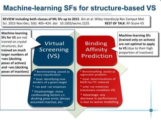
ML scoring functions
to improve structure‐based
binding affinity prediction
and virtual screening
Dr Pedro Ballester, INSERM (France)
Workshop on the Mathematics of Drug Design/Discovery, The Fields Institute 2018 (Toronto, Canada)
twitter.com/pjballester
linkedin.com/in/pedroballester/
pedro.ballester@inserm.fr
Molecular docking applications
Predict whether a
molecule docked to
a given target is a
true binder from the
docked structure
Predict the affinity of
a molecule bound to a
given target from the
crystal structure
Each application rely on the prediction provided by a scoring function (SF)
 important to develop SFs that are optimal for the intended application
Machine-learning
Scoring Functions
(RF-Score, 2010)
1. Generic: structures of proteins from other families may
improve prediction (complement structures of target)
2. This requires an algorithm that builds sufficiently flexible
regression models  Random Forest (Breiman, 2001)
3. Advantage: circumventing a priori assumptions about the
SF’s functional form, which may reduce modelling error
Training and testing RF-Score
pKd/i C.C – C.I N.C – I.I PDB
0.49 1254 – 0 166 – 0 1w8l
– – – – – – – –
13.00 2324 – 0 919 – 0 2ada
pKd/i C.C – C.I N.C – I.I PDB
1.40 858 – 0 0 – 0 2hdq
– – – – – – – –
13.96 4476 – 0 283 – 0 7cpa
Random Forest (RF) training
(descriptor selection, model selection)
RF-Score
(description and training choices)
1105
195
Generation of descriptors (dcutoff, binning, interatomic types)
Training set (1105 complexes) Test set (195 complexes)
1w8l
pKi=0.49
1gu1
pKi=4.52
2ada
pKi=13
2hdq
pKi=1.4
1e66
pKi=9.89
7cpa
pKi=13.96
2010: 1st version  Rp=0.78
Scoring Function Corsortium using RF-Score code
2008
2013
http://infochim.u-strasbg.fr/CS3_2012/Lectures/Sotriffer.pdf
Best features? RF-Score v2 in 2014
 a data-driven feature
selection procedure was
more effective than a
knowledge-based one
Systematic numerical study:
– Interatomic distance cutoffs
– Interatomic distance bin sizes
– Atom hybridisation and protonation
state
– Angle between HBD, HBA and H
atoms.
– Covalent and van der Waals radius
of atoms.
– Basic feature selection.
– Model selection by OOB
Elem(c12,b2)_spr1_oob
• Rp: 0.787  0.803
(= training set, = test set)
The effect of training with more data: MLR vs RF
Classical SFs
)(1 1 klcutoff
K
k
L
lij ddx j i
   
Machine-learning SFs )( mRF xfp 
1. Autodock Vina off-the-shelf
as a baseline (model 1)
2. Retrained Vina using its 6
features and MLR (model 2)
3. Retrained Vina using its 6
features and RF (model 3)
4. RF training on a merged
vector with the 42 RF-Score
v1 + Vina features (model 4)
The effect of training with more data: MLR vs RF
2013
2012
2010
2007
2002
From 5 releases of the
PDBbind database
Generated 4 time-stamped data partitions with
same test set (new structures released in 2013)
2013
Test set
(382
complexes)
2010
2007
2002
2012
model 2 vs model 3: substituting
MLR by RF using Vina features 
MLR does not improve with more
data, but RF does!
model 3 vs model 4: increasing
the number of features also
beneficial with RF
model 2 vs model 4: large gain
over classical SFs due to RF being
able to assimilate larger feature
and data sets
model 4
 released as RF-Score v3
Rp on new complexes (2013 only)
2002
2007
2010
2012
Trade-off quality vs quantity of training data
Exploiting a larger data volume is more
important for the performance of RF-Score than
restricting to a smaller set of higher data quality
Molecules 2015, 20, 10947-10962; doi:10.3390/molecules200610947
TestsetRp
# of training complexes
scoring function Rp Rs SD
RF-Score::Elem-v2 0.803 0.797 1.54
RF-Score::Elem-v1 0.776 0.762 1.58
X-Score::HMScore 0.644 0.705 1.83
DrugScoreCSD
0.569 0.627 1.96
SYBYL::ChemScore0.555 0.585 1.98
DS::PLP1 0.545 0.588 2.00
GOLD::ASP 0.534 0.577 2.02
SYBYL::G-Score 0.492 0.536 2.08
DS::LUDI3 0.487 0.478 2.09
DS::LigScore2 0.464 0.507 2.12
GlideScore-XP 0.457 0.435 2.14
DS::PMF 0.445 0.448 2.14
GOLD::ChemScore 0.441 0.452 2.15
by NHA 0.431 0.517 2.15
SYBYL::D-Score 0.392 0.447 2.19
IMP::RankScore 0.322 0.348 2.25
DS::Jain 0.316 0.346 2.24
GOLD::GoldScore 0.295 0.322 2.29
SYBYL::PMF-Score0.268 0.273 2.29
SYBYL::F-Score 0.216 0.243 2.35
SFs tested on PDBbind benchmark (now CASF2007)
Rp +0.132: Random Forest (RF) with simple intermolecular features
instead of linear regression and expert-selected features  RF-Score-
v1 (Ballester & Mitchell 2010; doi:10.1093/bioinformatics/btq112r)
Rp +0.027: RF with data-selected features  RF-Score-v2
(Ballester, Schreyer & Blundell 2014; doi:10.1021/ci500091r)
ClassicalSFsMachine-learningSFs
Performance of the best classical SF for this
problem  X-Score (Cheng et al. 2009;
doi:10.1021/ci9000053)
Rp +0.023: Deep Neural Networks instead of RF (2017-18)  (*)
(*) Deep Learning applied to this problem
 TNet-BP (Cang & Wei 2017;
doi:10.1371/journal.pcbi.1005690) &
 Spatial MPNN (Feinberg et al. 2018;
arXiv:1803.04465v1)
SFs for Binding affinity prediction: Challenges
• Understanding for which targets generic SFs are better than
target-specific. Which factors determine this?
• Understanding which regression algorithm will work better on a
given target: e.g. Do classical SFs perform better than ML SFs
for targets with few pKd/i–measured co-crystallised ligands?
• To which extent data from other targets help binding affinity
(pKd/i) prediction depending on the considered target and why?
Machine-learning SFs for structure-based VS
Machine-learning
SFs for VS are not
trained on crystal
structures, but
trained on much
larger numbers of
+ves (docking
poses of actives)
and –ves (docking
poses of inactives)
Machine-learning SFs
(trained only on actives)
are not optimal to apply
to VS (due to their high
proportion of inactives)
REVIEW including both classes of ML SFs up to 2015: Ain et al. Wiley Interdiscip Rev Comput Mol
Sci. 2015 Nov-Dec; 5(6): 405–424. doi: 10.1002/wcms.1225 REST OF TALK: RF-Score-VS
DUD-E: Generating data to build RF-Score-VS
• DUD-E: Mysinger et al. 2012 (dx.doi.org/10.1021/jm300687e)
• 102 protein targets: on average 224 actives per target with their
reported activities + 50 decoys per active (<= 1uM)
• Decoys: assumed inactive (~physicochemical to actives, but
dissimilar chemical structure to reduce chance of being active)
• After docking with Smina implementation of Vina, 50 docking
poses x (15 426 actives and 893 897 decoys) across targets
• 50 poses per molecule, but only lowest Vina score for training.
• Three RF-Score features: v1 (2010), v2 (2014) and v3 (2015).
• In the end, 909,323 docked molecules to train & validate each SF
• Processed data at https://wojcikowski.pl/rfscorevs/data/
Cross-validating machine-learning SFs for VS
: i.e. some actives known for the target
: i.e. some actives known for all 102 targets
: i.e. absolutely no actives known for the target
DUD-E: Performance of classical and ML SFs for VS
Averages in 5
folds: EF1%=38.96
ROC AUC=0.84
across all targets
Docking engine
(similar results
with DOCK3.6
& DOCK6.6)
RF-Score v3 did just OK, as it is only trained on PDBbind crystal
structures (not on docked poses of actives and inactives)
Horiz. RF-Score-VS are trained on docked
poses of actives & inactives of each target
 3 to 10 times larger EF than classical SFs
Per-target RF-Score-VS
with a high median EF,
but very large variability
(i.e. poor on a few
targets, great on most)
Wójcikowski M, Ballester PJ & Siedlecki P (2017) Scientific Reports (dx.doi.org/10.1038/srep46710)
DUD-E: scoring in the presence of inactives
• RF-Score-VS: need to exploit inactive data too
– Predicted active: top 1% of all docked molecules ranked by
predicted affinity (directly with Vina, RF-Score-VS v2 from 5CV)
– Red points indicate inactive compounds (false positives) and
green points are actives (true positives) within top 1% of the SF
AutoDock Vina
(16.2% hit rate)
Horizontally-trained
RF-Score-VS v2
(55.6% hit rate)
Wójcikowski M, Ballester PJ & Siedlecki P (2017) Scientific Reports (dx.doi.org/10.1038/srep46710)
Rp=-0.18 Rp=0.56
DEKOIS: validating RF-Score-VS on a 2nd resource
• DEKOIS 2.0: Bauer et al. 2013 (dx.doi.org/10.1021/ci400115b)
• 81 targets: we used 76 targets (4 in DUD-E, 1 w/out crystal struct.)
• filtered out any nearly identical ligand or decoy to any
ligand/decoy present in DUD-E (tanimoto score of at least 0.99;
OpenBabel FP2 fingerprints).
• Each DEKOIS target has 40 ligands and 1200 decoys, our pruning
removed on average 18.6 (46.5%) ligands and 188 (15.7%) decoys.
• retained DEKOIS 2.0 ligands &decoys were docked using Autodock
Vina with default settings, as previously done with DUD-E.
• Re-score with RF-Score-VS trained on entire DUD-E data> this SF
is available at https://github.com/oddt/rfscorevs_binary
• NEXT: reporting performance of RF-Score-VS on DEKOIS data
DEKOIS: validating RF-Score-VS on 2nd resource
Even less favourable that the ‘vertical split’ scenario (RF-Score-VS is applied to a not included
in the training set): here targets, actives & inactives in this test set were not in the training set
RF-Score v3 is trained on PDBbind crystal structures (not
on docked poses of actives and inactives as RF-Score-VS)
Mean
EF1%=9.84
(10.57 DUD-E)
Mean
EF1%=7.81
(10.37 DUD-E)
Mean
EF1%=3.95
(10.98 DUD-E)
Mean
EF1%=2.94
(5.42 DUD-E)
Wójcikowski M, Ballester PJ & Siedlecki P (2017) Scientific Reports (dx.doi.org/10.1038/srep46710)
we could not evaluate RF-Score-VS on 4 targets in
common between DEKOIS and DUD-E because
almost all the actives were the same. This is the
scenario where RF-Score-VS works best (‘horizontal’)
ML SFs for VS: opportunities and challenges
• Training on (semi-)synthetic data (i.e. docking poses with
measured target-activity), EF1% > 20 for 75% of DUD-E targets
• at least 1 co-crystallised ligand + >40 actives. Exciting: a ML SF
could be generated for a large number of targets nowadays.
• However, target knowledge and molecular modelling required,
esp. for 25% of DUD-E targets (EF1% < 20). Some challenges:
1) Assuming that every active binds non-covalently to the
same binding site as the co-crystallised ligand. Which don’t?
2) Docking poses are typically suboptimal because Vina used
with defaults  investigate best settings for the target
3) Actives & inactives only approximates target promiscuity
Summary
• Machine-learning SFs shown to be more accurate than classical
SFs at predicting pKd of diverse protein-ligand complexes
• The performance of RF-Score improves with training set size, but
not that of classical SFs (MLR-based)  gap will broaden
• Regarding structural descriptors, data-driven Feature Selection
(FS) leads to more predictive SFs than knowledge-based FS
• A target-specific RF-Score-VS can be built for any target with at
least one ligand-bound crystal structure and > 40 actives
• Much room for improvement: applying other ML algorithms,
more targets and training data, identifying the best SF for each
target…
Acknowledgements
• Hongjian Li, Kwong-Sak Leung, Man-Hon Wong
(Chinese University of Hong Kong)
• Adrian Schreyer, Tom Blundell (University of
Cambridge)
• John Mitchell (University of Cambridge)
• Maciek Wójcikowski (Institute of Biochemistry and
Biophysics, Polish Academy of Sciences)
• Pawel Siedlecki (University of Warsaw)
Collaborators Funding
RF-Score-v1 performance on diverse test set
Rp=0.78
Rp=0.64
Rp=0.55
Prospective
application of
RF-Score v1 (2012)
• DHQase-2: only three known active scaffolds (1 from HTS)
• Hierarchical VS: USR (3) on 9M cpds > GOLD on 4K USR hits  RF-
Score  test top 148 cpds (N. Howard, Univ of Cambridge)
• Very high hit rates of ~ 25% with Ki  100 M  100 new and
structurally diverse actives (£5,000 cost)
Impact of similarities between training/test proteins
• Test set from PDBbind benchmark (2007 core set with
195 complexes). Each point is the Rp of a SF on this
common test set
• Each SF trained on nested training sets (e.g. 1st
training set with 14 complexes comes from removing
all training complexes with protein sequence
similarity > 0.2 to the protein of at least one test
complex. Larger sets obtained with higher thresholds
• Unlike X-Score, RF-Score improves when the
complexes with the most similar proteins are
included in the training set, but not only from them!
Biomolecules 2018, 8(1), 12; doi:10.3390/biom8010012
Train/test on crystal structures vs docking poses
• Binding affinity prediction is often carried out on the
docked pose of a known binder rather than its co-
crystallised pose.
• Our results suggest than pose generation error is in
general far less damaging for binding affinity
prediction than it is currently believed.
• Another contribution of our study is the proposal of a
procedure that largely corrects for this error.
• The resulting machine-learning scoring function, RF-
Score v4 is freely available at
http://ballester.marseille.inserm.fr/rf-score-4.tgz
BMC Bioinformatics2016,17(Suppl 11):308; doi:10.1186/s12859-016-1169-4
Support Vector Regression (SVR)-Score
https://doi.org/10.1007/978-3-
642-34123-6_2
RF-Score codes for binding affinity prediction
• RF-Score v4 (trained on 3441 complexes with 47 features):
http://ballester.marseille.inserm.fr/rf-score-4.tgz
• RF-Score v3 (trained on 2959 complexes with 42 features):
http://ballester.marseille.inserm.fr/rf-score-3.tgz
• RF-Score v2 (python code to generate v2 descriptors):
https://bitbucket.org/aschreyer/rfscore
• RF-Score v1 (C code to generate v1 descriptors and R scripts):
http://ballester.marseille.inserm.fr/RF-Score-v1.zip

Machine-learning scoring functions for molecular docking

  • 1.
    ML scoring functions toimprove structure‐based binding affinity prediction and virtual screening Dr Pedro Ballester, INSERM (France) Workshop on the Mathematics of Drug Design/Discovery, The Fields Institute 2018 (Toronto, Canada) twitter.com/pjballester linkedin.com/in/pedroballester/ pedro.ballester@inserm.fr
  • 2.
    Molecular docking applications Predictwhether a molecule docked to a given target is a true binder from the docked structure Predict the affinity of a molecule bound to a given target from the crystal structure Each application rely on the prediction provided by a scoring function (SF)  important to develop SFs that are optimal for the intended application
  • 3.
    Machine-learning Scoring Functions (RF-Score, 2010) 1.Generic: structures of proteins from other families may improve prediction (complement structures of target) 2. This requires an algorithm that builds sufficiently flexible regression models  Random Forest (Breiman, 2001) 3. Advantage: circumventing a priori assumptions about the SF’s functional form, which may reduce modelling error
  • 4.
    Training and testingRF-Score pKd/i C.C – C.I N.C – I.I PDB 0.49 1254 – 0 166 – 0 1w8l – – – – – – – – 13.00 2324 – 0 919 – 0 2ada pKd/i C.C – C.I N.C – I.I PDB 1.40 858 – 0 0 – 0 2hdq – – – – – – – – 13.96 4476 – 0 283 – 0 7cpa Random Forest (RF) training (descriptor selection, model selection) RF-Score (description and training choices) 1105 195 Generation of descriptors (dcutoff, binning, interatomic types) Training set (1105 complexes) Test set (195 complexes) 1w8l pKi=0.49 1gu1 pKi=4.52 2ada pKi=13 2hdq pKi=1.4 1e66 pKi=9.89 7cpa pKi=13.96 2010: 1st version  Rp=0.78
  • 5.
    Scoring Function Corsortiumusing RF-Score code 2008 2013 http://infochim.u-strasbg.fr/CS3_2012/Lectures/Sotriffer.pdf
  • 6.
    Best features? RF-Scorev2 in 2014  a data-driven feature selection procedure was more effective than a knowledge-based one Systematic numerical study: – Interatomic distance cutoffs – Interatomic distance bin sizes – Atom hybridisation and protonation state – Angle between HBD, HBA and H atoms. – Covalent and van der Waals radius of atoms. – Basic feature selection. – Model selection by OOB Elem(c12,b2)_spr1_oob • Rp: 0.787  0.803 (= training set, = test set)
  • 7.
    The effect oftraining with more data: MLR vs RF Classical SFs )(1 1 klcutoff K k L lij ddx j i     Machine-learning SFs )( mRF xfp  1. Autodock Vina off-the-shelf as a baseline (model 1) 2. Retrained Vina using its 6 features and MLR (model 2) 3. Retrained Vina using its 6 features and RF (model 3) 4. RF training on a merged vector with the 42 RF-Score v1 + Vina features (model 4)
  • 8.
    The effect oftraining with more data: MLR vs RF 2013 2012 2010 2007 2002 From 5 releases of the PDBbind database Generated 4 time-stamped data partitions with same test set (new structures released in 2013) 2013 Test set (382 complexes) 2010 2007 2002 2012 model 2 vs model 3: substituting MLR by RF using Vina features  MLR does not improve with more data, but RF does! model 3 vs model 4: increasing the number of features also beneficial with RF model 2 vs model 4: large gain over classical SFs due to RF being able to assimilate larger feature and data sets model 4  released as RF-Score v3 Rp on new complexes (2013 only) 2002 2007 2010 2012
  • 9.
    Trade-off quality vsquantity of training data Exploiting a larger data volume is more important for the performance of RF-Score than restricting to a smaller set of higher data quality Molecules 2015, 20, 10947-10962; doi:10.3390/molecules200610947 TestsetRp # of training complexes
  • 10.
    scoring function RpRs SD RF-Score::Elem-v2 0.803 0.797 1.54 RF-Score::Elem-v1 0.776 0.762 1.58 X-Score::HMScore 0.644 0.705 1.83 DrugScoreCSD 0.569 0.627 1.96 SYBYL::ChemScore0.555 0.585 1.98 DS::PLP1 0.545 0.588 2.00 GOLD::ASP 0.534 0.577 2.02 SYBYL::G-Score 0.492 0.536 2.08 DS::LUDI3 0.487 0.478 2.09 DS::LigScore2 0.464 0.507 2.12 GlideScore-XP 0.457 0.435 2.14 DS::PMF 0.445 0.448 2.14 GOLD::ChemScore 0.441 0.452 2.15 by NHA 0.431 0.517 2.15 SYBYL::D-Score 0.392 0.447 2.19 IMP::RankScore 0.322 0.348 2.25 DS::Jain 0.316 0.346 2.24 GOLD::GoldScore 0.295 0.322 2.29 SYBYL::PMF-Score0.268 0.273 2.29 SYBYL::F-Score 0.216 0.243 2.35 SFs tested on PDBbind benchmark (now CASF2007) Rp +0.132: Random Forest (RF) with simple intermolecular features instead of linear regression and expert-selected features  RF-Score- v1 (Ballester & Mitchell 2010; doi:10.1093/bioinformatics/btq112r) Rp +0.027: RF with data-selected features  RF-Score-v2 (Ballester, Schreyer & Blundell 2014; doi:10.1021/ci500091r) ClassicalSFsMachine-learningSFs Performance of the best classical SF for this problem  X-Score (Cheng et al. 2009; doi:10.1021/ci9000053) Rp +0.023: Deep Neural Networks instead of RF (2017-18)  (*) (*) Deep Learning applied to this problem  TNet-BP (Cang & Wei 2017; doi:10.1371/journal.pcbi.1005690) &  Spatial MPNN (Feinberg et al. 2018; arXiv:1803.04465v1)
  • 11.
    SFs for Bindingaffinity prediction: Challenges • Understanding for which targets generic SFs are better than target-specific. Which factors determine this? • Understanding which regression algorithm will work better on a given target: e.g. Do classical SFs perform better than ML SFs for targets with few pKd/i–measured co-crystallised ligands? • To which extent data from other targets help binding affinity (pKd/i) prediction depending on the considered target and why?
  • 12.
    Machine-learning SFs forstructure-based VS Machine-learning SFs for VS are not trained on crystal structures, but trained on much larger numbers of +ves (docking poses of actives) and –ves (docking poses of inactives) Machine-learning SFs (trained only on actives) are not optimal to apply to VS (due to their high proportion of inactives) REVIEW including both classes of ML SFs up to 2015: Ain et al. Wiley Interdiscip Rev Comput Mol Sci. 2015 Nov-Dec; 5(6): 405–424. doi: 10.1002/wcms.1225 REST OF TALK: RF-Score-VS
  • 13.
    DUD-E: Generating datato build RF-Score-VS • DUD-E: Mysinger et al. 2012 (dx.doi.org/10.1021/jm300687e) • 102 protein targets: on average 224 actives per target with their reported activities + 50 decoys per active (<= 1uM) • Decoys: assumed inactive (~physicochemical to actives, but dissimilar chemical structure to reduce chance of being active) • After docking with Smina implementation of Vina, 50 docking poses x (15 426 actives and 893 897 decoys) across targets • 50 poses per molecule, but only lowest Vina score for training. • Three RF-Score features: v1 (2010), v2 (2014) and v3 (2015). • In the end, 909,323 docked molecules to train & validate each SF • Processed data at https://wojcikowski.pl/rfscorevs/data/
  • 14.
    Cross-validating machine-learning SFsfor VS : i.e. some actives known for the target : i.e. some actives known for all 102 targets : i.e. absolutely no actives known for the target
  • 15.
    DUD-E: Performance ofclassical and ML SFs for VS Averages in 5 folds: EF1%=38.96 ROC AUC=0.84 across all targets Docking engine (similar results with DOCK3.6 & DOCK6.6) RF-Score v3 did just OK, as it is only trained on PDBbind crystal structures (not on docked poses of actives and inactives) Horiz. RF-Score-VS are trained on docked poses of actives & inactives of each target  3 to 10 times larger EF than classical SFs Per-target RF-Score-VS with a high median EF, but very large variability (i.e. poor on a few targets, great on most) Wójcikowski M, Ballester PJ & Siedlecki P (2017) Scientific Reports (dx.doi.org/10.1038/srep46710)
  • 16.
    DUD-E: scoring inthe presence of inactives • RF-Score-VS: need to exploit inactive data too – Predicted active: top 1% of all docked molecules ranked by predicted affinity (directly with Vina, RF-Score-VS v2 from 5CV) – Red points indicate inactive compounds (false positives) and green points are actives (true positives) within top 1% of the SF AutoDock Vina (16.2% hit rate) Horizontally-trained RF-Score-VS v2 (55.6% hit rate) Wójcikowski M, Ballester PJ & Siedlecki P (2017) Scientific Reports (dx.doi.org/10.1038/srep46710) Rp=-0.18 Rp=0.56
  • 17.
    DEKOIS: validating RF-Score-VSon a 2nd resource • DEKOIS 2.0: Bauer et al. 2013 (dx.doi.org/10.1021/ci400115b) • 81 targets: we used 76 targets (4 in DUD-E, 1 w/out crystal struct.) • filtered out any nearly identical ligand or decoy to any ligand/decoy present in DUD-E (tanimoto score of at least 0.99; OpenBabel FP2 fingerprints). • Each DEKOIS target has 40 ligands and 1200 decoys, our pruning removed on average 18.6 (46.5%) ligands and 188 (15.7%) decoys. • retained DEKOIS 2.0 ligands &decoys were docked using Autodock Vina with default settings, as previously done with DUD-E. • Re-score with RF-Score-VS trained on entire DUD-E data> this SF is available at https://github.com/oddt/rfscorevs_binary • NEXT: reporting performance of RF-Score-VS on DEKOIS data
  • 18.
    DEKOIS: validating RF-Score-VSon 2nd resource Even less favourable that the ‘vertical split’ scenario (RF-Score-VS is applied to a not included in the training set): here targets, actives & inactives in this test set were not in the training set RF-Score v3 is trained on PDBbind crystal structures (not on docked poses of actives and inactives as RF-Score-VS) Mean EF1%=9.84 (10.57 DUD-E) Mean EF1%=7.81 (10.37 DUD-E) Mean EF1%=3.95 (10.98 DUD-E) Mean EF1%=2.94 (5.42 DUD-E) Wójcikowski M, Ballester PJ & Siedlecki P (2017) Scientific Reports (dx.doi.org/10.1038/srep46710) we could not evaluate RF-Score-VS on 4 targets in common between DEKOIS and DUD-E because almost all the actives were the same. This is the scenario where RF-Score-VS works best (‘horizontal’)
  • 19.
    ML SFs forVS: opportunities and challenges • Training on (semi-)synthetic data (i.e. docking poses with measured target-activity), EF1% > 20 for 75% of DUD-E targets • at least 1 co-crystallised ligand + >40 actives. Exciting: a ML SF could be generated for a large number of targets nowadays. • However, target knowledge and molecular modelling required, esp. for 25% of DUD-E targets (EF1% < 20). Some challenges: 1) Assuming that every active binds non-covalently to the same binding site as the co-crystallised ligand. Which don’t? 2) Docking poses are typically suboptimal because Vina used with defaults  investigate best settings for the target 3) Actives & inactives only approximates target promiscuity
  • 20.
    Summary • Machine-learning SFsshown to be more accurate than classical SFs at predicting pKd of diverse protein-ligand complexes • The performance of RF-Score improves with training set size, but not that of classical SFs (MLR-based)  gap will broaden • Regarding structural descriptors, data-driven Feature Selection (FS) leads to more predictive SFs than knowledge-based FS • A target-specific RF-Score-VS can be built for any target with at least one ligand-bound crystal structure and > 40 actives • Much room for improvement: applying other ML algorithms, more targets and training data, identifying the best SF for each target…
  • 21.
    Acknowledgements • Hongjian Li,Kwong-Sak Leung, Man-Hon Wong (Chinese University of Hong Kong) • Adrian Schreyer, Tom Blundell (University of Cambridge) • John Mitchell (University of Cambridge) • Maciek Wójcikowski (Institute of Biochemistry and Biophysics, Polish Academy of Sciences) • Pawel Siedlecki (University of Warsaw) Collaborators Funding
  • 22.
    RF-Score-v1 performance ondiverse test set Rp=0.78 Rp=0.64 Rp=0.55
  • 23.
    Prospective application of RF-Score v1(2012) • DHQase-2: only three known active scaffolds (1 from HTS) • Hierarchical VS: USR (3) on 9M cpds > GOLD on 4K USR hits  RF- Score  test top 148 cpds (N. Howard, Univ of Cambridge) • Very high hit rates of ~ 25% with Ki  100 M  100 new and structurally diverse actives (£5,000 cost)
  • 24.
    Impact of similaritiesbetween training/test proteins • Test set from PDBbind benchmark (2007 core set with 195 complexes). Each point is the Rp of a SF on this common test set • Each SF trained on nested training sets (e.g. 1st training set with 14 complexes comes from removing all training complexes with protein sequence similarity > 0.2 to the protein of at least one test complex. Larger sets obtained with higher thresholds • Unlike X-Score, RF-Score improves when the complexes with the most similar proteins are included in the training set, but not only from them! Biomolecules 2018, 8(1), 12; doi:10.3390/biom8010012
  • 25.
    Train/test on crystalstructures vs docking poses • Binding affinity prediction is often carried out on the docked pose of a known binder rather than its co- crystallised pose. • Our results suggest than pose generation error is in general far less damaging for binding affinity prediction than it is currently believed. • Another contribution of our study is the proposal of a procedure that largely corrects for this error. • The resulting machine-learning scoring function, RF- Score v4 is freely available at http://ballester.marseille.inserm.fr/rf-score-4.tgz BMC Bioinformatics2016,17(Suppl 11):308; doi:10.1186/s12859-016-1169-4
  • 26.
    Support Vector Regression(SVR)-Score https://doi.org/10.1007/978-3- 642-34123-6_2
  • 27.
    RF-Score codes forbinding affinity prediction • RF-Score v4 (trained on 3441 complexes with 47 features): http://ballester.marseille.inserm.fr/rf-score-4.tgz • RF-Score v3 (trained on 2959 complexes with 42 features): http://ballester.marseille.inserm.fr/rf-score-3.tgz • RF-Score v2 (python code to generate v2 descriptors): https://bitbucket.org/aschreyer/rfscore • RF-Score v1 (C code to generate v1 descriptors and R scripts): http://ballester.marseille.inserm.fr/RF-Score-v1.zip

Editor's Notes