This document discusses interactive software demonstrations available through the Wolfram Demonstrations Project that can be used for food engineering education and applications. It provides examples of over 40 demonstrations developed specifically for food and food engineering topics. The demonstrations cover areas like mass balance, heat transfer, fluid flow, microbial kinetics, and particulate technology. They allow users to visually explore concepts and engineering calculations by interactively adjusting parameters and seeing results update in real-time. The demonstrations can be used as teaching tools or by professionals for routine engineering calculations.

1. Wolfram Demonstrations: Free Interactive Software for Food
Engineering Education and Practice
Mark D. Normand • Uri Lesmes •
Maria G. Corradini • Micha Peleg
Received: 4 March 2010 / Accepted: 9 March 2010 / Published online: 30 March 2010
Ó Springer Science+Business Media, LLC 2010
Abstract The Wolfram Demonstrations Project on the
web offers a freely downloadable interactive program,
‘Mathematica Player’, which can be used to view and
manipulate about six thousands Demonstrations to date.
They have been contributed by professionals and amateurs
from around the world and include many that elucidate
scientific and engineering principles through graphical
displays. Some can also be used to do actual engineering
calculations, and of these, about forty have been developed
specifically for food and food engineering applications.
The Project’s Demonstrations are all esthetically attractive,
give brief written explanations of the displays and provide
short descriptions of the theory behind them. Each also
gives typical or representative examples, which are shown
with their corresponding parameter settings. Once a
Demonstration is downloaded, the user can enter and
modify the display parameters using sliders on the screen
and watch the effect almost instantaneously. This makes
the Demonstrations a powerful teaching and learning tool
and an effective aid to professionals in routine engineering
calculations. In this review, the food-related Demonstra-
tions are briefly described and their potential role in Food
Engineering education and practice is assessed.
Keywords Unit operations Á Mass balance Á
Heat transfer Á Particulates Á Flow Á Microbial growth Á
Microbial inactivation Á Risk assessment Á Kinetics
Introduction
Engineering Calculations with the Internet Aid
As in other engineering and scientific disciplines, many
basic food engineering calculations can be automated.
Perhaps the best example is units-conversion, which many
web sites offer. Programming a unit conversion is simple
because all that is needed is choosing the appropriate factor
and its multiplication by the user’s entered value. No
wonder, therefore, that ‘‘converters’’ of many types can be
found on the Internet. Currency convertors are perhaps the
most widely known, but similar web pages enable the user
to convert engineering parameters from British units to
metric and scientific or vice versa.
The next stage in complexity involves the use of an
algebraic equation for the conversion. Perhaps the simplest
is the conversion of °C to °F or vice versa. With the high
speed of today’s computers and the Internet, elaborate
mathematical operations can also be performed so that
even complicated functions can be calculated and plotted.
Calculators that allow the user to write one or more alge-
braic equations and have the program plot them in 2D and
3D displays are perhaps the best known. Some can be
freely downloaded while others can be used online. An
example of an online calculator can be found by opening
http://www.walterzorn.com/grapher/grapher_e.htm. There
is also free software on the Internet that generates and plots
statistical distribution functions, performs a Fourier trans-
form and more.
M. D. Normand Á U. Lesmes Á M. Peleg (&)
Department of Food Science, Chenoweth Laboratory, University
of Massachusetts, Amherst, MA 01003, USA
e-mail: micha.peleg@foodsci.umass.edu
M. G. Corradini
Instituto de Tecnologı´a, Facultad de Ingenierı´a y Ciencias
Exactas, Universidad Argentina de la Empresa, Cdad. de Buenos
Aires, Argentina
123
Food Eng Rev (2010) 2:157–167
DOI 10.1007/s12393-010-9018-0

2. Interactive Programs
Some of the mathematical and engineering programs that
do conversions or more elaborate mathematical calcula-
tions allow the user to change the function parameters
through sliders on a screen. Zooming on maps provided
with driving instructions is a most familiar example. Web
sites that offer this kind of software add a ‘game-like’
element to their use. Adding the option to change a
parameter or a set of parameters continuously also enables
the user to generate and examine several scenarios or
patterns within a very short time and with hardly any effort.
Animation
Many web sites include display of a system having a
‘movie-like’ feature. The richest and best known in Food
Engineering and Food Technology is the collection of
animated graphical displays and interactive calculation
tools developed and posted on the Internet by Professor
R. Paul Singh of UC Davis which are used in his courses—
See [3, 11, 12] and http://www.rpaulsingh.com/animated%
20figures/animationlist.htm. Professor Singh’s posted web
pages cover almost all the standard processes and unit
operations in food production, processing and preservation.
They explain, in a most vivid and colorful way, how major
types of food processing equipment work and the physical
principles on which unit operations are based. The web
pages have been an immensely effective teaching aid and
learning tool. Software in related scientific and engineering
fields, such as heat transfer, fluid dynamics and distillation,
can also be found on the web. Such software comes at
different levels of sophistication, written for users at dif-
ferent levels of preparation. Certain programs are very
basic making them appropriate as a teaching tool while
others are more suitable for trained professionals and
practitioners in a field.
Commercial Software
Much of the software to do specific engineering calculations
is not free. There exist a large variety of such programs, and
it would be difficult to survey them all. However, very few
of these have been designed specifically for food engineers
or food engineering students. A notable exception is
Professor Singh’s eFoodSolver [12], examples of which
can be viewed at http://www.rpaulsingh.com/problems/
problemsbyname.htm. It offers user-friendly calculators
for almost all unit operations that are pertinent to food
processing. The programs to calculate heat transfer in food
containers and the (microbial) lethality of commercial
thermal preservation processes (e.g., [10]) are another
notable exception. However, most of the sterility calcula-
tion software is based on log-linear inactivation kinetics and
other assumptions whose validity ought to be treated with
caution. A few interactive sites allow the user to retrieve
numerical data on isothermal microbial growth and inacti-
vation from large data bases created from published mate-
rial. These sites, some listed in Table 1, also enable the user
to view isothermal survival and growth curves based on the
retrieved parameters. The displayed curves, however, are
generated with traditional inactivation and growth kinetics
models, whose applicability cannot be always taken for
granted.
Table 1 Free on-line software and teaching aids for food engineering education and practice
Name Brief description and source Web link
Food engineering Lecture notes for Introduction to food engineering,
relevant animations and calculation examples
(Prof. Singh, University of California-Davis, USA).
http://www.rpaulsingh.com/teachingfirstpage.htm
Food engineering
applications
A package of 21 free downloadable Microsoft Excel
applications for food engineers (Prof. Peleg,
University of Massachusetts- Amherst, USA).
http://www.people.umass.edu/aew2000/ExcelLinks.html
Pathogen
modeling
program
A package of models to predict the growth and
inactivation of food-borne bacteria, primarily
pathogens, under various environmental conditions.
(United States Dept. of Agriculture, USA).
http://www.arserrc.gov/mfs/PMP7_Start.htm
Growth predictor Growth models of microorganisms as a function of
environmental factors, such as temperature, pH and
water activity.
http://www.ifr.ac.uk/Safety/GrowthPredictor/
Microfit Extraction of growth parameters from challenge test
data and comparison between data sets
http://www.ifr.ac.uk/microfit/
Seafood spoilage
and safety
predictor
Software to predict shelf-life and growth of bacteria
in fresh and lightly preserved seafood.
http://www.dfu.min.dk/micro/sssp/Home/Home.aspx
158 Food Eng Rev (2010) 2:157–167
123

3. The Wolfram Demonstrations Project
Wolfram Research (Champaign, IL) is the commercial
company, named after its founder Stephen Wolfram that has
developed and is marketing the program MathematicaÒ
. It
has launched and is now hosting the ‘Wolfram Demonstra-
tions Project’ (http://www.demonstrations.wolfram.com/).
The ‘Wolfram Demonstrations Project’ contains a very
large collection of interactive software written and con-
tributed by MathematicaÒ
users around the world. Prior to
posting on the Project’s web site, each contributed Dem-
onstration is reviewed and edited by the company’s experts,
to avoid errors in contents and guarantee smooth crash-free
running. Almost all the ‘Demonstrations’ can be previewed
in an animated form by clicking on the ‘watch web preview’
button on each Demonstration’s web page (shown in green
letters at the top right corner of the display). The Math-
ematica Player program, which runs the Demonstrations,
can be downloaded free of charge by following the
instructions on the screen. Once saved in the user’s com-
puter, it will run any of the nearly 6,000 Demonstrations in
the project to date. Each Demonstration has one or more
sliders or other controls, see Fig. 1, which are used to vary
the particular Demonstration’s parameters manually or
automatically. Once a slider is moved or a setter bar clicked,
the displayed function, image, calculated values or any
other object adjust almost instantaneously on the screen to
reflect the new parameters’ setting. [The same is true for the
emitted sound in the acoustic and musical Demonstrations].
In almost all the Demonstrations, the user can also type in
the parameters’ values in order to perform a specific cal-
culation. In addition, each parameter can also be varied
continuously to produce an animated display of its effect.
The direction and speed of the chosen parameter alteration
are chosen by a set of animation controls adjacent to the
particular parameter’s slider. Where pertinent, generated
3D objects can be rotated with the mouse so that they can be
viewed from different angles. The Demonstrations, whose
number grows almost daily, cover a very large variety of
fields, from mathematics, the physical sciences, biology and
engineering to economics and business or music and the
arts. The Demonstrations are aimed at users at different
levels of preparation. Some explain concepts, mathematical
theorems or physical principles at the most rudimentary
level. Examples are siphon action, the Pythagorean theorem
or the leverage of pulley arrays. Other Demonstrations show
the inner operation of machines, such as an internal com-
bustion engine (linear and radial) with a different number of
cylinders, transform color coordinates, process images or
even show visual illusions. But many Demonstrations
deal with advanced and modern mathematical concepts,
such as fractional derivatives, functions of complex vari-
ables, cellular automata and fractals. Many of the Demon-
strations are presented as strikingly beautiful colorful
displays. The aforementioned list of the Demonstrations
attractive features is by no means exhaustive, and the
interested reader will find many enlightening, esthetically
appealing and even entertaining Demonstrations by simply
performing a random search, another option offered by the
project.
Wolfram Demonstrations for Food Engineering
and Processing
With less than a handful number of exceptions, the Food
Engineering and Processing-related Wolfram Demonstra-
tions to date have been contributed by a mathematical
modeling group at the University of Massachusetts at
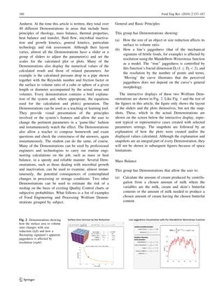
Fig. 1 Calculating heat transfer
through an insulated wall—a
typical display of a Wolfram
Demonstration designed to aid
in Food Engineering
Food Eng Rev (2010) 2:157–167 159
123

4. Amherst. At the time this article is written, they total over
40 different Demonstrations in areas that include basic
principles of rheology, mass balance, thermal properties,
heat balance and transfer, fluid flow, microbial inactiva-
tion and growth kinetics, general kinetics, particulate
technology and risk assessment. Although their layout
varies, almost all the Demonstrations have a slider or a
group of sliders to adjust the parameter(s) and set the
scales for the calculated plot or plots. Many of the
Demonstrations also display the numerical values of the
calculated result and those of related parameters. An
example is the calculated pressure drop in a pipe shown
together with the Reynolds number and friction factor or
the surface to volume ratio of a cube or sphere of a given
length or diameter accompanied by the actual areas and
volumes. Every demonstration contains a brief explana-
tion of the system and, where appropriate, the equations
used for the calculation and plot(s) generation. The
Demonstrations can be used as a teaching or learning tool.
They provide visual presentation of the principles
involved or the system’s features and allow the user to
change the pertinent parameters in a ‘game-like’ fashion
and instantaneously watch the effect. The Demonstrations
also allow a teacher to compose homework and exam
questions and check the correctness of the answers, again
instantaneously. The student can do the same, of course.
Many of the Demonstrations can be used by professional
engineers and technologists to carry out routine engi-
neering calculations on the job, such as mass or heat
balance, in a speedy and reliable manner. Several Dem-
onstrations, such as those dealing with microbial growth
and inactivation, can be used to examine, almost instan-
taneously, the potential consequences of contemplated
changes in processing or storage conditions. Two other
Demonstrations can be used to estimate the risk of a
mishap on the basis of existing Quality Control charts or
subjective probabilities. What follows is a list of examples
of Food Engineering and Processing Wolfram Demon-
strations grouped by subject.
General and Basic Principles
This group has Demonstrations showing:
(a) How the size of an object or size reduction affects its
surface to volume ratio.
(b) How a line’s jaggedness (that of the mechanical
signature of brittle foods, for example) is affected by
resolution using the Mandelbrot–Weierstrass function
as a model. The ‘‘true’’ jaggedness is controlled by
this function’s fractal dimension Df (1 B Df 2), and
the resolution by the number of points and terms.
‘Moving’ the curve illustrates that the perceived
jaggedness does not depend on the curve’s general
morphology.
The interactive displays of these two Wolfram Dem-
onstrations are shown in Fig. 2. Like Fig. 1 and the rest of
the figures in this article, the figure only shows the layout
of the sliders and the plots themselves, but not the snap-
shots. These, which in the actual Demonstrations are
shown on the screen below the interactive display, repre-
sent typical or representative cases created with selected
parameters settings. The snapshots are followed by an
explanation of how the plots were created and/or the
displayed values calculated. Although the explanation and
snapshots are an integral part of every Demonstration, they
will not be shown in subsequent figures because of space
limitations.
Mass Balance
This group has Demonstrations that allow the user to:
(a) Calculate the amount of cream produced by centrifu-
gation from a chosen amount of milk where the
variables are the milk, cream and skim’s butterfat
contents or the amount of milk needed to produce a
chosen amount of cream having the chosen butterfat
content.
Fig. 2 Demonstrations showing
how the surface area to volume
ratio changes with size
reduction (left) and how a
fluctuating signature’s apparent
jaggedness is affected by
resolution (right)
160 Food Eng Rev (2010) 2:157–167
123

5. (b) Calculate the amount of concentrate and vapor
produced in a single-stage evaporator, given the feed
and concentrate’s total solids weight fraction. Or,
alternatively, calculate the amount of feed needed to
produce a chosen amount of concentrate having a
given solids concentration.
(c) Calculate the needed amounts of ‘rich’ and ‘lean’
ingredients in order to make a binary mixture of given
composition, or alternatively, the amount of binary
mixture produced for a chosen amount of the ‘lean’ or
‘rich’ components. The sliders’ layout and settings
and corresponding results are shown in Fig. 3 (top).
All the calculations are based on the assumption that
there is no accumulation in the mixer and that losses
are insignificant.
Heat Balance and Transfer
This group has Demonstrations that allow the user to:
(a) Calculate the logarithmic mean temperature differ-
ence of ideal heat exchangers with the streams’ entry
and exit temperatures as well as their flow directions
(parallel vs. countercurrent) chosen by the user.
(b) Calculate the heat transfer in Wm-2
through an ideal
heat exchanger wall of chosen wall thickness and
thermal conductivity, surface heat transfer coeffi-
cients in the two streams and the logarithmic mean
temperature difference between them.
(c) Calculate the amount of heat in Wm-2
transferred
through an insulated wall as a function of the wall and
insulation’s thickness and conductivity, the surface
heat transfer coefficients at the two sides of the wall
and the temperature difference between them, all
chosen and set by the user—See Fig. 1.
(d) Estimate the net amount of heat to be removed from
1 kg of a food during ideal freezing as a function of
its initial and final temperatures, heat capacities
below and above freezing, freezing point and latent
heat, all chosen and set by the user. Or alternatively,
estimate the amount of heat needed to thaw 1 kg of
food with these chosen parameters. The assumptions
are that the freezing/thawing occurs at a constant
temperature, the thermal properties are not signifi-
cantly affected by temperature in the pertinent range
and that heat losses during the process are negligi-
ble—See Fig. 3 (bottom).
(e) Calculate the heat in Wm-2
or in kWm-2
radiated
from a hot body having a chosen temperature (in °C
or °K) and emissivity to an environment of a chosen
temperature according to the Stefan–Boltzmann
law—See Fig. 4.
(f) Estimate a food’s thermal conductivity below and
above freezing (J kg-1
°C-1
) and latent heat
(kJ kg-1
) from its moisture contents. The displayed
table gives realistic estimates to foods that are
primarily composed from water, carbohydrates and
Fig. 3 Calculating mass balance in mixing two food components
(top) and heat balance in freezing and thawing of foods (bottom) Fig. 4 Calculating heat radiation using the Stefan-Boltzmann law
Food Eng Rev (2010) 2:157–167 161
123

6. protein. This demonstration should not be used for
foods containing a large amount of fat or salt.
(g) Calculate the coefficient of performance (COP) of an
ideal refrigeration cycle using the refrigerant’s
Pressure-Enthalpy diagram. The refrigerant’s enthal-
pies at each of the cycle’s critical points are entered
and can be altered by the user.
Kinetics of Microbial Inactivation
There is growing evidence that microbial survival during
lethal heat treatments (and the application of non-thermal
preservation methods) only rarely follow first-order kinet-
ics as has been traditionally assumed and that there is no
reason that it should (e.g., [5, 13]. Most microbial survival
curves, including those of bacterial spores, follow the
Weibullian or ‘‘power-law’’ model of which log-linear
inactivation is just a special case where the power is equal
to one. Notable exceptions are the survival curves of
Bacilli spores, which frequently exhibit an ‘activation
shoulder’, see: http://www.demonstrations.wolfram.com/
SurvivalCurvesOfBacilliSporesWithAnActivationShoulder/,
and the rare sigmoid survival curves, which might indicate
a mixed population [5].
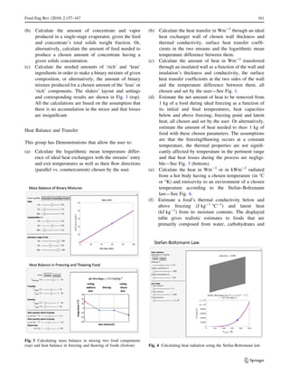
A group of Demonstrations allows the user to create a
temperature profile that emulates the time–temperature
relationship recorded at the coldest point in a food during
its industrial thermal processing in a retort or its prepara-
tion by cooking, baking, roasting or grilling (Fig 5—top).
Once the temperature profile has been chosen, the process’s
settings can be transferred to the inactivation calculation
Demonstrations to generate the corresponding survival
curve (Fig. 5—bottom) using the Weibullian-log-logistic
(WeLL) model [5]. They can also be used to calculate the
‘equivalent time at a reference temperature’ curve, as
shown in Fig. 6. In order to create plots of the kind shown
in Figs. 5 (bottom) and 6, the user has to enter the targeted
organism or spore’s three survival parameters directly or
with their sliders. They are n, assumed to be constant,
which accounts for the curvature of the isothermal semi-
logarithmic survival curves, Tc, a temperature that marks
the lethal regime’s onset and k the slope of the Weibullian
‘rate parameter’, b(T), at temperatures well above Tc. [The
temperature dependence of b(T) can be created with
another demonstration, not shown]. The WeLL model is a
replacement of the traditional log-linear model, which had
produced the ‘z value’, and the Arrhenius equation based
on a temperature-independent ‘energy of activation’,
whose applicability to microbial survival is highly ques-
tionable on theoretical grounds as well as practical con-
siderations [4, 5]. To calculate and plot the process’s
equivalent time curve (Fig. 6), the user sets the reference
Fig. 5 Simulating the temperature profile during thermal processing
of foods (top) and calculating the corresponding dynamic microbial
inactivation curve using the Weibull-log-logistic (WeLL) equation as
the targeted organism’s survival model (bottom)
Fig. 6 Calculating the equivalent time at a reference temperature
curve during thermal processing of foods using the Weibull-log-
logistic (WeLL) equation as the targeted organism’s survival model
162 Food Eng Rev (2010) 2:157–167
123

7. temperature, e.g., 121.1 °C (250°F) in the traditional ste-
rility calculation of low acid foods, by entering its numeric
value or by slider, in addition to the temperature profile
settings and the targeted organism’s three survival param-
eters. The equivalent time curve is a proposed replacement
of the traditional F0(t) curve [2], which is only valid when
all the organism or spore’s isothermal survival curves are
log-linear and so is the temperature dependence of their
slope. Notice that if the power n in the WeLL model is set
to one (n = 1), the resulting survival ratio and equivalent
time plots will be for an organism having first-order inac-
tivation kinetics. In such a case, the ‘rate parameter’, b(T),
would be the exponential rate constant, k in the traditional
log-linear model. Thus, by moving the n slider around the
value of one, one can examine the potential effect of
deviations from log-linearity on the survival pattern in an
industrial thermal preservation process.
Sigmoid Microbial Growth Curves
A Demonstration to generate sigmoid growth curves that
follow the generalized continuous logistic (Verhulst)
model is shown in Fig. 7 (right). As in Verhulst’s original
model, the momentary growth rate is proportional to the
momentary population size and the amount of remaining
resources in the habitat that are available for exploitation.
The difference is that the rate’s scaling with these two
factors (the powers a and b in the generalized model) need
not be unity. In other words, the generalized model allows
for situations where the population’s growth rate can
exceed that which the exponential model entails (a [ 1), as
well as for situations where it fails to reach its full growth
capacity (a 1). The generalized model also allows for
situations where the organism is over-sensitive to resource
shortage, crowding and/or habitat pollution (b [ 1), or less
so, at least to a certain extent (b 1). The scaling
parameters, a and b, as well as the population’s initial size
(N0) and growth rate constant, k, are entered and can be
altered directly or through sliders on the screen. Setting
a = b = 1 will produce a growth curve governed by
Verhulst’s original model. Notice though that regardless of
the settings (of a, b and the other parameters), the growth
curve produced by this model does not have a long ‘lag
time’ of any appreciable duration when the curve is plotted
on semi-logarithmic coordinates.
One way to overcome this problem and create isother-
mal sigmoid growth curves with a ‘lag-time’ of any length
is to express the logarithmic or net growth ratio, R(t), i.e.,
R(t) = log [N(t)/N0] or [N(t)-N0)]/N0, respectively, and
plot it versus time using the three parameter logistic
function as a model [1, 5]. An example is shown in Fig. 7
(right). Here too, the plot type (i.e., on linear or semi-
logarithmic coordinates) can be chosen with a bar setter,
and model parameters can be entered and adjusted with
sliders on the screen.
Chemical and Biological Processes Governed
by Competing Mechanisms
Most of the kinetic models used in food science, technol-
ogy and engineering are for systems where the process’s
product concentration rises or falls monotonically. Typical
examples of the former are browning or microbial growth
and of the latter a vitamin degradation and microbial
inactivation. However, there are systems where the prod-
uct’s concentration initially rises and then falls. Typical
food examples are peroxides formation during lipid oxi-
dation, acrylamide formation during baking or frying and
microbial growth followed by mortality as in a pickling
process. An observed concentration (or number) rise and
subsequent fall is a common outcome of processes of the
general kind A ? B ? C [13], where B is the monitored
product. Peleg et al. [8] have recently discussed the phe-
nomenology of such processes. They divided them into two
types: those where the product’s initial concentration is
measurable (e.g., the Peroxide Value of a partly oxidized
oil), or zero (e.g., the acrylamide concentration in yet to be
fried potatoes or yet to be baked wheat dough). The dis-
tinction was necessary in order to set a proper boundary
condition for the rate versions of the model, which can be
used to simulate such processes under non-isothermal
(‘dynamic’) conditions. Two Demonstrations, which only
Fig. 7 Simulating sigmoid
microbial growth curves with
the generalized Verhulst
(logistic) model (left) and the
ratio-based shifted logistic
equation, which allows for long
logarithmic ‘lag time’ (right)
Food Eng Rev (2010) 2:157–167 163
123

8. describe isothermal generation and decay curves, are
shown in Fig. 8. By moving sliders, the user can generate
peaked concentration curves of different heights, widths
and degrees of symmetry. With proper choice of the
parameters, the user can also generate monotonically rising
curves, within the specified time range, such as those
encountered in lipid oxidation at room temperature or
lower, for example, at which a peak Peroxide Value is not
usually observed.
Risk Assessment
A Wolfram Demonstration that computes the most likely
number of food poisoning victims based on an expanded
version of the Fermi Solution [7] is shown in Fig. 9. It
allows the user to set the assumed range of the number of
exposed individuals and the probability range of the main
factors, which determines whether a person will come
down with acute poisoning symptoms. Examples are the
lower and upper limits of the probability that a food portion
has been actually contaminated, the lower and upper limits
of the probability that a large enough portion has been
consumed, the lower and upper limits of the probability
that the immune system will be unable to neutralize the
pathogen, etc. The program that generates the Demon-
stration uses a Monte Carlo method to draw the histogram
of the number of affected persons and compute the log-
normal distribution that theoretically should describe it.
The mode of this lognormal distribution—see figure—is
Fig. 8 Simulating processes
governed by competing
mechanisms, starting from zero
and non-zero product
concentration (left and right,
respectively)
Fig. 9 Estimating the most
probable number of food
poisoning victims or faulty
product units using the
Expanded Fermi Solution
method
164 Food Eng Rev (2010) 2:157–167
123

9. the best estimate of the number of victims. For random
‘guessed parameter values’ having a uniform distribution
(‘‘maximum ignorance’’), the most probable number can
also be calculated analytically with a formula. This result is
displayed below the one calculated by the Monte Carlo
method to show the agreement between the two estimates.
The same Demonstration can be used to assess the most
probable number of other kinds of mishaps by entering the
lower and upper limits of the number of potentially
affected units and of the probabilities of up to six major
factors that determine the risk. [An MS ExcelÒ
program
that allows the user to set the limits of the number of
potentially affected individuals or units and the ranges of
up to 29 probabilities can be downloaded free of charge at
http://www-unix.oit.umass.edu/*aew2000/FermiRisk/Fermi
RiskEst.html].
Figure 10 shows a Demonstration that enables the user
to simulate randomly fluctuating entries in a quality control
(QC) or quality assurance (QA) chart and translate them
into a probability or future frequency of mishaps, i.e., of
too high or low exceeding the user’s set tolerance limits.
The simulations are based on the assumption that the
entries have a normal (Gaussian) distribution as is fre-
quently found in chemical analysis records, e.g., protein or
fat in a meat product, drained weight in canned or jarred
fruit segments, etc., or on a lognormal distribution, which
is frequently found in microbial count records [5]. In the
latter, the asymmetry arises because microbial counts can
be very large but never negative. The Demonstration
allows the user to choose the distribution type by clicking
on a setter bar and to adjust its parameters (mean or log-
arithmic mean and standard deviation or logarithmic
standard deviation) by moving sliders on the screen. In the
same manner, it also allows the user to set the upper and
lower bounds of the tolerance and the plot axes’ range. At
each new setting, the Demonstration generates and plots a
new random series with the chosen parameters, and it
counts and displays the number of entries that are above or
below the tolerance upper and lower limits, respectively,
which have been set by the user. It also displays the cor-
responding theoretical probabilities and calculated num-
bers for comparison. [A free MS ExcelÒ
program that
calculates the probabilities of exceeding five chosen limits
can be found at http://www-unix.oit.umass.edu/*aew2000/
MicCountProb/microbecounts.html. Unlike the Wolfram
Demonstration, this MS ExcelÒ
program allows the user to
paste his or her own record for analysis. Once the record is
entered, the program tests the entries’ independence and
the normality or log-normality of their distribution. It then
calculates the two distributions’ parameters and estimates
the probabilities that an entry will exceed any of the five
chosen upper limits of the tolerance.]
Miscellaneous Demonstrations
The list of Demonstrations of potential interest to Food
Engineers is not limited to those already discussed and is
continuously growing. Here are a few examples:
Food Engineers working on the storage and discharge of
cohesive food powders can find a Demonstration—see
Fig. 11, which calculates the principal stresses in sheared
compacts and the Effective Angle of Internal Friction
(Peleg et al. [9]). [These parameters are used to quantify
Fig. 10 Estimating the
probability or frequency of
future problems from a
randomly fluctuating Quality
Control record, using the normal
and lognormal distribution
functions
Food Eng Rev (2010) 2:157–167 165
123

10. the flowability of cohesive powders and play a major role
in bin design.]
Another Demonstration shows how moisture in a binary
mixture of foods stored in a sealed container is redistrib-
uted to reach equilibrium water activity. It is primarily
intended to be a teaching aid providing visualization of the
principle [6]. A more flexible program to estimate the
equilibrium water activity of a dry mixture of up to 15
different ingredients is available in both an MS ExcelÒ
and
a MathematicaÒ
version. [Both have been posted on the
Internet as freeware and can be downloaded at http://www-
unix.oit.umass.edu/*aew2000/WaterAct/Excel/excelwater
act.html and at http://www-unix.oit.umass.edu/*aew2000/
WaterAct/Mathematica/mathwateract.html, respectively].
Yet another Demonstration shows the difference in the
forces that develops during ideal lubricated and frictional
squeezing flows. It also shows how the array’s geometry
and the applied displacement rate forces are affected by the
force in these two flow regimes.
There is also a Demonstration that allows the user to
examine bimodal distributions by modifying their two
component’s mean, standard deviation and relative weight
and identify combinations that produce what appears to be
a unimodal distribution, either symmetric or skewed.
And finally, calculations of frictional pressure drop in
pipes can also be automated and performed with a Wolfram
Demonstration as shown in Fig. 12. This demonstration
allows the user to enter and alter the volumetric flow rate,
the pipe’s diameter, length and degree of roughness, and
the liquids density and viscosity by sliders. The program
will then calculate and display the Reynolds number, the
friction index (f) and the pressure drop. The user can also
choose the kind of plot, i.e., f versus Reynolds number (see
figure), pressure drop versus flow rate, pressure drop versus
the pipe’s length or pressure drop versus the pip’s diameter,
by clicking on a setter bar.
The Wolfram Demonstrations Project also posts several
Food Engineering-related Demonstrations contributed by
other authors. In one (in English and Portuguese versions),
the user can move a point on a psychrometric chart to
generate a numeric display of the corresponding dry and
wet bulb temperatures and the absolute and relative
humidity, see http://www.demonstrations.wolfram.com/
PsychrometricChart/.
Another Demonstration is a ‘nutritional value indica-
tor’—see http://www.demonstrations.wolfram.com/Stylized
PieAndBarChartsForFastFoodNutrition/. It plots the pro-
tein, total fat, total carbohydrates, sodium and cholesterol
contents of several common food items in the form of a pie
chart. In an adjacent plot, the contents of the last four in
100 g of the chosen food are calculated as percent of the
suggested daily value, which is displayed in a bar chart.
There is also a Demonstration, which allows the user to
‘create’ a fruit salad from apples, oranges and bananas and
estimate its total cost (up to $10). The cost of each fruit can
be entered and varied through sliders, see http://www.
demonstrations.wolfram.com/MaximumFruitSalad/.
General Science and Engineering
Many Demonstrations allow the user to manipulate statis-
tical distribution functions and learn or perform statistical
analyses. A variety of Demonstrations illustrate classic and
modern mathematical concepts. The former include proofs
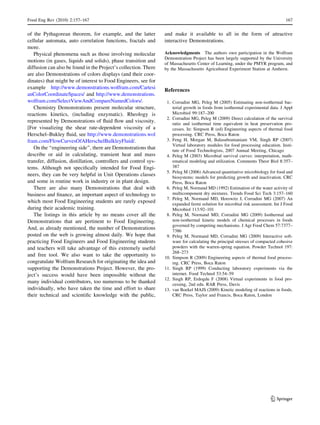
Fig. 11 Calculating the principal stresses and effective angle of
internal friction from experimental shear data of consolidated
cohesive powder specimens using the Warren-Spring equation as
the yield loci curve’s model
Fig. 12 Calculating the Reynolds number, friction factor and
frictional pressure drop in laminar and turbulent flows through a pipe
166 Food Eng Rev (2010) 2:157–167
123

11. of the Pythagorean theorem, for example, and the latter
cellular automata, auto correlation functions, fractals and
more.
Physical phenomena such as those involving molecular
motions (in gases, liquids and solids), phase transition and
diffusion can also be found in the Project’s collection. There
are also Demonstrations of colors displays (and their coor-
dinates) that might be of interest to Food Engineers, see for
example http://www.demonstrations.wolfram.com/Cartesi
anColorCoordinateSpaces/ and http://www.demonstrations.
wolfram.com/SelectViewAndCompareNamedColors/.
Chemistry Demonstrations present molecular structure,
reactions kinetics, (including enzymatic). Rheology is
represented by Demonstrations of fluid flow and viscosity.
[For visualizing the shear rate-dependent viscosity of a
Herschel–Bukley fluid, see http://www.demonstrations.wol
fram.com/FlowCurvesOfAHerschelBulkleyFluid/.
On the ‘‘engineering side’’, there are Demonstrations that
describe or aid in calculating, transient heat and mass
transfer, diffusion, distillation, controllers and control sys-
tems. Although not specifically intended for Food Engi-
neers, they can be very helpful in Unit Operations classes
and some in routine work in industry or in plant design.
There are also many Demonstrations that deal with
business and finance, an important aspect of technology to
which most Food Engineering students are rarely exposed
during their academic training.
The listings in this article by no means cover all the
Demonstrations that are pertinent to Food Engineering.
And, as already mentioned, the number of Demonstrations
posted on the web is growing almost daily. We hope that
practicing Food Engineers and Food Engineering students
and teachers will take advantage of this extremely useful
and free tool. We also want to take the opportunity to
congratulate Wolfram Research for originating the idea and
supporting the Demonstrations Project. However, the pro-
ject’s success would have been impossible without the
many individual contributors, too numerous to be thanked
individually, who have taken the time and effort to share
their technical and scientific knowledge with the public,
and make it available to all in the form of attractive
interactive Demonstrations.
Acknowledgments The authors own participation in the Wolfram
Demonstration Project has been largely supported by the University
of Massachusetts Center of Learning, under the PMYR program, and
by the Massachusetts Agricultural Experiment Station at Amherst.
References
1. Corradini MG, Peleg M (2005) Estimating non-isothermal bac-
terial growth in foods from isothermal experimental data. J Appl
Microbiol 99:187–200
2. Corradini MG, Peleg M (2009) Direct calculation of the survival
ratio and isothermal time equivalent in heat preservation pro-
cesses. In: Simpson R (ed) Engineering aspects of thermal food
processing. CRC Press, Boca Raton
3. Feng H, Morgan M, Balasubramaniam VM, Singh RP (2007)
Virtual laboratory modules for food processing education. Insti-
tute of Food Technologists, 2007 Annual Meeting, Chicago
4. Peleg M (2003) Microbial survival curves: interpretation, math-
ematical modeling and utilization. Comments Theor Biol 8:357–
387
5. Peleg M (2006) Advanced quantitative microbiology for food and
biosystems: models for predicting growth and inactivation. CRC
Press, Boca Raton
6. Peleg M, Normand MD (1992) Estimation of the water activity of
multicomponent dry mixtures. Trends Food Sci Tech 3:157–160
7. Peleg M, Normand MD, Horowitz J, Corradini MG (2007) An
expanded fermi solution for microbial risk assessment. Int J Food
Microbiol 113:92–101
8. Peleg M, Normand MD, Corradini MG (2009) Isothermal and
non-isothermal kinetic models of chemical processes in foods
governed by competing mechanisms. J Agr Food Chem 57:7377–
7386
9. Peleg M, Normand MD, Corradini MG (2009) Interactive soft-
ware for calculating the principal stresses of compacted cohesive
powders with the warren-spring equation. Powder Technol 197:
268–273
10. Simpson R (2009) Engineering aspects of thermal food process-
ing. CRC Press, Boca Raton
11. Singh RP (1999) Conducting laboratory experiments via the
internet. Food Technol 53:54–59
12. Singh RP, Erdogdu F (2008) Virtual experiments in food pro-
cessing, 2nd edn. RAR Press, Davis
13. van Boekel MAJS (2009) Kinetic modeling of reactions in foods.
CRC Press, Taylor and Francis, Boca Raton, London
Food Eng Rev (2010) 2:157–167 167
123