DSP

1. Structures for Discrete-Time Systems
Quote of the Day
Today's scientists have substituted mathematics for
experiments, and they wander off through equation
after equation, and eventually build a structure which
has no relation to reality.
Nikola Tesla
Content and Figures are from Discrete-Time Signal Processing, 2e by Oppenheim, Shafer, and Buck, ©1999-2000 Prentice Hall Inc.

2. Copyright (C) 2005 Güner Arslan 351M Digital Signal Processing 2
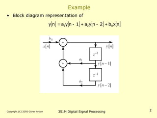
Example
• Block diagram representation of
       
n
x
b
2
n
y
a
1
n
y
a
n
y 0
2
1 





3. Copyright (C) 2005 Güner Arslan 351M Digital Signal Processing 3
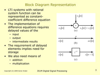
Block Diagram Representation
• LTI systems with rational
system function can be
represented as constant-
coefficient difference equation
• The implementation of
difference equations requires
delayed values of the
– input
– output
– intermediate results
• The requirement of delayed
elements implies need for
storage
• We also need means of
– addition
– multiplication

4. Copyright (C) 2005 Güner Arslan 351M Digital Signal Processing 4
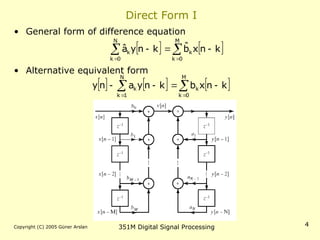
Direct Form I
• General form of difference equation
• Alternative equivalent form
   

 




M
0
k
k
N
0
k
k k
n
x
b̂
k
n
y
â
     

 





M
0
k
k
N
1
k
k k
n
x
b
k
n
y
a
n
y

5. Copyright (C) 2005 Güner Arslan 351M Digital Signal Processing 5
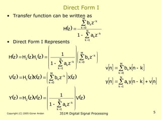
Direct Form I
• Transfer function can be written as
• Direct Form I Represents
 







 N
1
k
k
k
M
0
k
k
k
z
a
1
z
b
z
H
     
       
       
z
V
z
a
1
1
z
V
z
H
z
Y
z
X
z
b
z
X
z
H
z
V
z
b
z
a
1
1
z
H
z
H
z
H
N
1
k
k
k
2
M
0
k
k
k
1
M
0
k
k
k
N
1
k
k
k
1
2




























































   
     
n
v
k
n
y
a
n
y
k
n
x
b
n
v
N
1
k
k
M
0
k
k










6. Copyright (C) 2005 Güner Arslan 351M Digital Signal Processing 6
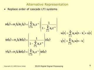
Alternative Representation
• Replace order of cascade LTI systems
     
       
       
z
W
z
b
z
W
z
H
z
Y
z
X
z
a
1
1
z
X
z
H
z
W
z
a
1
1
z
b
z
H
z
H
z
H
M
0
k
k
k
1
N
1
k
k
k
2
N
1
k
k
k
M
0
k
k
k
2
1




























































     
   









M
0
k
k
N
1
k
k
k
n
w
b
n
y
n
x
k
n
w
a
n
w

7. Copyright (C) 2005 Güner Arslan 351M Digital Signal Processing 7
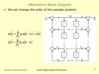
Alternative Block Diagram
• We can change the order of the cascade systems
     
   









M
0
k
k
N
1
k
k
k
n
w
b
n
y
n
x
k
n
w
a
n
w

8. Copyright (C) 2005 Güner Arslan 351M Digital Signal Processing 8
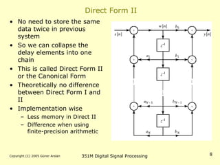
Direct Form II
• No need to store the same
data twice in previous
system
• So we can collapse the
delay elements into one
chain
• This is called Direct Form II
or the Canonical Form
• Theoretically no difference
between Direct Form I and
II
• Implementation wise
– Less memory in Direct II
– Difference when using
finite-precision arithmetic

9. Copyright (C) 2005 Güner Arslan 351M Digital Signal Processing 9
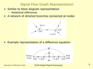
Signal Flow Graph Representation
• Similar to block diagram representation
– Notational differences
• A network of directed branches connected at nodes
• Example representation of a difference equation

10. Copyright (C) 2005 Güner Arslan 351M Digital Signal Processing 10
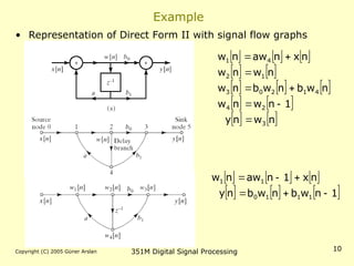
Example
• Representation of Direct Form II with signal flow graphs
     
   
     
   
   
n
w
n
y
1
n
w
n
w
n
w
b
n
w
b
n
w
n
w
n
w
n
x
n
aw
n
w
3
2
4
4
1
2
0
3
1
2
4
1








     
     
1
n
w
b
n
w
b
n
y
n
x
1
n
aw
n
w
1
1
1
0
1
1







11. Copyright (C) 2005 Güner Arslan 351M Digital Signal Processing 11
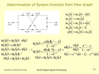
Determination of System Function from Flow Graph
     
   
     
   
     
n
w
n
w
n
y
1
n
w
n
w
n
x
n
w
n
w
n
w
n
w
n
x
n
w
n
w
4
2
3
4
2
3
1
2
4
1










     
   
     
   
     
z
W
z
W
z
Y
z
z
W
z
W
z
X
z
W
z
W
z
W
z
W
z
X
z
W
z
W
4
2
1
3
4
2
3
1
2
4
1










    
     
     
z
W
z
W
z
Y
z
1
1
z
z
X
z
W
z
1
1
z
z
X
z
W
4
2
1
1
4
1
1
2
















   
 
     
n
u
1
n
u
n
h
z
1
z
z
X
z
Y
z
H
1
n
1
n
1
1
















12. Copyright (C) 2005 Güner Arslan 351M Digital Signal Processing 12
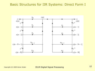
Basic Structures for IIR Systems: Direct Form I

13. Copyright (C) 2005 Güner Arslan 351M Digital Signal Processing 13
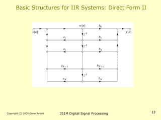
Basic Structures for IIR Systems: Direct Form II

14. Copyright (C) 2005 Güner Arslan 351M Digital Signal Processing 14
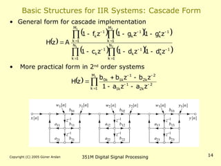
Basic Structures for IIR Systems: Cascade Form
• General form for cascade implementation
• More practical form in 2nd
order systems
 
    
    






















 2
1
2
1
N
1
k
1
k
1
k
N
1
k
1
k
M
1
k
1
k
1
k
M
1
k
1
k
z
d
1
z
d
1
z
c
1
z
g
1
z
g
1
z
f
1
A
z
H
  










1
M
1
k
2
k
2
1
k
1
2
k
2
1
k
1
k
0
z
a
z
a
1
z
b
z
b
b
z
H

15. Copyright (C) 2005 Güner Arslan 351M Digital Signal Processing 15
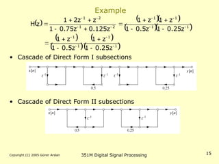
Example
• Cascade of Direct Form I subsections
• Cascade of Direct Form II subsections
    
  
 
 
 
 
1
1
1
1
1
1
1
1
2
1
2
1
z
25
.
0
1
z
1
z
5
.
0
1
z
1
z
25
.
0
1
z
5
.
0
1
z
1
z
1
z
125
.
0
z
75
.
0
1
z
z
2
1
z
H




























16. Copyright (C) 2005 Güner Arslan 351M Digital Signal Processing 16
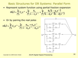
Basic Structures for IIR Systems: Parallel Form
• Represent system function using partial fraction expansion
• Or by pairing the real poles
   
  
 
  














P P
P N
1
k
N
1
k
1
k
1
k
1
k
k
1
k
k
N
0
k
k
k
z
d
1
z
d
1
z
e
1
B
z
c
1
A
z
C
z
H
  
 










S
P N
1
k
2
k
2
1
k
1
1
k
1
k
0
N
0
k
k
k
z
a
z
a
1
z
e
e
z
C
z
H

17. Copyright (C) 2005 Güner Arslan 351M Digital Signal Processing 17
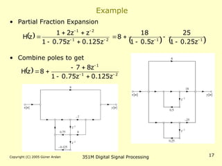
Example
• Partial Fraction Expansion
• Combine poles to get
 
   
1
1
2
1
2
1
z
25
.
0
1
25
z
5
.
0
1
18
8
z
125
.
0
z
75
.
0
1
z
z
2
1
z
H 















  2
1
1
z
125
.
0
z
75
.
0
1
z
8
7
8
z
H 









18. Copyright (C) 2005 Güner Arslan 351M Digital Signal Processing 18
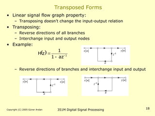
Transposed Forms
• Linear signal flow graph property:
– Transposing doesn’t change the input-output relation
• Transposing:
– Reverse directions of all branches
– Interchange input and output nodes
• Example:
– Reverse directions of branches and interchange input and output
  1
az
1
1
z
H 



19. Copyright (C) 2005 Güner Arslan 351M Digital Signal Processing 19
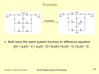
Example
Transpose
• Both have the same system function or difference equation
           
2
n
x
b
1
n
x
b
n
x
b
2
n
y
a
1
n
y
a
n
y 2
1
0
2
1 









20. Copyright (C) 2005 Güner Arslan 351M Digital Signal Processing 20
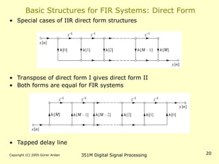
Basic Structures for FIR Systems: Direct Form
• Special cases of IIR direct form structures
• Transpose of direct form I gives direct form II
• Both forms are equal for FIR systems
• Tapped delay line

21. Copyright (C) 2005 Güner Arslan 351M Digital Signal Processing 21
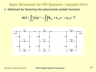
Basic Structures for FIR Systems: Cascade Form
• Obtained by factoring the polynomial system function
     
 
 







M
0
n
M
1
k
2
k
2
1
k
1
k
0
n
S
z
b
z
b
b
z
n
h
z
H

22. Copyright (C) 2005 Güner Arslan 351M Digital Signal Processing 22
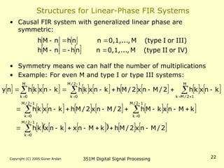
Structures for Linear-Phase FIR Systems
• Causal FIR system with generalized linear phase are
symmetric:
• Symmetry means we can half the number of multiplications
• Example: For even M and type I or type III systems:
   
    IV)
or
II
(type
M
0,1,...,
n
n
h
n
M
h
III)
or
I
(type
M
0,1,...,
n
n
h
n
M
h







                 
           
     
     
2
/
M
n
x
2
/
M
h
k
M
n
x
k
n
x
k
h
k
M
n
x
k
M
h
2
/
M
n
x
2
/
M
h
k
n
x
k
h
k
n
x
k
h
2
/
M
n
x
2
/
M
h
k
n
x
k
h
k
n
x
k
h
n
y
1
2
/
M
0
k
1
2
/
M
0
k
1
2
/
M
0
k
M
1
2
/
M
k
1
2
/
M
0
k
M
0
k









































23. Copyright (C) 2005 Güner Arslan 351M Digital Signal Processing 23
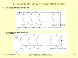
Structures for Linear-Phase FIR Systems
• Structure for even M
• Structure for odd M