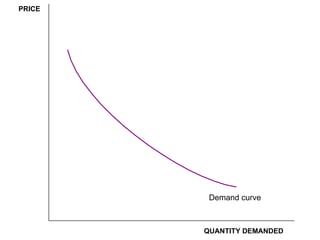
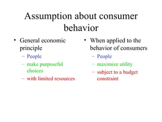
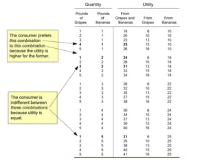
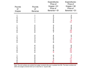
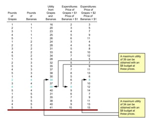
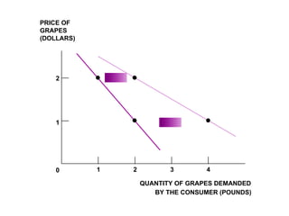
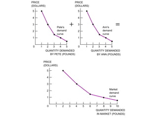
The document provides an overview of concepts that will be covered related to demand and supply, including: 1) It begins with an introduction of the derivation of the demand curve from the perspective of individual consumers and their preferences between goods subject to a budget constraint. 2) It then discusses how the aggregation of individual demand curves results in the market demand curve. 3) The document outlines how understanding demand curves can help explain the functioning of competitive markets and determine the position and sensitivity of demand.

2. Preview of 4 Coming Attractions
• Today: Derivation of the Demand Curve
– Consumers (Buyers)
• Next: Derivation of the Supply Curve
– Firms (Sellers)
• Later: Double Auction Market
– Buyers and and sellers come together
• Still later: Competitive Equilibrium Model

3. 05_01 PRICE
Demand curve
QUANTITY DEMANDED

4. Why study the derivation of the
demand curve?
• Helps explain why a competitive market
works well.
• Helps determine the position of the demand
curve and the sensitivity of quantity
demanded to price.

5. A brief digression on elasticity
• Elasticity is a measure of how sensitive one
variable (e.g. quantity demanded) is to
another variable (e.g. price).
• Definition: the price elasticity of demand is
the percentage change in quantity
demanded divided by the percentage change
in price e = (%D Q)/(%DP)

6. Where we are going
• Start with an individual consumer
– maybe you, maybe me, but could be anyone
• Derive demand curve for that individual
– focus on marginal utility or marginal benefit
• Add up demand curves for many such
individuals to get market demand curve

7. Assumption about consumer
behavior
• General economic
principle
– People
– make purposeful
choices
– with limited resources
• When applied to the
behavior of consumers
– People
– maximize utility
– subject to a budget
constraint

8. Utility: a numerical indicator of
preferences
• Marginal Utility
• Diminishing Marginal Utility

9. 05_03T Quantity Utility
Pounds Pounds From
of of Grapes and From From
Grapes Bananas Bananas Grapes Bananas
1 1 16 6 10
2 1 20 10 10
3 1 23 13 10
4 1 25 15 10
5 1 26 16 10
1 2 24 6 18
2 2 28 10 18
3 2 31 13 18
4 2 33 15 18
5 2 34 16 18
1 3 28 6 22
2 3 32 10 22
3 3 35 13 22
4 3 37 15 22
5 3 38 16 22
1 4 30 6 24
2 4 34 10 24
3 4 37 13 24
4 4 39 15 24
5 4 40 16 24
1 5 31 6 25
2 5 35 10 25
3 5 38 13 25
4 5 40 15 25
5 5 41 16 25
The consumer prefers
this combination
to this combination
because the utility is
higher for the former.
The consumer is
indifferent between
these combinations
because utility is
equal.

10. 05_04T
Expenditures:
Price of
Grapes = $1
Price of
Bananas = $1
Pounds
of
Bananas
Expenditures:
Price of
Grapes = $2
Price of
Bananas = $1
Pounds
of
Grapes
1 1 2 3
2 1 3 5
3 1 4 7
4 1 5
9
5 1 6
11
1 2 3 4
2 2 4 6
3 2 5 8
4 2 6
10
5 2 7
12
1 3 4 5
2 3 5 7
3 3 6
9
4 3 7
11
5 3 8
13
1 4 5 6
2 4 6 8
3 4 7
10
4 4 8
12
5 4
9 14
1 5 6 7
2 5 7
9
3 5 8
11
4 5
9 13
5 5
10 15
Note: The red numbers are outside the budget constraint (the sum is greater than $8). The black numbers are
within the budget constraint (the sum is less than or equal to $8).

11. 05_05T
Expenditures:
Price of
Grapes = $1
Price of
Bananas = $1
Pounds
of
Bananas
Expenditures:
Price of
Grapes = $2
Price of
Bananas = $1
Pounds
of
Grapes
Utility
from
Grapes
and
Bananas
1 1 16 2 3
2 1 20 3 5
3 1 23 4 7
4 1 25 5 9
5 1 26 6 11
1 2 24 3 4
2 2 28 4 6
3 2 31 5 8
4 2 33 6 10
5 2 34 7 12
1 3 28 4 5
2 3 32 5 7
3 3 35 6 9
4 3 37 7 11
5 3 38 8 13
1 4 30 5 6
2 4 34 6 8
3 4 37 7 10
4 4 39 8 12
5 4 40 9 14
1 5 31 6 7
2 5 35 7 9
3 5 38 8 11
4 5 40 9 13
5 5 41 10 15
A maximum utility
of 39 can be
obtained with an
$8 budget at
these prices.
A maximum utility
of 34 can be
obtained with an
$8 budget at
these prices.

12. 05_C
PRICE OF
GRAPES
(DOLLARS)
2
1
0
1 2 3 4
QUANTITY OF GRAPES DEMANDED
BY THE CONSUMER (POUNDS)

13. Marginal conditions for utility
maximization
• Ratio of marginal utilities equals ratio of
prices for any two goods
• (MUG/MUB) = (PG/PB)
• Explanation of Diamond Water Paradox
– First pointed out by Adam Smith

14. The “willingness to pay”
approach
Amount
of X
Willingness
to pay
Marginal
Beneift
0 $0 ---
1 $4 $4
2 $7 $3
3 $9 $2
4 $10 $1

15. 05_05
1 2 3 4 5
5
4
3
2
1
0
QUANTITY DEMANDED (POUNDS)
DOLLARS

16. An Important Conclusion:
MB = P
• The consumer chooses an amount such that
the marginal benefit (MB) equals price (P)
• When I see a demand curve, I think of the
marginal benefit to consumers
• WGAD: Why do economists put the
quantity on the horizontal axis?

17. Consumer Surplus
• Willingness to pay is usually greater than
the price
– for example my willingness to pay for a pair of
eyeglasses is much more than the price
• Consumer surplus is the area under the
demand curve and above the price

18. Market Demand Curve
• Consider all consumers in the market
• Add up quantity demanded by all
individuals at each price to get market
demand
• Add horizontally

19. 05_06
5
4
3
2
1
0 1 2 3 4 5
5
4
3
2
1
Ann's
demand
curve
0 1 2 3 4 5
QUANTITY DEMANDED
5
4
3
2
1
BY PETE (POUNDS)
QUANTITY DEMANDED
BY ANN (POUNDS)
0 1 2 3 4 5 6 7 8 9 10
QUANTITY DEMANDED
IN MARKET (POUNDS)
PRICE
(DOLLARS)
PRICE
(DOLLARS)
PRICE
(DOLLARS)
Market
demand
curve
Pete's
demand
curve
+ =