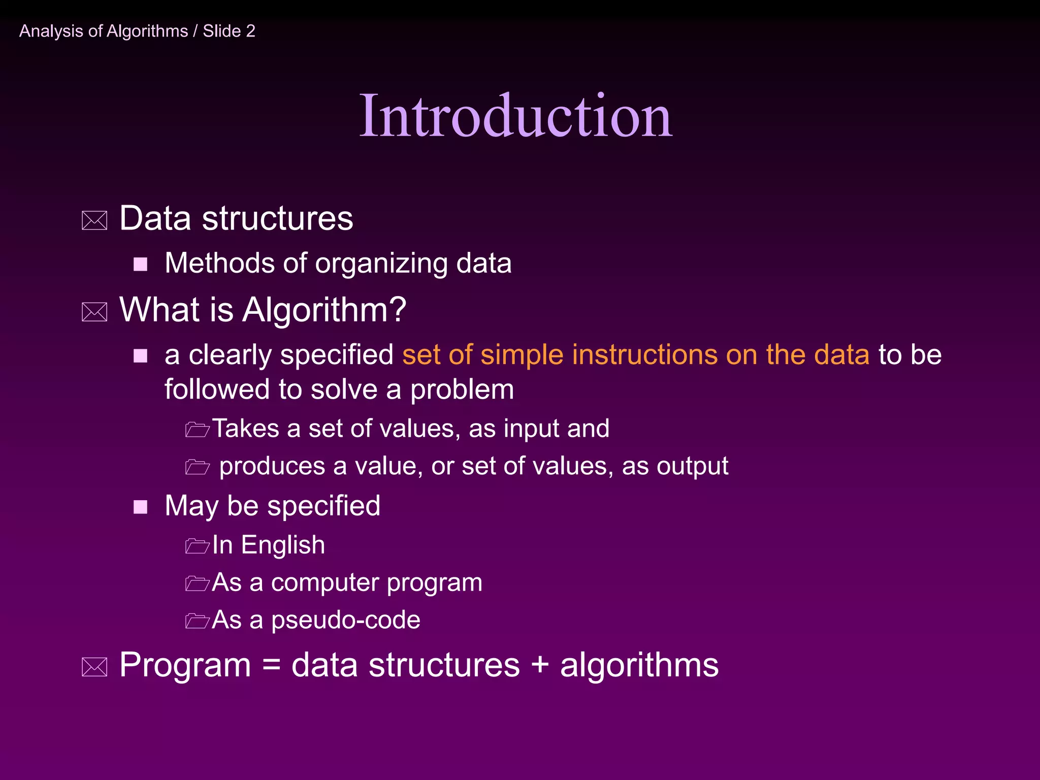
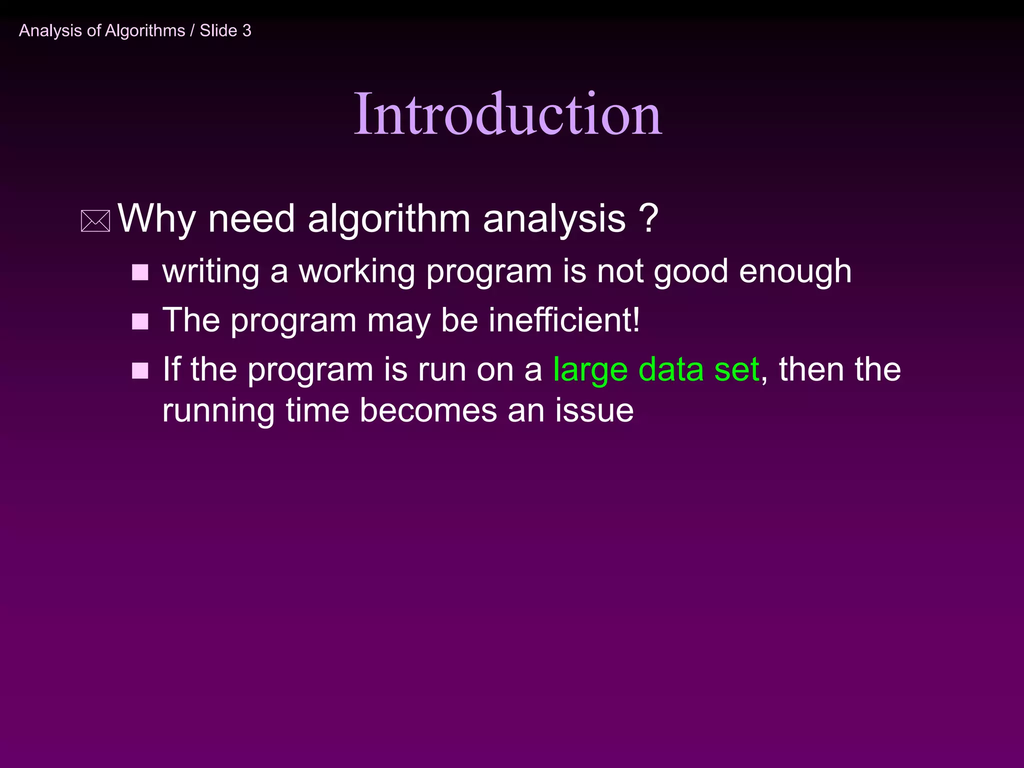
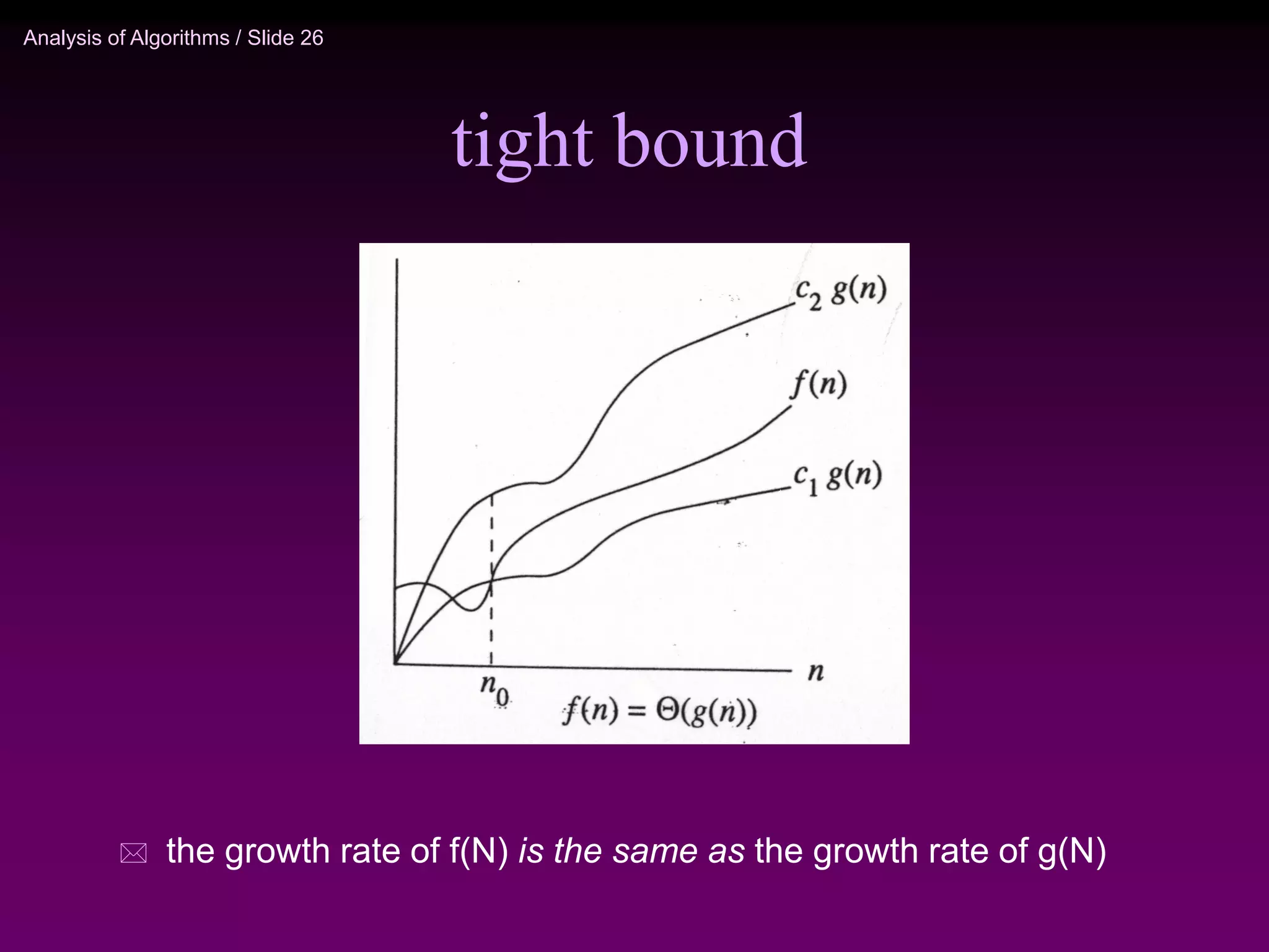
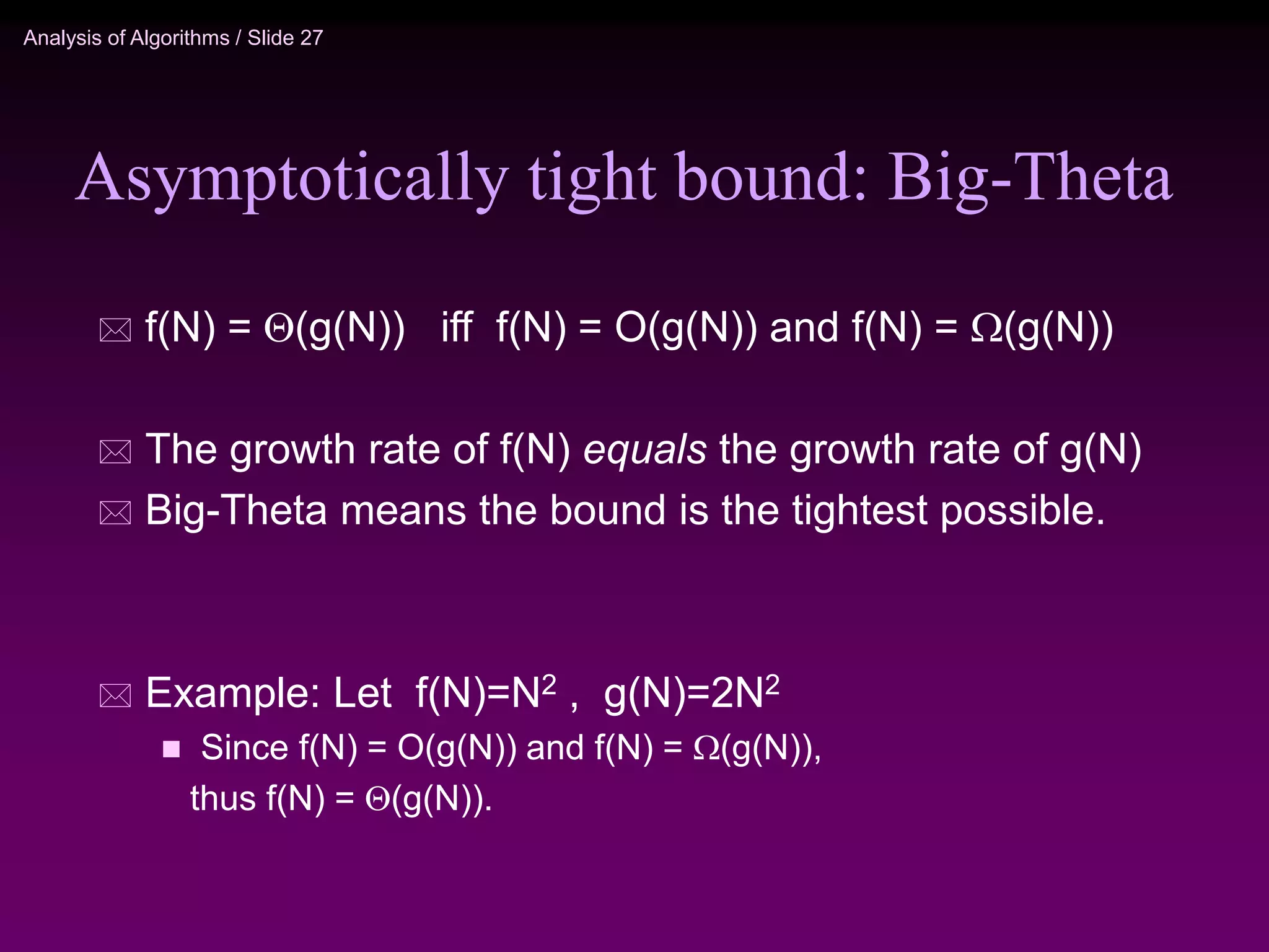
This document provides an introduction to algorithm analysis. It discusses why algorithm analysis is important, as an inefficient program may have poor running time even if it is functionally correct. It introduces different algorithm analysis approaches like empirical, simulational, and analytical. Key concepts in algorithm analysis like worst-case, average-case, and best-case running times are explained. Different asymptotic notations like Big-O, Big-Omega, and Big-Theta that are used to describe the limiting behavior of functions are also introduced along with examples. Common algorithms like linear search and binary search are analyzed to demonstrate how to determine the time complexity of algorithms.


![Analysis of Algorithms / Slide 33
O(N)
// Given an array of ‘size’ in increasing order, find ‘x’
int linearsearch(int* a[], int size,int x) {
int low=0, high=size-1;
for (int i=0; i<size;i++)
if (a[i]==x) return i;
return -1;
}
Linear search:](https://image.slidesharecdn.com/analysis-220918045142-d9b368c7/75/analysis-ppt-33-2048.jpg)
![Analysis of Algorithms / Slide 34
int bsearch(int* a[],int size,int x) {
int low=0, high=size-1;
while (low<=higt) {
int mid=(low+high)/2;
if (a[mid]<x)
low=mid+1;
else if (x<a[mid])
high=mid-1;
else return mid;
}
return -1
}
Iterative binary search:](https://image.slidesharecdn.com/analysis-220918045142-d9b368c7/75/analysis-ppt-34-2048.jpg)
![Analysis of Algorithms / Slide 35
int bsearch(int* a[],int size,int x) {
int low=0, high=size-1;
while (low<=higt) {
int mid=(low+high)/2;
if (a[mid]<x)
low=mid+1;
else if (x<a[mid])
high=mid-1;
else return mid;
}
return -1
}
Iterative binary search:
n=high-low
n_i+1 <= n_i / 2
i.e. n_i <= (N-1)/2^{i-1}
N stops at 1 or below
there are at most 1+k iterations, where k is the smallest such
that (N-1)/2^{k-1} <= 1
so k is at most 2+log(N-1)
O(log N)](https://image.slidesharecdn.com/analysis-220918045142-d9b368c7/75/analysis-ppt-35-2048.jpg)
![Analysis of Algorithms / Slide 36
O(1)
T(N/2)
int bsearch(int* a[],int low, int high, int x) {
if (low>high) return -1;
else int mid=(low+high)/2;
if (x=a[mid]) return mid;
else if(a[mid]<x)
bsearch(a,mid+1,high,x);
else bsearch(a,low,mid-1);
}
O(1)
Recursive binary search:
1
)
2
(
)
(
1
)
1
(
N
T
N
T
T](https://image.slidesharecdn.com/analysis-220918045142-d9b368c7/75/analysis-ppt-36-2048.jpg)

![Analysis of Algorithms / Slide 41
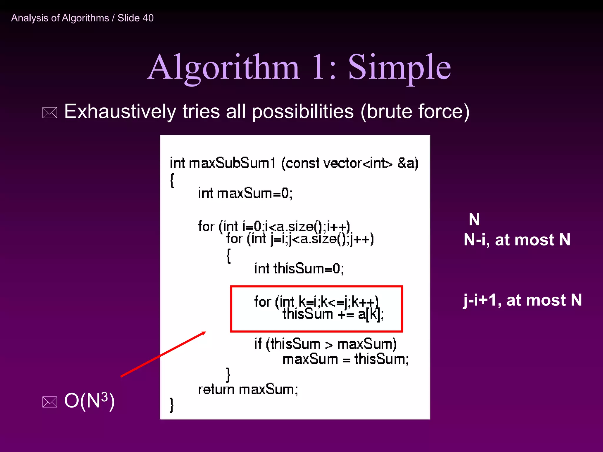
Algorithm 2: improved
N
N-i, at most N
O(N^2)
// Given an array from left to right
int maxSubSum(const int* a[], const int size) {
int maxSum = 0;
for (int i=0; i< size; i++) {
int thisSum =0;
for (int j = i; j < size; j++) {
thisSum += a[j];
if(thisSum > maxSum)
maxSum = thisSum;
}
}
return maxSum;
}](https://image.slidesharecdn.com/analysis-220918045142-d9b368c7/75/analysis-ppt-41-2048.jpg)
![Analysis of Algorithms / Slide 44
O(1)
T(N/2)
O(N)
O(1)
T(N/2)
// Given an array from left to right
int maxSubSum(a,left,right) {
if (left==right) return a[left];
else
mid=(left+right)/2
maxLeft=maxSubSum(a,left,mid);
maxRight=maxSubSum(a,mid+1,right);
maxLeftBorder=0; leftBorder=0;
for(i = mid; i>= left, i--) {
leftBorder += a[i];
if (leftBorder>maxLeftBorder)
maxLeftBorder=leftBorder;
}
// same for the right
maxRightBorder=0; rightBorder=0;
for … {
}
return max3(maxLeft,maxRight, maxLeftBorder+maxRightBorder);
}
O(N)](https://image.slidesharecdn.com/analysis-220918045142-d9b368c7/75/analysis-ppt-44-2048.jpg)