Lecture 1 Modern Control Theory- Introduction

Modern Control Theory
Chapter 1:
Introduction to Control
System
Dr. RALPH GERARD B. SANGALANG
College of Engineering Graduate School
BATANGAS STATE UNIVERSITY
The National Engineering University

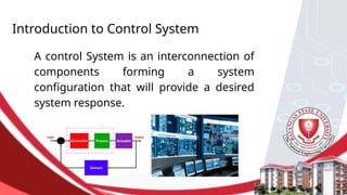
Introduction to Control System
A control System is an interconnection of
components forming a system
configuration that will provide a desired
system response.

Example:
Temperature Control System

Example:
Chemical Process
Control

Further Example:
• Cruise Control in vehicle
• Active suspensions system in vehicle
• Robotics
• Energy system
• Battery Charging System

p
Representation of a System
Process
Input Output
u y

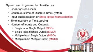
System can, in general be classified as:
• Linear or Non-Linear
• Continuous time or Discrete Time System
• Input-output relation or State-space representation
• Time invariant or Time varying
• Number of Inputs and Outputs:
⚬ Single Input Single Output (SISO)
⚬ Single Input Multiple Output (SIMO)
⚬ Multiple Input Single Output (MISO)
⚬ Multiple Input Multiple Output (MIMO)

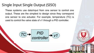
Single Input Single Output (SISO)
These systems use data/input from one sensor to control one
output. These are the simplest to design since they correspond
one sensor to one actuator. For example, temperature (TC) is
used to control the valve state of v1 through a PID controller.

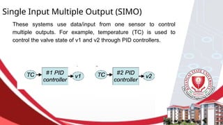
Single Input Multiple Output (SIMO)
These systems use data/input from one sensor to control
multiple outputs. For example, temperature (TC) is used to
control the valve state of v1 and v2 through PID controllers.

Multiple Input Single Output (MISO)
These systems use data/input from multiple sensors to control
one ouput. For example, a cascade controller can be considered
MISO. Temperature (TC) is used in a PID controller (#1) to
determine a flow rate set point i.e. FCset. With the FCset and FC
controller, they are used to control the valve state of v1 through a
PID controller (#2).

Multiple Input Multiple Output (MIMO)
These systems use data/input from multiple sensors to control multiple
outputs. These are usually the hardest to design since multiple sensor
data is integrated to coordinate multiple actuators. For example, flow rate
(FC) and temperature (TC) are used to control multiple valves (v1, v2,
and v3). Often, MIMO systems are not PID controllers but rather
designed for a specific situation.

Open Loop Control System
An open-loop control system utilizes a controller or control actuator to
obtain a desired response.
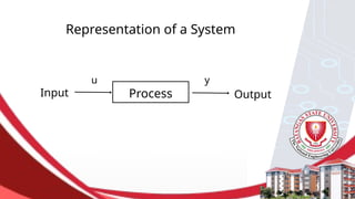
p
Process Output
u y
y
p
Actuating
device
Desire response

Example:
Open Loop Control of a
turntable

p
p
p
Close Loop Control System
The closed-loop control system employs the measurement of actual
output and modification of the input to the process through feedback of
actual output and thereby maintain the output at a required value.
Process
Actual Output
response
Controller
+
-
Desire Output
Response
Measurement
Device

Example:
Close Loop Control of a
turntable

Linear System
A linear system is a system that satisfies the principle of superposition

State Space model
a representation of the dynamics of an Nth order system as a first order
differential equation in an N-vector, which is called the state.
• Convert the Nth order differential equation that governs the dy
namics into N first-order differential equations

State Space Model
Classic Example:
second order mass-spring system

State-Space Linear System
A continuous-time state-space linear system is defined by the following two
equations:
The Signals
are called the input, state, and output of the system. The first-order
differential equation (1.1a) is called the state equation and (1.1b) is called the
output equation. The equations express an input-output relationship between
the input signal u(·) and the output signal y(·). For a given input u(·), we need
to solve the state equation to determine the state x(·) and then replace it in
the output equation to obtain the output y(·).

When the input signal u takes scalar values (k = 1), the system is called
single input (SI); otherwise, it is called multiple input (MI). When the output
signal y takes scalar values (m = 1) the system is called single output (SO);
otherwise, it is called multiple output (MO).
When there is no state equation (n = 0) and we have simply
the system is called memoryless.
When all the matrices A(t), B(t), C(t), D(t) are constant t 0
∀ ≥ , the systembis
called a linear time-invariant (LTI) system. In the general case, (1.1) is
called a linear time-varying (LTV) system to emphasize that time invariance is
not being assumed.

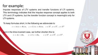
for example:
Impulse responses of LTV systems and transfer functions of LTI systems.
This terminology indicates that the impulse response concept applies to both
LTV and LTI systems, but the transfer function concept is meaningful only for
LTI systems.
To keep formulas short, in the following we abbreviate to
and in the time-invariant case, we further shorten this to

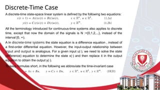
A In discrete-time systems the state equation is a difference equation , instead of
a first-order differential equation. However, the input-output relationship between
input and output is analogous. For a given input u(·), we need to solve the state
(difference) equation to determine the state x(·) and then replace it in the output
equation to obtain the output y(·).
Discrete-Time Case
A discrete-time state-space linear system is defined by the following two equations:
All the terminology introduced for continuous-time systems also applies to discrete
time, except that now the domain of the signals is N :={0,1,2,...}, instead of the
interval [0, ∞).
To keep formulas short, in the following we abbreviate the time-invariant case

State-Space Systems in MATLAB
MATLAB has several commands to create and manipulate LTI systems.
The command sys_ss=ss(A,B,C,D) assigns to sys_ss a continuous-time LTI state-space
MATLAB system of the form.

Optionally, one can specify the names of the inputs, outputs, and state to be used in
subsequent plots as follows:
The number of elements in the bracketed lists must match the number of inputs, outputs,
and state variables.
For discrete-time systems, one should instead use the command sys ss=ss(A,
B,C,D,Ts),where Ts is the sampling time, or-1 if one does not want to specify it.

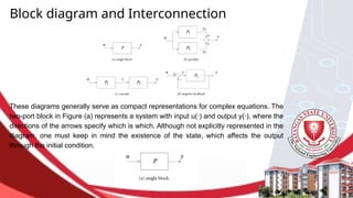
These diagrams generally serve as compact representations for complex equations. The
two-port block in Figure (a) represents a system with input u(·) and output y(·), where the
directions of the arrows specify which is which. Although not explicitly represented in the
diagram, one must keep in mind the existence of the state, which affects the output
through the initial condition.
Block diagram and Interconnection

Interconnections of block diagrams are especially useful to highlight special structures
in state-space equations.
Lets assume that the blocks P1 and P2 that appear in block diagram above are the two
LTI systems
The general procedure to obtain the state-space for an interconnection consists of
stacking the states of the individual subsystems in a tall vector x and computing ˙ x using
the state and output equations of the individual blocks. The output equation is also
obtained from the output equations of the subsystems.

In the block diagram letter (b) we have u = u1 = u2 and y = y1 + y2, which corresponds
to a parallel interconnection. This figure represents the LTI system
with state The parallel structure is responsible for the block-diagonal
structure in the matrix
A block-diagonal structure in this matrix indicates that the state-space system can be
decomposed as the parallel of two state-space systems with smaller states.

In Block Diagram Letter (c) we have u = u1, y = y2, and z = y1 = u2, which corresponds
to a cascade interconnection. This figure represents the LTI system
with state
triangular structure in the matrix
The cascade structure is responsible for the block
,and,infact,ablock-triangularstructure
in this matrix indicates that the state-space system can be decomposed as a cas cade of
two state-space systems with smaller states.

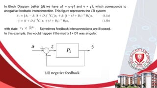
In Block Diagram Letter (d) we have u1 = u−y1 and y = y1, which corresponds to
anegative feedback interconnection. This figure represents the LTI system
with state Sometimes feedback interconnections are ill-posed.
In this example, this would happen if the matrix I + D1 was singular.

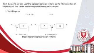
Block diagrams are also useful to represent complex systems as the interconnection of
simple blocks. This can be seen through the following two examples:
1. The LTI system
Block diagram representation systems.

2. Consider the LTI system
Writing these equations as
and
where z := x2 +u, we conclude that (1.4) can be viewed as the block diagram in
Figure 1.2(b), where P3 corresponds to the LTI system (1.5) with input u and
output y2 and P4 corresponds to the LTI systems (1.6) with input z and output y.

THANK YOU!!!
College of Engineering Graduate School
BATANGAS STATE UNIVERSITY
The National Engineering University

Lecture 1 Modern Control Theory- Introduction

More Related Content

Similar to Lecture 1 Modern Control Theory- Introduction

Recently uploaded

Lecture 1 Modern Control Theory- Introduction