The document provides an overview of data preprocessing techniques for data mining. It discusses how data is typically represented as a table with rows and columns, where each row is a data object represented as a vector of attribute values. It describes different types of attributes like nominal, ordinal, interval, and ratio attributes, and the possible operations that can be performed on each attribute type. Preprocessing techniques must be compatible with the attribute types in the data. The document emphasizes that understanding the data type is important for choosing appropriate data mining algorithms to apply.

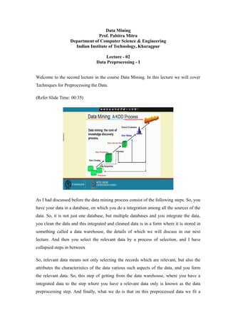
1. Data Mining
Prof. Pabitra Mitra
Department of Computer Science & Engineering
Indian Institute of Technology, Kharagpur
Lecture - 02
Data Preprocessing - I
Welcome to the second lecture in the course Data Mining. In this lecture we will cover
Techniques for Preprocessing the Data.
(Refer Slide Time: 00:35)
As I had discussed before the data mining process consist of the following steps. So, you
have your data in a database, on which you do a integration among all the sources of the
data. So, it is not just one database, but multiple databases and you integrate the data,
you clean the data and this integrated and cleaned data is in a form where it is stored in
something called a data warehouse, the details of which we will discuss in our next
lecture. And then you select the relevant data by a process of selection, and I have
collapsed steps in between.
So, relevant data means not only selecting the records which are relevant, but also the
attributes the characteristics of the data various such aspects of the data, and you form
the relevant data. So, this step of getting from the data warehouse, where you have a
integrated data to the step where you have a relevant data only is known as the data
preprocessing step. And finally, what we do is that on this preprocessed data we fit a

2. mathematical model, which describes the patterns present in the data either association
rules or classification rules, we have a mathematical description of this clean data and
then we evaluate the patterns, evaluate the models and those evaluated and visualized
model which is usable by an human into some actionable form is what we call a
knowledge.
So, before going into the details of the mathematical modeling part, in this lecture we
will cover the preprocessing tasks, that you have to perform before you start the data
mining.
(Refer Slide Time: 02:52)
So, before describing what are the preprocessing steps, let me just clarify you once more
what exactly is we call as data what is what is the actual form of data, the computer
representation of data that we will be preprocessing. So, there are various forms of the
data one of the most popular form which we will use in most of the data mining
processes is in the form of a table. So, this table you see on the right is the basically your
data. So, as you can see that table is a two dimensional structure, it has some columns
and it has rows. Just like a irrational database system each of these columns represent
some measurements or some observations. For example, suppose I want a data mining
system to evaluate whether a person who has applied for a bank loan is a genuine person
or a fraud person a cheat person.

3. So, maybe this is our data mining talks that some bank has asked you to do it and each of
the rows. So, what we can do, we will do this data mining; that means, whether a person
is a cheat or a normal person, based on the previous history of cheats and non cheats and
this previous history is our data. That is our data that is what we will mining the all the is
a may be the bank so far granted say one lakh loans in this year. So, all this records of
this one lakh loan that has been granted or not granted in this year is our data. How do
you represent this data we represent it like a table, what does the table say? Each column
of the table is some fact or some characteristics of each of these loans, each of these loan
applications what are the characteristics.
For example one characteristic is where if I have given a loan whether the person has
refunded the loan returned back, the loan similarly what is the marital status single or
married. Similarly what is the tax the income tax the person has paid, taxable income the
person has paid. So, these three values somebody who has applied for a loan will write
down in the application and these values are my data, for that particular application for
that particular person. So, you can see that each row in this table is one loan application;
and the last column you can see it is also a variable and attribute, but it is what our
interest is to infer whether that person is cheat or a cheat yes or cheat no.
So, that is a special attribute, that we would like to infer or the output of our mining
algorithm. So, now, let us come to some terminology, each of the columns in this case a
loan application is a object it is a object, and each of these columns which are
measurements on that particular object are the attributes or the properties of that object.
So, examples may be may be the eye color of the person, may be some temperature of
some quantity.
So, this attributes have other names also, they are also sometimes known as variables,
they are also sometimes known as features, they are also some time known as inputs. So,
these are the variables or attributes and each of the rows are these attribute values for a
particular object and they are known as either records or samples or instances or cases or
entities each of this name are popular depending on the application.
One important thing to be noted is that this particular representation if we examine a row,
you can think of each row as a vector, whose components are this individual attribute
values. So, these vectors are also sometimes known as the object vector or the feature

4. vector a description a representation of the object in terms of a vector. What is the
dimension of the vector? The dimension of the vector is determined by the number of
attributes you have. So, if we have three attributes in this case, it is a three dimensional
vector and since every vector can also be represented for example, here every row except
for the last column can be represented as a three dimensional point, a point in a three
dimensional coordinate system. In general if you have n attributes every object can be
thought of as a point in a n dimensional coordinate system.
So, thus our data is nothing, but a collection of such vectors. So, a each vector is a n
dimensional feature vector or a attribute vector or a n dimensional point this is. So, this is
a this is I think very emptive and very common representation of the data, but what you
should keep in your mind when we do for the data mining is that you should understand
that, every input data every data object can be viewed as an n dimensional vector whose
components are the attributes or a n dimensional point equivalently an n dimensional
point. So, one of the advantage of this visualization is that, you can actually plot your
data on n dimensional coordinate system visualize them as points.
So, a collection all these loan applications over the past year may be one lakh can be
thought of as one lakh points in a three dimensional coordinate system. And once you do
that it helps us to visualize what the nature of the data is. So, now, the take away from
this slide is that your data will be usually represented as a table, where each row is a n
dimensional vector representing one object one instance of the data, when columns are
the coordinates of this n dimensional object which represent the attribute values or a
certain properties of these objects. Now the values that each of this attribute take can be
of the following type, it can be something called a nominal attribute nominal coming
from the word name.

5. (Refer Slide Time: 11:21)
That means it is just a symbol for example, the ID number of a bank account it is just a
number, it has it has no other meaning it is just a number I D number, eye color say black
or white or blue zip code the pin code of a place. So, these are just numbers these are
nominal values, these are just some identifiers. Why these are just symbols? Because
suppose a person has a bank account number say 1001; and another person has a bank I
Dnumber bank account number or a ID number say 1002 you cannot really say that the
person with 1002 is greater than the person with 1001, you cannot compare these values
they are just for example, my name is Pabitra Mitra and another person’s name is say
something else say Ram kumar.
So, it does not tell us about anything more besides our identified does not tell us that
Pabitra Mitra dictionary order is before Ram Kumar. So, he is greater than Ram Kumar
you cannot compare two names. So, these are just nominal values, the other type can be
ordinal attributes, where you can actually compare the values you can rank them, you
can ordinal comes from order. For example, you are rating a movie or a potato chips for
example, in a scale of 1 to 10 how good it is or how bad it is or if any product. So,
naturally these values 1234 they can now be compared 7 is greater than 5, 3 is worse
than ten whereas, ID number a person’s bank account number cannot be said that it is
less than the other or for example, say height of a person tall or medium or short you
know tall is greater than short.

6. So, you can actually compare ordinal values; the next type is what is called interval
valued attributes where the value represents some intervals for example, a date calendar
date it tells you that whether another date, if you have you say the date of loan
application the another date a loan application and loan granting dates these two dates
you can say that one is within the other it falls in the range of the other. So, you can say
that one belongs to this interval one does not belong to this interval. Similarly the
temperature in Celsius or Fahrenheit they are scales they basically represent a range of
value, the fourth type is what is known as a ratio attribute ratio attribute type, these are
like free numbers they can be anything.
For example a absolute scale in temperature a length a time some count of something,
they are neither interval they are free values you can do whatever you want to do with it
you can add them, you can multiply them you can compare them all the properties of the
previous attributes you can do to them.
(Refer Slide Time: 15:28)
Now, let us look at some properties of this attribute values we will. So, whenever we
have say- two objects having different attribute values. In this data mining process we
will like to perform some operation some kind of basic computation on these values what
are the computations? You can the simplest form is checking for distinguish whether two
values are same or they different equal to or not equal to just that is your universe, that is

7. the only option operation you can only comparison you can make whether they are equal
or they are not equal.
For example two names only thing I can do operation between two names is that, either it
is the same name or it is the different name no other you cannot make greater than less
than multiply two names has no meaning, only thing that has meaning is that whether
two names are same or are they different. A slightly more complex operation is the order
operation, you can check whether a value is greater than another value or less than
another value you can find their order relative order and then you have the addition or
subtraction operations, where you can add two values and finally, multiplication and
division operators. Now in in the different type of attribute values we discussed it is only
some of these operations that we can perform.
Let me for example, say you consider nominal values names account numbers; the only
operation you can do on them is check whether they are distinct or not no other you
cannot add them you cannot check their order nothing you can do. If it is a ordinal
attribute you can either check for distinctness whether they are identical or you can
check for their order whether one is greater say. For example, a movie rating seven either
it is same as another movie rating or it is better than another movie rating you can check
for order and distinguish. For interval value at distinct attributes where you have
intervals say date range or time range, you can do distinctness you can do order.
Whether the one has applied for a loan before another person, whether at the same time
or before that and you can add them also you can join two intervals and make larger
intervals you can add them also finally, for the ratio attributes you can perform any of
these four operations you can multiply them also. You can divide one length by another
length whereas, you cannot divide it date by another date.
So, the reason I am explaining this is that in your real life application, your table data
table that you get might contain attributes which are which might be any of these types,
they can be for example, consider a bank loan you have ordinal attributes which is the
bank account number you have order attributes, which is maybe the bank the bank
balance of the person, you have interval attributes how long the account is valid and you
have ratio attributes maybe what is the rating credit rating not the credit rating may be
what is the income of that person.

8. So, you have you can have mixture of these types, and each of the data mining
algorithms that we will discuss in this course has to be redefined based on what kind of
data, what kind of attribute the mining algorithm will apply to you have to redefined;
when I describe the algorithm we will see how do we adopt them, but I want to make you
aware that these are the different types that we will encounter ok.
(Refer Slide Time: 20:20)
So, I this is a slide which describes in more detail, what are these attributes and what are
the operations you can do on them. So, you have nominal, you have ordinal examples of
them and what are the operations you can do.
Note that any data mining algorithm which requires you to compute some operation may
be the geometric mean of a set of values is applicable to a data type only if that particular
operation is applicable to the attribute type involved in the data. For example, if you are
dealing with nominal attributes, you cannot apply a data mining algorithm which
computes geometric mean because geometric mean is defined only for say attributes. So,
when you decide on which algorithm to use, you have to make sure that the operations
involved in the algorithm is compatible with the attribute type. In your normal
programming also you have done this in your C programming you define integer and
float and character and there are some operations which are defined only on characters
and not on integers and so on.

9. (Refer Slide Time: 21:55)
So, you are similarly in data mining, whatever operations you do has to be compatible
with the data type. Among the ratio attributes there is one more division, the length time
among them also there is one more division, it can be discrete or continuous. Discrete
means it has a finite set of values example zip code number of words in an email, count
of the words in an email. Often this type of values are can be mapped to integers integer
variables; a special case of this integer or discrete attribute is where you have only two
possible values a binary attribute yes or no.
On the other hand there might be continuous attributes which can take on any possible
infinite number of possible value height potentially it can taken any value. But the fact is
in in your when you represent in a computer you cannot represent arbitrary precision. So,
you have to use some precision some double or float or something, which will restrict
what is the precision, but theoretically continuous values can take an infinite number of
possible values, infinite continuous attributes.
Again there are some algorithms which will work only for discrete values and there are
some algorithms which will work only for continuous value values. Just like floating to
integer converts a conversion in the programming language, you can convert a
continuous attribute to a discrete attribute by defining intervals a process known as
discretization which we will discuss in detail again.

10. (Refer Slide Time: 23:51)
Also this table format that I had mentioned before is what is called a record data. It takes
a form of a matrix two by two structure, many transaction data even text document can
be represented in this form. I would like to mention in this context that there are other
forms of data beside the vector or a record form also for example, there is a graph data,
where instead of vectors you can represent data objects as graphs for example, the
friendship structure in Facebook, you can say every user is a node of a graph and if they
are friends there are edges between them.
Similarly you can have molecular structures where every atom is a node and a bond
between them is a edge between them. So, such molecular protein structures or protein
molecules they are better present this as a graph rather than a record. Again the mining
algorithms which work for record has to be modified if they work for graph; similarly we
have a sequence or a ordered data.
Where in a vector every component have no relation among them they are as it is their
values, but sometimes a set of objects is defined only based on the previous and the next
value for example, when I am talking I am giving a speech, you can make sense out of
my speech not as individual sounds, but as a sequence of sound this and this and this data
mining da and da and mi and ni like this, only this sequence makes sense. If you put it in
other permutations the same sounds da da mining does not make any sense it. So, the
third data type is a sequential or a ordered data type. So, this sequence need not be over

11. time this can be over space also for example, I have a geographical information system a
map data Google map.
And I have information about localities the some restaurant is here, some shopping mall
is here, but they make sense only you put them side by side in a neighborhood in a as a
map in a two dimensional structure, only then they make sense these are called spatial
data. So, here there is a road here there is a lake by the road, here there is a park by the
road, this configuration this spatial structure among them is what is important. So, we
also have lot of algorithms for each kind of these data sets. I am I will be covering
mostly algorithms for record data some algorithms for a graph data and few algorithms
for the temporal data or the sequential data.
(Refer Slide Time: 27:26)
So, for the moment our data will look take this plain and simple form of a table each row
is a point or a vector an object each column is an attribute we call it a data matrix.

12. (Refer Slide Time: 27:47)
Here is another example just to reinforce; you have say you are measuring a industrial
processing of some car part. So, you have the load of the weight of the car along x
direction you have the weight of the car as loaded in the pressure in the y direction, the
distance the car has to be traveled the total load of the car the thickness of the part and so
on. So, this matrix is what we would call a data matrix; it has as many columns has the
number of attribute, it has as many rows as the number of objects number of instances.
Usually our notation of the number of attributes would be the dimension or capital D and
the number of rows would be the number of instances or sample size usually represented
by capital N. So, you have let me write down this is capital D the dimension and this is
capital N a number of points D by N.
I have written m by n here, they D by N matrix. So, with this in mind let us let us we will
we will just to quickly mention that this this this matrix data matrix is also a quite
powerful representation, this is not as simple representation also for example, I can
represent text.

13. (Refer Slide Time: 29:31)
For example news article how do you represent these as a data matrix? You do it in the
following way every different news article I call them as document 1 document 2
document 3. So, these are my instances or objects and the attributes are for example, the
dictionary words that appear in this document. So, here I have a team, quotes, play a ball
score, game, win, loss, timeout, season. So, these are the for example, these are the only
dictionary words say sports news article.
So, each of the dictionary you have as many columns as number of words in a dictionary
these are the attributes; and each document is a vector containing whose dimension
whose now of components as same as the size of the dictionary. And the values of each
of these vector components is how many times the dictionary word appears in this
document. For example, the word team appears three times the word coach does not
appear word play appears five times and so on.
So, you can see your news article as a bag of words a collection of words, and which is
equivalent as a vector of words which contain the count of the number of time each
dictionary word appears in this document and if you have m such documents if you your
m by n matrix is your text matrix.

14. (Refer Slide Time: 31:21)
So, you can represent your text data also in this format, you can represent your
transaction data also in this format. Suppose you have gone to a shopping mall and you
have bought say bread and coke and milk and another person has bought bread and butter
bread and beer, beer and coke and milk and diaper. So, each of these rows are different
customers the market basket or whatever the customer has bought that list now I can also
represent as a vector a binary vector what I do, I see that I form a vector with as many
columns as many coordinates as the number of all distinct item that the store shows sells.
All the items that the store sells a large dimensional vector and whether a person has if a
person has bought that item I make a vector that correspond is one if that person has not
bought that component is 0. So, I have a binary vector representing a purchase list.
So, that is also I can. So, now, if I look at all purchases it forms a matrix. So, I can also
represent that.

15. (Refer Slide Time: 32:28)
Graph data for example, this is a Facebook graph, where you have nodes and
connections between them representing friendship or you can have a webpage each
webpage is a node and if one page or if you click on one page if it goes to the other page
hyperlink there is a edge directed edge this is a graph data. This data cannot be
represented as a vector, it has to be represented at a graph it is difficult to represent as a
vector ok.
(Refer Slide Time: 32:59)

16. So, we will look at that also similarly you can have sequence data. For example, these an
amino acid sequences that appear in a gene this also cannot be represented in this vector,
but initially as we start we will focus on our vector or record type of data. So, with this I
think you have now have a understanding of what are the different type of data.
So, you have record data you have graph data, you have sequence data record. Data
consist of number of vectors each representing an object containing a number of columns
or attribute, whose values can be ordinal nominal interval or ratio depending on what
type it is I can perform different kind of operations on the data and accordingly design
and mining algorithm. So, this puts in front of us a picture of what is the input what are
you going to deal with using our algorithm. In the next class I will focus on the before
you actually perform the mining algorithm, even if in is in any of this format graph or
vector or sequence you can have problems for example, various entries of this matrix are
missing.
or example I have this data matrix and suppose some entries are not noted down a
person has not disclosed his marital status here a missing data or the in the application
the person has mistakenly put some value, if a taxable income somebody has put a
negative value at zero value. So, these are noises or outliers or they are null values or
missing values or maybe there are some attributes, which are not important at all for
example, the name of a person is not important you do not decide whether a person will
be cheat or a non cheat depending by his name does not matter. So, you have non
important attribute.
Similarly, there may be some data who has not at all applied for a loan. So, that is a non-
relevant data. What preprocessing will do is that it will focus on only the relevant data, it
will relevant instances of the data from on which to do your mining. Note that it is
important to do your mining only from the relevant data, if you take data which is not
relevant you will get spurious knowledge; you will get false knowledge. You have to do
it from non noisy data, you have to do with it proper set of attributes, and you have to
sort of proxy for missing attribute values.
So, in our next lecture on preprocessing the data we will focus on each of these tasks
which help us prepare a nice and clean data on which data mining will give us valid
knowledge.

17. Thank you.