Analyzing what ticks automobile sales Understanding trends, patterns and anomalies through EDA using Python

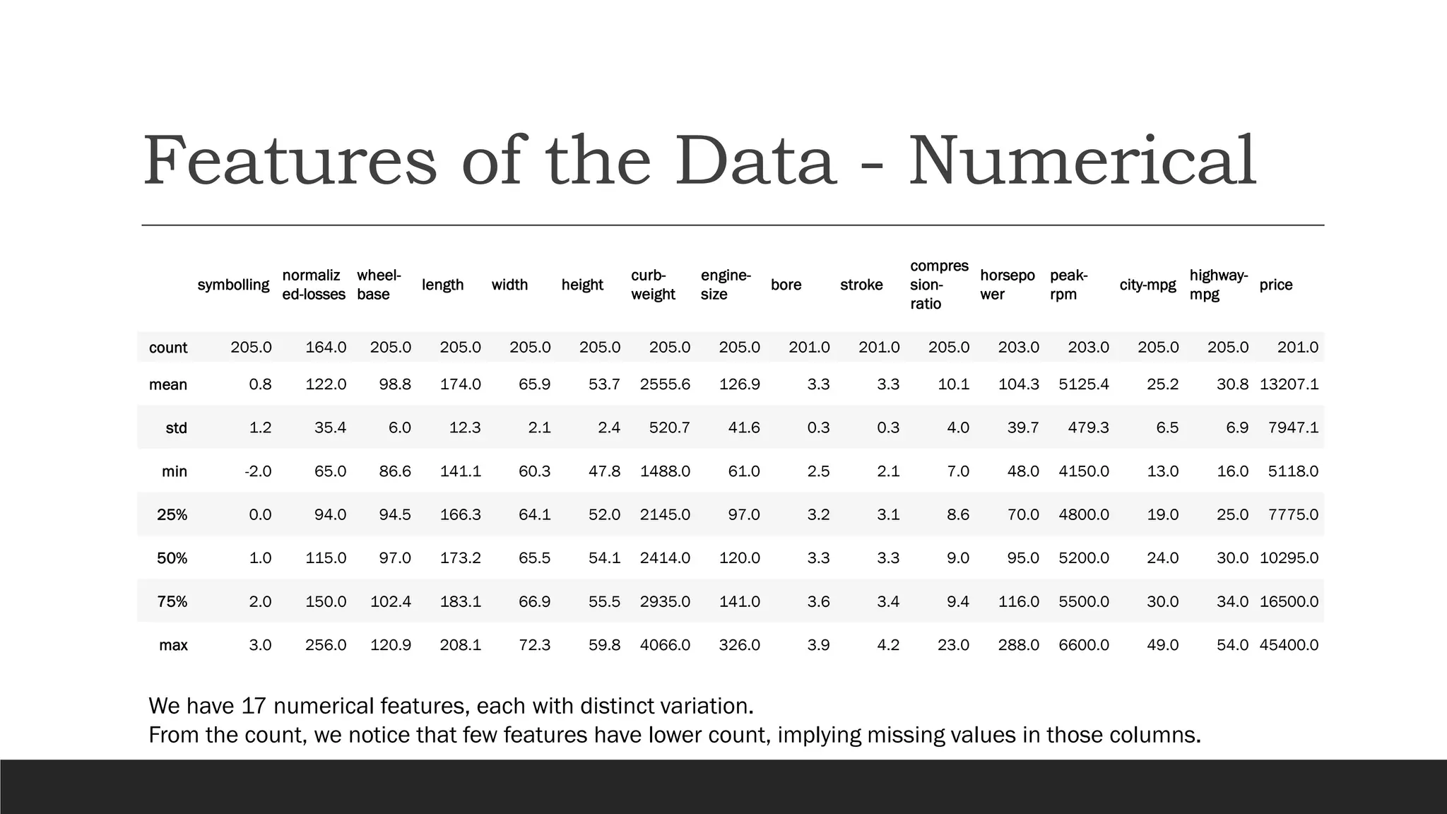
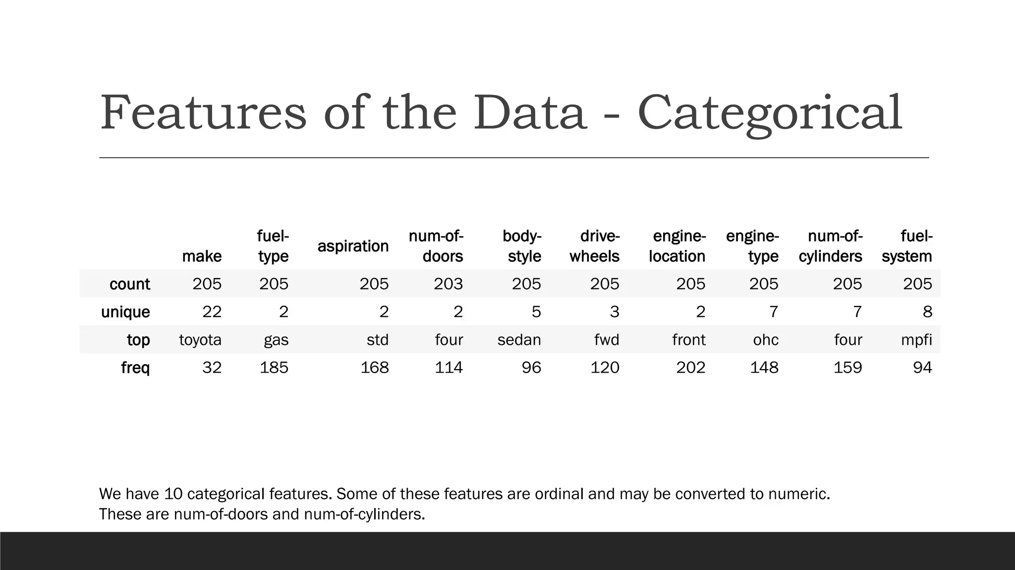
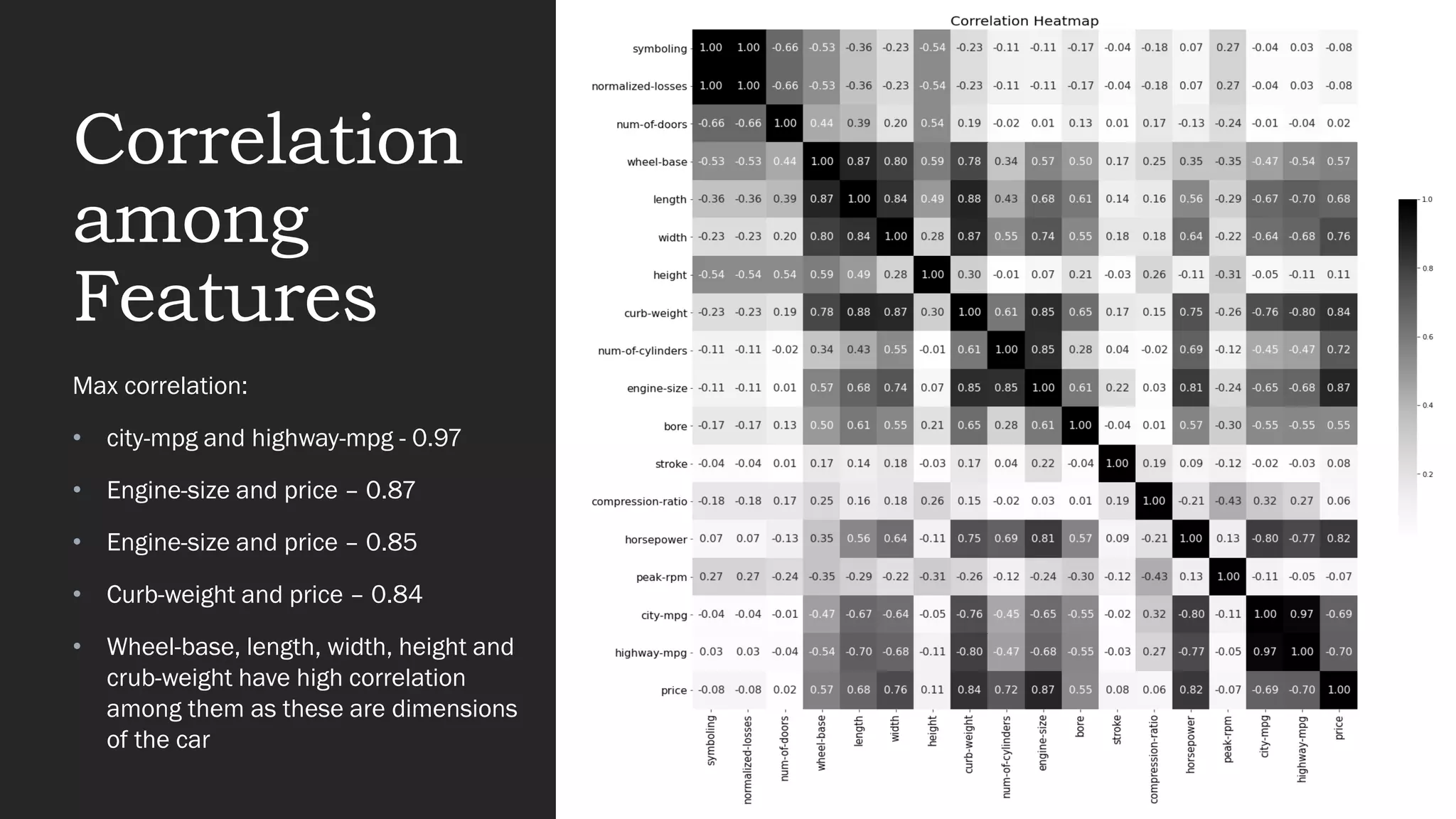
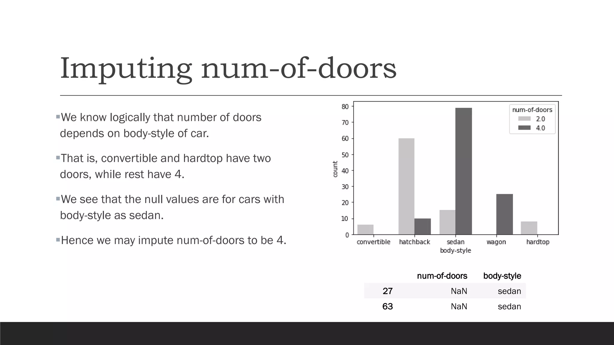
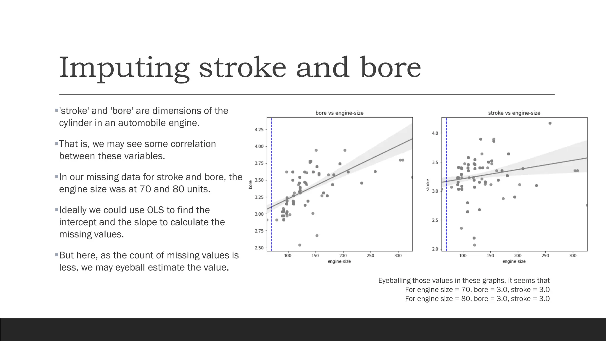
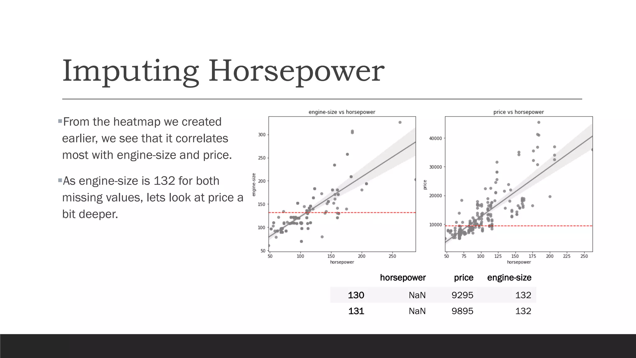
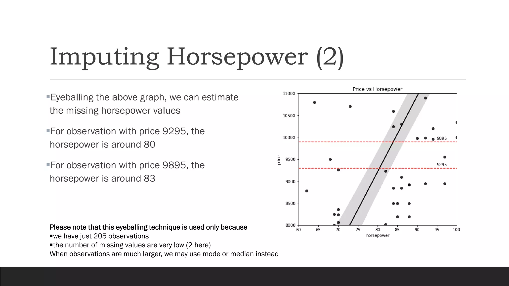
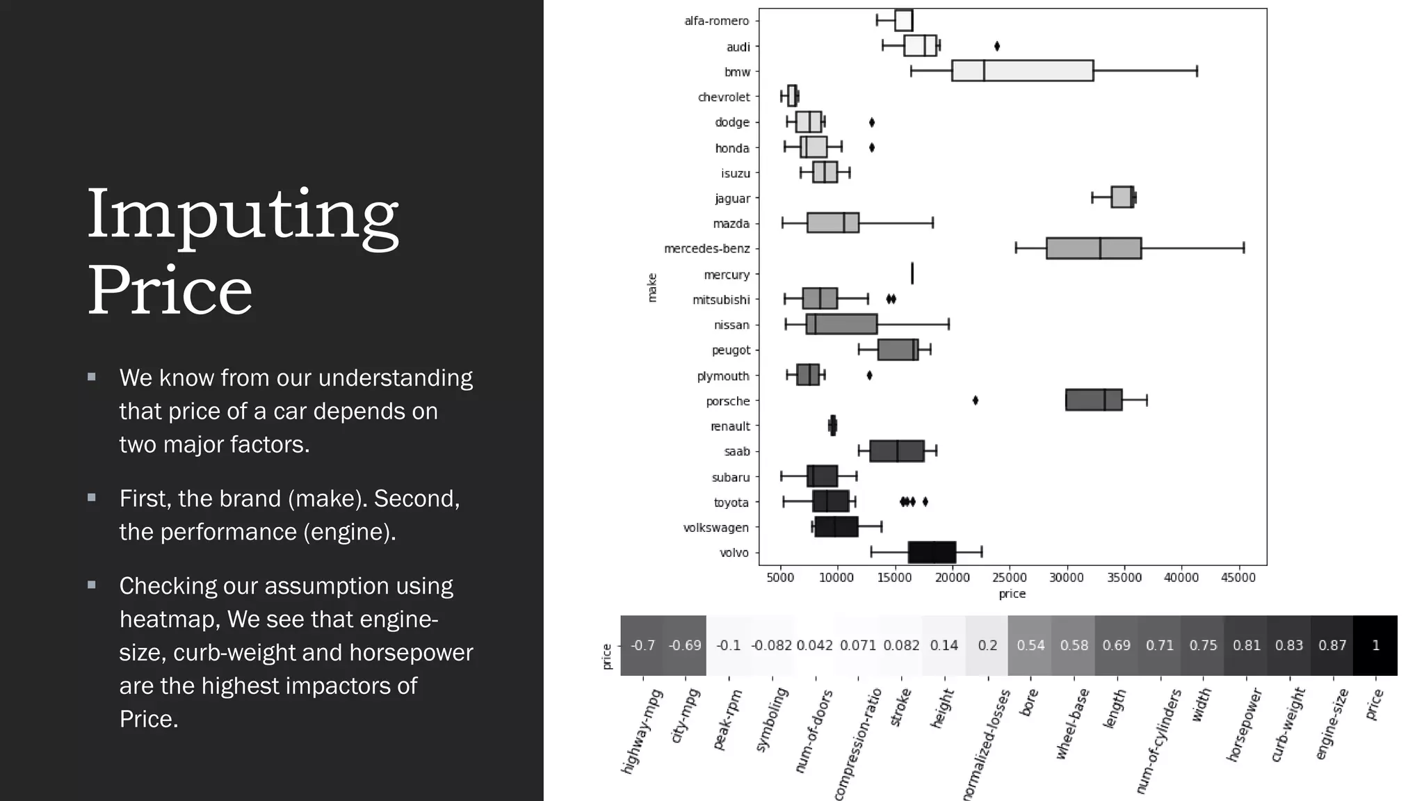
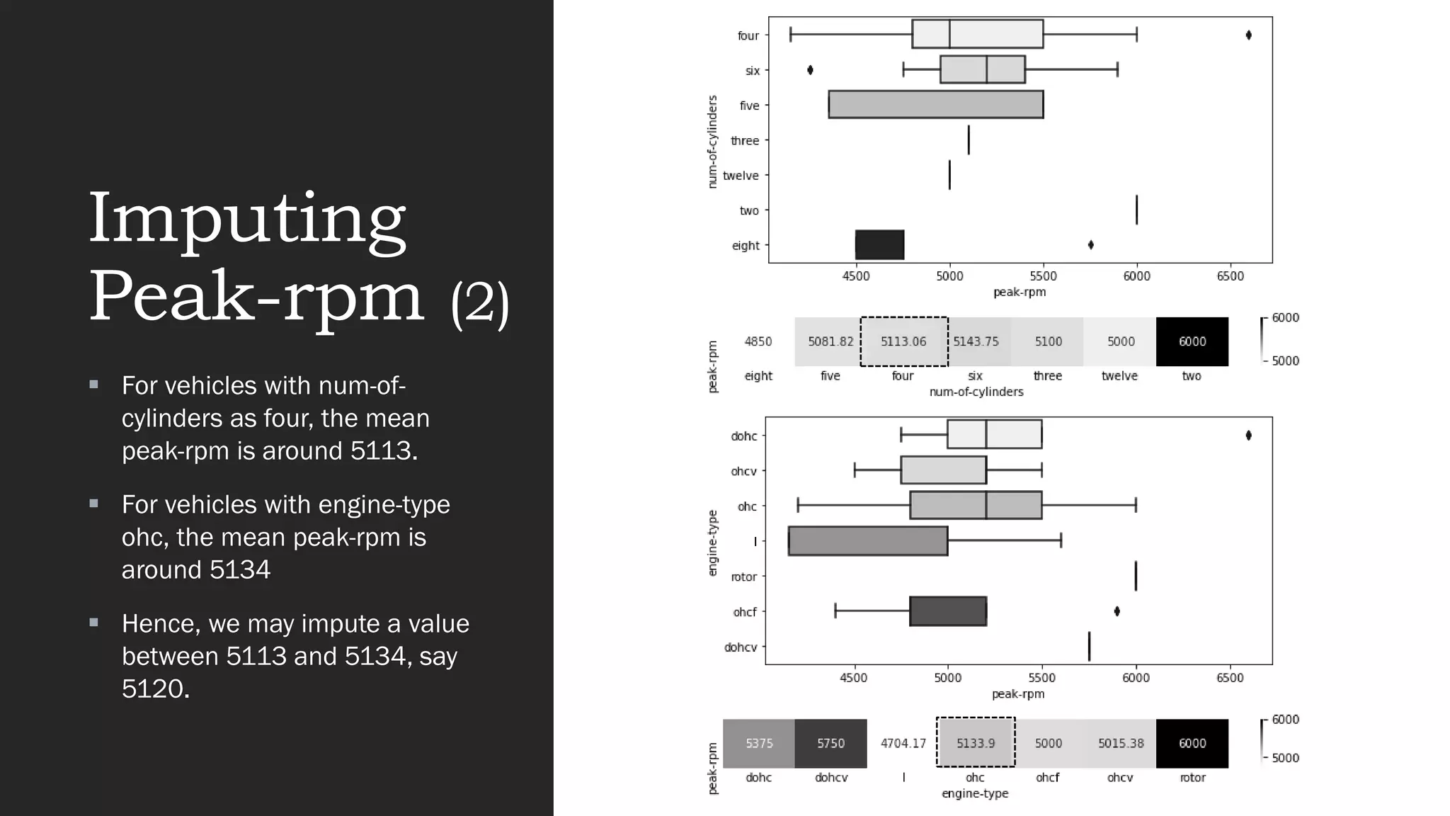
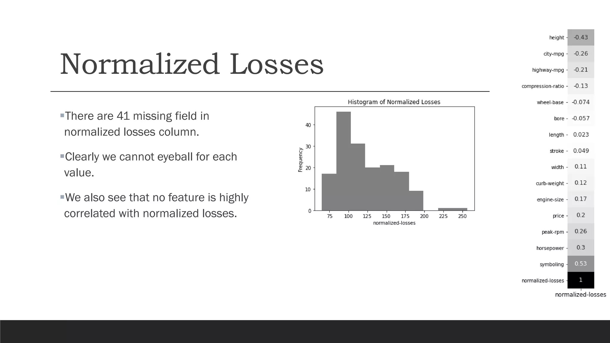
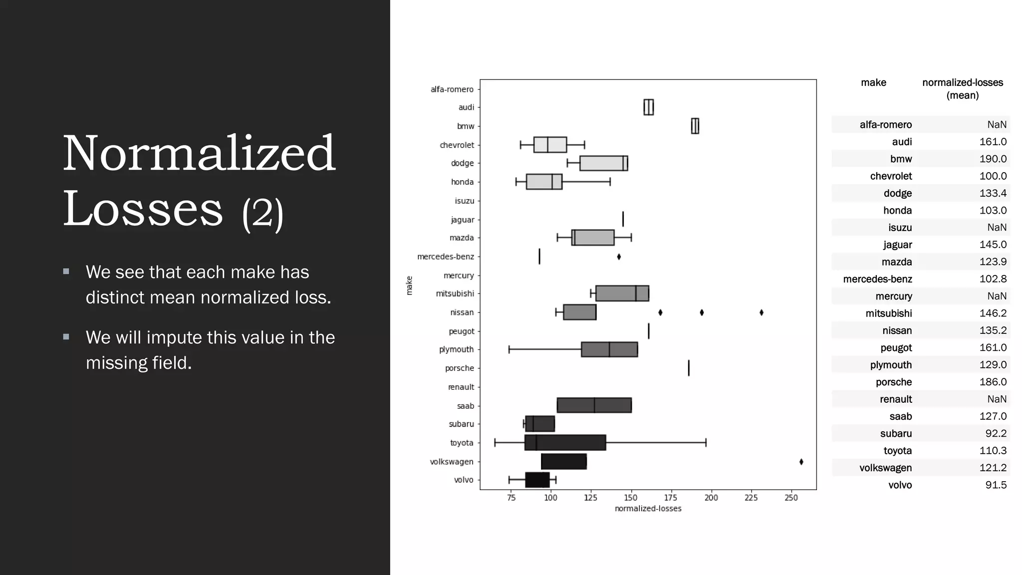
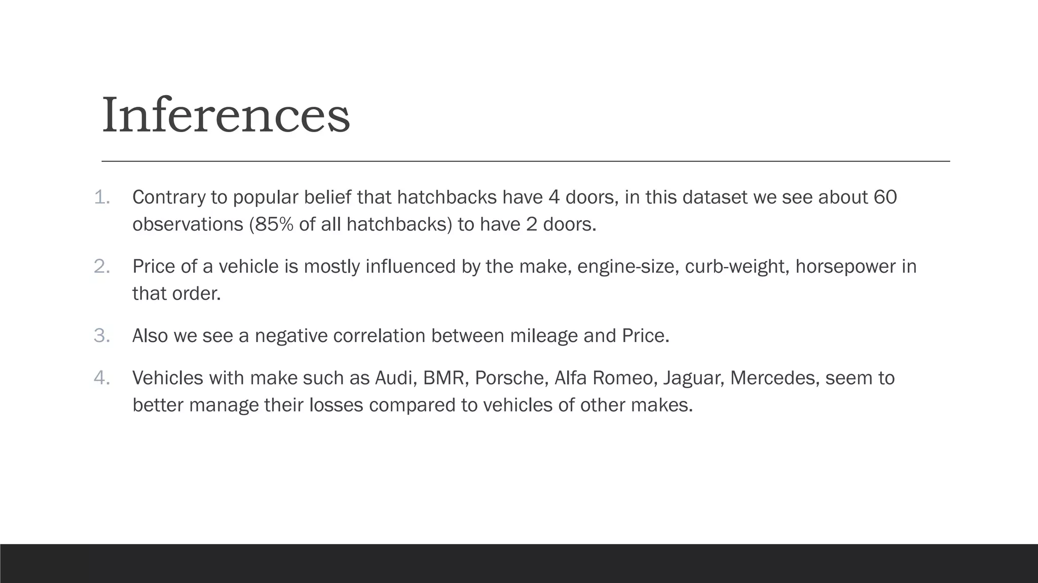
1. Automobile
Dataset
EDA
KENNY D
SEPT 2021

2. “In God we trust;
all others must bring data.”
- WILLIAM EDWARDS DEMMINGS
(STATISTICIAN, DATA SCIENTIST)

3. Contents
1. Introduction.......................................................................................04
2. Features of the Data
▪ Numerical……………………………………………………………………………………….05
▪ Categorical …………………………………………………………………………………….06
3. Correlation among Features ……………………………………………………….07
4. Missing Values imputation
▪ Number of Doors ……………………………………………………………………………09
▪ Stroke and Bore ………………………………………………………………………..10
▪ Horsepower ……………………………………………………………………………………11
▪ Price ……………………………………………………………………………………….13
▪ Peak-rpm …………………………………………………………………………………16
▪ Normalized Loses ……………………………………………………………………..18
5. Conclusion …..………………………………………………………………………..20
6. Inference ……….……………………………………………………………………………21

4. Introduction
We are presented with a small automobile dataset with just 205 observations.
Each observation constitutes of 26 features of automobiles such as make, horsepower, price and
more.
In this report, we will strive to draw relationships between each feature and present useful
inferences.

5. Features of the Data - Numerical
symbolling
normaliz
ed-losses
wheel-
base
length width height
curb-
weight
engine-
size
bore stroke
compres
sion-
ratio
horsepo
wer
peak-
rpm
city-mpg
highway-
mpg
price
count 205.0 164.0 205.0 205.0 205.0 205.0 205.0 205.0 201.0 201.0 205.0 203.0 203.0 205.0 205.0 201.0
mean 0.8 122.0 98.8 174.0 65.9 53.7 2555.6 126.9 3.3 3.3 10.1 104.3 5125.4 25.2 30.8 13207.1
std 1.2 35.4 6.0 12.3 2.1 2.4 520.7 41.6 0.3 0.3 4.0 39.7 479.3 6.5 6.9 7947.1
min -2.0 65.0 86.6 141.1 60.3 47.8 1488.0 61.0 2.5 2.1 7.0 48.0 4150.0 13.0 16.0 5118.0
25% 0.0 94.0 94.5 166.3 64.1 52.0 2145.0 97.0 3.2 3.1 8.6 70.0 4800.0 19.0 25.0 7775.0
50% 1.0 115.0 97.0 173.2 65.5 54.1 2414.0 120.0 3.3 3.3 9.0 95.0 5200.0 24.0 30.0 10295.0
75% 2.0 150.0 102.4 183.1 66.9 55.5 2935.0 141.0 3.6 3.4 9.4 116.0 5500.0 30.0 34.0 16500.0
max 3.0 256.0 120.9 208.1 72.3 59.8 4066.0 326.0 3.9 4.2 23.0 288.0 6600.0 49.0 54.0 45400.0
We have 17 numerical features, each with distinct variation.
From the count, we notice that few features have lower count, implying missing values in those columns.

6. Features of the Data - Categorical
make
fuel-
type
aspiration
num-of-
doors
body-
style
drive-
wheels
engine-
location
engine-
type
num-of-
cylinders
fuel-
system
count 205 205 205 203 205 205 205 205 205 205
unique 22 2 2 2 5 3 2 7 7 8
top toyota gas std four sedan fwd front ohc four mpfi
freq 32 185 168 114 96 120 202 148 159 94
We have 10 categorical features. Some of these features are ordinal and may be converted to numeric.
These are num-of-doors and num-of-cylinders.

7. Correlation
among
Features
Max correlation:
• city-mpg and highway-mpg - 0.97
• Engine-size and price – 0.87
• Engine-size and price – 0.85
• Curb-weight and price – 0.84
• Wheel-base, length, width, height and
crub-weight have high correlation
among them as these are dimensions
of the car

8. Missing values
Imputation
IN THE SUBSEQUENT SLIDES WE WILL IMPUTE THE MISSING
VALUES BASED ON INSIGHTS FROM EDA

9. Imputing num-of-doors
▪We know logically that number of doors
depends on body-style of car.
▪That is, convertible and hardtop have two
doors, while rest have 4.
▪We see that the null values are for cars with
body-style as sedan.
▪Hence we may impute num-of-doors to be 4.
num-of-doors body-style
27 NaN sedan
63 NaN sedan

10. Imputing stroke and bore
▪'stroke' and 'bore' are dimensions of the
cylinder in an automobile engine.
▪That is, we may see some correlation
between these variables.
▪In our missing data for stroke and bore, the
engine size was at 70 and 80 units.
▪Ideally we could use OLS to find the
intercept and the slope to calculate the
missing values.
▪But here, as the count of missing values is
less, we may eyeball estimate the value.
Eyeballing those values in these graphs, it seems that
For engine size = 70, bore = 3.0, stroke = 3.0
For engine size = 80, bore = 3.0, stroke = 3.0

11. Imputing Horsepower
▪From the heatmap we created
earlier, we see that it correlates
most with engine-size and price.
▪As engine-size is 132 for both
missing values, lets look at price a
bit deeper.
horsepower price engine-size
130 NaN 9295 132
131 NaN 9895 132

12. Imputing Horsepower (2)
▪Eyeballing the above graph, we can estimate
the missing horsepower values
▪For observation with price 9295, the
horsepower is around 80
▪For observation with price 9895, the
horsepower is around 83
Please note that this eyeballing technique is used only because
▪we have just 205 observations
▪the number of missing values are very low (2 here)
When observations are much larger, we may use mode or median instead

13. Imputing
Price
▪ We know from our understanding
that price of a car depends on
two major factors.
▪ First, the brand (make). Second,
the performance (engine).
▪ Checking our assumption using
heatmap, We see that engine-
size, curb-weight and horsepower
are the highest impactors of
Price.

14. Imputing Price (2)
▪In line with our assumption, Price is
dependent on engine-size, horsepower
and the make of the vehicle.
▪Lets look at this deeper.
make horsepower price engine-size
9 audi 160.0 NaN 131
44 isuzu 70.0 NaN 90
45 isuzu 70.0 NaN 90
129 porsche 288.0 NaN 203

15. Imputing Price (3)
From above we can estimate,
▪for an Audi with engine-size 131, the price can be around 22000
▪for an isuzu with engine-size 90, the price can be around 7000
▪for a porsche with engine-size 203, the price can be around 37500

16. Imputing
Peak-rpm
▪ We see that there are no
features that are highly
correlated with peak-rpm.
▪ Hence we look at categorical
features instead.
▪ As engine-type and num-of-
cylinders have 7 unique
variations, we will use that to
impute value for peak-rpm.
130 131 count unique top freq
make renault renault 205 22 toyota 32
fuel-type gas gas 205 2 gas 185
aspiration std std 205 2 std 168
num-of-
doors
four two 205 3 four 114
body-style wagon hatchback 205 5 sedan 96
drive-
wheels
fwd fwd 205 3 fwd 120
engine-
location
front front 205 2 front 202
engine-
type
ohc ohc 205 7 ohc 148
num-of-
cylinders
four four 205 7 four 159
fuel-
system
mpfi mpfi 205 8 mpfi 94
peak-rpm NaN NaN - - - -

17. Imputing
Peak-rpm (2)
▪ For vehicles with num-of-
cylinders as four, the mean
peak-rpm is around 5113.
▪ For vehicles with engine-type
ohc, the mean peak-rpm is
around 5134
▪ Hence, we may impute a value
between 5113 and 5134, say
5120.

18. Normalized Losses
▪There are 41 missing field in
normalized losses column.
▪Clearly we cannot eyeball for each
value.
▪We also see that no feature is highly
correlated with normalized losses.

19. Normalized
Losses (2)
▪ We see that each make has
distinct mean normalized loss.
▪ We will impute this value in the
missing field.
make normalized-losses
(mean)
alfa-romero NaN
audi 161.0
bmw 190.0
chevrolet 100.0
dodge 133.4
honda 103.0
isuzu NaN
jaguar 145.0
mazda 123.9
mercedes-benz 102.8
mercury NaN
mitsubishi 146.2
nissan 135.2
peugot 161.0
plymouth 129.0
porsche 186.0
renault NaN
saab 127.0
subaru 92.2
toyota 110.3
volkswagen 121.2
volvo 91.5

20. Conclusion
▪In this project, we have analysed the data between
multiple features of automobiles to establish each’s
relationship with the other and impute the missing fields
within the dataset.
▪We have successfully imputed all missing values with
appropriate metrics.
▪While doing so, we have uncovered several insights from
the data which we present in the subsequent slide.

21. Inferences
1. Contrary to popular belief that hatchbacks have 4 doors, in this dataset we see about 60
observations (85% of all hatchbacks) to have 2 doors.
2. Price of a vehicle is mostly influenced by the make, engine-size, curb-weight, horsepower in
that order.
3. Also we see a negative correlation between mileage and Price.
4. Vehicles with make such as Audi, BMR, Porsche, Alfa Romeo, Jaguar, Mercedes, seem to
better manage their losses compared to vehicles of other makes.