FBS-Group-A06-Project-Report.pdf

The automobile data analysis includes a dataset introduced from the Univerisity of California Irvine
Machine Learning Repository UCI. According to UCI (1985), the attributes consist of three different
types of entities: (a) the model and specification of an auto, which includes the characteristics, (b) the
personal insurance, (c) its normalized losses in use as compared to other cars. The data set source for
this model collected from Insurance collision reports, personal insurance, and car models. There are
26 data attributes in this model descript the data set model from different angles. The objective of this
report is to perform exploratory data analysis to find the primary relationships between features,
which include univariate analysis, which includes finding the maximum and minimum, such as the
weight, engine size, horsepower, and price. Moreover, perform a regression to predict the car prices.
AUTOMOBILE DATA ANALYSIS
Sri Mounica Kalidasu,Anand Desika, Saketh GV, Praveen Kumar A, Marcel Tino
EXPLORATORY ANALYSIS
Importing Libraries and Setting up Input Path
In [1]: #Importing Libraries
import numpy as np
import pandas as pd
import seaborn as sns
import matplotlib.pyplot as plt
# Input data files from specified paths
import warnings
warnings.filterwarnings("ignore")
import os
print(os.listdir("C:/Users/kalid/Downloads/input"))
#Input Excel File
df_automobile = pd.read_csv("C:/Users/kalid/Downloads/input/Automobile_da
ta.csv")
Data Cleaning
Data contains "?" replace it with NAN
['Automobile_data.csv']

In [2]: df_data = df_automobile.replace('?',np.NAN)
df_data.isnull().sum()
Finding Range of each Attribute present in the
Dataset
Out[2]: symboling 0
normalized-losses 41
make 0
fuel-type 0
aspiration 0
num-of-doors 2
body-style 0
drive-wheels 0
engine-location 0
wheel-base 0
length 0
width 0
height 0
curb-weight 0
engine-type 0
num-of-cylinders 0
engine-size 0
fuel-system 0
bore 4
stroke 4
compression-ratio 0
horsepower 2
peak-rpm 2
city-mpg 0
highway-mpg 0
price 4
dtype: int64

In [3]: for col in df_automobile:
col_vals = df_automobile[col].unique()
print (col,":tt",sorted(col_vals))
print('n')

symboling : [-2, -1, 0, 1, 2, 3]
normalized-losses : ['101', '102', '103', '104', '106', '10
7', '108', '110', '113', '115', '118', '119', '121', '122', '125', '128',
'129', '134', '137', '142', '145', '148', '150', '153', '154', '158', '16
1', '164', '168', '186', '188', '192', '194', '197', '231', '256', '65',
'74', '77', '78', '81', '83', '85', '87', '89', '90', '91', '93', '94',
'95', '98', '?']
make : ['alfa-romero', 'audi', 'bmw', 'chevrolet', 'dodge', 'ho
nda', 'isuzu', 'jaguar', 'mazda', 'mercedes-benz', 'mercury', 'mitsubish
i', 'nissan', 'peugot', 'plymouth', 'porsche', 'renault', 'saab', 'subar
u', 'toyota', 'volkswagen', 'volvo']
fuel-type : ['diesel', 'gas']
aspiration : ['std', 'turbo']
num-of-doors : ['?', 'four', 'two']
body-style : ['convertible', 'hardtop', 'hatchback', 'sedan',
'wagon']
drive-wheels : ['4wd', 'fwd', 'rwd']
engine-location : ['front', 'rear']
wheel-base : [86.6, 88.4, 88.6, 89.5, 91.3, 93.0, 93.1, 93.3,
93.7, 94.3, 94.5, 95.1, 95.3, 95.7, 95.9, 96.0, 96.1, 96.3, 96.5, 96.6, 9
6.9, 97.0, 97.2, 97.3, 98.4, 98.8, 99.1, 99.2, 99.4, 99.5, 99.8, 100.4, 1
01.2, 102.0, 102.4, 102.7, 102.9, 103.3, 103.5, 104.3, 104.5, 104.9, 105.
8, 106.7, 107.9, 108.0, 109.1, 110.0, 112.0, 113.0, 114.2, 115.6, 120.9]
length : [141.1, 144.6, 150.0, 155.9, 156.9, 157.1, 157.
3, 157.9, 158.7, 158.8, 159.1, 159.3, 162.4, 163.4, 165.3, 165.6, 165.7,
166.3, 166.8, 167.3, 167.5, 168.7, 168.8, 168.9, 169.0, 169.1, 169.7, 17
0.2, 170.7, 171.2, 171.7, 172.0, 172.4, 172.6, 173.0, 173.2, 173.4, 173.
5, 173.6, 174.6, 175.0, 175.4, 175.6, 175.7, 176.2, 176.6, 176.8, 177.3,
177.8, 178.2, 178.4, 178.5, 180.2, 180.3, 181.5, 181.7, 183.1, 183.5, 18
4.6, 186.6, 186.7, 187.5, 187.8, 188.8, 189.0, 190.9, 191.7, 192.7, 193.
8, 197.0, 198.9, 199.2, 199.6, 202.6, 208.1]
width : [60.3, 61.8, 62.5, 63.4, 63.6, 63.8, 63.9, 64.0,
64.1, 64.2, 64.4, 64.6, 64.8, 65.0, 65.2, 65.4, 65.5, 65.6, 65.7, 66.0, 6
6.1, 66.2, 66.3, 66.4, 66.5, 66.6, 66.9, 67.2, 67.7, 67.9, 68.0, 68.3, 6
8.4, 68.8, 68.9, 69.6, 70.3, 70.5, 70.6, 70.9, 71.4, 71.7, 72.0, 72.3]

height : [47.8, 48.8, 49.4, 49.6, 49.7, 50.2, 50.5, 50.6,
50.8, 51.0, 51.4, 51.6, 52.0, 52.4, 52.5, 52.6, 52.8, 53.0, 53.1, 53.2, 5
3.3, 53.5, 53.7, 53.9, 54.1, 54.3, 54.4, 54.5, 54.7, 54.8, 54.9, 55.1, 5
5.2, 55.4, 55.5, 55.6, 55.7, 55.9, 56.0, 56.1, 56.2, 56.3, 56.5, 56.7, 5
7.5, 58.3, 58.7, 59.1, 59.8]
curb-weight : [1488, 1713, 1819, 1837, 1874, 1876, 1889, 1890,
1900, 1905, 1909, 1918, 1938, 1940, 1944, 1945, 1950, 1951, 1956, 1967, 1
971, 1985, 1989, 2004, 2008, 2010, 2015, 2017, 2024, 2028, 2037, 2040, 20
50, 2081, 2094, 2109, 2120, 2122, 2128, 2140, 2145, 2169, 2190, 2191, 220
4, 2209, 2212, 2221, 2236, 2240, 2254, 2261, 2264, 2265, 2275, 2280, 228
9, 2290, 2293, 2300, 2302, 2304, 2319, 2324, 2326, 2328, 2337, 2340, 236
5, 2370, 2372, 2380, 2385, 2395, 2403, 2405, 2410, 2414, 2420, 2425, 244
3, 2455, 2458, 2460, 2465, 2480, 2500, 2507, 2510, 2535, 2536, 2540, 254
8, 2551, 2563, 2579, 2650, 2658, 2661, 2670, 2679, 2695, 2700, 2707, 271
0, 2714, 2734, 2756, 2758, 2765, 2778, 2800, 2808, 2811, 2818, 2823, 282
4, 2833, 2844, 2847, 2910, 2912, 2921, 2926, 2935, 2952, 2954, 2975, 297
6, 3012, 3016, 3020, 3034, 3042, 3045, 3049, 3053, 3055, 3060, 3062, 307
1, 3075, 3086, 3095, 3110, 3130, 3131, 3139, 3151, 3157, 3197, 3217, 323
0, 3252, 3285, 3296, 3366, 3380, 3430, 3485, 3495, 3505, 3515, 3685, 371
5, 3740, 3750, 3770, 3900, 3950, 4066]
engine-type : ['dohc', 'dohcv', 'l', 'ohc', 'ohcf', 'ohcv', 'r
otor']
num-of-cylinders : ['eight', 'five', 'four', 'six', 'thre
e', 'twelve', 'two']
engine-size : [61, 70, 79, 80, 90, 91, 92, 97, 98, 103, 108, 1
09, 110, 111, 119, 120, 121, 122, 130, 131, 132, 134, 136, 140, 141, 145,
146, 151, 152, 156, 161, 164, 171, 173, 181, 183, 194, 203, 209, 234, 25
8, 304, 308, 326]
fuel-system : ['1bbl', '2bbl', '4bbl', 'idi', 'mfi', 'mpfi',
'spdi', 'spfi']
bore : ['2.54', '2.68', '2.91', '2.92', '2.97', '2.99', '3.01',
'3.03', '3.05', '3.08', '3.13', '3.15', '3.17', '3.19', '3.24', '3.27',
'3.31', '3.33', '3.34', '3.35', '3.39', '3.43', '3.46', '3.47', '3.5',
'3.54', '3.58', '3.59', '3.6', '3.61', '3.62', '3.63', '3.7', '3.74', '3.
76', '3.78', '3.8', '3.94', '?']
stroke : ['2.07', '2.19', '2.36', '2.64', '2.68', '2.76',
'2.8', '2.87', '2.9', '3.03', '3.07', '3.08', '3.1', '3.11', '3.12', '3.1
5', '3.16', '3.19', '3.21', '3.23', '3.27', '3.29', '3.35', '3.39', '3.
4', '3.41', '3.46', '3.47', '3.5', '3.52', '3.54', '3.58', '3.64', '3.8
6', '3.9', '4.17', '?']

Clean Missing Data
compression-ratio : [7.0, 7.5, 7.6, 7.7, 7.8, 8.0, 8.1, 8.3,
8.4, 8.5, 8.6, 8.7, 8.8, 9.0, 9.1, 9.2, 9.3, 9.31, 9.4, 9.41, 9.5, 9.6, 1
0.0, 10.1, 11.5, 21.0, 21.5, 21.9, 22.0, 22.5, 22.7, 23.0]
horsepower : ['100', '101', '102', '106', '110', '111', '11
2', '114', '115', '116', '120', '121', '123', '134', '135', '140', '142',
'143', '145', '152', '154', '155', '156', '160', '161', '162', '175', '17
6', '182', '184', '200', '207', '262', '288', '48', '52', '55', '56', '5
8', '60', '62', '64', '68', '69', '70', '72', '73', '76', '78', '82', '8
4', '85', '86', '88', '90', '92', '94', '95', '97', '?']
peak-rpm : ['4150', '4200', '4250', '4350', '4400', '4500',
'4650', '4750', '4800', '4900', '5000', '5100', '5200', '5250', '5300',
'5400', '5500', '5600', '5750', '5800', '5900', '6000', '6600', '?']
city-mpg : [13, 14, 15, 16, 17, 18, 19, 20, 21, 22, 23, 24,
25, 26, 27, 28, 29, 30, 31, 32, 33, 34, 35, 36, 37, 38, 45, 47, 49]
highway-mpg : [16, 17, 18, 19, 20, 22, 23, 24, 25, 26, 27, 28,
29, 30, 31, 32, 33, 34, 36, 37, 38, 39, 41, 42, 43, 46, 47, 50, 53, 54]
price : ['10198', '10245', '10295', '10345', '10595', '1
0698', '10795', '10898', '10945', '11048', '11199', '11245', '11248', '11
259', '11549', '11595', '11694', '11845', '11850', '11900', '12170', '122
90', '12440', '12629', '12764', '12940', '12945', '12964', '13200', '1329
5', '13415', '13495', '13499', '13645', '13845', '13860', '13950', '1439
9', '14489', '14869', '15040', '15250', '15510', '15580', '15645', '1569
0', '15750', '15985', '15998', '16430', '16500', '16503', '16515', '1655
8', '16630', '16695', '16845', '16900', '16925', '17075', '17199', '1745
0', '17669', '17710', '17950', '18150', '18280', '18344', '18399', '1842
0', '18620', '18920', '18950', '19045', '19699', '20970', '21105', '2148
5', '22018', '22470', '22625', '23875', '24565', '25552', '28176', '2824
8', '30760', '31600', '32250', '32528', '34028', '34184', '35056', '3555
0', '36000', '36880', '37028', '40960', '41315', '45400', '5118', '5151',
'5195', '5348', '5389', '5399', '5499', '5572', '6095', '6189', '6229',
'6295', '6338', '6377', '6479', '6488', '6529', '6575', '6649', '6669',
'6692', '6695', '6785', '6795', '6849', '6855', '6918', '6938', '6989',
'7053', '7099', '7126', '7129', '7198', '7295', '7299', '7349', '7395',
'7463', '7499', '7603', '7609', '7689', '7738', '7775', '7788', '7799',
'7895', '7898', '7957', '7975', '7995', '7999', '8013', '8058', '8189',
'8195', '8238', '8249', '8358', '8449', '8495', '8499', '8558', '8778',
'8845', '8921', '8948', '8949', '9095', '9233', '9258', '9279', '9295',
'9298', '9495', '9538', '9549', '9639', '9895', '9959', '9960', '9980',
'9988', '9989', '9995', '?']

Fill missing data of normalised-losses, price, horsepower, peak-rpm, bore, stroke with the
respective column mean
Fill missing data category Number of doors with the mode of the column

In [4]: df_temp = df_automobile[df_automobile[' normalized-losses']!='?']
normalised_mean = df_temp[' normalized-losses'].astype(int).mean()
df_automobile[' normalized-losses'] = df_automobile[' normalized-losses']
.replace('?',normalised_mean).astype(int)
df_temp = df_automobile[df_automobile[' price']!='?']
normalised_mean = df_temp[' price'].astype(int).mean()
df_automobile[' price'] = df_automobile[' price'].replace('?',normalised_
mean).astype(int)
df_temp = df_automobile[df_automobile[' horsepower']!='?']
normalised_mean = df_temp[' horsepower'].astype(int).mean()
df_automobile[' horsepower'] = df_automobile[' horsepower'].replace('?',n
ormalised_mean).astype(int)
df_temp = df_automobile[df_automobile[' peak-rpm']!='?']
normalised_mean = df_temp[' peak-rpm'].astype(int).mean()
df_automobile[' peak-rpm'] = df_automobile[' peak-rpm'].replace('?',norma
lised_mean).astype(int)
df_temp = df_automobile[df_automobile[' bore']!='?']
normalised_mean = df_temp[' bore'].astype(float).mean()
df_automobile[' bore'] = df_automobile[' bore'].replace('?',normalised_me
an).astype(float)
df_temp = df_automobile[df_automobile[' stroke']!='?']
normalised_mean = df_temp[' stroke'].astype(float).mean()
df_automobile[' stroke'] = df_automobile[' stroke'].replace('?',normalise
d_mean).astype(float)
df_automobile[' num-of-doors'] = df_automobile[' num-of-doors'].replace(
'?','four')
df_automobile.head()
Summary statistics of variable
Out[4]:
symboling
normalized-
losses
make
fuel-
type
aspiration
num-
of-
doors
body-
style
drive-
wheels
eng
locat
0 3 122
alfa-
romero
gas std two convertible rwd f
1 3 122
alfa-
romero
2 1 122
alfa-
romero
gas std two hatchback rwd f
3 2 164 audi gas std four sedan fwd f
4 2 164 audi gas std four sedan 4wd f
5 rows × 26 columns

In [5]: df_automobile.describe()
Visualising numerical data
Out[5]:
symboling
normalized-
losses
wheel-
base
length width height c
count 205.000000 205.000000 205.000000 205.000000 205.000000 205.000000
mean 0.834146 122.000000 98.756585 174.049268 65.907805 53.724878 2
std 1.245307 31.681008 6.021776 12.337289 2.145204 2.443522
min -2.000000 65.000000 86.600000 141.100000 60.300000 47.800000 1
25% 0.000000 101.000000 94.500000 166.300000 64.100000 52.000000 2
50% 1.000000 122.000000 97.000000 173.200000 65.500000 54.100000 2
75% 2.000000 137.000000 102.400000 183.100000 66.900000 55.500000 2
max 3.000000 256.000000 120.900000 208.100000 72.300000 59.800000 4

In [6]: def scatter(x,fig):
plt.subplot(5,2,fig)
plt.scatter(df_automobile[x],df_automobile[' price'])
plt.title(x+' vs Price')
plt.ylabel('Price')
plt.xlabel(x)
plt.figure(figsize=(10,20))
scatter(' length', 1)
scatter(' width', 2)
scatter(' height', 3)
scatter(' curb-weight', 4)
plt.tight_layout()
Findings
width, length and curbweight seems to have a poitive correlation with price.
height does not show any signiﬁcant trend with price.
Univariate Analysis

In [7]: # 1 plt.figure(figsize=(10,8))
df_automobile[[' engine-size',' peak-rpm',' curb-weight',' compression-ra
tio',' horsepower',' price']].hist(figsize=(10,8),bins=6,color='Y')
# 2 plt.figure(figsize=(10,8))
plt.tight_layout()
plt.show()
Findings
Compression Ratio of the cars is in a range of 5 to 13
Most of the car has a Curb Weight is in range 1900 to 3100
The Engine Size is inrange 60 to 190
Most vehicle has horsepower 50 to 125
Most Vehicle are in price range 5000 to 18000
peak rpm is mostly distributed between 4600 to 5700

In [8]: plt.figure(1)
plt.subplot(221)
df_automobile[' engine-type'].value_counts(normalize=True).plot(figsize=(
10,8),kind='bar',color='red')
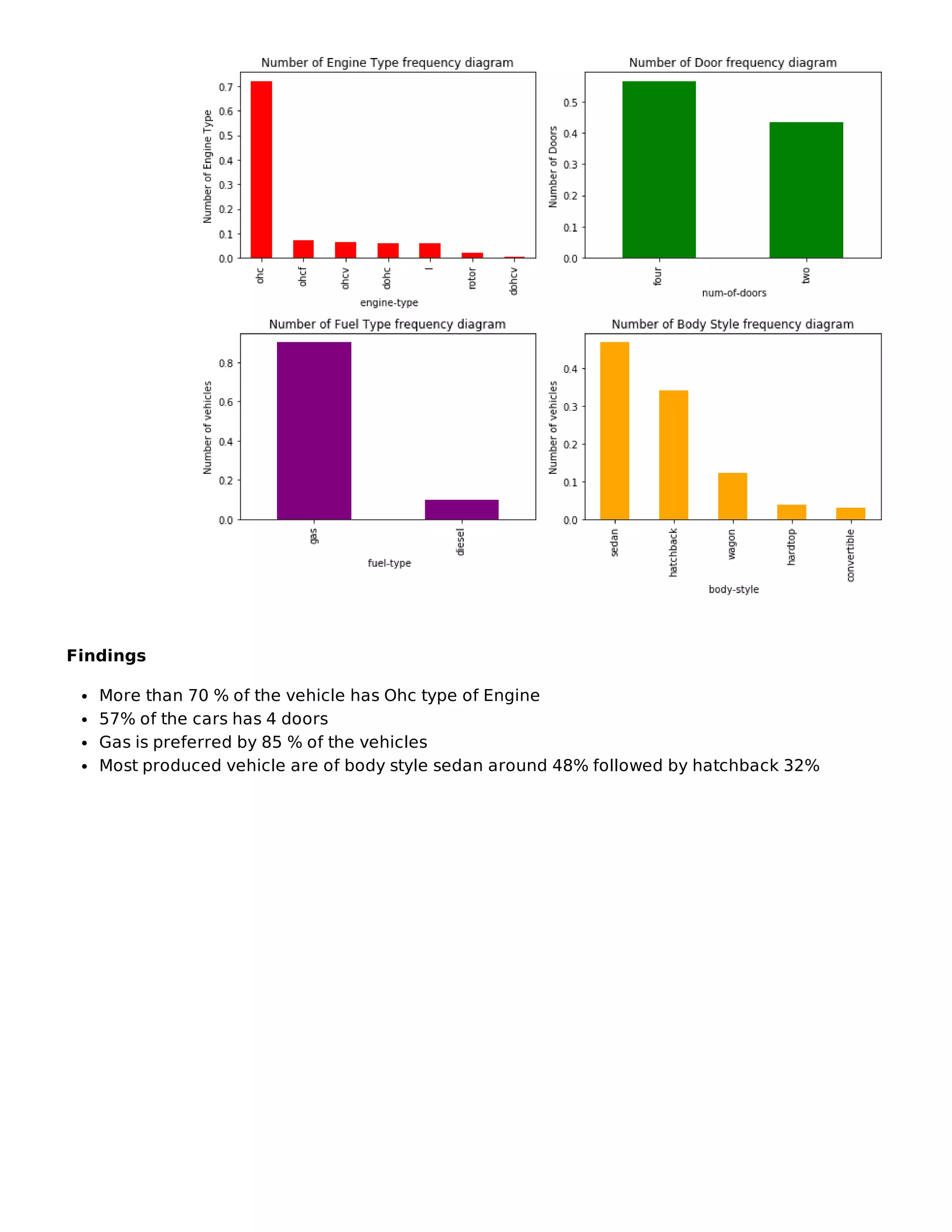
plt.title("Number of Engine Type frequency diagram")
plt.ylabel('Number of Engine Type')
plt.xlabel(' engine-type');
plt.subplot(222)
df_automobile[' num-of-doors'].value_counts(normalize=True).plot(figsize=
(10,8),kind='bar',color='green')
plt.title("Number of Door frequency diagram")
plt.ylabel('Number of Doors')
plt.xlabel(' num-of-doors');
plt.subplot(223)
df_automobile[' fuel-type'].value_counts(normalize= True).plot(figsize=(1
0,8),kind='bar',color='purple')
plt.title("Number of Fuel Type frequency diagram")
plt.ylabel('Number of vehicles')
plt.xlabel(' fuel-type');
plt.subplot(224)
df_automobile[' body-style'].value_counts(normalize=True).plot(figsize=(1
0,8),kind='bar',color='orange')
plt.title("Number of Body Style frequency diagram")
plt.ylabel('Number of vehicles')
plt.xlabel(' body-style');
plt.tight_layout()
plt.show()

Findings
More than 70 % of the vehicle has Ohc type of Engine
57% of the cars has 4 doors
Gas is preferred by 85 % of the vehicles
Most produced vehicle are of body style sedan around 48% followed by hatchback 32%

In [9]: import seaborn as sns
corr = df_automobile.corr()
plt.figure(figsize=(20,9))
a = sns.heatmap(corr, annot=True, fmt='.2f')
Findings
curb-size, engine-size, horsepower are positively corelated
city-mpg,highway-mpg are negatively corelate
Bivariate Analysis (PRICE ANALYSIS)

In [10]: plt.figure(figsize=(25, 6))
df = pd.DataFrame(df_automobile.groupby([' make'])[' price'].mean().sort_
values(ascending = False))
df.plot.bar()
plt.title('Company Name vs Average Price')
plt.show()
df = pd.DataFrame(df_automobile.groupby([' fuel-type'])[' price'].mean().
sort_values(ascending = False))
df.plot.bar()
plt.title('Fuel Type vs Average Price')
plt.show()
df = pd.DataFrame(df_automobile.groupby([' body-style'])[' price'].mean()
.sort_values(ascending = False))
df.plot.bar()
plt.title(' body-style vs Average Price')
plt.show()

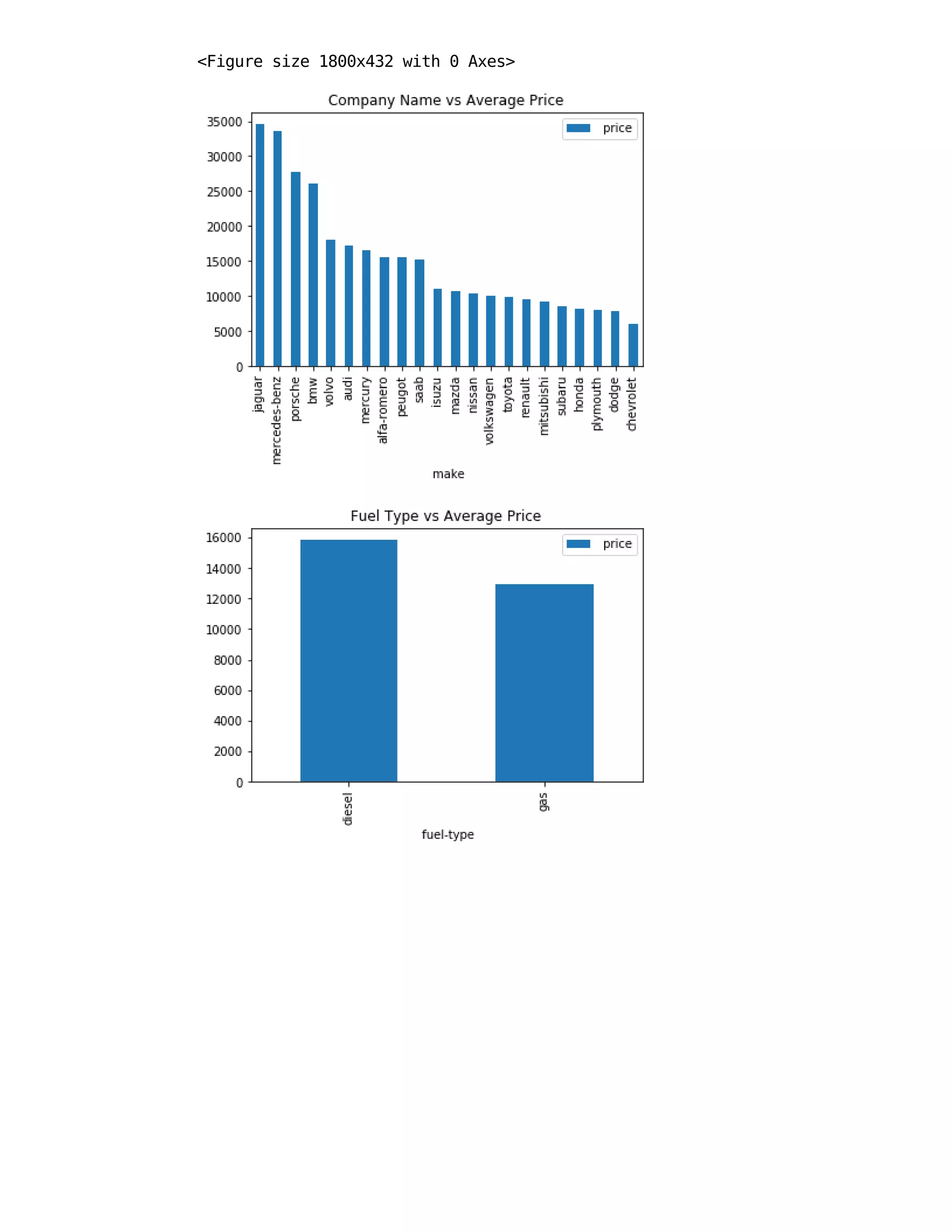
Findings
Jaguar and Buick seem to have highest average price.
diesel has higher average price than gas.
hardtop and convertible have higher average price.
In [11]: plt.rcParams['figure.figsize']=(20,6)
ax = sns.boxplot(x=" make", y=" price", data=df_automobile)

In [12]: sns.catplot(data=df_automobile, x=" body-style", y=" price", hue=" aspira
tion" ,kind="point")
ax = sns.boxplot(x=" drive-wheels", y=" price", data=df_automobile)
Out[12]: <seaborn.axisgrid.FacetGrid at 0x24a1c094a88>

Findings
Mercedez-Benz ,BMW, Jaguar, Porshe produces expensive cars more than 25000
cheverolet,dodge, honda,mitbushi, nissan,plymouth subaru,toyata produces budget models
with lower prices
most of the cars comapany produces car in range below 25000
Hardtop model are expensive in prices followed by convertible and sedan body style
Turbo models have higher prices than for the standard model
Convertible has only standard edition with expensive cars
hatchback and sedan turbo models are available below 20000
rwd wheel drive vehicle have expensive prices
ax = sns.boxenplot(x=" engine-type", y=" price", data=df_automobile)
ay = sns.swarmplot(x=" engine-type", y=" engine-size", data=df_automobil
e)

In [16]: sns.catplot(data=df_automobile, x=" num-of-cylinders", y=" horsepower")
Findings
ohc is the most used Engine Type both for diesel and gas
Diesel vehicle have Engine type "ohc" and "I" and engine size ranges between 100 to 190
Engine type ohcv has the bigger Engine size ranging from 155 to 300
Body-style Hatchback uses max variety of Engine Type followed by sedan
Body-style Convertible is not available with Diesel Engine type
Vehicle with above 200 horsepower has Eight Twelve Six cyclinders
Out[16]: <seaborn.axisgrid.FacetGrid at 0x24a1bf3e148>

In [17]: sns.catplot(data=df_automobile, y=" normalized-losses", x=" symboling" ,
hue=" body-style" ,kind="point")
Losses Findings
Note :- here +3 means risky vehicle and -2 means safe vehicle
Increased in risk rating linearly increases in normalised losses in vehicle
covertible car and hardtop car has mostly losses with risk rating above 0
hatchback cars has highest losses at risk rating 3
sedan and Wagon car has losses even in less risk (safe)rating
Out[17]: <seaborn.axisgrid.FacetGrid at 0x24a1bf84908>

In [18]: g = sns.pairplot(df_automobile[[" city-mpg", " horsepower", " engine-siz
e", " curb-weight"," price", " fuel-type"]], hue=" fuel-type", diag_kind=
"hist")
Findings
Vehicle Mileage decrease as increase in Horsepower , engine-size, Curb Weight
As horsepower increase the engine size increases
Curbweight increases with the increase in Engine Size
Price Analysis
engine size and curb-weight is positively co realted with price
city-mpg is negatively corelated with price as increase horsepower reduces the mileage
Deriving new features

Fuel economy and Cars Range
In [19]: df_automobile[' fueleconomy'] = (0.55 * df_automobile[' city-mpg']) + (0.
45 * df_automobile[' highway-mpg'])
In [20]: #Binning the Car Companies based on avg prices of each Company.
df_automobile[' price'] = df_automobile[' price'].astype('int')
temp = df_automobile.copy()
table = temp.groupby([' make'])[' price'].mean()
temp = temp.merge(table.reset_index(), how='left',on=' make')
bins = [0,10000,20000,40000]
cars_bin=['Budget','Medium','Highend']
df_automobile['carsrange'] = pd.cut(temp[' price_y'],bins,right=False,lab
els=cars_bin)
df_automobile.head()
Out[20]:
symboling
normalized-
losses
make
fuel-
type
aspiration
num-
of-
doors
body-
style
drive-
wheels
eng
locat
0 3 122
alfa-
romero
1 3 122
alfa-
romero
2 1 122
alfa-
romero
gas std two hatchback rwd f
3 2 164 audi gas std four sedan fwd f
4 2 164 audi gas std four sedan 4wd f

In [21]: plt.figure(figsize=(25, 6))
df = pd.DataFrame(df_automobile.groupby([' fuel-system',' drive-wheels',
'carsrange'])[' price'].mean().unstack(fill_value=0))
df.plot.bar()
plt.title('Car Range vs Average Price')
plt.show()
In [22]: df_automobile_lr = df_automobile[[' price', ' fuel-type', ' aspiration','
body-style',' drive-wheels',' wheel-base',
' curb-weight', ' engine-type', ' num-of-cylinders', '
engine-size', ' bore',' horsepower',' fueleconomy',
' height', ' length',' width', 'carsrange']]
df_automobile_lr.head()
<Figure size 1800x432 with 0 Axes>
Out[22]:
price
fuel-
type
aspiration
body-
style
drive-
wheels
wheel-
base
curb-
weight
engine-
type
num-of-
cylinders
e
0 13495 gas std convertible rwd 88.6 2548 dohc four
1 16500 gas std convertible rwd 88.6 2548 dohc four
2 16500 gas std hatchback rwd 94.5 2823 ohcv six
3 13950 gas std sedan fwd 99.8 2337 ohc four
4 17450 gas std sedan 4wd 99.4 2824 ohc ﬁve

In [23]: sns.pairplot(df_automobile_lr)
plt.show()
Correlations between all numeric values from the new dataframe deﬁned
Fueleconomy is negatively correlated with all the variables
PREDICTIVE ANALYSIS
Dummy Variables

In [24]: # Defining the map function
def dummies(x,df):
temp = pd.get_dummies(df[x], drop_first = True)
df = pd.concat([df, temp], axis = 1)
df.drop([x], axis = 1, inplace = True)
return df
# Applying the function to the cars_lr
df_automobile_lr = dummies(' fuel-type',df_automobile_lr)
df_automobile_lr = dummies(' aspiration',df_automobile_lr)
df_automobile_lr = dummies(' body-style',df_automobile_lr)
df_automobile_lr = dummies(' drive-wheels',df_automobile_lr)
df_automobile_lr = dummies(' engine-type',df_automobile_lr)
df_automobile_lr = dummies(' num-of-cylinders',df_automobile_lr)
df_automobile_lr = dummies('carsrange',df_automobile_lr)
In [25]: df_automobile_lr.head()
In [26]: df_automobile_lr.shape
Train-Test Split and feature scaling
Out[25]:
price
wheel-
base
curb-
weight
engine-
size
bore horsepower fueleconomy height length
0 13495 88.6 2548 130 3.47 111 23.70 48.8 168.8
1 16500 88.6 2548 130 3.47 111 23.70 48.8 168.8
2 16500 94.5 2823 152 2.68 154 22.15 52.4 171.2
3 13950 99.8 2337 109 3.19 102 26.70 54.3 176.6
4 17450 99.4 2824 136 3.19 115 19.80 54.3 176.6
Out[26]: (205, 32)

In [27]: from sklearn.model_selection import train_test_split
np.random.seed(0)
df_train, df_test = train_test_split(df_automobile_lr, train_size = 0.7,
test_size = 0.3, random_state = 100)
from sklearn.preprocessing import MinMaxScaler
scaler = MinMaxScaler()
num_vars = [' wheel-base', ' curb-weight', ' engine-size', ' bore', ' hor
sepower',' fueleconomy',' length',' width',' price']
df_train[num_vars] = scaler.fit_transform(df_train[num_vars])
df_train.head()
In [28]: df_train.describe()
Out[27]:
price
wheel-
base
curb-
weight
engine-
size
bore horsepower fueleconomy h
122 0.068818 0.244828 0.272692 0.139623 0.230159 0.083333 0.530864
125 0.466890 0.272414 0.500388 0.339623 1.000000 0.395833 0.213992
166 0.122110 0.272414 0.314973 0.139623 0.444444 0.266667 0.344307
1 0.314446 0.068966 0.411171 0.260377 0.626984 0.262500 0.244170
199 0.382131 0.610345 0.647401 0.260377 0.746032 0.475000 0.122085
Out[28]:
price
wheel-
base
curb-
weight
engine-
size
bore horsepower fu
count 143.000000 143.000000 143.000000 143.000000 143.000000 143.000000
mean 0.216554 0.411141 0.407878 0.241351 0.497941 0.228118
std 0.210700 0.205581 0.211269 0.154619 0.207140 0.165395
min 0.000000 0.000000 0.000000 0.000000 0.000000 0.000000
25% 0.067298 0.272414 0.245539 0.135849 0.305556 0.091667
50% 0.144404 0.341379 0.355702 0.184906 0.500000 0.195833
75% 0.300398 0.503448 0.559542 0.301887 0.682540 0.283333
max 1.000000 1.000000 1.000000 1.000000 1.000000 1.000000

In [29]: #Correlation using heatmap
plt.figure(figsize = (30, 25))
sns.heatmap(df_train.corr(), annot = True, cmap="YlGnBu")
plt.show()
Highly correlated variables to price are - curbweight , enginesize , horsepower , carwidth
and highend .
In [30]: #Dividing data into X and y variables
y_train = df_train.pop(' price')
X_train = df_train
Model Building
Recursive Feature Elimination (RFE) is popular because it is easy to conﬁgure and use and
because it is eﬀective at selecting those features (columns) in a training dataset that are more
or most relevant in predicting the target variable.

In [31]: #RFE
from sklearn.feature_selection import RFE
from sklearn.linear_model import LinearRegression
import statsmodels.api as sm
from statsmodels.stats.outliers_influence import variance_inflation_facto
r
lm = LinearRegression()
lm.fit(X_train,y_train)
rfe = RFE(lm, 10)
rfe = rfe.fit(X_train, y_train)
list(zip(X_train.columns,rfe.support_,rfe.ranking_))
In [32]: X_train.columns[rfe.support_]
Building model using statsmodel, for the detailed
statistics
Out[31]: [(' wheel-base', False, 2),
(' curb-weight', True, 1),
(' engine-size', False, 13),
(' bore', False, 11),
(' horsepower', True, 1),
(' fueleconomy', True, 1),
(' height', False, 22),
(' length', False, 5),
(' width', True, 1),
('gas', False, 17),
('turbo', False, 18),
('hardtop', False, 3),
('hatchback', True, 1),
('sedan', True, 1),
('wagon', True, 1),
('fwd', False, 21),
('rwd', False, 15),
('dohcv', True, 1),
('l', False, 16),
('ohc', False, 8),
('ohcf', False, 9),
('ohcv', False, 12),
('rotor', False, 19),
('five', False, 6),
('four', False, 4),
('six', False, 7),
('three', False, 14),
('twelve', True, 1),
('two', False, 20),
('Medium', False, 10),
('Highend', True, 1)]
Out[32]: Index([' curb-weight', ' horsepower', ' fueleconomy', ' width', 'hatchbac
k',
'sedan', 'wagon', 'dohcv', 'twelve', 'Highend'],
dtype='object')

In [33]: X_train_rfe = X_train[X_train.columns[rfe.support_]]
X_train_rfe.head()
In [34]: def build_model(X,y):
X = sm.add_constant(X) #Adding the constant
lm = sm.OLS(y,X).fit() # fitting the model
print(lm.summary()) # model summary
return X
def checkVIF(X):
vif = pd.DataFrame()
vif['Features'] = X.columns
vif['VIF'] = [variance_inflation_factor(X.values, i) for i in range(X
.shape[1])]
vif['VIF'] = round(vif['VIF'], 2)
vif = vif.sort_values(by = "VIF", ascending = False)
return(vif)
There are some guidelines we can use to determine whether our VIFs are in an acceptable
range. A rule of thumb commonly used in practice is if a VIF is > 10, you have high
multicollinearity.
MODEL1
Out[33]:
curb-
weight
horsepower fueleconomy width hatchback sedan wagon doh
122 0.272692 0.083333 0.530864 0.291667 0 1 0
125 0.500388 0.395833 0.213992 0.666667 1 0 0
166 0.314973 0.266667 0.344307 0.308333 1 0 0
1 0.411171 0.262500 0.244170 0.316667 0 0 0
199 0.647401 0.475000 0.122085 0.575000 0 0 1

In [35]: X_train_new = build_model(X_train_rfe,y_train)

OLS Regression Results
=========================================================================
=====
Dep. Variable: price R-squared:
0.914
Model: OLS Adj. R-squared:
0.908
Method: Least Squares F-statistic:
140.6
Date: Thu, 04 Mar 2021 Prob (F-statistic): 2.6
9e-65
Time: 22:08:06 Log-Likelihood: 1
95.85
No. Observations: 143 AIC: -
369.7
Df Residuals: 132 BIC: -
337.1
Df Model: 10
Covariance Type: nonrobust
=========================================================================
=======
coef std err t P>|t| [0.025
0.975]
-------------------------------------------------------------------------
-------
const -0.1011 0.045 -2.232 0.027 -0.191
-0.012
curb-weight 0.2623 0.073 3.575 0.000 0.117
0.407
horsepower 0.4583 0.079 5.792 0.000 0.302
0.615
fueleconomy 0.1200 0.056 2.146 0.034 0.009
0.231
width 0.2539 0.066 3.832 0.000 0.123
0.385
hatchback -0.0984 0.027 -3.660 0.000 -0.152
-0.045
sedan -0.0675 0.027 -2.533 0.012 -0.120
-0.015
wagon -0.1002 0.030 -3.346 0.001 -0.159
-0.041
dohcv -0.7665 0.084 -9.076 0.000 -0.934
-0.599
twelve -0.1179 0.072 -1.631 0.105 -0.261
0.025
Highend 0.2626 0.021 12.243 0.000 0.220
0.305
=========================================================================
=====
Omnibus: 36.397 Durbin-Watson:
1.842
Prob(Omnibus): 0.000 Jarque-Bera (JB): 8
1.418
Skew: 1.064 Prob(JB): 2.0
9e-18
Kurtosis: 6.022 Cond. No.
31.8

p-vale of twelve seems to be higher than the signiﬁcance value of 0.05, hence dropping it as
it is insigniﬁcant in presence of other variables.
In [36]: X_train_new = X_train_rfe.drop(["twelve"], axis = 1)
MODEL2
=========================================================================
=====
Warnings:
[1] Standard Errors assume that the covariance matrix of the errors is co
rrectly specified.

In [37]: X_train_new = build_model(X_train_new,y_train)

=========================================================================
=====
0.912
0.907
154.0
9e-66
94.42
368.8
339.2
Df Model: 9
=========================================================================
=======
0.975]
-------------------------------------------------------------------------
-------
const -0.0830 0.044 -1.878 0.063 -0.170
0.004
curb-weight 0.2716 0.074 3.691 0.000 0.126
0.417
horsepower 0.4086 0.073 5.560 0.000 0.263
0.554
fueleconomy 0.1004 0.055 1.826 0.070 -0.008
0.209
width 0.2516 0.067 3.774 0.000 0.120
0.383
hatchback -0.1005 0.027 -3.719 0.000 -0.154
-0.047
sedan -0.0715 0.027 -2.678 0.008 -0.124
-0.019
wagon -0.1052 0.030 -3.512 0.001 -0.165
-0.046
dohcv -0.7313 0.082 -8.901 0.000 -0.894
-0.569
Highend 0.2605 0.022 12.091 0.000 0.218
0.303
=========================================================================
=====
1.864
0.963
9e-22
29.4
=========================================================================
=====

In [39]: X_train_new = X_train_new.drop([" fueleconomy"], axis = 1)
MODEL 3
Warnings:
rrectly specified.

=========================================================================
=====
0.910
0.905
169.9
8e-66
92.65
367.3
340.6
Df Model: 8
=========================================================================
=======
0.975]
-------------------------------------------------------------------------
-------
const -0.0205 0.028 -0.727 0.469 -0.076
0.035
curb-weight 0.2490 0.073 3.402 0.001 0.104
0.394
horsepower 0.3364 0.062 5.384 0.000 0.213
0.460
width 0.2398 0.067 3.583 0.000 0.107
0.372
hatchback -0.0965 0.027 -3.554 0.001 -0.150
-0.043
sedan -0.0670 0.027 -2.500 0.014 -0.120
-0.014
wagon -0.1047 0.030 -3.464 0.001 -0.164
-0.045
dohcv -0.6838 0.079 -8.699 0.000 -0.839
-0.528
Highend 0.2667 0.021 12.429 0.000 0.224
0.309
=========================================================================
=====
1.906
0.780
0e-25
27.0
=========================================================================
=====
Warnings:

In [41]: #Calculating the Variance Inflation Factor
checkVIF(X_train_new)
dropping curbweight because of high VIF value. (shows that curbweight has high
multicollinearity.)
In [43]: X_train_new = X_train_new.drop([" curb-weight"], axis = 1)
MODEL 4
rrectly specified.
Out[41]:
Features VIF
0 const 26.88
1 curb-weight 8.04
5 sedan 6.08
4 hatchback 5.63
3 width 5.13
2 horsepower 3.59
6 wagon 3.56
8 Highend 1.63
7 dohcv 1.45

=========================================================================
=====
0.902
0.897
178.5
9e-65
86.73
357.5
333.7
Df Model: 7
=========================================================================
======
0.975]
-------------------------------------------------------------------------
------
const -0.0216 0.029 -0.739 0.461 -0.079
0.036
horsepower 0.4528 0.054 8.339 0.000 0.345
0.560
width 0.4107 0.046 8.950 0.000 0.320
0.501
hatchback -0.1085 0.028 -3.877 0.000 -0.164
-0.053
sedan -0.0714 0.028 -2.568 0.011 -0.126
-0.016
wagon -0.0876 0.031 -2.830 0.005 -0.149
-0.026
dohcv -0.7924 0.075 -10.624 0.000 -0.940
-0.645
Highend 0.2824 0.022 12.977 0.000 0.239
0.325
=========================================================================
=====
2.009
0.944
5e-18
18.0
=========================================================================
=====
Warnings:
rrectly specified.

In [45]: checkVIF(X_train_new)
dropping sedan because of high VIF value.
In [46]: X_train_new = X_train_new.drop(["sedan"], axis = 1)
MODEL 5
Out[45]:
Features VIF
0 const 26.88
4 sedan 6.06
3 hatchback 5.54
5 wagon 3.47
1 horsepower 2.52
2 width 2.24
7 Highend 1.56
6 dohcv 1.21

=========================================================================
=====
0.898
0.893
199.0
2e-65
83.32
352.6
331.9
Df Model: 6
=========================================================================
======
0.975]
-------------------------------------------------------------------------
------
const -0.0797 0.019 -4.205 0.000 -0.117
-0.042
horsepower 0.4825 0.054 8.913 0.000 0.375
0.590
width 0.3816 0.045 8.411 0.000 0.292
0.471
hatchback -0.0451 0.013 -3.349 0.001 -0.072
-0.018
wagon -0.0221 0.018 -1.234 0.219 -0.057
0.013
dohcv -0.8017 0.076 -10.546 0.000 -0.952
-0.651
Highend 0.2858 0.022 12.895 0.000 0.242
0.330
=========================================================================
=====
2.021
6.745
7e-11
16.4
=========================================================================
=====
Warnings:
rrectly specified.

dropping wagon because of high p-value.
In [49]: X_train_new = X_train_new.drop(["wagon"], axis = 1)
MODEL 6
Out[48]:
Features VIF
0 const 10.83
1 horsepower 2.40
2 width 2.10
6 Highend 1.55
3 hatchback 1.23
5 dohcv 1.21
4 wagon 1.11

=========================================================================
=====
0.897
0.893
237.5
8e-65
82.52
353.0
335.3
Df Model: 5
=========================================================================
======
0.975]
-------------------------------------------------------------------------
------
const -0.0843 0.019 -4.533 0.000 -0.121
-0.048
horsepower 0.4835 0.054 8.916 0.000 0.376
0.591
width 0.3805 0.045 8.371 0.000 0.291
0.470
hatchback -0.0403 0.013 -3.119 0.002 -0.066
-0.015
dohcv -0.8050 0.076 -10.577 0.000 -0.956
-0.655
Highend 0.2891 0.022 13.117 0.000 0.246
0.333
=========================================================================
=====
2.029
3.141
9e-12
16.3
=========================================================================
=====
Warnings:
rrectly specified.

MODEL 7
Out[51]:
Features VIF
0 const 10.40
1 horsepower 2.40
2 width 2.10
5 Highend 1.53
4 dohcv 1.21
3 hatchback 1.13

In [52]: #Dropping dohcv to see the changes in model statistics
X_train_new = X_train_new.drop(["dohcv"], axis = 1)
X_train_new = build_model(X_train_new,y_train)
checkVIF(X_train_new)

=========================================================================
=====
0.812
0.807
149.1
0e-49
39.84
269.7
254.9
Df Model: 4
=========================================================================
======
0.975]
-------------------------------------------------------------------------
------
const -0.0482 0.025 -1.964 0.052 -0.097
0.000
horsepower 0.3310 0.070 4.715 0.000 0.192
0.470
width 0.3822 0.061 6.263 0.000 0.262
0.503
hatchback -0.0595 0.017 -3.466 0.001 -0.093
-0.026
Highend 0.2793 0.030 9.444 0.000 0.221
0.338
=========================================================================
=====
1.913
9.928
Skew: -2.007 Prob(JB):
0.00
13.0
=========================================================================
=====
Warnings:
rrectly specified.

Residual Analysis of Model
In [53]: lm = sm.OLS(y_train,X_train_new).fit()
y_train_price = lm.predict(X_train_new)
In [54]: # Plot the histogram of the error terms
fig = plt.figure()
sns.distplot((y_train - y_train_price), bins = 20)
fig.suptitle('Error Terms', fontsize = 20) # Plot headin
g
plt.xlabel('Errors', fontsize = 18)
Error terms seem to be approximately normally distributed, so the assumption on the linear
modeling seems to be fulﬁlled.
Prediction and Evaluation
In [56]: #Scaling the test set
num_vars = [' wheel-base', ' curb-weight', ' engine-size', ' bore', ' hor
sepower',' fueleconomy',' length',' width',' price']
df_test[num_vars] = scaler.fit_transform(df_test[num_vars])
Out[52]:
Features VIF
0 const 10.05
1 horsepower 2.23
2 width 2.10
4 Highend 1.53
3 hatchback 1.11
Out[54]: Text(0.5, 0, 'Errors')

In [57]: #Dividing into X and y
y_test = df_test.pop(' price')
X_test = df_test
In [58]: # Now let's use our model to make predictions.
X_train_new = X_train_new.drop('const',axis=1)
# Creating X_test_new dataframe by dropping variables from X_test
X_test_new = X_test[X_train_new.columns]
# Adding a constant variable
X_test_new = sm.add_constant(X_test_new)
In [59]: # Making predictions
y_pred = lm.predict(X_test_new)
Evaluation of test via comparison of y_pred and
y_test
In [60]: from sklearn.metrics import r2_score
r2_score(y_test, y_pred)
In [61]: #EVALUATION OF THE MODEL
# Plotting y_test and y_pred to understand the spread.
fig = plt.figure()
plt.scatter(y_test,y_pred)
fig.suptitle('y_test vs y_pred', fontsize=20) # Plot heading
plt.xlabel('y_test', fontsize=18) # X-label
plt.ylabel('y_pred', fontsize=16)
Evaluation of the model using Statistics
Out[60]: 0.9037424400203523
Out[61]: Text(0, 0.5, 'y_pred')

In [62]: print(lm.summary())
=========================================================================
=====
0.812
0.807
149.1
0e-49
39.84
269.7
254.9
Df Model: 4
=========================================================================
======
0.975]
-------------------------------------------------------------------------
------
const -0.0482 0.025 -1.964 0.052 -0.097
0.000
horsepower 0.3310 0.070 4.715 0.000 0.192
0.470
width 0.3822 0.061 6.263 0.000 0.262
0.503
hatchback -0.0595 0.017 -3.466 0.001 -0.093
-0.026
Highend 0.2793 0.030 9.444 0.000 0.221
0.338
=========================================================================
=====
1.913
9.928
Skew: -2.007 Prob(JB):
0.00
13.0
=========================================================================
=====
Warnings:
rrectly specified.

Findings
R-sqaured and Adjusted R-squared (extent of fit) - 0.899 and 0.896 - 90% variance explained.
F-stats and Prob(F-stats) (overall model fit) - 308.0 and 1.04e-67(approx. 0.0) - Model fir is
significant and explained 90% variance is just not by chance.
p-values - p-values for all the coefficients seem to be less than the significance level of 0.05. -
meaning that all the predictors are statistically significant.
In [64]: import sklearn.metrics as sm
print("Mean absolute error =", round(sm.mean_absolute_error(y_test, y_pre
d), 5))
#print("Root Mean Squared Error =", round(sm.sqrt(mean_squared_error(y_te
st, y_pred)),5))
print("Mean squared error =", round(sm.mean_squared_error(y_test, y_pred
), 5))
print("Median absolute error =", round(sm.median_absolute_error(y_test, y
_pred), 5))
print("Explain variance score =", round(sm.explained_variance_score(y_tes
t, y_pred), 5))
print("R2 score =", round(sm.r2_score(y_test, y_pred), 5))
Mean absolute error: This is the average of absolute errors of all the data points in the given
dataset.
Mean squared error: This is the average of the squares of the errors of all the data points in
the given dataset. It is one of the most popular metrics out there!
Median absolute error: This is the median of all the errors in the given dataset. The main
advantage of this metric is that it's robust to outliers. A single bad point in the test dataset
wouldn't skew the entire error metric, as opposed to a mean error metric.
Explained variance score: This score measures how well our model can account for the
variation in our dataset. A score of 1.0 indicates that our model is perfect.
R2 score: This is pronounced as R-squared, and this score refers to the coefficient of
determination. This tells us how well the unknown samples will be predicted by our model. The
best possible score is 1.0, but the score can be negative as well.
A good practice is to make sure that the mean squared error is low and the explained variance
score is high.
Mean absolute error = 0.05202
Mean squared error = 0.00421
Median absolute error = 0.04143
Explain variance score = 0.90954
R2 score = 0.90374

In [66]: from nbconvert import HTMLExporter
import codecs
import nbformat
notebook_name = 'A06_FBS_Assignment2.ipynb'
output_file_name = 'FBS-Group-A06-Project-Report.html'
exporter = HTMLExporter()
output_notebook = nbformat.read(notebook_name, as_version=4)
output, resources = exporter.from_notebook_node(output_notebook)
codecs.open(output_file_name, 'w', encoding='utf-8').write(output)
In [ ]:

FBS-Group-A06-Project-Report.pdf

Recommended

Recommended

More Related Content

Similar to FBS-Group-A06-Project-Report.pdf

Similar to FBS-Group-A06-Project-Report.pdf (6)

Recently uploaded

Recently uploaded (20)

FBS-Group-A06-Project-Report.pdf