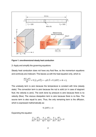
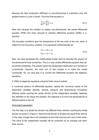
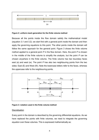
Chapter 3 focuses on steady diffusion problems, specifically heat and momentum diffusion, and introduces a five-step methodology for solving the governing partial differential equations. It details the process of converting these equations into algebraic forms using the finite volume method, particularly for one-dimensional steady heat conduction, including grid generation and numerical solution techniques. The chapter concludes with instructions for solving the resulting algebraic equations and reporting temperature distribution results.

1. 1
Chapter 3
Steady Diffusion problems
3.1. Introduction
After deriving the partial differential equations (PDEs) describing fluid flow and heat
transfer problems, we now need to establish the methodology used to solve these
PDEs. The first family of problems is steady diffusion. This chapter describes two
diffusion problems: heat diffusion and momentum diffusion. We will now apply the
five step approach introduced in the previous chapter to solve the governing
equations. These steps are:
1- Define a specific flow problem
2- Apply and simplify the governing equation
3- Convert the governing equations to algebraic equations using the finite
volume method
4- Solve the algebraic equations numerically
5- Report the results
3.2. One dimensional steady heat conduction
1- Problem description
One-dimensional steady heat conduction problems can occur in both solids and
fluids. Despite the governing equations used in this module describe fluid flow; they
can be used to model heat transfer in solids as well—via the temperature diffusion
term in the energy equation, because this term is the same for heat transfer in solids.
One-dimensional heat conduction implies that the temperature gradients are
negligible in the two other directions. If the material is fluid, the fluid velocity has to
be zero. Figure 1 shows some examples of one-dimensional steady heat conduction
problems.

2. 2
Figure 1: one-dimensional steady heat conduction
2- Apply and simplify the governing equations
Steady heat conduction does not have any fluid flow, so the momentum equations
and continuity are irrelevant. This leaves us with the heat equation only, which is:
( )
( ⃗
⃗ ) ⃗
⃗ ( )
The unsteady term is zero because the temperature is constant with time (steady
state). The convection term is zero because the rod is solid (or in case of stagnant
fluid, the velocity is zero). The work done by pressure is zero because there is no
velocity (flow). The viscous dissipation term is zero because there is no flow. The
source term is also equal to zero. Thus, the only remaining term is the diffusion,
which is expressed mathematically as:
( )
Expanding the equation
( ) ( ) ( )

3. 3
Because the heat conduction (diffusion) is one-dimensional in x-direction only, the
gradient terms in y and z vanish. Thus the final equation is:
( ) (3.1)
Note that because the problem is steady one-dimensional, the partial differential
equation (PDE) has been reduced to ordinary differential equation (ODE) in x-
direction.
The boundary conditions give the temperature at the two ends of the rod, which is
called Dirichlet boundary condition. It is expressed mathematically as:
( )
( )
(3.2)
Now, we have developed the mathematical model used to describe the physics of
one-dimensional heat conduction. This is a very simple differential equation that can
be solved analytically. The solution gives the temperature distribution as a function of
x-coordinate. However, the main aim of this module is to solve the model
numerically. So, our next step is to convert the differential equation into algebraic
equations.
3- PDEs to algebraic equations using the finite volume method
A numerical solution of differential equation reports the numerical values of the
dependent variables (density, velocity, pressure and temperature) throughout
different points covering the whole domain of the independent variables. Applying
this definition to the above the problem, the objective is to know the temperatures of
different points in the rod.
Grid (mesh) generation
The first step is to divide the domain into different finite volumes covering the whole
domain as shown in Figure 2. Note that the domain is divided into equal finite volume
in this case, though this is not necessary as the finite volumes can vary in their sizes.
The value of the independent variable will be computed as an average over each
finite volume.

4. 4
Figure 2: uniform mesh generation for the finite volume method
Because all the points inside the flow domain satisfy the mathematical model
(equation 3.1 and 3.2), we start first with a general point inside the domain and then
apply the governing equations to this point. The other points inside the domain will
follow the same approach for the general point. Figure 3 shows the finite volume
method applied to a general point P in the flow domain. Here, the point P is chosen
in the middle of the finite volume to simplify the analysis, but the point P can be
chosen anywhere in the finite volume. The finite volume has two boundary faces
east (e) and west (w). The point P has also two neighbouring points from the two
sides: East (E) and West (W). Note the lowercase letters refer to the faces, whereas
the uppercase refer to the neighbouring points.
Figure 3: notation used in the finite volume method
Discretisation
Every point in the domain is described by the governing differential equations. As we
have replaced the points with finite volumes, we need to integrate the governing
equation over these volumes. This is expressed mathematically as:
Δ𝑥
𝐿

5. 5
∭ ( )
The divergence theorem states that the outward flux of a vector field through a
closed surface is equal to the volume integral of the divergence over the region
inside the surface. Thus, the volume integral of the divergent can be converted into
an area integral which is expressed as:
∭ ( ) ∯ ( )
Thus the integral governing equation becomes:
∯ ( )
is the unit vector normal to the area and pointing outward. The integral over the
area surrounding the volume includes all the facets of the volume. For the one-
dimensional problem in x-direction:
∯ ( )
Integrating over the two faces of the volume, east (e) and west (w):
( ) ( )
Now, we have two differentiations to convert to algebraic terms, that is the gradient
of the temperature at both the west (w) and east (e) facets of the control volume.
Here, we use the Taylor series, which relates the numerical value of a function at a
specific point to the value of a neighbouring point and the derivatives at that
neighbouring point. This is expressed mathematically as:
( ) ( ) ( ) ( ) ( )
If we want to write the value of the function as a series of a previous value:
( ) ( ) ( ) ( ) ( )
Subtracting the two equations
( ) ( ) ( ) ( )

6. 6
The central difference formula of the gradient at point x is expressed as:
( )
( ) ( )
Applying the central difference to the east face, the value of the gradient can be
related to the East point (E) and the Point (P) as:
( )
Similarly the gradient at the west face is:
( )
Substituting in the equation:
( ) ( )
( ) ( ) ( ) ( )
re-arranging
(
( )
) *(
( )
) (
( )
)+ (
( )
)
( ) ( )
which is the equation for any the finite volumes excluding the boundary volumes.
West boundary volume
Figure 4 shows the west boundary volume. Here, ( ) is calculated as previous.
The expression for ( ) is however different. It is calculated as follows:
Using Taylor series:

7. 7
( ) ( ) ( ) ( )
( ⁄ )
( )
( ⁄ )
Forward difference gradient:
( )
( ) ( )
⁄
( )
( )
( ⁄ )
( ) ( )
( ) ( ) ( ) ( )
Note that is known
Figure 4: volume at the west boundary
East boundary volume
Figure 5 shows the east boundary volume. Here, ( ) is calculated using the
central difference at point e. ( ) is calculated as follows:
Applying Taylor series backwards
( ) ( ) ( ) ( )
( ⁄ )
( )
( ⁄ )
Results in the backward difference gradient:
w
𝑇𝐴
P e E
Δ𝑥⁄ Δ𝑥

8. 8
( )
( ) ( )
⁄
( )
( )
( ⁄ )
( ) ( )
( ) ( ) ( ) (
⁄
)
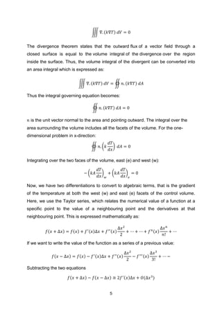
The East boundary node is:
Figure 5: volume at the east boundary
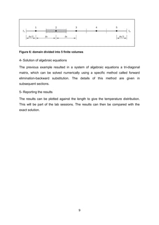
If we use a 5 finite volumes as shown in Figure 6; points from 2 to 4 are node points,
point 1 is the west point, and point 5 is the east point. This will result in 5 linear
algebraic equations in 5 unknowns. This system of algebraic equations can be
written in matrix form as:
[ ] [ ] [ ]
Note that all the equations were multiplied by -1 to get the above matrix.
W
𝑇𝐵
w P e
Δ𝑥⁄
Δ𝑥

9. 9
Figure 6: domain divided into 5 finite volumes
4- Solution of algebraic equations
The previous example resulted in a system of algebraic equations a tri-diagonal
matrix, which can be solved numerically using a specific method called forward
elimination-backward substitution. The details of this method are given in
subsequent sections.
5- Reporting the results
The results can be plotted against the length to give the temperature distribution.
This will be part of the lab sessions. The results can then be compared with the
exact solution.