Download free for 30 days
Sign in
Upload
Language (EN)
Support
Business
Mobile
Social Media
Marketing
Technology
Art & Photos
Career
Design
Education
Presentations & Public Speaking
Government & Nonprofit
Healthcare
Internet
Law
Leadership & Management
Automotive
Engineering
Software
Recruiting & HR
Retail
Sales
Services
Science
Small Business & Entrepreneurship
Food
Environment
Economy & Finance
Data & Analytics
Investor Relations
Sports
Spiritual
News & Politics
Travel
Self Improvement
Real Estate
Entertainment & Humor
Health & Medicine
Devices & Hardware
Lifestyle
Change Language
Language
English
Español
Português
Français
Deutsche
Cancel
Save
EN
Uploaded by
ssuser86189f
PPT, PDF
3 views
Introygffhhffduction_to_Aerodynamics1.pptx
Introduction_to_Aerodynamics1.pptx
Engineering
◦
Read more
0
Save
Share
Embed
Embed presentation
Download
Download to read offline
1
/ 61
2
/ 61
3
/ 61
4
/ 61
5
/ 61
6
/ 61
7
/ 61
8
/ 61
9
/ 61
10
/ 61
11
/ 61
12
/ 61
13
/ 61
14
/ 61
15
/ 61
16
/ 61
17
/ 61
18
/ 61
19
/ 61
20
/ 61
21
/ 61
22
/ 61
23
/ 61
24
/ 61
25
/ 61
26
/ 61
27
/ 61
28
/ 61
29
/ 61
30
/ 61
31
/ 61
32
/ 61
33
/ 61
34
/ 61
35
/ 61
36
/ 61
37
/ 61
38
/ 61
39
/ 61
40
/ 61
41
/ 61
42
/ 61
43
/ 61
44
/ 61
45
/ 61
46
/ 61
47
/ 61
48
/ 61
49
/ 61
50
/ 61
51
/ 61
52
/ 61
53
/ 61
54
/ 61
55
/ 61
56
/ 61
57
/ 61
58
/ 61
59
/ 61
60
/ 61
61
/ 61
More Related Content
PPSX
multiphase flow modeling and simulation ,Pouriya Niknam , UNIFI
by
Pouriya Niknam
PDF
multiphase flow, applied computational fluid dynamics
by
gerardopalmaalvarez1
PDF
Chp18
by
Chethan Reddy
PDF
Fluent 13.0 lecture09-physics
by
Rashed Kaiser
PPTX
01 multiphaseflows-fundamental definitions.pptx
by
AjeetPattnaik1
PPTX
Multiphase model
by
Nasser Touliemat
PDF
01 multiphase flows- fundamental definitions
by
Mohammad Jadidi
PPTX
CFD Modeling of Multiphase Flow. Focus on Liquid-Solid Flow
by
Luis Ram Rojas-Sol
multiphase flow modeling and simulation ,Pouriya Niknam , UNIFI
by
Pouriya Niknam
multiphase flow, applied computational fluid dynamics
by
gerardopalmaalvarez1
Chp18
by
Chethan Reddy
Fluent 13.0 lecture09-physics
by
Rashed Kaiser
01 multiphaseflows-fundamental definitions.pptx
by
AjeetPattnaik1
Multiphase model
by
Nasser Touliemat
01 multiphase flows- fundamental definitions
by
Mohammad Jadidi
CFD Modeling of Multiphase Flow. Focus on Liquid-Solid Flow
by
Luis Ram Rojas-Sol
Similar to Introygffhhffduction_to_Aerodynamics1.pptx
PDF
Fluent-v6.2.01 - Software CFD.pdf
by
ibskonversienergi
PPTX
phenomena of multiphase reactor performance
by
prmsgr0
PPTX
Multiphase models
by
Hamed Hoorijani
PPTX
CFD Lecture (8/8): CFD in Chemical Systems
by
Abhishek Jain
PPTX
A Comprehensive Study of Multiphase Flow through Annular Pipe using CFD Approach
by
Raian Nur Islam
PDF
Multiphase Flow Modeling
by
iMentor Education
PDF
Tank
by
Kota Sridhar
PPT
Fluent.05.turbulencef77g7g7g7gg7g7g7g7g7g7g
by
224me8002
PDF
Case studing
by
Mohsen Salehi
PDF
00 multiphase flows - intorduction
by
Mohammad Jadidi
PDF
The VOF model in FLUENT adv-multiphase-4-vof.pdf
by
ShyamalBhunia2
PDF
Computational Models For Polydisperse Particulate And Multiphase Systems Dani...
by
droniapoux
PDF
Multiphase Flow Handbook 1st Edition Clayton T. Crowe (Editor)
by
dhonzrouvas
PPT
Simulation of Steam Coal Gasifier
by
egepaul
PDF
Introduction to Multiphase Flow Modeling
by
iMentor Education
PDF
Chapter 10. VOF Free Surface Model
by
Ray Young
PPTX
Chapter 4 Flowing Fluids Pressure Variations (1).pptx
by
DavidAji1
PDF
Manuscript
by
Ming Ma
PDF
pof
by
Ming Ma
PDF
Introduction to Coupled CFD-DEM Modeling
by
Khusro Kamaluddin
Fluent-v6.2.01 - Software CFD.pdf
by
ibskonversienergi
phenomena of multiphase reactor performance
by
prmsgr0
Multiphase models
by
Hamed Hoorijani
CFD Lecture (8/8): CFD in Chemical Systems
by
Abhishek Jain
A Comprehensive Study of Multiphase Flow through Annular Pipe using CFD Approach
by
Raian Nur Islam
Multiphase Flow Modeling
by
iMentor Education
Tank
by
Kota Sridhar
Fluent.05.turbulencef77g7g7g7gg7g7g7g7g7g7g
by
224me8002
Case studing
by
Mohsen Salehi
00 multiphase flows - intorduction
by
Mohammad Jadidi
The VOF model in FLUENT adv-multiphase-4-vof.pdf
by
ShyamalBhunia2
Computational Models For Polydisperse Particulate And Multiphase Systems Dani...
by
droniapoux
Multiphase Flow Handbook 1st Edition Clayton T. Crowe (Editor)
by
dhonzrouvas
Simulation of Steam Coal Gasifier
by
egepaul
Introduction to Multiphase Flow Modeling
by
iMentor Education
Chapter 10. VOF Free Surface Model
by
Ray Young
Chapter 4 Flowing Fluids Pressure Variations (1).pptx
by
DavidAji1
Manuscript
by
Ming Ma
pof
by
Ming Ma
Introduction to Coupled CFD-DEM Modeling
by
Khusro Kamaluddin
Recently uploaded
PDF
Plasticity and Structure of Soil/Atterberg Limits.pdf
by
MahmoodKhalid11
PDF
Computer Graphics Fundamentals (v0p1) - DannyJiang
by
Danny Jiang
PPTX
Batch-1(End Semester) Student Of Shree Durga Tech. PPT.pptx
by
rashesw1122s
PDF
Shear Strength of Soil (Direct shear test).pdf
by
MahmoodKhalid11
PDF
Infinite Sequence and Series: It Includes basic Sequence and Series
by
DynamicDomain1
PPTX
Value engineering and cost analysis with case study
by
hp9879098082
PPTX
What Green Hydrogen Is Definition: Hydrogen produced via electrolysis of wate...
by
Thit57
PDF
engineering management chapter 5 ppt presentation
by
ericaangelatoledo06
PPT
Momentum and collisions in physics or engineering
by
azizrahmanhakimi
PPTX
Why TPM Succeeds in Some Plants and Struggles in Others | MaintWiz
by
MaintWiz Technologies Private Limited
PPTX
uADPF Topology_SFP requirements_locked slides.pptx
by
Md Bellal Hossain
PDF
CME397 SURFACE ENGINEERING UNIT 2 FULL NOTES
by
karthi keyan
PDF
PROBLEM SLOVING AND PYTHON PROGRAMMING UNIT 3.pdf
by
A R SIVANESH M.E., QIP-PG (Cyber Security)., (Ph.D)
PPTX
traffic safety section seven (Traffic Control and Management) of Act
by
azeRakeshSunariMagar
PPTX
Day 3 Module 5_Optical fiber Network (operation and management).pptx
by
SachayaG
PDF
Rajesh Prasad- Brief Profile with educational, professional highlights
by
Rajesh Prasad
PDF
Soil Compressibility (Elastic Settlement).pdf
by
MahmoodKhalid11
PDF
Industrial Tools Manufacturers In India : Torso Tools
by
torsotools8
PPTX
How Does LNG Regasification Work | INOXCVA
by
INOXCVA
PDF
Decision-Support-Systems-and-Decision-Making-Processes.pdf
by
PatankarNikhil
Plasticity and Structure of Soil/Atterberg Limits.pdf
by
MahmoodKhalid11
Computer Graphics Fundamentals (v0p1) - DannyJiang
by
Danny Jiang
Batch-1(End Semester) Student Of Shree Durga Tech. PPT.pptx
by
rashesw1122s
Shear Strength of Soil (Direct shear test).pdf
by
MahmoodKhalid11
Infinite Sequence and Series: It Includes basic Sequence and Series
by
DynamicDomain1
Value engineering and cost analysis with case study
by
hp9879098082
What Green Hydrogen Is Definition: Hydrogen produced via electrolysis of wate...
by
Thit57
engineering management chapter 5 ppt presentation
by
ericaangelatoledo06
Momentum and collisions in physics or engineering
by
azizrahmanhakimi
Why TPM Succeeds in Some Plants and Struggles in Others | MaintWiz
by
MaintWiz Technologies Private Limited
uADPF Topology_SFP requirements_locked slides.pptx
by
Md Bellal Hossain
CME397 SURFACE ENGINEERING UNIT 2 FULL NOTES
by
karthi keyan
PROBLEM SLOVING AND PYTHON PROGRAMMING UNIT 3.pdf
by
A R SIVANESH M.E., QIP-PG (Cyber Security)., (Ph.D)
traffic safety section seven (Traffic Control and Management) of Act
by
azeRakeshSunariMagar
Day 3 Module 5_Optical fiber Network (operation and management).pptx
by
SachayaG
Rajesh Prasad- Brief Profile with educational, professional highlights
by
Rajesh Prasad
Soil Compressibility (Elastic Settlement).pdf
by
MahmoodKhalid11
Industrial Tools Manufacturers In India : Torso Tools
by
torsotools8
How Does LNG Regasification Work | INOXCVA
by
INOXCVA
Decision-Support-Systems-and-Decision-Making-Processes.pdf
by
PatankarNikhil
Introygffhhffduction_to_Aerodynamics1.pptx
1.
© Fluent Inc.
12/26/25 1 Fluent Software Training TRN-99-003 Modeling Multiphase Flows
2.
© Fluent Inc.
12/26/25 2 Fluent Software Training TRN-99-003 Outline Definitions; Examples of flow regimes Description of multiphase models in FLUENT 5 and FLUENT 4.5 How to choose the correct model for your application Summary and guidelines
3.
© Fluent Inc.
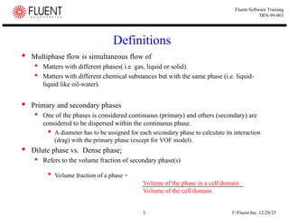
12/26/25 3 Fluent Software Training TRN-99-003 Definitions Multiphase flow is simultaneous flow of Matters with different phases( i.e. gas, liquid or solid). Matters with different chemical substances but with the same phase (i.e. liquid- liquid like oil-water). Primary and secondary phases One of the phases is considered continuous (primary) and others (secondary) are considered to be dispersed within the continuous phase. A diameter has to be assigned for each secondary phase to calculate its interaction (drag) with the primary phase (except for VOF model). Dilute phase vs. Dense phase; Refers to the volume fraction of secondary phase(s) Volume fraction of a phase = Volume of the phase in a cell/domain Volume of the cell/domain
4.
© Fluent Inc.
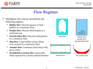
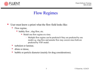
12/26/25 4 Fluent Software Training TRN-99-003 Flow Regimes Multiphase flow can be classified by the following regimes: Bubbly flow: Discrete gaseous or fluid bubbles in a continuous fluid Droplet flow: Discrete fluid droplets in a continuous gas Particle-laden flow: Discrete solid particles in a continuous fluid Slug flow: Large bubbles (nearly filling cross-section) in a continuous fluid Annular flow: Continuous fluid along walls, gas in center Stratified/free-surface flow: Immiscible fluids separated by a clearly-defined interface bubbly flow droplet flow particle-laden flow slug flow annular flow free-surface flow
5.
© Fluent Inc.
12/26/25 5 Fluent Software Training TRN-99-003 Flow Regimes User must know a priori what the flow field looks like: Flow regime, bubbly flow , slug flow, etc. Model one flow regime at a time. – Multiple flow regime can be predicted if they are predicted by one model e.g. slug flow and annular flow may coexist since both are predicted by VOF model. turbulent or laminar, dilute or dense, bubble or particle diameter (mainly for drag considerations).
6.
© Fluent Inc.
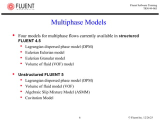
12/26/25 6 Fluent Software Training TRN-99-003 Multiphase Models Four models for multiphase flows currently available in structured FLUENT 4.5 Lagrangian dispersed phase model (DPM) Eulerian Eulerian model Eulerian Granular model Volume of fluid (VOF) model Unstructured FLUENT 5 Lagrangian dispersed phase model (DPM) Volume of fluid model (VOF) Algebraic Slip Mixture Model (ASMM) Cavitation Model
7.
© Fluent Inc.
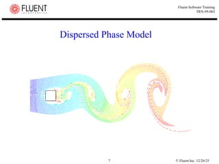
12/26/25 7 Fluent Software Training TRN-99-003 Dispersed Phase Model
8.
© Fluent Inc.
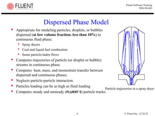
12/26/25 8 Fluent Software Training TRN-99-003 Dispersed Phase Model Appropriate for modeling particles, droplets, or bubbles dispersed (at low volume fraction; less than 10%) in continuous fluid phase: Spray dryers Coal and liquid fuel combustion Some particle-laden flows Computes trajectories of particle (or droplet or bubble) streams in continuous phase. Computes heat, mass, and momentum transfer between dispersed and continuous phases. Neglects particle-particle interaction. Particles loading can be as high as fluid loading Computes steady and unsteady (FLUENT 5) particle tracks. Particle trajectories in a spray dryer
9.
© Fluent Inc.
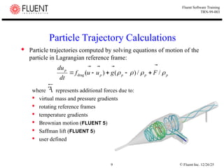
12/26/25 9 Fluent Software Training TRN-99-003 Particle trajectories computed by solving equations of motion of the particle in Lagrangian reference frame: where represents additional forces due to: virtual mass and pressure gradients rotating reference frames temperature gradients Brownian motion (FLUENT 5) Saffman lift (FLUENT 5) user defined Particle Trajectory Calculations p p p p p F g u u f dt u d / / ) ( ) ( drag
10.
© Fluent Inc.
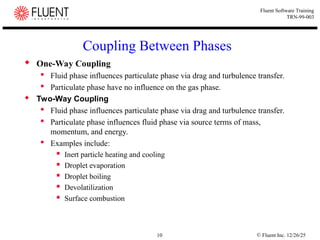
12/26/25 10 Fluent Software Training TRN-99-003 Coupling Between Phases One-Way Coupling Fluid phase influences particulate phase via drag and turbulence transfer. Particulate phase have no influence on the gas phase. Two-Way Coupling Fluid phase influences particulate phase via drag and turbulence transfer. Particulate phase influences fluid phase via source terms of mass, momentum, and energy. Examples include: Inert particle heating and cooling Droplet evaporation Droplet boiling Devolatilization Surface combustion
11.
© Fluent Inc.
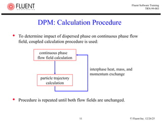
12/26/25 11 Fluent Software Training TRN-99-003 To determine impact of dispersed phase on continuous phase flow field, coupled calculation procedure is used: Procedure is repeated until both flow fields are unchanged. DPM: Calculation Procedure continuous phase flow field calculation particle trajectory calculation interphase heat, mass, and momentum exchange
12.
© Fluent Inc.
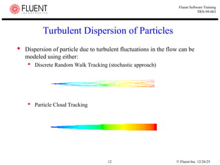
12/26/25 12 Fluent Software Training TRN-99-003 Turbulent Dispersion of Particles Dispersion of particle due to turbulent fluctuations in the flow can be modeled using either: Discrete Random Walk Tracking (stochastic approach) Particle Cloud Tracking
13.
© Fluent Inc.
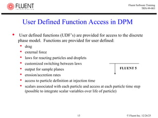
12/26/25 13 Fluent Software Training TRN-99-003 User Defined Function Access in DPM User defined functions (UDF’s) are provided for access to the discrete phase model. Functions are provided for user defined: drag external force laws for reacting particles and droplets customized switching between laws output for sample planes erosion/accretion rates access to particle definition at injection time scalars associated with each particle and access at each particle time step (possible to integrate scalar variables over life of particle) FLUENT 5
14.
© Fluent Inc.
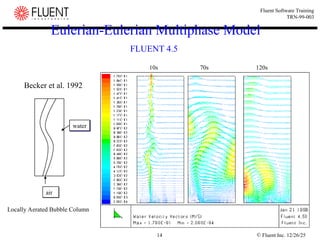
12/26/25 14 Fluent Software Training TRN-99-003 Eulerian-Eulerian Multiphase Model FLUENT 4.5 10s 70s 120s water air Becker et al. 1992 Locally Aerated Bubble Column
15.
© Fluent Inc.
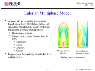
12/26/25 15 Fluent Software Training TRN-99-003 Eulerian Multiphase Model Appropriate for modeling gas-liquid or liquid-liquid flows (droplets or bubbles of secondary phase(s) dispersed in continuous fluid phase (primary phase)) where: Phases mix or separate Bubble/droplet volume fractions from 0 to 100% Evaporation Boiling Separators Aeration Inappropriate for modeling stratified or free- surface flows. Volume fraction of water Stream function contours for water Boiling water in a container
16.
© Fluent Inc.
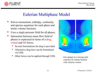
12/26/25 16 Fluent Software Training TRN-99-003 Eulerian Multiphase Model Solves momentum, enthalpy, continuity, and species equations for each phase and tracks volume fractions. Uses a single pressure field for all phases. Interaction between mean flow field of phases is expressed in terms of a drag, virtual and lift forces. Several formulations for drag is provided. Alternative drag laws can be formulated via UDS. Other forces can be applied through UDS. Gas sparger in a mixing tank: contours of volume fraction with velocity vectors
17.
© Fluent Inc.
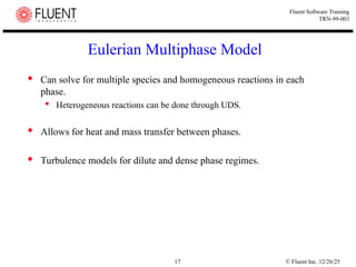
12/26/25 17 Fluent Software Training TRN-99-003 Eulerian Multiphase Model Can solve for multiple species and homogeneous reactions in each phase. Heterogeneous reactions can be done through UDS. Allows for heat and mass transfer between phases. Turbulence models for dilute and dense phase regimes.
18.
© Fluent Inc.
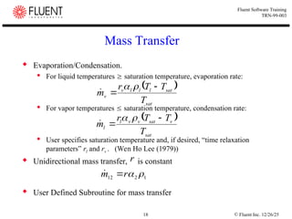
12/26/25 18 Fluent Software Training TRN-99-003 Mass Transfer Evaporation/Condensation. For liquid temperatures saturation temperature, evaporation rate: For vapor temperatures saturation temperature, condensation rate: User specifies saturation temperature and, if desired, “time relaxation parameters” rl and rv . (Wen Ho Lee (1979)) Unidirectional mass transfer, is constant User Defined Subroutine for mass transfer sat sat l l l v v T T T r m sat v sat v v l l T T T r m 1 2 12 r m r
19.
© Fluent Inc.
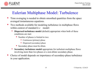
12/26/25 19 Fluent Software Training TRN-99-003 Eulerian Multiphase Model: Turbulence Time averaging is needed to obtain smoothed quantities from the space averaged instantaneous equations. Two methods available for modeling turbulence in multiphase flows within context of standard k-model: Dispersed turbulence model (default) appropriate when both of these conditions are met: Number of phases is limited to two: Continuous (primary) phase Dispersed (secondary) phase Secondary phase must be dilute. Secondary turbulence model appropriate for turbulent multiphase flows involving more than two phases or a non-dilute secondary phase. Choice of model depends on importance of secondary-phase turbulence in your application.
20.
© Fluent Inc.
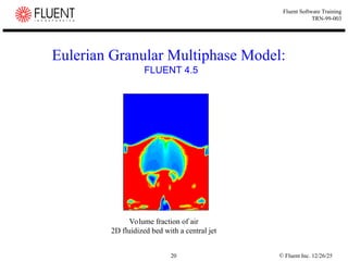
12/26/25 20 Fluent Software Training TRN-99-003 Eulerian Granular Multiphase Model: FLUENT 4.5 Volume fraction of air 2D fluidized bed with a central jet
21.
© Fluent Inc.
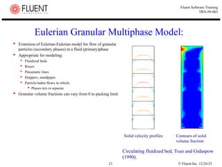
12/26/25 21 Fluent Software Training TRN-99-003 Eulerian Granular Multiphase Model: Extension of Eulerian-Eulerian model for flow of granular particles (secondary phases) in a fluid (primary)phase Appropriate for modeling: Fluidized beds Risers Pneumatic lines Hoppers, standpipes Particle-laden flows in which: Phases mix or separate Granular volume fractions can vary from 0 to packing limit Circulating fluidized bed, Tsuo and Gidaspow (1990). Solid velocity profiles Contours of solid volume fraction
22.
© Fluent Inc.
12/26/25 22 Fluent Software Training TRN-99-003 Eulerian Granular Multiphase Model: Overview The fluid phase must be assigned as the primary phase. Multiple solid phase can be used to represent size distribution. Can calculate granular temperature (solids fluctuating energy) for each solid phase. Calculates a solids pressure field for each solid phase. All phases share fluid pressure field. Solids pressure controls the solids packing limit Solids pressure, granular temperature conductivity, shear and bulk viscosity can be derived based on several kinetic theory formulations. Gidaspow -good for dense fluidized bed applications Syamlal -good for a wide range of applications Sinclair -good for dilute and dense pneumatic transport lines and risers
23.
© Fluent Inc.
12/26/25 23 Fluent Software Training TRN-99-003 Eulerian Granular Multiphase Model Frictional viscosity pushes the limit into the plastic regime. Hoppers, standpipes Several choice of drag laws: Drag laws can be modified using UDS. Heat transfer between phases is the same as in Eulerian/Eulerian multiphase model. Only unidirectional mass transfer model is available. Rate of mass transfer can be modified using UDS. Homogeneous reaction can be modeled. Heterogeneous reaction can be modeled using UDS. Can solve for enthalpy and multiple species for each phase. Physically based models for solid momentum and granular temperature boundary conditions at the wall. Turbulence treatment is the same as in Eulerian-Eulerian model Sinclair model provides additional turbulence model for solid phase
24.
© Fluent Inc.
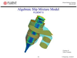
12/26/25 24 Fluent Software Training TRN-99-003 Algebraic Slip Mixture Model FLUENT 5 Courtesy of Fuller Company
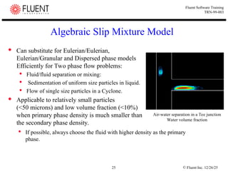
25.
© Fluent Inc.
12/26/25 25 Fluent Software Training TRN-99-003 Algebraic Slip Mixture Model Can substitute for Eulerian/Eulerian, Eulerian/Granular and Dispersed phase models Efficiently for Two phase flow problems: Fluid/fluid separation or mixing: Sedimentation of uniform size particles in liquid. Flow of single size particles in a Cyclone. Applicable to relatively small particles (<50 microns) and low volume fraction (<10%) when primary phase density is much smaller than the secondary phase density. Air-water separation in a Tee junction Water volume fraction If possible, always choose the fluid with higher density as the primary phase.
26.
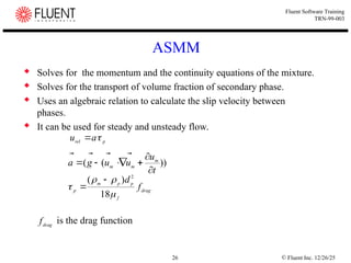
© Fluent Inc.
12/26/25 26 Fluent Software Training TRN-99-003 Solves for the momentum and the continuity equations of the mixture. Solves for the transport of volume fraction of secondary phase. Uses an algebraic relation to calculate the slip velocity between phases. It can be used for steady and unsteady flow. is the drag function ASMM p rel a u )) ( ( t u u u g a m m m drag f p p m p f d 18 ) ( 2 drag f
27.
© Fluent Inc.
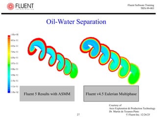
12/26/25 27 Fluent Software Training TRN-99-003 Oil-Water Separation Fluent 5 Results with ASMM Fluent v4.5 Eulerian Multiphase Courtesy of Arco Exploration & Production Technology Dr. Martin de Tezanos Pinto
28.
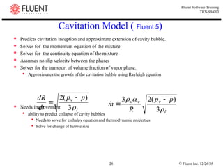
© Fluent Inc.
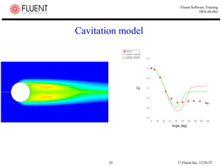
12/26/25 28 Fluent Software Training TRN-99-003 Cavitation Model ( Fluent 5) Predicts cavitation inception and approximate extension of cavity bubble. Solves for the momentum equation of the mixture Solves for the continuity equation of the mixture Assumes no slip velocity between the phases Solves for the transport of volume fraction of vapor phase. Approximates the growth of the cavitation bubble using Rayleigh equation Needs improvement: ability to predict collapse of cavity bubbles Needs to solve for enthalpy equation and thermodynamic properties Solve for change of bubble size l v p p dt dR 3 ) ( 2 l v v v p p R m 3 ) ( 2 3
29.
© Fluent Inc.
12/26/25 29 Fluent Software Training TRN-99-003 Cavitation model
30.
© Fluent Inc.
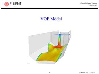
12/26/25 30 Fluent Software Training TRN-99-003 VOF Model
31.
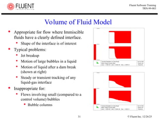
© Fluent Inc.
12/26/25 31 Fluent Software Training TRN-99-003 Volume of Fluid Model Appropriate for flow where Immiscible fluids have a clearly defined interface. Shape of the interface is of interest Typical problems: Jet breakup Motion of large bubbles in a liquid Motion of liquid after a dam break (shown at right) Steady or transient tracking of any liquid-gas interface Inappropriate for: Flows involving small (compared to a control volume) bubbles Bubble columns
32.
© Fluent Inc.
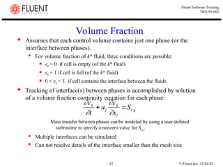
12/26/25 32 Fluent Software Training TRN-99-003 Volume Fraction Assumes that each control volume contains just one phase (or the interface between phases). For volume fraction of kth fluid, three conditions are possible: k = 0 if cell is empty (of the kth fluid) k = 1 if cell is full (of the kth fluid) 0 < k < 1 if cell contains the interface between the fluids Tracking of interface(s) between phases is accomplished by solution of a volume fraction continuity equation for each phase: Mass transfer between phases can be modeled by using a user-defined subroutine to specify a nonzero value for Sk . Multiple interfaces can be simulated Can not resolve details of the interface smaller than the mesh size k j k i k t u x S
33.
© Fluent Inc.
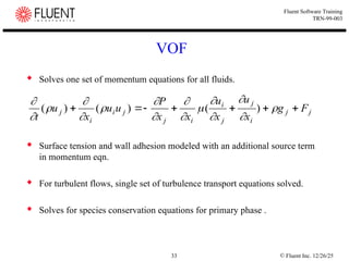
12/26/25 33 Fluent Software Training TRN-99-003 VOF Solves one set of momentum equations for all fluids. Surface tension and wall adhesion modeled with an additional source term in momentum eqn. For turbulent flows, single set of turbulence transport equations solved. Solves for species conservation equations for primary phase . j j i j j i i j j i i j F g x u x u x x P u u x u t ) ( ) ( ) (
34.
© Fluent Inc.
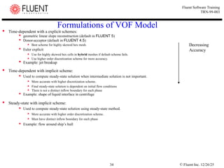
12/26/25 34 Fluent Software Training TRN-99-003 Formulations of VOF Model Time-dependent with a explicit schemes: geometric linear slope reconstruction (default in FLUENT 5) Donor-acceptor (default in FLUENT 4.5) Best scheme for highly skewed hex mesh. Euler explicit Use for highly skewed hex cells in hybrid meshes if default scheme fails. Use higher order discretization scheme for more accuracy. Example: jet breakup Time-dependent with implicit scheme: Used to compute steady-state solution when intermediate solution is not important. More accurate with higher discretization scheme. Final steady-state solution is dependent on initial flow conditions There is not a distinct inflow boundary for each phase Example: shape of liquid interface in centrifuge Steady-state with implicit scheme: Used to compute steady-state solution using steady-state method. More accurate with higher order discretization scheme. Must have distinct inflow boundary for each phase Example: flow around ship’s hull Decreasing Accuracy
35.
© Fluent Inc.
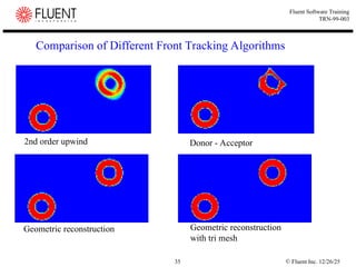
12/26/25 35 Fluent Software Training TRN-99-003 Comparison of Different Front Tracking Algorithms 2nd order upwind Donor - Acceptor Geometric reconstruction Geometric reconstruction with tri mesh
36.
© Fluent Inc.
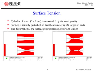
12/26/25 36 Fluent Software Training TRN-99-003 Surface Tension Cylinder of water (5 x 1 cm) is surrounded by air in no gravity Surface is initially perturbed so that the diameter is 5% larger on ends The disturbance at the surface grows because of surface tension
37.
© Fluent Inc.
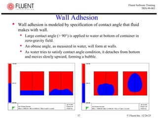
12/26/25 37 Fluent Software Training TRN-99-003 Wall Adhesion Wall adhesion is modeled by specification of contact angle that fluid makes with wall. Large contact angle (> 90°) is applied to water at bottom of container in zero-gravity field. An obtuse angle, as measured in water, will form at walls. As water tries to satisfy contact angle condition, it detaches from bottom and moves slowly upward, forming a bubble.
38.
© Fluent Inc.
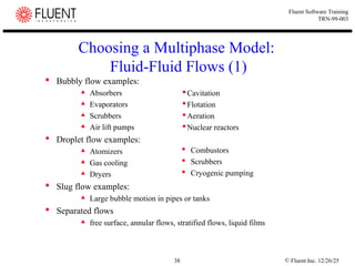
12/26/25 38 Fluent Software Training TRN-99-003 Choosing a Multiphase Model: Fluid-Fluid Flows (1) Bubbly flow examples: Absorbers Evaporators Scrubbers Air lift pumps Droplet flow examples: Atomizers Gas cooling Dryers Slug flow examples: Large bubble motion in pipes or tanks Separated flows free surface, annular flows, stratified flows, liquid films Cavitation Flotation Aeration Nuclear reactors Combustors Scrubbers Cryogenic pumping
39.
© Fluent Inc.
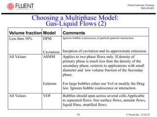
12/26/25 39 Fluent Software Training TRN-99-003 Choosing a Multiphase Model: Gas-Liquid Flows (2) Volume fraction Model Comments Less than 10% DPM Cavitation Ignores bubble coalescence or particle-particle interaction. Inception of cavitation and its approximate extension. All Values ASMM Eulerian Applies to two phase flows only. If density of primary phase is much less than the density of the secondary phase, restricts to applications with small diameter and low volume fraction of the Seconday phase. For large bubbles either use Vof or modify the Drag law. Ignores bubble coalescence or interaction. All Values VOF Bubbles should span across several cells.Applicable to separated flows: free surface flows, annular flows, liquid films, stratified flows.
40.
© Fluent Inc.
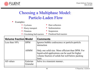
12/26/25 40 Fluent Software Training TRN-99-003 Choosing a Multiphase Model: Particle-Laden Flow Examples: Cyclones Slurry transport Flotation Circulating bed reactors Dust collectors Sedimentation Suspension Fluidized bed reactors Volume fraction Model Comments Less than 10% DPM ASMM Ignores bubble coalescence or particle-particle interaction Only one solid size. More efficient than DPM. For liquid-solid applications can be used for higher volume fraction of solids but well below packing limit. All values Eulerian Granular Solve in a transient manner..
41.
© Fluent Inc.
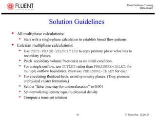
12/26/25 41 Fluent Software Training TRN-99-003 Solution Guidelines All multiphase calculations: Start with a single-phase calculation to establish broad flow patterns. Eulerian multiphase calculations: Use COPY-PHASE-VELOCITIES to copy primary phase velocities to secondary phases. Patch secondary volume fraction(s) as an initial condition. For a single outflow, use OUTLET rather than PRESSURE-INLET; for multiple outflow boundaries, must use PRESSURE-INLET for each. For circulating fluidized beds, avoid symmetry planes. (They promote unphysical cluster formation.) Set the “false time step for underrelaxation” to 0.001 Set normalizing density equal to physical density Compute a transient solution
42.
© Fluent Inc.
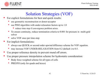
12/26/25 42 Fluent Software Training TRN-99-003 Solution Strategies (VOF) For explicit formulations for best and quick results: use geometric reconstruction or donor-acceptor use PISO algorithm with under-relaxation factors up to 1.0 reduce time step if convergence problem arises. To ensure continuity, reduce termination criteria to 0.001 for pressure in multi-grid solver solve VOF once per time-step For implicit formulations: always use QUICK or second order upwind difference scheme for VOF equation. may increase VOF UNDER-RELAXATION from 0.2 (default ) to 0.5. Use proper reference density to prevent round off errors. Use proper pressure interpolation scheme for hydrostatic consideration: Body force weighted scheme for all types of cells PRESTO (only for quads and hexes)
43.
© Fluent Inc.
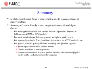
12/26/25 43 Fluent Software Training TRN-99-003 Summary Modeling multiphase flows is very complex, due to interdependence of many variables. Accuracy of results directly related to appropriateness of model you choose: For most applications with low volume fraction of particles, droplets, or bubbles, use ASMM or DPM model . For particle-laden flows, Eulerian granular multiphase model is best. For separated gas-liquid flows (stratified, free-surface, etc.) VOF model is best. For general, complex gas-liquid flows involving multiple flow regimes: Select aspect of flow that is of most interest. Choose model that is most appropriate. Accuracy of results will not be as good as for others, since selected physical model will be valid only for some flow regimes.
44.
© Fluent Inc.
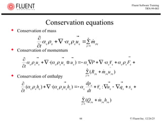
12/26/25 44 Fluent Software Training TRN-99-003 Conservation equations Conservation of mass Conservation of momentum Conservation of enthalpy q q q q q q q q q q q q q F P u u u t ) ( n p pq q q q q q m u t 1 ) ( 1 pq pq n p pq u m R q q q k q q q q q q q q q s q u dt dp h u h t . : ) ( ) ( ) ( 1 pq pq n p pq h m Q
45.
© Fluent Inc.
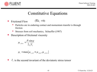
12/26/25 45 Fluent Software Training TRN-99-003 Constitutive Equations Frictional Flow Particles are in enduring contact and momentum transfer is through friction Stresses from soil mechanics, Schaeffer (1987) Description of frictional viscosity is the second invariant of the deviatoric stress tensor frict s kin s coll s s , , , , max ) 0 ( s u 2 , 2 sin I Ps frict s 2 I
46.
© Fluent Inc.
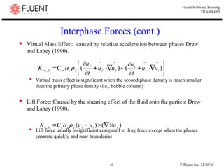
12/26/25 46 Fluent Software Training TRN-99-003 Interphase Forces (cont.) Virtual Mass Effect: caused by relative acceleration between phases Drew and Lahey (1990). Virtual mass effect is significant when the second phase density is much smaller than the primary phase density (i.e., bubble column) Lift Force: Caused by the shearing effect of the fluid onto the particle Drew and Lahey (1990). Lift force usually insignificant compared to drag force except when the phases separate quickly and near boundaries ) ( ) ( , s s s f f f f s vm fs vm u u t u u u t u C K ) ( ) ( , f s f f s L fs k u u u C K
47.
© Fluent Inc.
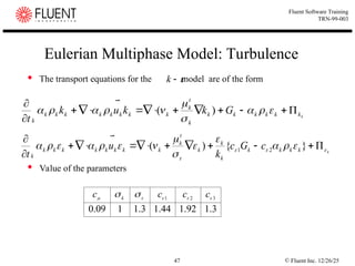
12/26/25 47 Fluent Software Training TRN-99-003 Eulerian Multiphase Model: Turbulence The transport equations for the model are of the form Value of the parameters k k k k k k k k k t k k k k k k k k k k G k k u k t ) ( k k k k k k k k t k k k k k k k k k k c G c k u t } { ) ( 2 1 3 . 1 92 . 1 44 . 1 3 . 1 1 09 . 0 3 2 1 c c c c k
48.
© Fluent Inc.
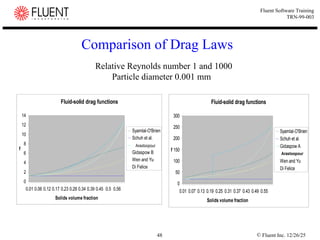
12/26/25 48 Fluent Software Training TRN-99-003 Comparison of Drag Laws Fluid-solid drag functions 0 2 4 6 8 10 12 14 0.01 0.06 0.12 0.17 0.23 0.28 0.34 0.39 0.45 0.5 0.56 Solids volume fraction f Syamlal-O'Brien Schuh et al. Gidaspow A Gidaspow B Wen and Yu Di Felice Fluid-solid drag functions 0 50 100 150 200 250 300 0.01 0.07 0.13 0.19 0.25 0.31 0.37 0.43 0.49 0.55 Solids volume fraction f Syamlal-O'Brien Schuh et al. Gidaspow A Gidaspow B Wen and Yu Di Felice Relative Reynolds number 1 and 1000 Particle diameter 0.001 mm Arastoopour Arastoopour
49.
© Fluent Inc.
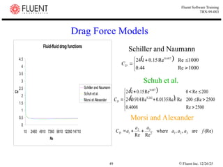
12/26/25 49 Fluent Software Training TRN-99-003 Drag Force Models Fluid-fluid drag functions 0 0.5 1 1.5 2 2.5 3 3.5 4 4.5 10 2460 4910 7360 9810 12260 14710 Re Cd Schiller and Naumann Schuh et al. Morsi et Alexander 1000 Re 44 . 0 1000 Re Re 15 . 0 1 24 687 . 0 D C 2500 Re 4008 . 0 2500 Re 200 Re / Re 0135 . 0 Re 914 . 0 24 200 Re 0 Re 15 . 0 1 24 282 . 0 687 . 0 D C (Re) are , , where Re Re 3 2 1 2 3 2 1 f a a a a a a CD Schiller and Naumann Schuh et al. Morsi and Alexander
50.
© Fluent Inc.
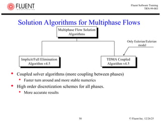
12/26/25 50 Fluent Software Training TRN-99-003 Solution Algorithms for Multiphase Flows Coupled solver algorithms (more coupling between phases) Faster turn around and more stable numerics High order discretization schemes for all phases. More accurate results Implicit/Full Elimination Algorithm v4.5 Implicit/Full Elimination Algorithm v4.5 TDMA Coupled Algorithm v4.5 TDMA Coupled Algorithm v4.5 Multiphase Flow Solution Algorithms Multiphase Flow Solution Algorithms Only Eulerian/Eulerian model
51.
© Fluent Inc.
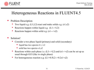
12/26/25 51 Fluent Software Training TRN-99-003 Heterogeneous Reactions in FLUENT4.5 Problem Description Two liquid e.g. (L1,L2) react and make solids e.g. (s1,s2) Reactions happen within liquid e.g. (L1-->L2) Reactions happen within solid e.g. (s1--->s2) Solution! Consider a two phase liquid (primary) and solid (secondary) liquid has two species L1, L2 solid has two species s1,s2 Reactions within each phase i.e. (L1-->L2) and (s1-->s2) can be set up as usual through GUI (like in single phase) For heterogeneous reaction e.g. (L1+0.5L2-->0.2s1+s2)
52.
© Fluent Inc.
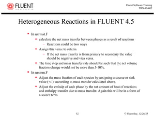
12/26/25 52 Fluent Software Training TRN-99-003 Heterogeneous Reactions in FLUENT 4.5 In usrmst.F calculate the net mass transfer between phases as a result of reactions – Reactions could be two ways Assign this value to suterm – If the net mass transfer is from primary to secondary the value should be negative and vica versa. The time step and mass transfer rate should be such that the net volume fraction change would not be more than 5-10%. In urstrm.F Adjust the mass fraction of each species by assigning a source or sink value (+/-) according to mass transfer calculated above. Adjust the enthalp of each phase by the net amount of heat of reactions and enthalpy transfer due to mass transfer. Again this will be in a form of a source term.
53.
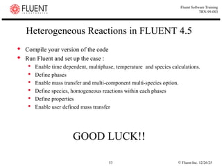
© Fluent Inc.
12/26/25 53 Fluent Software Training TRN-99-003 Heterogeneous Reactions in FLUENT 4.5 Compile your version of the code Run Fluent and set up the case : Enable time dependent, multiphase, temperature and species calculations. Define phases Enable mass transfer and multi-component multi-species option. Define species, homogeneous reactions within each phases Define properties Enable user defined mass transfer GOOD LUCK!!
54.
© Fluent Inc.
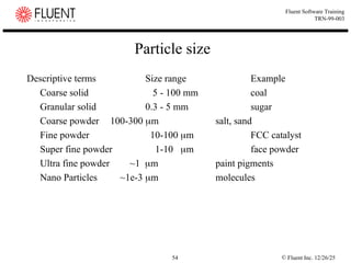
12/26/25 54 Fluent Software Training TRN-99-003 Particle size Descriptive terms Size range Example Coarse solid 5 - 100 mm coal Granular solid 0.3 - 5 mm sugar Coarse powder 100-300 m salt, sand Fine powder 10-100 m FCC catalyst Super fine powder 1-10 m face powder Ultra fine powder ~1 m paint pigments Nano Particles ~1e-3 m molecules
55.
© Fluent Inc.
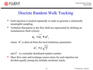
12/26/25 55 Fluent Software Training TRN-99-003 Discrete Random Walk Tracking Each injection is tracked repeatedly in order to generate a statistically meaningful sampling. Turbulent fluctuation in the flow field are represented by defining an instantaneous fluid velocity: where is derived from the local turbulence parameters: and is a normally distributed random number Mass flow rates and exchange source terms for each injection are divided equally among the multiple stochastic tracks. i i i u u u ' i u' 3 2 ' k i u
56.
© Fluent Inc.
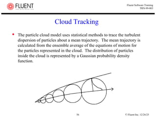
12/26/25 56 Fluent Software Training TRN-99-003 Cloud Tracking The particle cloud model uses statistical methods to trace the turbulent dispersion of particles about a mean trajectory. The mean trajectory is calculated from the ensemble average of the equations of motion for the particles represented in the cloud. The distribution of particles inside the cloud is represented by a Gaussian probability density function.
57.
© Fluent Inc.
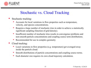
12/26/25 57 Fluent Software Training TRN-99-003 Stochastic vs. Cloud Tracking Stochastic tracking: Accounts for local variations in flow properties such as temperature, velocity, and species concentrations. Requires a large number of stochastic tries in order to achieve a statistically significant sampling (function of grid density). Insufficient number of stochastic tries results in convergence problems and non-smooth particle concentrations and coupling source term distributions. Recommended for use in complex geometry Cloud tracking: Local variations in flow properties (e.g. temperature) get averaged away inside the particle cloud. Smooth distributions of particle concentrations and coupling source terms. Each diameter size requires its own cloud trajectory calculation.
58.
© Fluent Inc.
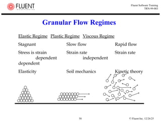
12/26/25 58 Fluent Software Training TRN-99-003 Granular Flow Regimes Elastic Regime Plastic Regime Viscous Regime Stagnant Slow flow Rapid flow Stress is strain Strain rate Strain rate dependent independent dependent Elasticity Soil mechanics Kinetic theory
59.
© Fluent Inc.
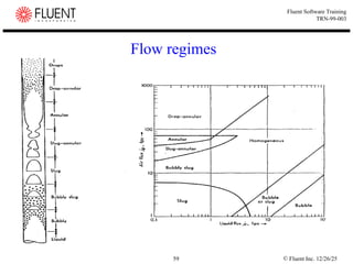
12/26/25 59 Fluent Software Training TRN-99-003 Flow regimes
60.
© Fluent Inc.
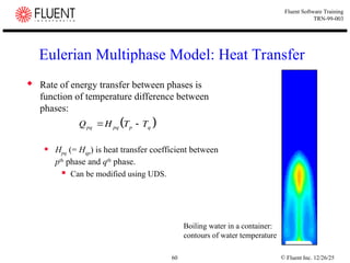
12/26/25 60 Fluent Software Training TRN-99-003 Eulerian Multiphase Model: Heat Transfer Rate of energy transfer between phases is function of temperature difference between phases: Hpq (= Hqp) is heat transfer coefficient between pth phase and qth phase. Can be modified using UDS. Q H T T pq pq p q Boiling water in a container: contours of water temperature
61.
© Fluent Inc.
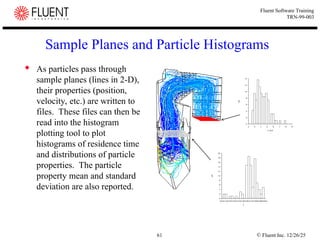
12/26/25 61 Fluent Software Training TRN-99-003 Sample Planes and Particle Histograms As particles pass through sample planes (lines in 2-D), their properties (position, velocity, etc.) are written to files. These files can then be read into the histogram plotting tool to plot histograms of residence time and distributions of particle properties. The particle property mean and standard deviation are also reported.
Download