Downloaded 532 times


![References 73
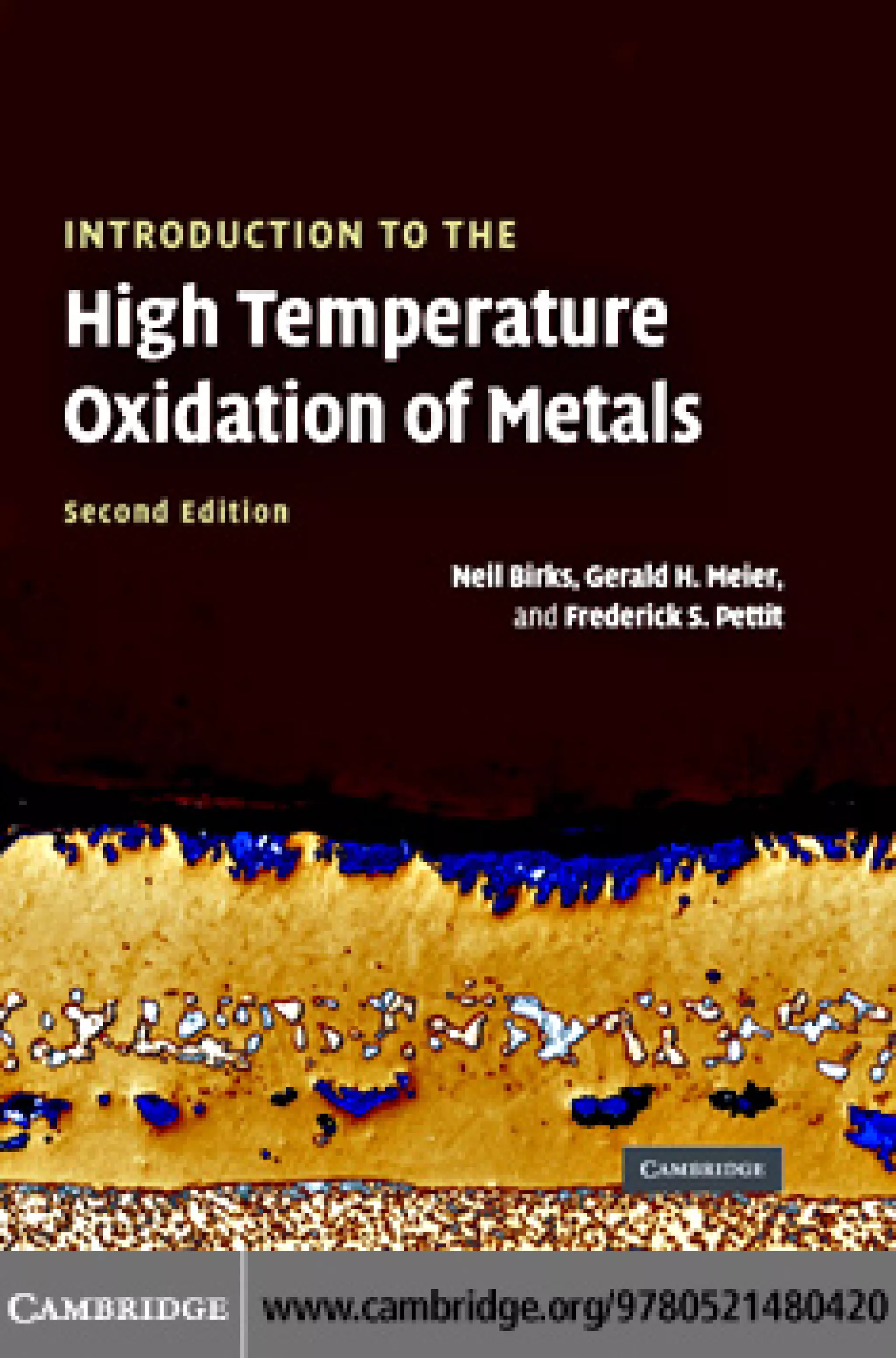
Table 3.2 Relationships between variously defined parabolic oxidation rate
constants (for the scale stoichiometry expressed as Mν X).
A k k kc kr
B cm2 s−1 g2 cm−4 s−1 cm2 s−1 equiv. cm−1 s−1
k ( cm2 s−1 ) 1 2[MX /V Z X ]2 [V M /V ]2 1/V
1 1
k (g2 cm−4 s−1 ) [V Z X ]2 /MX
2
1 [V M Z X /MX ]2 V /2[Z X /MX ]2
2 2
2
kc (cm2 s−1 ) [V /V M ]2 2[MX /V Z X ]2 1 V /V M
2
kr equiv. cm−1 s−1 V 2/V [MX /Z X ]2 V M /V 1
The relating factor F is given according to A = FB; A is listed horizontally and B vertically.
The symbols have the following meaning: V = equivalent volume of scale (cm3 equiv.−1 );
V M = equivalent volume of metal (cm3 equiv.−1 ); MX = atomic mass of non-metal X
(oxygen, sulphur, etc.); ZX = valency of X (equiv. g-atom X−1 ).
Consequently, it is necessary to check the definition of a rate constant very carefully
when evaluating quantitative data.
It is easy to calculate the value of any rate constant from any other since they all
represent the same process. The relationships are given in Table 3.2.
References
1. F. O. Kr¨ ger, The Chemistry of Imperfect Crystals, Amsterdam, North Holland
o
Publishing Co., 1964.
2. P. Kofstad, Nonstoichiometry, Diffusion, and Electrical Conductivity in Binary Metal
Oxides, New York, Wiley, 1972.
3. D. M. Smyth, The Defect Chemistry of Metal Oxides, Oxford, Oxford University
Press, 2000.
4. H. H. von Baumbach and C. Z. Wagner, Phys. Chem., 22 (1933), 199.
5. G. P. Mohanty and L. V. Azaroff, J. Chem. Phys., 35 (1961), 1268.
6. D. G. Thomas, J. Phys. Chem. Solids, 3 (1957), 229.
7. E. Scharowsky, Z. Phys., 135 (1953), 318.
8. J. W. Hoffmann and I. Lauder, Trans. Faraday Soc., 66 (1970), 2346.
9. I. Bransky and N. M. Tallan, J. Chem. Phys., 49 (1968), 1243.
10. N. G. Eror and J. B. Wagner, J. Phys. Stat. Sol., 35 (1969), 641.
11. S. P. Mitoff, J. Phys. Chem., 35 (1961), 882.
12. G. H. Meier and R. A. Rapp, Z. Phys. Chem. NF, 74 (1971), 168.
13. K. Fueki and J. B. Wagner, J. Electrochem. Soc., 112 (1965), 384.
14. C. M. Osburn and R. W. Vest, J. Phys. Solids, 32 (1971), 1331.
15. J. E. Stroud, I. Bransky, and N. M. Tallan, J. Chem. Phys., 56 (1973), 1263.
16. R. Farhi and G. Petot-Ervas, J. Phys. Chem. Solids, 39 (1978), 1169.
17. R. Farhi and G. Petot-Ervas, J. Phys. Chem. Solids, 39 (1978), 1175.](https://image.slidesharecdn.com/introductiontothehightemperatureoxidationofmetals-121106030521-phpapp02/75/Introduction-to-the_high_temperature_oxidation_of_metals-87-2048.jpg)


![82 Oxidation of pure metals
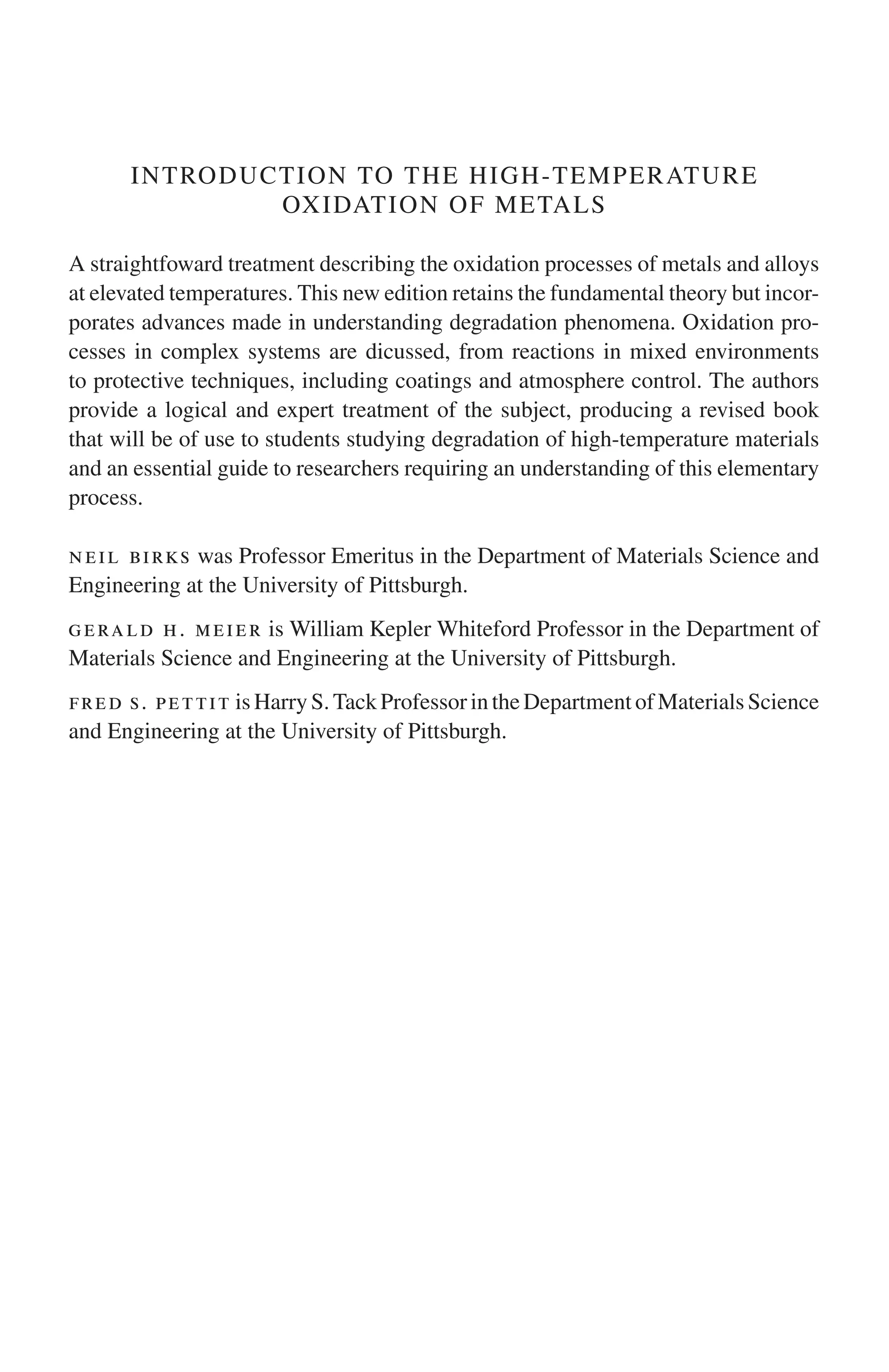
Figure 4.4 Variation of concentration of singly or doubly charged interstitial zinc
ions across a ZnO scale for high and low oxygen partial pressures.
Oxidation of aluminium
The thermodynamically stable oxide of aluminium is α-Al2 O3 . This oxide has a
rhombohedral structure consisting of a hexagonal packing of oxide anions with
cations occupying two-thirds of the octahedral interstitial sites. Alpha is a slowly-
growing oxide and is the protective film formed on many high-temperature alloys
and coatings. This will be discussed in the next chapter. Alumina also exists in
a number of metastable crystal structures.21 These include γ -Al2 O3 , which is a
cubic spinel, δ-Al2 O3 , which is tetragonal, and θ-Al2 O3 , which is monoclinic.
Another form, κ-Al2 O3 , which is similar to α but has a shift in the stacking
sequence on the anion sub-lattice, has also been identified.22 Some of the metastable
aluminas sometimes form prior to the stable α on high-temperature alloys and
predominate for the oxidation of aluminium at temperatures below its melting point
of 660 ◦ C.
At room temperature Al is always covered with an ‘air-formed film’ 2–3 nm in
thickness,23 which consists of amorphous alumina. Oxidation at temperatures less
than 350 ◦ C results in growth of the amorphous film following inverse logarithmic
kinetics.24 At temperatures between 350 and 425 ◦ C the amorphous film grows
with parabolic kinetics.24 At temperatures above 425 ◦ C the kinetics are complex.
Investigations by TEM23,24 and secondary-ion mass spectroscopy (SIMS)25 suggest
the following sequence. The pre-existing film grows initially and, following an
incubation period, γ -Al2 O3 crystals nucleate at the amorphous oxide–Al interface.
The γ nucleates heterogeneously on the surface at ridges resulting from specimen
preparation and grows by oxygen transport through local channels in the amorphous
film and anion attachment at the peripheries of the growing γ islands. The origin
of the local channels have been proposed to be cracks in the amorphous oxide over
the surface ridges.23 Oxidation of a [111]-oriented Al single crystal which was
sputter-cleaned and oxidized at 550 ◦ C resulted in direct γ nucleation without the
development of an amorphous layer.25](https://image.slidesharecdn.com/introductiontothehightemperatureoxidationofmetals-121106030521-phpapp02/75/Introduction-to-the_high_temperature_oxidation_of_metals-96-2048.jpg)


![Base parent with base-alloying elements 123
results can be obtained depending upon surface conditions. In fact, in such regions,
a given specimen may develop different oxide scales at different locations upon
its surface. This diagram indicates that NiAl should form and maintain protective
alumina under all conditions while Ni3 Al (γ ) is a ‘marginal’ alumina former at
temperatures below 1200 ◦ C.
The stable form of alumina is always the α (corundum) structure. However, under
some conditions it is preceded by metastable forms.35 The oxide scales formed on
Ni3 Al at oxygen partial pressures on the order of 1 atm in the temperature range
950–1200 ◦ C consist mainly of Ni-containing transient oxides, NiO and NiAl2 O4 ,
over a layer of columnar α-alumina. Schumann and R¨ hle36 studied the very early
u
stages of transient oxidation of the (001) faces of Ni3 Al single crystals in air at
950 ◦ C using cross-section transmission electron microscopy (TEM). After 1 min
oxidation simultaneous formation of an external NiO scale and internal oxidation of
γ were observed. The internal oxide particles were identified as γ -Al2 O3 , which
possesses a cube-on-cube orientation with respect to the Ni matrix. After 6 min
oxidation a continuous γ -Al2 O3 layer had formed between the IOZ and the γ single
crystal. Oxidation for 30 min resulted in a microstructure similar to the 6 min
oxidation but the Ni in the two-phase zone was oxidized to NiO. Oxidation for 50 h
resulted in a scale consisting of an outer layer of NiO, an intermediate layer of
NiAl2 O4 , and an inner layer of γ -Al2 O3 in which α-Al2 O3 grains had nucleated at
the alloy–oxide interface. The spinel was presumed to have formed by a solid-state
reaction between NiO and γ -Al2 O3 . A crystallographic orientation relationship was
found between the α- and γ -alumina, whereby (0001)[1100]α || [(111)[110]γ , i.e.,
¯ ¯
close-packed planes and close-packed directions of α are parallel to close-packed
planes and directions in γ .
The oxidation of NiAl is somewhat unique in that, at temperatures of 1000 ◦ C and
above, there are negligible amounts of Ni-containing transient oxides. The transient
oxides are all metastable phases of Al2 O3 (γ , δ, and/or θ).35 The transition of these
metastable phases to the stable α-Al2 O3 results in significant decreases in the scale
growth rate and a ‘ridged’ oxide morphology which is distinct from the colum-
nar morphology observed on Ni3 Al.35 The transition aluminas have been shown to
grow primarily by outward migration of cations while α-alumina grows primarily
by inward transport of oxygen along oxide grain boundaries. The effect of oxidation
time and temperature on the phases present in the scales has been studied by sev-
eral authors. Rybicki and Smialek37 identified θ-alumina as the transient oxide on
Zr-doped NiAl and found that the transition to α occurred at longer times at lower
oxidation temperatures, e.g., scales consisted entirely of θ after 100 h at 800 ◦ C
while it transformed to α in about 8 h at 1000 ◦ C. Only α was observed at 1100
and 1200 ◦ C. Pint and Hobbs38 observed only α on undoped NiAl after 160 s at
1500 ◦ C. Brumm and Grabke39 observed two transformations at 900 ◦ C for undoped
NiAl. The scale consisted initially of γ -alumina which transformed to θ-alumina](https://image.slidesharecdn.com/introductiontothehightemperatureoxidationofmetals-121106030521-phpapp02/75/Introduction-to-the_high_temperature_oxidation_of_metals-137-2048.jpg)


![Measurement of stresses 141
[hkl ]
Diffracted beam S3 Incident beam
ψ
θb θb Tilting axis
{hkl } S2
φ
S1
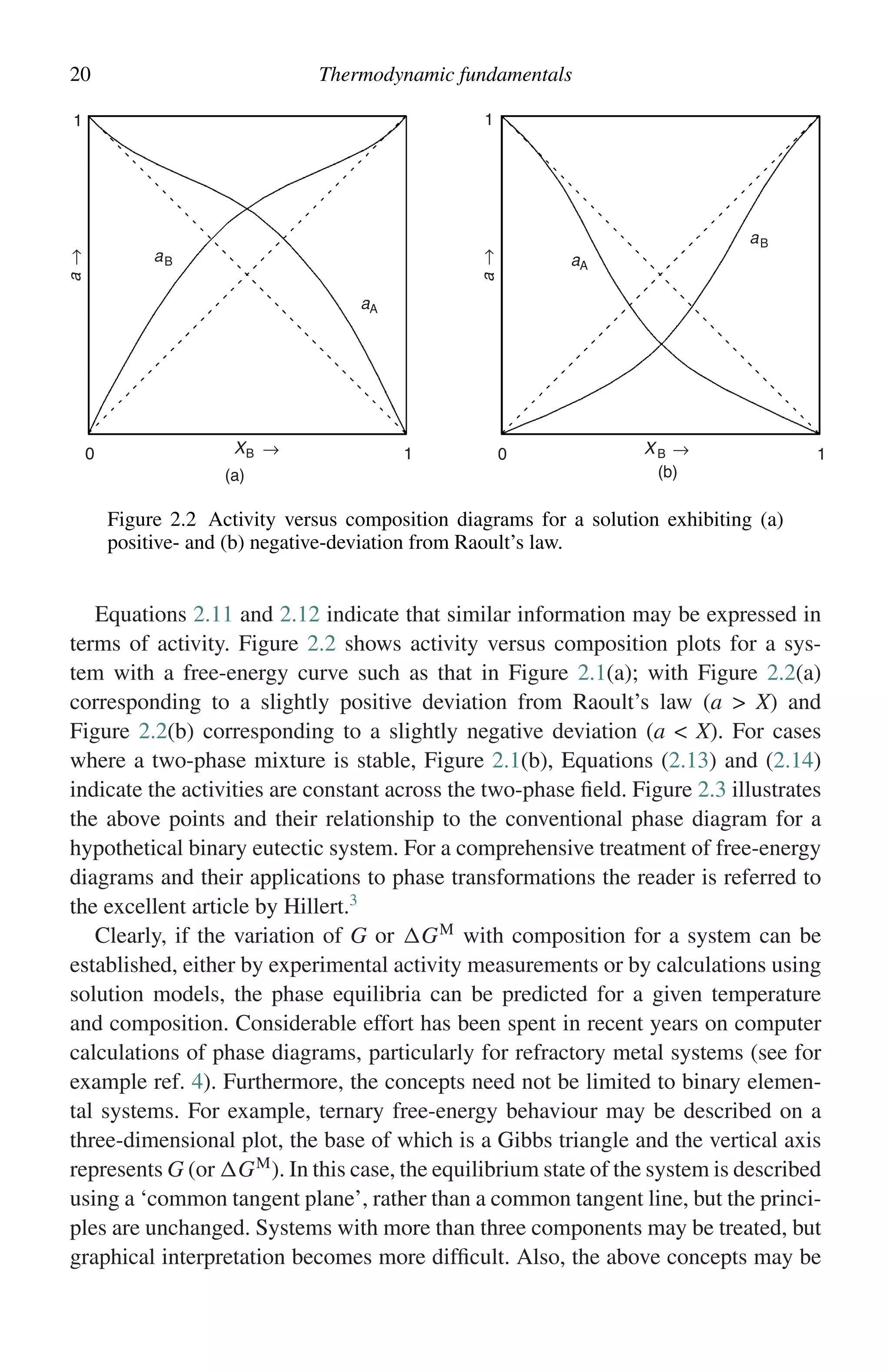
Figure 5.34 Schematic diagram of the tilting technique for measuring the strains
in an oxide layer.
X-Ray diffraction
The strain in an oxide film can be measured by X-ray diffraction (XRD) as a change
in lattice spacing with inclination, with respect to the surface of a sample. This strain
is usually expressed as in Equation (5.37),
dφψ − do
εφψ = (5.37)
do
in which do is the stress-free lattice spacing of the selected (hkl) planes and dφψ
is the lattice spacing of these (hkl) planes in the stressed-film for a given tilt ψ.
The geometry of the commonly used ‘tilting technique’ is presented in Figure 5.34.
It can be shown that this strain is expected to be proportional to sin2 ψ. For an
equal biaxial stress in the irradiated layer, Equation (5.37) can be expressed as in
Equation (5.38):83
dφψ − do 1+ν ν
= σφ sin2 ψ − (σ1 + σ2 ). (5.38)
do E E
If a plot of ε versus sin2 ψ curve is linear, as is expected from an isotropic sur-
face layer which is polycrystalline and not textured, the stress can be accurately
calculated from the slope of the d vs. sin2 ψ line and values for E, ν, and do . This
technique and variations thereof have been used to measure the stresses in alumina
films both at room temperature and during oxidation at high temperature (see, for
example, ref. 84). Growth stresses in alumina can vary from negligible values to
greater than 1 GPa compression. The residual stress, which includes the effects of
growth and thermal stresses, can exceed 5 GPa compression for oxidation temper-
atures on the order of 1100 ◦ C. The stresses generated in chromia films have been
investigated by several groups using XRD techniques. Hou and Stringer85 measured
the residual stress in chromia on Ni–25 wt% Cr–1 wt% Al and Ni–25 wt% Cr–0.2
wt% Y after oxidation at 1000 ◦ C and found the stresses to be compressive and of
similar magnitude for both alloys. Comparison with calculated thermal stresses led
to the conclusion that growth stresses were negligible. Shores and coworkers,86 on
the other hand, have reported substantial compressive growth stresses for chromia](https://image.slidesharecdn.com/introductiontothehightemperatureoxidationofmetals-121106030521-phpapp02/75/Introduction-to-the_high_temperature_oxidation_of_metals-155-2048.jpg)


![168 Oxidation in oxidants other than oxygen
Equations (6.6)–(6.8):
1/2
[VFe ] = const. pS2 , (6.6)
1/4
VFe = const. pS2 , (6.7)
1/6
VFe = const. pS2 . (6.8)
Mrowec,16 using existing data24–26 , calculated that the concentration of iron-ion
vacancies was proportional to the sulphur partial pressure to the power of 1/1.9 at
800 ◦ C. This result is consistent with the metallic nature of FeS,1 i.e., there are an
insignificant number of localized electronic defects.
One final interesting point about sulphidation is that, because the free energies
of formation of the sulphides of iron, nickel, cobalt, chromium, and aluminium are
quite similar, selective sulphidation of chromium and aluminium is not favoured
as in the case of oxidation. Lai9 has reviewed the literature of the sulphidation of
alloys and has made several generalizations as follows.
(1) Alloys of iron, nickel, and cobalt sulphidize at similar rates – within an order of mag-
nitude.
(2) Alloys containing less than 40% Cr may show improved sulphidation resistance by
forming an inner layer of ternary sulphide or chromium sulphide. It has been found
that Cr concentrations in excess of 17 wt% Cr provide some sulphidation protection in
steels.27
(3) Alloys containing more than 40% Cr could form a single, protective, outer layer of
Cr2 S3 . At the higher Cr levels, all three alloy systems showed similar resistance.
(4) The presence of Al in Fe and Co alloys could be beneficial due to the formation of an
aluminium-based sulphide. In the case of Ni-based alloys the results were erratic.
(5) However, formation of Al2 S3 scales is not particularly useful because they react with
H2 O, even at room temperature.
On the other hand, refractory-metal sulphides are both very stable and slow growing.
This has been addressed by Douglass and coworkers,28–35 who demonstrated that
the addition of Mo and Mo plus Al to nickel substantially reduced the parabolic rate
constant for sulphidation, by about five orders of magnitude for the composition
Ni–30 wt% Mo–8 wt% Al; and, in the case of iron alloys, by six orders of magnitude
for the composition Fe–30 wt% Mo– 5 wt% Al. In these cases the scales formed
were Al0.5 Mo2 S4 , which gave excellent resistance to sulphidation, but would form
molybdenum oxides in oxidizing atmospheres.13](https://image.slidesharecdn.com/introductiontothehightemperatureoxidationofmetals-121106030521-phpapp02/75/Introduction-to-the_high_temperature_oxidation_of_metals-182-2048.jpg)


This document discusses methods for investigating the high-temperature oxidation of metals. Kinetics measurements involve exposing specimens to oxidizing conditions for periods of time and then examining them. There are uncertainties in determining when oxidation begins. Common techniques to characterize reaction products include measuring mass changes, analyzing gas consumption or product formation, and examining specimen cross-sections using microscopy. Accelerated testing aims to produce representative microstructures in shorter times than actual service conditions.