Introduction to Data , Information, Meta Data

Database Management
Systems(CS23332)
II YEAR- III SEMESTER

UNIT-I
DATABASE SYSTEMS AND SQL QUERY
9
Introduction – Purpose of Database Systems - View of Data –Database Architecture -Database Schema – Keys – Codd’s Rule –RDBMS- SQL: Data Definition –
Domain types – Structure of SQL Queries - Modifications of the database –Set Operations–Aggregate Functions– Null Values- SQL Nested Sub q ueries –Complex
Queries–Views – Joined relations.
UNIT-II PL/SQL,DATAMODEL AND QUERYPROCESSING 9
PL/SQL:Functions,Procedures,Triggers,Cursors–DynamicSQL–RelationalAlgebra-TupleRelationalcalculus- Domain Relational Calculus–Entity Relationship
Model–Constraints-Entity Relationship Diagram-Design Issues of ER Model – Extended ERFeatures –Mapping ER Model to Relational Model– Query Processing –
Heuristics for Query Optimization.
UNIT-III NORMAL FORMS AND INDEXING 9
Motivation for Normal Forms – Functional dependencies – Armstrong’s Axioms for Functional Dependencies – Closure for a set of Functional Dependencies –
Definitions of 1NF-2NF-3NF and BCNF – Multi valued Dependency 4NF - Joint Dependency- 5NF-File Organization-Indexing B+ tree - B-Tree
UNIT-IV TRANSACTIONS 9
Transaction Concepts – ACID Properties – Schedules – Serializability – Transaction support in SQL – Need for Concurrency – Concurrency control –Two Phase Locking-
Timestamp – Multi version – Validation and Snapshot isolation– Multiple Granularity l ocking –Deadlock Handling–Recovery Concepts –Recovery based on deferred
and immediate update – Shadow paging – ARIES Algorithm
UNIT-V NOSQL DATABASE 9
No SQL Database vs.SQL Databases – CAP Theorem –Migrating from RDBMS to No SQL – Mongo DB – CRUD Operations– Mongo DB Sharding – MongoDB Replication
– Web Application Development using MongoDB with Python and Java.
3
SYLLABUS Credits:5

Text Book(s):
1.Abraham Silberschatz, Henry F. Korth and S. Sudharshan, “Database System Concepts”, Seventh
Edition, Mc Graw Hill, March 2019.
2.P. J. Sadalage and M. Fowler, "NoSQL Distilled: A Brief Guide to the Emerging World of Polyglot
Persistence", Addison-Wesley Professional, 2013.
Reference Books(s)/Weblinks:
1.RamezElmasriandShamkantB.Navathe,“FundamentalsofDatabaseSystems”,SeventhEdition,Pearson
Education, 2016.
2.C.J.Date,A.KannanandS.Swamynathan,“AnIntroductiontoDatabaseSystems”,EighthEdition,Pearson
Education, 2006.
3.AtulKahate,“IntroductiontoDatabaseManagementSystems”,PearsonEducation,NewDelhi,2006.
4.StevenFeuersteinwithBillPribyl,”OraclePL/SQLProgramming”,sixthedition,Publisher:O'Reill2014.
5.MongoDB:TheDefinitiveGuide,3rdEdition,byKristinaChodorow,ShannonBradshaw,Publisher:O'Reilly
Media,2019
6.ShashankTiwari,”ProfessionalNoSQL”,Wiley,2011.
7.DavidLane,Hugh.E.Williums,WebDatabaseApplicationswithPHPandMySQL,O’ReillyMedia;2nd
edition, 2004
4

Time Tuesday Wed Thur Fri
THEORY SESSIONS
9:00 - 9:50
CS23332
A102
12:00 - 12:50
CS23332
A103
3:00 - 3:50
CS23332
A102
LAB SESSIONS
8:00 - 9:40
CS23332 Batch 2
JL1
10:00 - 11:40
CS23332 Batch 1
TLFL4
1:20 - 3:00
CS23332 Batch 2
TLGL3
3:00 - 4:40
CS23332 Batch 1
KFL01
TIME TABLE

Unit 1
Introduction to Database Management Systems
8

Introduction to Data , Information,
Meta Data
Data:-Raw facts and figures that can be recorded.
Information: Meaningful (processed) data is known as information.
Meta Data: Data that describe the properties of other data is Know
as Metadata . Actually, Metadata keeps the information of other data
Example-
10,971,108
lllData
lllChennai Population in 2020
lllInformation
9

Traditional File System
10
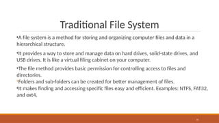
•A file system is a method for storing and organizing computer files and data in a
hierarchical structure.
•It provides a way to store and manage data on hard drives, solid-state drives, and
USB drives. It is like a virtual filing cabinet on your computer.
•The file method provides basic permission for controlling access to files and
directories.
◦Folders and sub-folders can be created for better management of files.
•It makes finding and accessing specific files easy and efficient. Examples: NTFS, FAT32,
and ext4.

File Processing System(Traditional Approach)
□ In the traditional file-based approach, many organization
exclusively used file processing systems to store and
manage data.
□ In this file processing system, each unit or department in
an organization has its own set of separate files
and the records are grouped based on their categories. The
data in one file may not relate to the data in any other
file.
11

File Processing Data Weakness
12
Data redundancy- Data redundancy occur when the same data items are stored in multiple
files due to each unit or department in an organization has its own sperate files in the file
processing system.
For example, the Student contract file and the Student file store the same students’ names
and addresses.
Wastes resources- Duplicating data in this way is a waste of storage space and people’s time.
This is because file maintenance tasks require people to spend time in updating or deleting
multiple files that contain the same data whenever the data is modified. It also Increases the
chance of errors. If a student changes his or her telephone numbers,
for example, the school must update the student contract file. If no change is made in all the
files where the data stored, then inconsistencies among the files exist.

File Processing Data Weakness(Contd.)
13
Isolated Data – Isolated data increase the difficulty in accessing the data that stored in
separate files in different departments.
For example, to send an email to a teacher regarding the student's academic program
progress, data is needed from both the Student name file and Student performance file.
Sharing data from multiple and separate files is a complicated procedure especially when
there are many files involved.

Introduction to Database Approach
14

Definition: Database, Database system
Database:
It is a collection of interrelated data. These can be stored in the form of
tables.
A database can be of any size and varying complexity.
A database may be generated and manipulated manually or it may be
computerized.
Example: Customer database consists the fields as cname, cno, and ccity
15

Definition: Database Management system
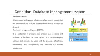
Database System:
It is computerized system, whose overall purpose is to maintain
the information and to make that the information is available on
demand
Database Management System (DBMS):
It is a collection of programs that enables user to create and
maintain a database. In other words, it is general-purpose
software that provides the users with the processes of defining,
constructing and manipulating the database for various
applications.
16

Purpose of Data base System
17
Reduced Data Redundancy – Most data or records are stored in only one file, which will
greatly reduce duplicate data that might lead to confusion and mishandling.
Improved Data Integrity – When users modify data in the database, they can directly make
changes to one file instead of multiple files. Therefore, the mismatch in different copies of
same data will not occur. This database approach increases the quality and data’s integrity
by reducing the possibility of causing inconsistencies.
Shared Data – The data in a database is shared among by multiple users who have access to
the system. Organizations that use databases typically have security settings to define who
can access, add, modify, and delete the data in a database.

Purpose of Data Base System
18
Easier Access – The database approach allows nontechnical users to access, maintain and
even develop smaller database without professional assistance.
Reduced Development Time – It often is easier and faster to develop programs that use the
database approach.

Difference between File System and
DBMS
19

Views of Data
DATA ABSTRACTION
Hide irrelevant data
Provide an abstract view of the data.
Developers hide irrelevant data from the user and
provide them the relevant data.
Based on this system will also work efficiently.
In DBMS, data abstraction is performed in layers
which means there are levels of data abstraction
20

Views of Data
21
“Schema” and “Instance” are key ideas in a database management system (DBMS) that help organize
and manage data.
Instances
An Instance is the state of an operational database with data at any given time.
It contains a snapshot of the database. The instances can be changed by certain CRUD operations,
such as like addition, and deletion of data.
It may be noted that any search query will not make any kind of changes in the instances.
Example:
Let’s say a table teacher in our database whose name is School, suppose the table has 50 records so
the instance of the database has 50 records for now and tomorrow we are going to add another fifty
records so tomorrow the instance has a total of 100 records. This is called an instance

Views of Data
Schema
Schema is the overall description of the database. The basic
structure of how the data will be stored in the database is
called schema.
Schema is of three types: Logical Schema, Physical Schema
and view Schema.
Physical Schema – It describes the database designed at the
physical level.
Logical Schema – It describes the database designed at a
logical level.
View Schema – It defines the design of the database at the
view level.
22

Views of Data
23
Example:
Let’s say a table teacher in our database named school, the teacher table requires the name,
dob, and doj in their table so we design a structure as:
Teacher table name: String doj: date dob: date

DATA BASE SYSTEM ARCHITECTURE
24
i) Data files: Used for storing database itself.
ii) Data dictionary: Used for storing metadata, particularly
schema of database.
iii) Indices: Indices are used to provide fast access to data
items present in the database

Data Base system Architecture
25
The two important components of database architecture are - Query processor and storage manager.
Query processor:
The interactive query processor helps the database system to simplify and facilitate access to data. It
consists of DDL interpreter, DML compiler and query evaluation engine.
With the following components of query processor, various functionalities are performed -
i)DDL interpreter: This is basically a translator which interprets the DDL statements in data
dictionaries.
ii)DML compiler: It translates DML statements query language into an evaluation plan. This plan
consists of the instructions which query evaluation engine understands.
iii)Query evaluation engine: It executes the low-level instructions generated by the DML compiler.

26
Storage manager:
Component of database system that provides interface between the low level data stored in the database
and the application programs and queries submitted to the system.
Responsible for storing, retrieving, and updating data in the database. The storage manager components
include -
i)Authorization and integrity manager:
Validates the users who want to access the data and tests for integrity constraints.
ii)Transaction manager: Ensures that the database remains in consistent despite of system failures and
concurrent transaction execution proceeds without conflicting.
iii)File manager: Manages allocation of space on disk storage and representation of the information on disk.
iv)Buffer manager: Manages the fetching of data from disk storage into main memory. The buffer manager
also decides what data to cache in main memory. Buffer manager is a crucial part of database system.

27
Storage manager implements several data structures such as -
i)Data files: Used for storing database itself.
ii)Data dictionary: Used for storing metadata, particularly schema of database.
iii)Indices: Indices are used to provide fast access to data items present in the database
IV)Statistical data includes various metrics or statistics about the database objects, such as
tables, columns, and indexes, It typically consists of:
•Number of rows in a table
•Number of distinct values in a column
•Minimum and maximum values in a column
•Data distribution (histograms)
•Null values count
•Index cardinality (number of unique values in an index)

Database Users
28
•There are four different types of database-system users, differentiated by the way they expect to
interact with the system.
• Different types of user interfaces have been designed for the different types of users.
•Naive users: Naive users interact with the system by invoking one of the application programs
that have been written previously.
• Naive users are typical users of form interface, where the user can fill in appropriate fields of the form.
• Naive users may also simply read reports generated from the database
•Application programmers Application programmers are computer professionals who write
application programs. Application programmers can choose from many tools to develop user
interfaces.

Database Users(Cont.)
29
•Sophisticated users: Sophisticated users interact with the system without writing programs.
Instead, they form their requests in a database query language.
• They submit each such query to a query processor that the storage manager understands.
• Online analytical processing (OLAP) tools simplify analysis and data mining tools specify certain kinds of
patterns in data
•Specialized users: Specialized users are sophisticated users who write specialized database
applications that do not fit into the traditional data-processing framework.
• The applications are computer-aided design systems, knowledge base and expert systems, systems that
store data with complex data types .

Database Administrator
30
•A person who has central control over the system is called a database administrator (DBA).
Functions of a DBA include:
• Schema definition
• Storage structure and access-method definition
• Schema and physical-organization modification
• Granting of authorization for data access
• Routine maintenance
• Periodically backing up the database
• Ensuring that enough free disk space is available for normal operations, and upgrading disk space as
required
• Monitoring jobs running on the database

History of SQL
31
IBM Sequel language developed as part of System R project at the IBM San Jose Research
Laboratory
Renamed Structured Query Language (SQL) ANSI and ISO standard SQL:
◦SQL-86
◦SQL-89
◦SQL-92
◦SQL:1999 (language name became Y2K compliant!)
◦SQL:2003
◦SQL 2023 JSON (java script object notation) support
Commercial systems offer most, if not all, SQL-92 features, plus varying feature sets from
later standards and special proprietary features.
◦Not all examples here may work on your particular system.

Domain Types in SQL
32
char(n). Fixed length character string, with user-specified length n.
varchar(n). Variable length character strings, with user-specified maximum length n.
int. Integer (a finite subset of the integers that is machine-dependent).
Date. Stores date value in yyyy-mm-dd format.ex 2025-07-23
Time. Stores time values in hh-mm-ss format.ex 14:30:00
Timestamp. Both date and time together. Ex:'2025-07-23 14:30:00'
Decimal/numeric(p,d). Fixed point number, with user-specified precision of p digits, with n
digits to the right of decimal point.
float(n). Floating point number, with user-specified precision of at least n digits.
Boolean. Store True or False
BLOB. Stores binary large object. Ie image files

Keys in DBMS
s.
Types of keys:
Primary key : Uniquely identifies each record in a table. Cannot be Null.
Candidate key: Alternative unique keys that could be primary key
Super Key: Combination of attributes that uniquely identify record(Ex:
[regno, aadharno},{regno,dob})
Composite key: Combined attributes used as a single key (ex:{name,dob})
Foreign key: Establishes a relationship between tables.
Unique Key: Ensures column(s) have unique values.
Surrogate Key: Artificial keys assigned for record identification.
34

Primary key example
1.Primary Key
uniquely identifies all the records within that table
Properties of a Primary Key
The Primary Key field shouldn’t be left NULL; the
Primary Key column must contain a value.
In that column, no two rows in the table
may contain identical values.
If a foreign key in a DBMS refers to the
primary Key, no value may be altered or modified in this
primary key
36

Keys in DBMS
2.Foreign key
A foreign key is generally a primary key from one
table that appears as a field in another
where the first table has a relationship to the second.
In other words, if we had a table A with a primary key
X that linked to a table B where
X was a field in B, then X would be a foreign key in B.
37

Keys in DBMS
3.Composite Keys:
A composite key in SQL is a combination of
two or more columns that is used to identify a
row in a table uniquely.
It is an alternative to using a single-column
primary key, and it is often used when a single
column is not sufficient to identify a row
uniquely.
38

Keys in DBMS
4.Candidate keys
A set of attributes that uniquely
identify each tuple within a table.
39

Keys in DBMS
5.Super keys
Super keys in DBMS are collections of
properties that uniquely identify tuples in
a relational database table.
For the purpose of creating and managing
dependable and effective databases, it is
essential to comprehend super keys.
40

Keys in DBMS
6.Surrogate Key
A Surrogate Key is just a unique identifier
for each row and it may use as a
Primary Key.
A Surrogate Key is also known as an
artificial key or identity key.
It can be used in data warehouses.
This type of key is either database
generated or generated via
another application (not supplied by user).
41

Difference between keys in DBMS
42
Key Type Definition Uniqueness Null Values Purpose Index Usage Alteration
Primary Key
Uniquely
identifies each
record in a
table.
Required Not Allowed
Data integrity,
record
identification.
Creates Unique
Index
Within same
table
May be
complex,
impact other
tables.
Foreign Key
Establishes a
relationship
between
tables.
Not Required Allowed
Data
consistency,
relationship
maintenance.
May create
Index
Between tables
More flexible
for
maintenance.
Candidate Key
Alternative
unique keys
that could be
primary keys.
Backup
primary key
options.
May create
Index
Within same
table
May become
primary key.

Difference between keys in DBMS
43
Key Type Definition Uniqueness Null Values Purpose Index Usage Alteration
Composite Key
Combined
attributes used
as a single key. Required Not Allowed
Specialized
unique
identification.
Creates
Composite
Index
Within same
table
May be
complex,
impact
performance.
Unique Key
Ensures
column(s) have
unique values. Required Allowed
Enforce
uniqueness, no
primary key.
Creates Unique
Index
Within same
table
May be used as
primary key.
Surrogate Key
Artificial keys
assigned for
record
identification.
Enhanced data
privacy, data
warehousing.
Creates Unique
Index
Within same
table
Generally static,
non-changing.

OVERVIEW OF CODD’s RULE
44
•Any database which simply has relational data model is not a relational database system
(RDBMS).
•There are certain rules for a database to be perfect RDBMS. These rules are developed by Dr.
Edgar F Codd in 1985 to define a perfect RDBMS. For a RDBMS to be a perfect RDBMS, it must
follow his rules.
•EF Codd has developed 13 rules for a database to be a RDBMS.
•According to him, all these rule help to have perfect RDBMS and hence correct data and relation
among the objects in database.
•But none of the database follows all these rules; but obeys to some extent.
•For example, Oracle supports 11.5 of E.F. CODD Rule. The .5 missing was according to E.F. CODD
Rule DML operation through a complex view is possible. But in oracle DML operation through a
complex view is not always.

CODD’s Rules
Rule No
0
Rule Name
Foundational Rule
Application to Online Shopping System
Database system should be relational in nature and must have a
management system
1 Information Rule All data is stored in tables (relations).
2 Guaranteed Access Rule
Each data item is accessible via table name, column name, and primary
key.
3 Systematic Treatment of NULL
NULLs used for missing/unknown values (e.g., shipping date if not
shipped).
4 Dynamic Online Catalog Metadata (table, columns) stored in relational format and can be queried.
5 Comprehensive Data Sub-language Use of SQL for all data access.
6 View Updating Rule Views (e.g., user orders) are updatable.
7 High-Level Insert, Update, Delete Use of SQL to perform set operations (insert, update, delete).
8 Physical Data Independence Queries work even if physical storage changes.
9 Logical Data Independence Schema changes (adding columns) don’t break existing queries.
10 Integrity Independence Constraints defined in schema, not in application code.
11 Distribution Independence Works across distributed databases.
12 Non-subversion Rule If using lower-level access, cannot bypass relational rules.

Codd’s Rule 0
46
▪This is the foundational Rule.
▪This rule states that any database system should be relational in nature and must have a
management system to be RDBMS.
▪That means a database should be a relational by having the relation / mapping among the tables
in the database. They have to be related to one another by means of constraints/ relation. There
should not be any independent tables hanging in the database.
▪RDBMS is management system – that means it should be able to manage the data, relation,
retrieval, update, delete, permission on the objects. It should be able handle all these
administrative tasks without affecting the objectives of database. It should be performing all
these tasks by using query languages.

Codd’s Rule 1
47
▪Information Rule
All information in the database is to be represented in one and only one way. Data must be stored in a table in
the form of rows and columns.
The order of rows and columns in the table should not affect the meaning of the table. Each cell should have
single data.
There should not be any group/range of values separated by comma, space or hyphen (Normalized data).
▪This rule is satisfied by all the databases.
For example:
Order of storing personal details about ‘Ram’ and ‘Hari’ in PERSON table should not have any difference. There
should be flexibility of storing them in any order in a row. Similarly, storing Person name first and then his
address should be same as storing address and then his name. It does not make any difference on the meaning
of table.

Codd’s Rule 2
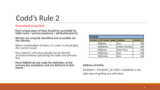
Guaranteed access Rule.
▪Each unique piece of data should be accessible by,
table name + primary key(row) + attribute(column).
▪All data are uniquely identified and accessible via
this identity.
▪When combination of these 3 is used, it should give
the correct result.
▪Any column/ cell value should not be directly
accessed without specifying the table and primary
key.
▪Most RDBMS do not make the definition of the
primary key mandatory and are deficient to that
extent .
Address of Kathy
STUDENT + STUDENT_ID (100) + ADDRESS is the
right way of getting any cell value.
48

Codd’s Rule 3
Systematic Treatment of NULL
▪This rule states about handling the NULLs in
the database.
▪As database consists of various types of data,
each cell will have different datatypes. If any
of the cell value is unknown, or not applicable
or missing, it cannot be represented as zero or
empty.
▪It will be always represented as NULL. This
NULL should be acting irrespective of the
datatype used for the cell. When used in
logical or arithmetical operation, it should
result the value correctly.
49

Codd’s Rule 4
50
Active Online Catalog
▪This rule illustrates data dictionary.
▪Metadata should be maintained for all the
data in the database.
▪These metadata stored in the data dictionary
should also obey all the characteristics of a
database.
▪We should be able to access these metadata
by using same query language that we use to
access the database.
Example:
▪SELECT * FROM ALL_TAB;
ALL_TAB is the table which has the table
definitions that the user owns and has access.

Codd’s Rule 5
51
Comprehensive Data Sub-Language Rule
▪Any RDBMS database should not be directly
accessed.
▪It should always be accessed by using some
strong query language.
▪This query language should be able to access
the data, manipulate the data and maintain
the consistency , atomicity ,and integrity of the
database.
Example:
▪SQL
is
a
support
structured query
language which creating
tables /
views/
constraints/indexes, accessing the records of
tables/views (SELECT),
manipulating the
records
security
by insert/delete/
update, provides by
giving differentlevel of
access
rights (GRANT and REVOKE) and integrity and
consistency by using constraints.

Codd’s Rule 6
52
View Updating Rule
▪Views are the virtual tables created by using
queries to show the partial view of the table.
▪That is views are subset of table, it is only
partial table with few rows and columns.
▪This rule states that views are also be able to
get updated as we do with its table.
Example:
▪If a view is formed as join of 3 tables, changes
to view should be reflected in base tables.

Codd’s Rule 7
53
High-level insert, update, and delete
▪This rule states that insert, update, and delete
operations should be supported for any
retrievable set rather than just for a single row
in a single table.
▪It also perform the operation on multiple row
simultaneously .
▪There must be delete, updating and insertion
at each level of operation. Set operation like
union, all union , insertion and minus should
also support.
Example:
▪Suppose employees got 5% hike in a year.
Then their salary has to be updated to reflect
the new salary. Since this is the annual hike
given to the employees, this increment is
applicable for all the employees. Hence, the
query should not be written for updating the
salary one by one for thousands of employee.
A single query should be strong enough to
update the entire employee’s salary at a time.

Codd’s Rule 8
54
Physical Data Independence
▪The ability to change the physical schema
without changing the logical schema is called
physical data independence.
▪This is saying that users shouldn’t be
concerned about how the data is stored or
how it’s accessed. In fact, users of the data
need only be able to get the basic definition of
the data they need.
EXAMPLE:
▪A change to the internal schema, such as using
different file organization or storage
structures, storage devices, or indexing
strategy, should be possible without having to
change the conceptual or external schemas.

Codd’s Rule 9
55
Logical Data Independence
The ability to change the logical (conceptual)
schema without changing the External
schema (User View) is called logical data
independence.
EXAMPLE:
The addition or removal of new entities,
attributes, or relationships to the conceptual
schema should be possible without having to
change existing external schemas or having to
rewrite existing application programs.

Codd’s Rule 10
56
Integrity Independence
Database should apply integrity rules by using
its query languages.
It should not be dependent on any external
factor or application to maintain the integrity.
The keys and constraints in the database
should be strong enough to handle the
integrity.
A good RDBMS should be independent of the
frontend application. It should at least support
primary key and foreign key integrity
constraints.
Example:
Suppose we want to insert an employee for
department 50 using an application.
But department 50 does not exists in the
system.
In such case, the application should not
perform the task of fetching if department 50
exists, if not insert the department and then
inserting the employee.
It should all handled by the database.

Codd’s Rule 11
57
Distribution Independence
▪The database can be located at the user server or at any other network.
▪The end user should not be able to know about the database servers.
▪He should be able to get the records as if he is pulling the records locally.
▪Even if the database is located in different servers, the accessibility time should be
comparatively less.

Codd’s Rule 12
58
Non-Subversion Rule
When a query is fired in the database, it will be
converted into low level language so that it can be
understood by the underlying systems to retrieve
the data.
In such case, when accessing or manipulating the
records at low level language, there should not be
any loopholes that alter the integrity of the
database.
If low level access is allowed to a system, it should
not be able to subvert or bypass integrity rules to
change the data.
This can be achieved by some sort of looking or
encryption.
Example:
Update Student’s address query should always be
converted into low level language which updates
the address record in the student file in the
memory.
It should not be updating any other record in the
file nor inserting some malicious record into the
file/memory.

Database Languages
• Database languages are specialized sets of commands and instructions used to define,
manipulate and control data within a database.
• Each language type plays a distinct role in database management, ensuring efficient storage,
retrieval and security of data.

1. Data Definition Language (DDL)
DDL is the short name for Data Definition Language, which deals with database schemas and
descriptions, of how the data should reside in the database.
•CREATE: to create a database and its objects like (table, index, views, stored procedure,
function and triggers)
•ALTER: alters the structure of the existing database
•DROP: delete objects from the database
•TRUNCATE: remove all records from a table, including all spaces allocated for the records
are removed
•COMMENT: add comments to the data dictionary
•RENAME: rename i.e change the name of an object

2. Data Manipulation Language (DML)
DML focuses on manipulating the data stored in the database, enabling users to retrieve, add, update and delete
data.
•SELECT: retrieve or display data from a database
•INSERT: insert or add data into a table
•UPDATE: updates existing data within a table
•DELETE: Delete all records from a database table
•MERGE: UPSERT operation (insert or update) i.e insert if not exists, or else update.
•CALL: call a PL/SQL or Java subprogram
•EXPLAIN PLAN: interpretation of the data access path. i.e display the execution plan that the database optimizer will use to run a given SQL
query.It shows how the database will execute the query internally.
•LOCK TABLE: concurrency Control

3. Data Control Language (DCL)
DCL commands manage access permissions, ensuring data security by controlling who can
perform certain actions on the database.
•GRANT: Provides specific privileges to a user (e.g., SELECT, INSERT).
•REVOKE: Removes previously granted permissions from a user.

4. Transaction Control Language (TCL)
TCL commands oversee transactional data to maintain consistency, reliability and atomicity.
•ROLLBACK: Undo changes made during a transaction.
•COMMIT: Saves all changes made during a transaction.
•SAVEPOINT: Sets a point within a transaction to which one can later roll back.

5. Data Query Language (DQL)
DQL is a subset of DML, specifically focused on data retrieval.
•SELECT: The primary DQL command, used to query data from the database without
altering its structure or contents.

Data Definition Language
67
Allows the specification of not only a set of relations but also information about
each relation, including:
● The schema for each relation.
● The domain of values associated with each attribute. Integrity constraints.
● The set of indices to be maintained for each relations. (ex:Create Index etc)
● Security and authorization information for each relation.
Ex:
GRANT SELECT, INSERT ON employees TO hr_staff;
REVOKE INSERT ON employees FROM hr_staff;
The physical storage structure of each relation on disk.

Create Table Construct
68
An SQL relation is defined using the create table command:
create table r (A1 D1, A2 D2, ..., An Dn,
(integrity-constraint1),
...,
(integrity-constraintk))
◦r is the name of the relation
◦each Ai is an attribute name in the schema of relation r
◦Di is the data type of values in the domain of attribute Ai
Example:
create table branch
(branch_name char(15) not null,
branch_city char(30),
assets integer);

Create: Example
CREATE TABLE EMPLOYEE (
Employee_id NUMBER(6) NOT NULL,
First_Name VARCHAR2(20),
Last_Name VARCHAR2(25) NOT NULL,
Email VARCHAR2(25) NOT NULL,
Phone_Number VARCHAR2(20),
Hire_date DATE NOT NULL,
Job_id VARCHAR2(10) NOT NULL,
Salary NUMBER(8,2),
Commission_pct NUMBER(2,2),
Manager_id NUMBER(6),
Department_id NUMBER(4) );
NAME NULL? TYPE
Employee_id Not null Number(6)
First_Name Varchar(20)
Last_Name Not null Varchar(25)
Email Not null Varchar(25)
Phone_Number Varchar(20)
Hire_date Not null Date
Job_id Not null Varchar(10)
Salary Number(8,2)
Commission_pct Number(2,2)
Manager_id Number(6)
Department_id Number(4)

Integrity Constraints in Create Table
70
primary key (column),not null ,FOREIGN KEY, CHECK, UNIQUE
Example: Declare branch_name as the primary key for branch and ensure that the values
of assets are non-negative.
create table branch (branch_name char(15) not null,
branch_city
assets
char(30),
Number CHECK (assets >= 0),
primary key (branch_name));
primary key declaration on an attribute automatically ensures not null
Ex2: ALTER TABLE DEPT ADD CONSTRAINT my_dept_id_pk PRIMARY KEY (ID);
Ex3: ALTER TABLE EMPADD CONSTRAINT emp_commission CHECK (COMMISSION > 0);
CREATE TABLE branch (
branch_name VARCHAR2(100) PRIMARY KEY,
assets NUMBER CHECK (assets >= 0)
);

constraints-example
consider two tables below
Emp(emp_id, emp_name, job_id, salary)
Department(id, name, location)
ALTER TABLE EMPADD DEPT_ID NUMBER;--- will become Emp(emp_id, emp_name, job_id, salary,DEPT_ID)
ALTER TABLE EMP
ADD CONSTRAINT my_emp_dept_id_fk
FOREIGN KEY (DEPT_ID)
REFERENCES DEPT(ID);
SELECT DISTINCT job_id FROM employees;
ALTER TABLE users
ADD CONSTRAINT unique_username UNIQUE (username);
• DISTINCT Used in SELECT(DML) to get unique rows
• UNIQUE Used in DDL (CREATE TABLE, ALTER TABLE)

Drop and Alter Table Constructs
72
The drop table command deletes all information about the dropped relation from the
database.
The alter table command is used to add ,modify ,drop attributes to an existing relation:
● alter table r add A number;
where A is the name of the attribute to be added to relation r and D is the domain of A.
The alter table command is used to Modify attribute types
● alter table r modify (A VARCHAR2(50));
The alter table command can also be used to drop attributes of a relation:
● alter table r drop A
where A is the name of an attribute of relation r

Example-Rename,ALTER and DROP
Rename the EMPLOYEES2 table as EMP.
RENAME EMPLOYEES2 TO EMP;
Drop the EMP table.
DROP TABLE EMP;
ADD the First_name column to the EMP table
ALTER TABLE EMPADD First_name varchar2(30);
Drop the First_name column from the EMP table and confirm it.
ALTER TABLE EMP DROP COLUMN First_name;
Modify the EMP table to allow for longer employee last names.(Hint: Increase the size to 50)
ALTER TABLE EMP MODIFY LAST_NAME VARCHAR2(50)

Basic DML Query Structure
74
SQL is based on set and relational operations with certain modifications and enhancements
A typical SQL query has the form:
select A1, A2, ..., An
from r1, r2, ..., rm
where P
◦Ai represents an attribute
◦ Ri represents a relation
◦ P is a predicate.
The result of an SQL query is a relation.

The select Clause
75
The select clause list the attributes desired in the result of a query
Example: find the names of all branches in the loan relation:
select distinct branch_name
from loan;

The select Clause
76
The select clause list the attributes desired in the result of a query
SQL allows duplicates in relations as well as in query results.
Example: find the names of all branches in the loan relation:
select branch_name
from loan;
To force the elimination of duplicates, insert the keyword distinct after select.
Find the names of all branches in the loan relations, and remove duplicates
select distinct branch_name
from loan;
The keyword all specifies that duplicates not be removed.
select all branch_name
from loan;

The select Clause
77
An asterisk in the select clause denotes “all attributes”
select *
from loan
The select clause can contain arithmetic expressions involving the operation, +, –, , and /,
and operating on constants or attributes of tuples.
The query:
select loan_number, branch_name, amount * 100
from loan;
would return a relation that is the same as the loan relation, except that the value of the
attribute amount is multiplied by 100.

The where Clause
78
The where clause specifies conditions that the result must satisfy
◦Corresponds to the selection predicate of the relational algebra.
To find all loan number for loans made at the Perryridge branch with loan amounts greater
than $1200.
select loan_number
from loan
where branch_name = ‘ Perryridge’ and amount > 1200
Comparison results can be combined using the logical connectives and, or, and not.
Comparisons can be applied to results of arithmetic expressions.

The where Clause (Cont.)
79
SQL includes a between comparison operator
Example: Find the loan number of those loans with loan amounts between $90,000 and
$100,000 (that is, □ $90,000 and □ $100,000)
select loan_number
from loan
where amount between 90000 and 100000;

The from Clause
80
The from clause lists the relations involved in the query
◦Corresponds to the Cartesian product operation of the relational algebra.
Find the Cartesian product borrower X loan
select *
from borrower, loan;
Find the name, loan number and loan amount of all customers having
a loan at the Perryridge branch.
select customer_name, borrower.loan_number, amount
from borrower, loan
where borrower.loan_number = loan.loan_number and
branch_name = ‘Perryridge’;

The Rename Operation
81
The SQL allows renaming relations and attributes using the as clause:
old-name as new-name
Find the name, loan number and loan amount of all customers; rename the column
name
loan_number as loan_id.
select customer_name, borrower.loan_number as loan_id, amount
from borrower, loan
where borrower.loan_number = loan.loan_number

Tuple Variables
82
Tuple variables are aliases or names assigned to rows (tuples) of a table.
Tuple variables are defined in the from clause via the use of the as clause.
Find the customer names and their loan numbers for all customers having a loan at some
branch.
select customer_name, T.loan_number, S.amount
from borrower as T, loan as S
where T.loan_number = S.loan_number
Find the names of all branches that have greater assets than some branch located in
Brooklyn.
select distinct T.branch_name
from branch as T, branch as S
where T.assets > S.assets and S.branch_city = ‘ Brooklyn’

String Operations
84
SQL includes a string-matching operator for comparisons on character strings. The operator “like”
uses patterns that are described using two special characters:
◦percent (%). The % character matches any substring.
◦underscore (_). The _ character matches any character.
Find the names of all customers whose street includes the substring “Main”.
select customer_name
from customer
where customer_street like ‘%Main%’
Match the name “Main%”
like ‘Main%’ escape ‘’
SQL supports a variety of string operations such as
◦concatenation (using “||”)
◦converting from upper to lower case (and vice versa)
◦finding string length, extracting substrings, etc.

Ordering the Display of Tuples
85
List in alphabetic order the names of all customers having a loan in Perryridge branch
select distinct customer_name
from borrower, loan
where borrower loan_number = loan.loan_number and
branch_name = ‘Perryridge’
order by customer_name asc;
We may specify desc for descending order or asc for ascending order, for each attribute;
ascending order is the default.
◦Example: order by customer_name desc

Duplicates
86
In relations with duplicates, SQL can define how many copies of tuples appear in the result.
query with duplicates rows
SELECT product, quantity
FROM orders;
query with removing duplicates rows
SELECT DISTINCT product, quantity
FROM orders;

Duplicates (Cont.)
SQL duplicate semantics:
select A1,, A2, ..., An
from r1, r2, ..., r m
where P
87

Modification of the Database – Deletion
88
Delete all account tuples at the Perryridge branch
delete from account
where branch_name = ‘Perryridge’
Delete all accounts at every branch located in the city ‘Needham’.
delete from account
where branch_name in (select branch_name
from branch
where branch_city = ‘Needham’)

Example Query
89
Delete the record of all accounts with balances below the average at the bank.
delete from account
where balance < (select avg (balance )
from account )
●Problem: as we delete tuples from deposit, the average balance changes
●Solution used in SQL:
1. First, compute avg balance and find all tuples to delete
2. Next, delete all tuples found above (without recomputing avg or retesting the
tuples)

Modification of the Database –
Insertion
90
Add a new tuple to account
insert into account
values (‘A-9732’, ‘Perryridge’,1200)
or equivalently
insert into account (branch_name, balance, account_number)
values (‘Perryridge’, 1200, ‘A-9732’)
Add a new tuple to account with balance set to null
insert into account
values (‘A-777’,‘Perryridge’, null )

Modification of the Database –
Insertion
91
Provide as a gift for all loan customers of the Perryridge branch, a $200 savings account. Let the loan
number serve as the account number for the new savings account
insert into account
select loan_number, branch_name, 200
from loan
insert into depositor
select customer_name, loan_number
from loan, borrower
where branch_name = ‘ Perryridge’
and loan.account_number = borrower.account_number
The select from where statement is evaluated fully before any of its results are inserted into the
relation (otherwise queries like
insert into table1 select * from table1 would cause problems)

Modification of the Database – Updates
92
Increase all accounts with balances over $10,000 by 6%, all other accounts receive 5%.
◦Write two update statements:
update account
set balance = balance * 1.06
where balance > 10000
update account
set balance = balance * 1.05
where balance ≤ 10000
◦The order is important

Case Statement for Conditional Updates
93
Same query as before: Increase all accounts with balances over $10,000 by 6%, all
other accounts receive 5%.
update account
set balance = case
when balance <= 10000 then balance *1.05
else balance * 1.06
end

Set Operations
94
The set operations union, intersect, and except operate on relations and correspond to the
relational algebra operations ∪, ∩, −.
Each of the above operations automatically eliminates duplicates; to retain all duplicates use
the corresponding multiset versions union all, intersect all and except all.
Suppose a tuple occurs m times in r and n times in s, then, it occurs:
◦m + n times in r union all s
◦min(m,n) times in r intersect all s
◦max(0, m – n) times in r except all s

Set Operations
95
Find all customers who have a loan, an account, or both:
(select customer_name from depositor)
union
(select customer_name from borrower)
Find all customers who have both a loan and an account
intersect
Find all customers who have an account but no loan.
except

Aggregate Functions
96
These functions operate on the multiset of values of a column of a relation, and return a
value
avg: average value min: minimum value max: maximum value sum: sum of values
count: number of values

Aggregate Functions (Cont.)
97
Find the average account balance at the Perryridge branch.
select avg (balance)
from account
Find the number of tuples in the customer relation.
select count (*)
from customer
Find the number of depositors in the bank
select count (distinct customer_name)
from depositor

Aggregate Functions – Group By
98
Find the number of depositors for each branch.
select branch_name, count (distinct customer_name)
from depositor, account
where depositor.account_number = account.account_number
group by branch_name
Note: Attributes in select clause outside of aggregate functions must
appear in group by list

Aggregate Functions – Having Clause
99
Find the names of all branches where the average account balance is more than $1,200.
select branch_name, avg (balance)
from account
having avg (balance) > 1200
Note: predicates in the having clause are applied after the formation of groups whereas
predicates in the where clause are applied before forming groups

Null Values
100
It is possible for tuples to have a null value, denoted by null, for some of their attributes
null signifies an unknown value or that a value does not exist. The predicate is null can
be used to check for null values.
◦Example: Find all loan number which appear in the loan relation with null values for amount.
select loan_number
from loan
where amount is null
The result of any arithmetic expression involving null is null
◦Example: 5 + null returns null
However, aggregate functions simply ignore nulls

Null Values and Three Valued Logic
101
Any comparison with null returns unknown
◦Example: 5 < null or null <> null or null = null
Three-valued logic using the truth value unknown:
◦OR: (unknown or true) = true, (unknown or false) = unknown
(unknown or unknown) = unknown
◦AND: (true and unknown) = unknown, (false and unknown) = false, (unknown and
unknown) = unknown
◦NOT: (not unknown) = unknown
◦“P is unknown” evaluates to true if predicate P evaluates to unknown
Result of where clause predicate is treated as false if it evaluates to unknown

Null Values and Aggregates
102
Total all loan amounts
select sum (amount )
from loan
◦Above statement ignores null amounts
◦Result is null if there is no non-null amount
All aggregate operations except count(*) ignore tuples with null values on the aggregated
attributes.

Nested Subqueries
103
SQL provides a mechanism for the nesting of subqueries.
A subquery is a select-from-where expression that is nested within another query.
A common use of subqueries is to perform tests for set membership, set comparisons, and
set cardinality.

Example Query
104
Find all customers who have both an account and a loan at the bank
from borrower
where customer_name in (select customer_name
from depositor )
Find all customers who have a loan at the bank but do not have an
account at the bank
from borrower
where customer_name not in (select customer_name
from depositor )

Example Query
105
Find all customers who have both an account and a loan at the Perryridge branch
from borrower, loan
where borrower.loan_number = loan.loan_number and
branch_name = ‘Perryridge’ and (branch_name, customer_name ) in (select
branch_name, customer_name from depositor, account
where depositor.account_number = account.account_number )
Note: Above query can be written in a much simpler manner. The formulation
above is simply to illustrate SQL features

Set Comparison
106
Find all branches that have greater assets than some branch located in Brooklyn.
select distinct T.branch_name from branch as T, branch as S where T.assets >
S.assets and
S.branch_city = ‘ Brooklyn’
Same query using > some clause
select branch_name
from branch
where assets > some (select assets from branch
where branch_city = ‘Brooklyn’)

Complex Query using With Clause
107
Find all branches where the total account deposit is greater than the average of the total
account deposits at all branches
with branch_total (branch_name, value) as select branch_name, sum (balance) from
account
with branch_total_avg (value) as select avg (value)
from branch_total
select branch_name
from branch_total, branch_total_avg
where branch_total.value >= branch_total_avg.value

Views
108
In some cases, it is not desirable for all users to see the entire logical model (that is, all the
actual relations stored in the database.)
Consider a person who needs to know a customer’s loan number but has no need to see
the loan amount. This person should see a relation described, in SQL, by
(select customer_name, loan_number
from borrower, loan
where borrower.loan_number = loan.loan_number )
A view provides a mechanism to hide certain data from the view of certain users.
Any relation that is not of the conceptual model but is made visible to a user as a “virtual
relation” is called a view.

View Definition
109
A view is defined using the create view statement which has the form
create view v as < query expression >
where <query expression> is any legal SQL expression. The view name is represented by v.
Once a view is defined, the view name can be used to refer to the virtual relation that the
view generates.
View definition is not the same as creating a new relation by evaluating the query expression
◦Rather, a view definition causes the saving of an expression; the expression is substituted into queries
using the view.

Example Queries
110
A view consisting of branches and their customers
create view all_customer as
(select branch_name, customer_name
from depositor, account
where depositor.account_number =
account.account_number )
union
(select branch_name, customer_name
from borrower, loan
where borrower.loan_number = loan.loan_number )
Find all customers of the Perryridge branch
from all_customer

Views Defined Using Other Views
111
One view may be used in the expression defining another view
A view relation v1 is said to depend directly on a view relation v2 if v2 is used in the
expression defining v1
A view relation v1 is said to depend on view relation v2 if either v1 depends directly to v2 or
there is a path of dependencies from v1 to v2
A view relation v is said to be recursive if it depends on itself.

View Expansion
112
A way to define the meaning of views defined in terms of other views.
Let view v1 be defined by an expression e1 that may itself contain uses of view relations.
View expansion of an expression repeats the following replacement step:
repeat
Find any view relation vi in e1
Replace the view relation vi by the expression defining vi
until no more view relations are present in e1
As long as the view definitions are not recursive, this loop will terminate

Update of a View
113
Create a view of all loan data in the loan relation, hiding the amount attribute
create view branch_loan as
select branch_name, loan_number
from loan
Add a new tuple to branch_loan
insert into branch_loan
values (‘Perryridge’, ‘L-307’)
This insertion must be represented by the insertion of the tuple (‘L-307’,
‘Perryridge’, null )
into the loan relation

Updates Through Views (Cont.)
114
Some updates through views are impossible to translate into updates on the database
relations
◦create view v as
select branch_name from account
insert into v values (‘L-99’, ‘ Downtown’, ‘23’)
Others cannot be translated uniquely
◦insert into all_customer values (‘ Perryridge’, ‘John’)
◦ Have to choose loan or account, and create a new loan/account number!
Most SQL implementations allow updates only on simple views (without aggregates) defined
on a single relation

Joined Relations**
Join operations take two relations and return as a result another relation.
These additional operations are typically used as subquery expressions in the from clause
Join condition – defines which tuples in the two relations match, and what attributes are
present in the result of the join.
Join type – defines how tuples in each relation that do not match any tuple in the other
relation (based on the join condition) are treated.
115

Joined Relations – Datasets for
Examples
Relation loan
Relation borrower
● Note: borrower information missing for L-260 and loan
information missing for L-155
116

Joined Relations – Examples
loan inner join borrower on
loan.loan_number = borrower.loan_number
● loan left outer join borrower on
117
loan.loan_number = borrower.loan_number

loan natural inner join borrower
118

loan natural right outer join borrower
119

loan full outer join borrower using
(loan_number)
120

Joined Relations – Examples(Contd..)
121
Find all customers who have either an account or a loan (but not both) at the bank.
from (depositor natural full outer join borrower )
where account_number is null or loan_number is null

Introduction to Data , Information, Meta Data

More Related Content

Similar to Introduction to Data , Information, Meta Data

Recently uploaded

Introduction to Data , Information, Meta Data