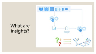
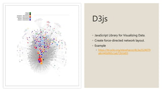
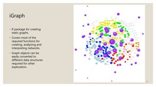
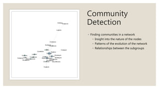
1. Knowledge graphs allow gaining insights through using reasoners, visual analytics, and network science approaches. Reasoners use rules and ontologies while visual analytics uses network visualization libraries. 2. Network science approaches model relationships as nodes and edges. Metrics like degree, betweenness, and centralization quantify properties of individual nodes or the overall network. Community detection identifies subgroups. 3. Comparing networks over time helps understand environmental changes. Mineral co-occurrence networks reveal paragenetic modes through community detection. Evolving networks show how biological utilization of elements changed through Earth's history.

1. Insights from Knowledge Graphs
Anirudh Prabhu,
Keck Deep Time Data Infrastructure Team
and the Deep Carbon Observatory Data Science Team
@Anirudh_14

2. What are
insights?

3. How do we gain insights?
Reasoners
Visual Analytics
Network Science Approach

4. Reasoners

5. ONTOLOGY
5

6. Rules Engine – Apache Jena Example
[hurricane-half-hourly:
(?candidate dd:candidateEvent ?event),
(?event rdf:type dd:Hurricane),
(?candidate dd:candidateVariable ?variable),
(?variable dd:timeInterval ?timeInterval),
equal(?timeInterval, <http://darkdata.tw.rpi.edu/data/time-interval/half-hourly>),
makeSkolem(?assertion, dd:Hurricane, ?timeInterval)
->
(?candidate dd:compatibilityAssertion ?assertion),
(?assertion rdf:type dd:CompatibilityAssertion),
(?assertion dd:compatibilityValue dd:strong_compatibility),
(?assertion dd:assertionConfidence "0.5"^^xsd:double),
(?assertion dd:basisForAssertion <urn:rule/time_interval/hurricane-half-hourly>)
]
‘Half hourly’ time interval is best for Hurricanes and Tropical Storms.
Antecedent :
Containing
information about
Phenomena and
Temporal
Resolution.
Subsequent :
Containing the
compatibility
assertion
information.
6

7. Visual
Analytics

8. Visual Analytics
◦D3js/Visjs
◦VOWL
◦iGraph/VisNetwork

9. What is
encoded vs
What is
seen
Encoded Seen/Inferred/Calculated
Nodes Patterns in the Network Geometry
Edges Sub-Communities formed in the
Network
Layout (Mostly Force Directed) Important Hubs in the Network
Additional Parameters for Nodes
(Optional)
Additional metrics that explain the
complexity of the environment
(assortativity, betweenness,
centrality etc.)
9
• Comparison of how different networks change through time also
help understand the given environment.

10. VOWL

11. D3js
◦ JavaScript Library for Visualizing Data.
◦ Create force-directed network layout.
◦ Example
◦ https://bl.ocks.org/steveharoz/8c3e2524079
a8c440df60c1ab72b5d03

12. iGraph
◦ R package for creating
static graphs.
◦ Covers most of the
required functions for
creating, analyzing and
interpreting networks.
◦ Graph objects can be
easily converted to
different data structures
required for other
exploration.
12
Pb
U
P
Al
As
Cu
Ca
K
Na
C
S
Si
V
Ba
Fe
Mg
Mo
Se

13. visNetwork
◦ R package written using the
Javascript library.
◦ Easier to deal with data
structures in R, than using
JavaScript.
◦ The data objects from the
network can be directly used
for further analysis.

14. Coexisting Animal Families through last 542 million years
Animal Family Networks

15. Ediacaran Assemblage Networks
Extinction Event
at 560 Ma?
Drew Muscente: “Nama and White Sea fauna are different facies,
whereas a mass extinction occurred after the Avalonian.” – science
hypothesis

16. Network
Science
Approach

17. Libraries/Packages
17
Igraph
ggnetwork
Network
SNA
visNetwork
D3js
Threejs
ngraph

18. Data Structure
• Symmetric adjacency matrix
• Rows and column names represent mineral species
• Values represent co-occurrence of 2 minerals
Node List and Properties
Adjacency Matrix

19. Data Structures (contd.)
• Nodes• Links

20. What is
encoded vs
What is
seen
Encoded Seen/Inferred/Calculated
Nodes Patterns in the Network Geometry
Edges Sub-Communities formed in the
Network
Layout (Mostly Force Directed) Important Hubs in the Network
Additional Parameters for Nodes
(Optional)
Additional metrics that explain the
complexity of the environment
(assortativity, betweenness,
centrality etc.)
20
• Comparison of how different networks change through time also
help understand the given environment.

21. Network
Metrics

22. Comparing
Global
Metrics
22

23. Assortativity
(Homophily)
◦ Network equivalent of
Pearson correlation
coefficient
◦ Values between 1 & -1
◦ 1 = similarity favors
connections
◦ 0 = non-assortative
◦ -1 = opposites attract
23
•Muscente AD, Prabhu A, Zhong H, Eleish A, Meyer M,
Fox P, Hazen R, and Knoll A (2017) The network
paleoecology of mass extinctions. PNAS.

24. Community
Detection
◦ Finding communities in a network
◦ Insight into the nature of the nodes
◦ Patterns of the evolution of the network
◦ Relationships between the subgroups

25. Walktrap algorithm

26. Example : Mineral Co-occurence
26
Morrison SM, Liu C, Eleish A, Prabhu A, Li
C, Ralph J, Downs RT, Golden JJ, Fox P,
Hummer DR, Meyer MB, and Hazen RM
(2017) Network analysis of mineralogical
systems. American Mineralogist 102
• Groups correspond to Paragenetic Mode.
• Paragenetic Mode : Formation Conditions.
• How and when the Minerals were formed.

27. Example : Evolving Networks
27
Moore, E. K., Hao, J., Prabhu,
A., Zhong, H., Jelen, B. I.,
Meyer, M., ... & Falkowski, P.
G. (2018). Geological and
Chemical Factors that
Impacted the Biological
Utilization of Cobalt in the
Archean Eon. Journal of
Geophysical Research:
Biogeosciences.

28. Simple Examples
◦ https://jupyter.deepcarbon.net/user/anirudhprabhu/notebooks/Code/R
FM_Network.ipynb
◦ https://deeptime.tw.rpi.edu/jupyter/user/6d32485f-bcb8-473e-99fe-
66ce2f2a4e44/notebooks/U/U_minerals_deposit_types.ipynb

29. Thank You
Questions?

30. Metrics: Local
Degree is the number of links connected to a given node.
35
1 2
2
3
0.56
0 0
0.5
0
10
1
1
Betweenness is a measure of the number of geodesic
paths that pass through a given node.
Distance is the geodesic (shortest) between any
two nodes.

31. Metrics: Global
Density, D, is the no. of links divided by
the no. of possible links
D = 0.66 D = 1D = 0.33
Low density High density
D =
2𝐿
𝑁(𝑁−1)

32. Metrics: Global
Diameter: largest geodesic distance in a network (the
shortest path between the two most separated nodes)
Mean Distance: average “degree of separation” in a
network

33. Metrics: Global
Centralization:
A measure of how central a network’s ”most central” node is relative to how
central all the other nodes are.
• Degree centralization: number of links to each node
• Are there many highly interconnected nodes?
• Betweenness centralization: number of shortest paths through
each node
• Are there a few key “broker” nodes?