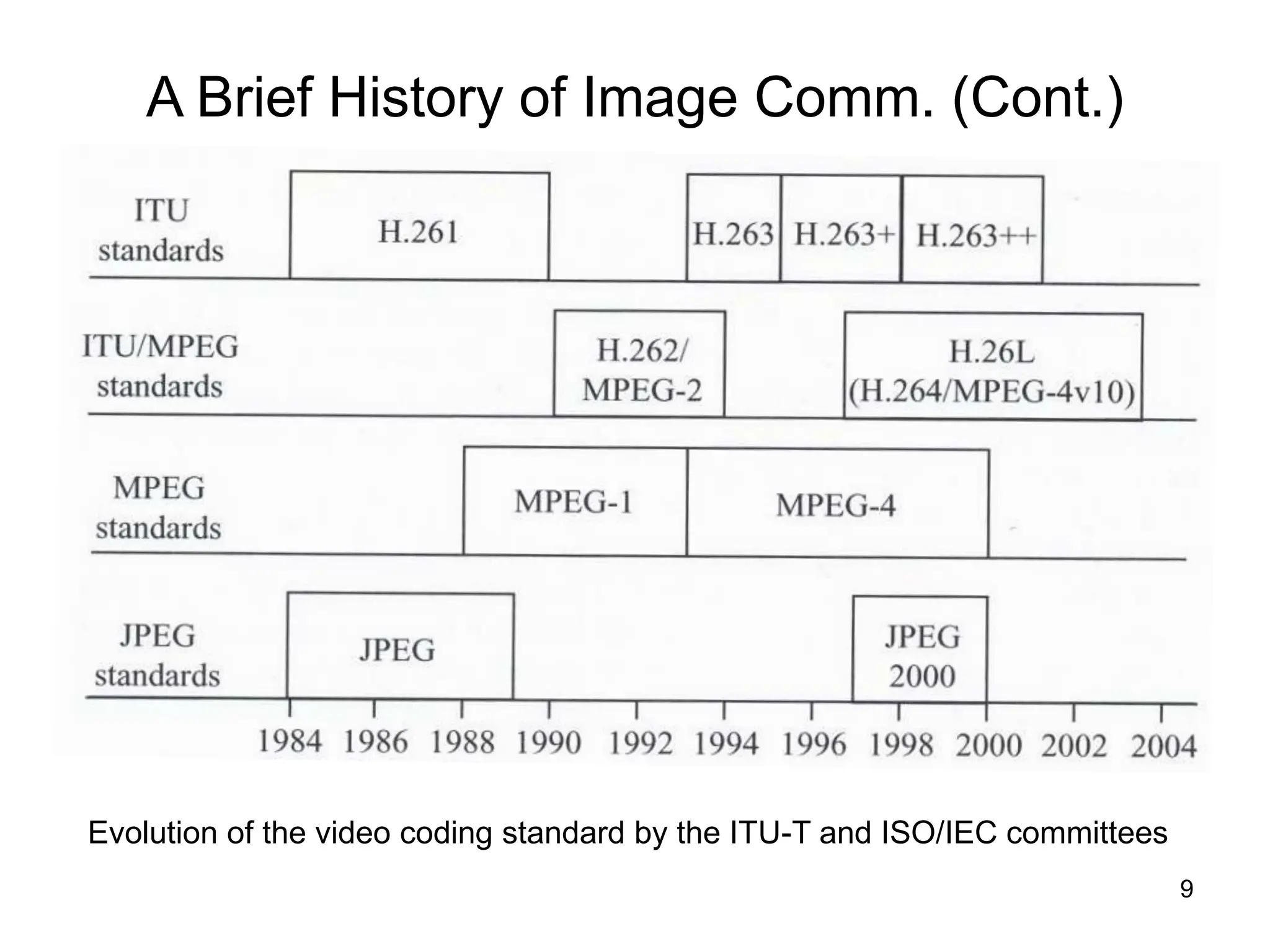
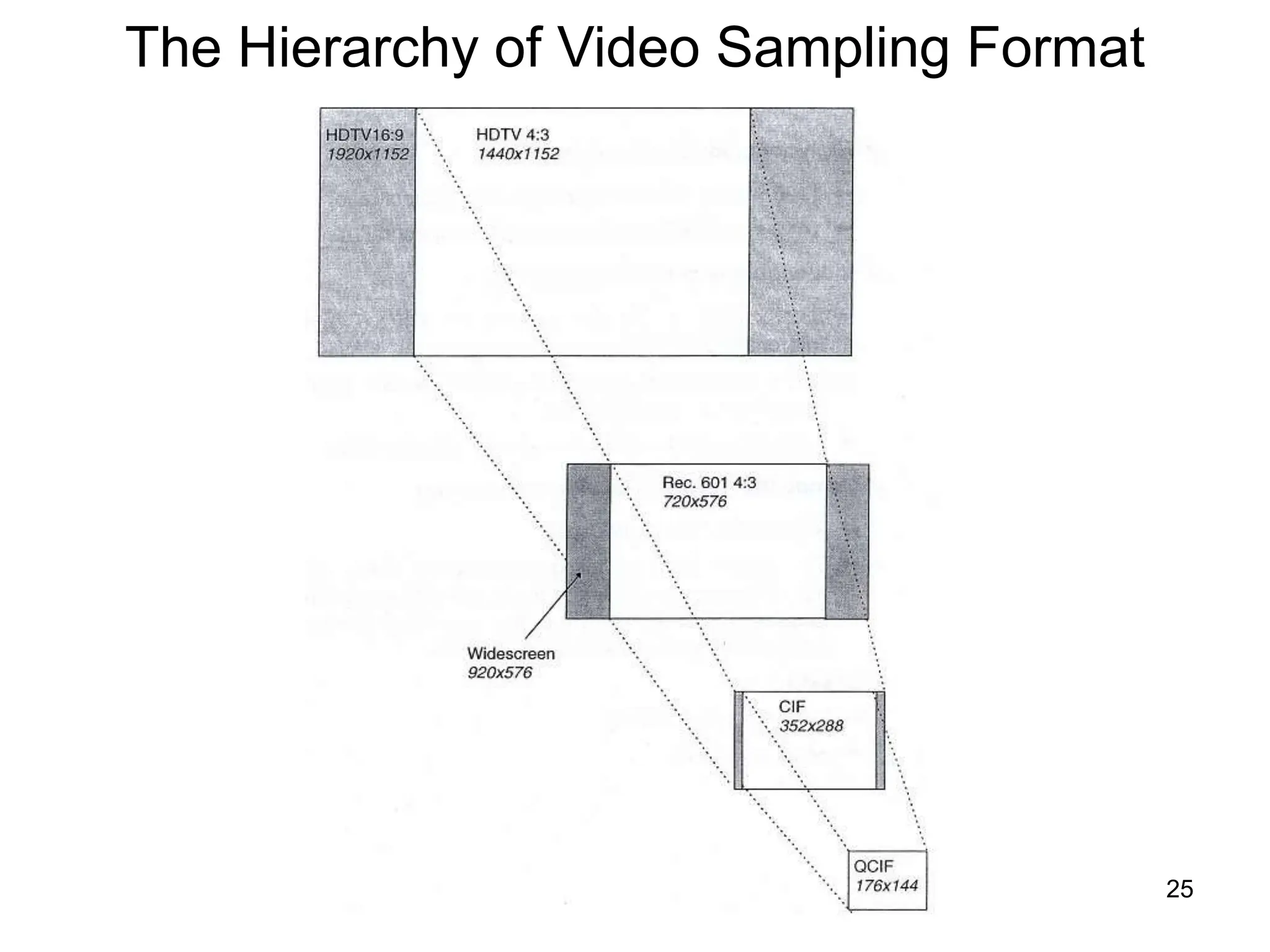
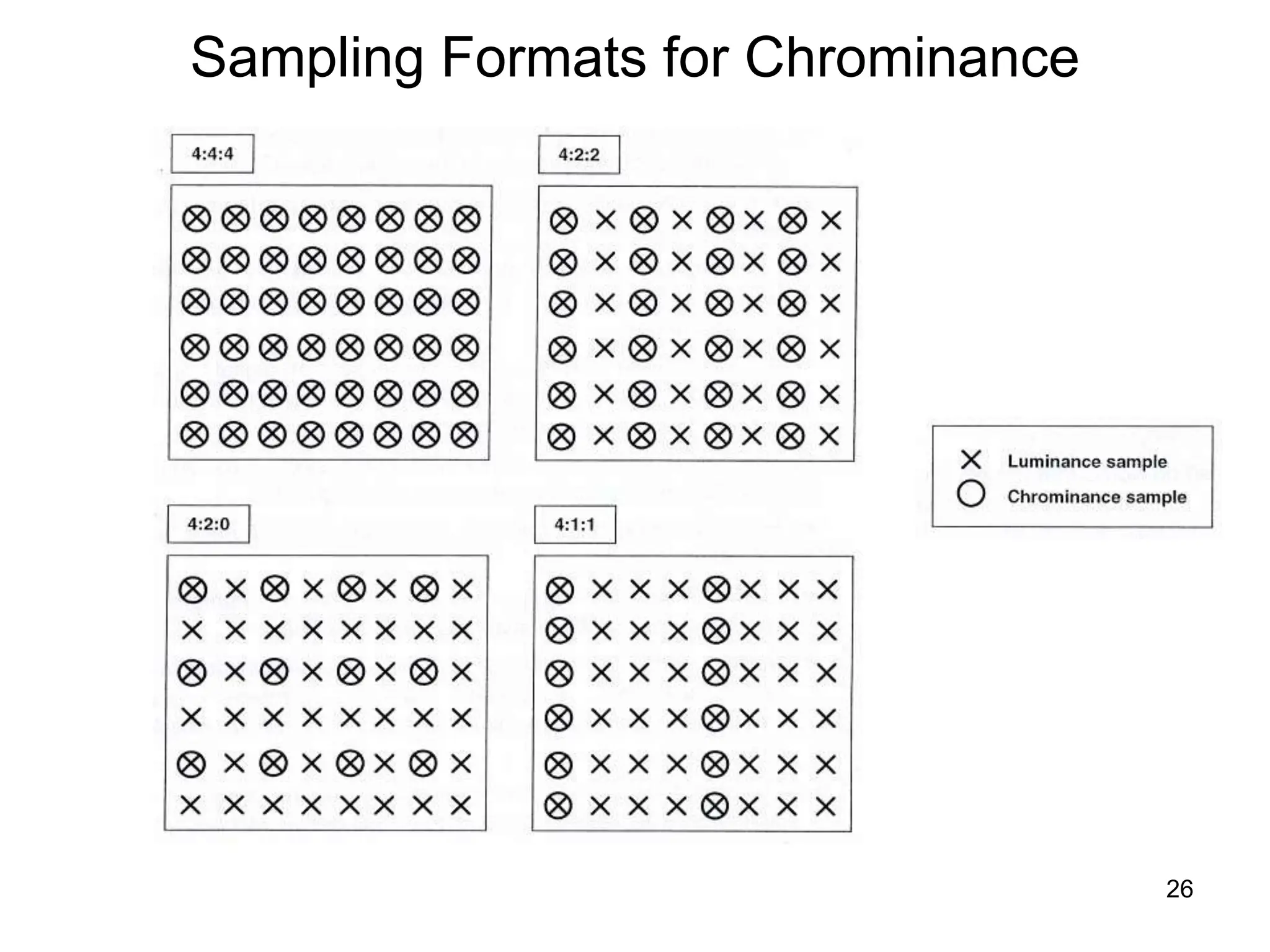
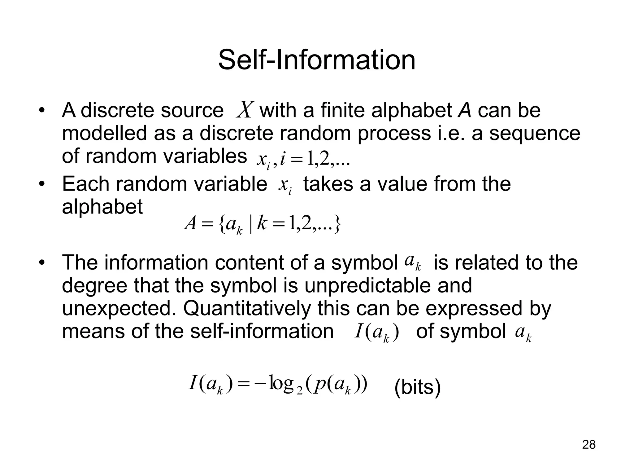
SlideShare a Scribd company logo
1 of 79
1
Image and Video Compression
Wenwu Wang
Centre for Vision Speech and Signal Processing
Department of Electronic Engineering
University of Surrey
Email: w.wang@surrey.ac.uk
2
Introduction
• Course components
• A brief history
• Basic concepts
• Coding performance limits
• Coding of still image
3
Course Components
• Component Coding Algorithms I (By myself)
 Fundamentals of Compression
 Coding of Still image
 JPEG standard
 Vector Quantisation
 Subband and Wavelet Coding
• Component Coding Algorithms II (By Dr Fernando)
 Coding of video sequence,
 H.261, 263, coding algorithms
 MPEG-1, -2, -4 coding algorithms
• Component Error Resilience in Video
Communications (By Prof. Kondoz)
4
Further Reading
• Component Coding Algorithms
• Ghanbari, M. Standard Codecs: Image Compression to Advanced Video Coding, IEE
Telecommunication Series 49, 2003. 0-85296-710-1 A
• Clarke, R. J. Digital Compression of Still Images and Video, Academic Press, 1995. 0-12-175720-X B
• Haskell, B. G., Puri, A. and Netravali, A. N. Digital Video: An Introduction to MPEG-2, Chapman and
Hall, 1997. 0-412-08411-2 B
 Error Resilience
• Sadka, A. H. Compressed Video Communications, J. Wiley and Co, 2001. 0-470843128 A
 More References
5
A Brief History of Image Communication
• 1840 Louis J.M. Daguerre, France,
William Henry Fox Talbot, USA, photographic film
• 1895 First public motion picture presentation
• 1920s First television experiment
British TV pioneer J.L. Baird with Nipkow Disc (around 1926)
6
A Brief History of Image Comm. (Cont)
• 1930s Color movies
• 1930-32 First experimental television broadcasting in US
• 1935 First German television broadcasting in Berlin
• 1936 TV transmission during the Berlin Olympics
British TV pioneer J.L. Baird with Nipkow Disc (around 1926)
7
A Brief History of Image Comm. (Cont.)
• 1939 Regular monochrome TV service in US
• 1952 Regular TV service in Germany
• 1954 NTSC Color television in US
• 1967 PAL color television in Germany
• 1970s Consumer video cassette recorder (VCR)
• 1970s Fax machines
• 1980s Digital TV studios (ITU-R rec. 601)
8
A Brief History of Image Comm. (Cont.)
• 1990s JPEG and MPEG standards
Digital still cameras
Digital TV broadcasting
Digital video/versatile disk (DVD)
Integration of computers and video
World wide web
Internet video streaming
9
A Brief History of Image Comm. (Cont.)
Evolution of the video coding standard by the ITU-T and ISO/IEC committees
10
Fundamentals
11
What?
• The minimisation of the amount of information required
to represent an image/video signal
• The reduction of the overall signal bandwidth
12
Why?
• Applications for which bandwidth is a precious
commodity
• Storage applications:
Archiving, television production, home entertainment,
multimedia
• Transmission applications:
Radio and television broadcasting, internet video
streaming, multimedia for mobile phones
13
How?
• Image and video signals contain superfluous
(redundant) information
• Statistical redundancy associated with signal
predictability/correlation/smoothness:
Original signal can be recovered perfectly, therefore it is
called “lossless” or “information preserving” coding
• Subjective redundancy associated with the error
tolerance of human vision:
Original signal cannot be recovered perfectly, only an
approximate reconstruction is possible, therefore it is
called “lossy” or “error tolerant” coding
14
Performance Assessment
• Efficiency in image and video coding
(an indication of how much information has been reduced for the coded
signal)
 lossless systems: ratios of uncoded-to-coded
information, i.e. compression ratio
 lossy systems: the amount of coded information
expressed as a function of the distortion introduced by
the coding operation, i.e. rate/distortion function
• Distortion in image and video coding
(an indication of how close to the original is the coded signal)
 lossless systems: trivially zero distortion (infinite fidelity)
 lossy systems: distortion can be measured objectively
(computation of error between the original and the coded
representation) or subjectively (tests designed to
measure response of human vision to coding artefacts)
15
Coding Operation in the Image Chain
• Signal processing operations anywhere in the image chain
can be regarded as coding operations. Such operations
may be due to:
 Acquisition environment (such as lighting conditions and light
propagation, special effects in studio, and atmospheric conditions in
outside broadcasts)
 Acquisition systems (such as camera optics, scanning aperture and
field integration in electronic imaging, and chemical process in film)
 Post-production environment (such as special effects)
 Image/video display systems (such as display aperture in electronic
imaging, half-toning in printed media, and chemical process in film)
 Viewing environment (such as propagation of light, and optical paths)
 Human visual system (such as lens, and response of neurons to light
stimuli)
• We are not concerned with the above but need to be aware of their
coding effects.
• We are concerned with the processing of image/video signals after
acquisition/post-production and prior to display
16
Classification of Video Coding Sytems
• Analogue (signals predominantly in analogue form)
 PAL (Phase Alternating Line, transmission of terrestrial television)
 VHS (Video Home System, home video recording)
 MAC (Multiplexed Analogue Component, satellite television transmission)
 Betacam SP (Superior Performance, video recording in the studio)
• Digital (signals predominantly in digital form)
 ITU-R Rec. 601 (BT.601, or CCIR-601) (professional video recording)
 MPEG-1 (home video recording, CD-ROM)
 MPEG-2 (television transmission)
 MPEG-4 (multimedia)
 H.261/3 (video conferencing)
 JPEG (still images)
• We will be mainly concerned with digital signals in this module.
For more about analogue signals, please refer to some
textbooks. Here, we only introduce a few fundamentals about
analogue signals that closely related to digital signals.
17
Coding of Colour Signals
• One of the challenges facing the first of colour
television systems was the inclusion of colour
information without increasing the video bandwidth.
• Colour cameras operate in the space of R,G,B
primaries. Each of these component signals are full-
bandwidth (i.e. 6.75MHz)
• Colour coding systems (i.e. PAL) typically involve the
conversion of component signals to composite by
means of the following processing operations:
 R,G,B to Y,U,V co-ordinate transformation
 Low-pass filtering of U and V components
 DSSC-AM modulation of U and V by two sub-carriers in phase
quadrature
 Sign alternation of modulated V at every other line
18
Coding of Colour Signals (Cont.)
587
.
0
,
114
.
0
,
299
.
0
,
)
1
/(
)
(
615
.
0
)
1
/(
)
(
436
.
0














G
B
R
R
B
B
G
R
W
W
W
where
W
Y
R
V
W
Y
B
U
B
W
G
W
R
W
Y
19
Coding of Colour Signals (Cont.)
• Y – Luma component, representing the brightness of
an image (i.e. the “black and white” or achromatic
portion of the image).
• U – Blue difference chroma (B-Y)
• V – Red difference chroma (R-Y)
• “Luma” and “chroma” are usually used in video
engineering, while “luminance” and “chrominance” are
used in color science.
• In digital domain, YCbCr is used to represent the
coded color, where DSSC-AM modulation is replaced
by subsampling.
20
Consequence of Colour Coding
• Compression ration: 3:1
• Artefacts
 Visible line structure, and interline flicker,
 Combing (distortion of vertical detail moving horizontally due to interlace)
 Spatial aliasing (i.e. diagonal straight lines cause spatial “beat” frequencies
and jagged/staircase edges)
 Temporal aliasing (fast motion suffers from “judder”)
 Picture “softness” (aperture effects)
• Artefact frequency: low
• Artefact severity: high
• Remedies
 At the transmitter end, intelligent PAL encoding allowing better segregation
of colour and monochrome components with less crosstalk between them
 At the receiver end, intelligent PAL decoding possibly involving motion
adaptive filtering (may attenuate some frequency components)
21
Digital Video Formats – A Case Study of
Digital Television
• This format is standardised and is described in the document
“Recommendation ITU-R BT.601”.
• Source signals: Y,U,V (one luminance and two colour-difference
components, gamma pre-corrected and filtered)
• Sampling structure (625 line/50Hz analogue system)
 Orthogonal, line, field and frame repetitive
 U,V samples co-sited with odd Y samples in each line
 864 total (720 active) luminance samples per line
 432 total (360 active) chrominance samples per line
 625 total (576 active) lines
• Sampling frequency (Y:135MHz, U,V:6.75MHz)
• Quantisation
 Uniformly quantised PCM
 8 (optionally 10) bits per sample
 Scale 0-255
 Luminance black level defined as level 16
 Luminance peak white level defined as level 235
 Luminance total number of active levels 220
 Chrominance total number of active levels 225 with zero corresponding to 128
22
Digital Video Formats – A Case Study of
Digital Television (Cont.)
• Total active bit-rate
 720 samples/line X 576 lines/frame X 25 frames/sec X 8
bits/sample/component X (1+0.5+0.5) components = 166 Mbits/sec
• Total raw bit-rate (Y:135MHz, U,V:6.75MHz)
 864 samples/line X 625 lines/frame X 25 frames/sec X 8
bits/sample/component X (1+0.5+0.5) components = 216 Mbits/sec
 For television transmission purposes this amount of
information may require (depending on the modulation
scheme) a bandwidth of 40 MHz upwards
 Today this corresponds to occupancy requirements of 6-7
analogue terrestrial television channels !! Therefore, to
make digital television transmission a practical proposition
compression in the digital domain is imperative.
23
Digital Video Formats – A Case Study of
Digital Television (Cont.)
• Note 1
 Unused samples and levels are actually used to convey auxiliary and
control information i.e. vertical and horizontal synchronisation
(blanking), colour reference (burst) etc. There are applications which
require this information in digital form
• Note 2
 The 601 standard is a specification of the output format only and is
not concerned with the practical implementation of the A/D
conversion. This is left to the system designer to implement but
should typically involve anti-aliasing pre-filtering and attention to the
effects of the non-ideal sampling aperture and pixel aspect ratio.
24
Digital Video Formats – Other Formats
• High-definition television (HDTV)
 1920 X 1152 X 50 Hz interlaced (16:9 aspect ratio)
 1440 X 1152 X 50 Hz interlaced (4:3 aspect ratio)
• Video-conferencing/Video-telephony
 352 X 288 X 30 Hz Progressive CIF (Common Interchange Format)
 352 X 288 (240) X 25 (30) Hz progressive SIF (Source Input Format-PAL
(NTSC))
 176 X 144 X 30 Hz Progressive QCIF (Quarter CIF)
• Composite (PAL) digital video (recording)
 922 X 576 X 50 Hz interlaced
 This results from sampling a composite (PAL) signal with a frequency which
is 4 times the colour subcarrier frequency and is used for the recording of
digital composite signals for studio applications
• Desktop
 800 X 600 Super VGA (Vector Graphic Array)
 640 X 480 VGA
25
The Hierarchy of Video Sampling Format
26
Sampling Formats for Chrominance
27
Coding Performance Limits and Assessment
28
Self-Information
• A discrete source with a finite alphabet A can be
modelled as a discrete random process i.e. a sequence
of random variables
• Each random variable takes a value from the
alphabet
• The information content of a symbol is related to the
degree that the symbol is unpredictable and
unexpected. Quantitatively this can be expressed by
means of the self-information of symbol
(bits)
X
,...}
2
,
1
|
{ 
 k
a
A k
i
x
,...
2
,
1
, 
i
xi
k
a
k
a
)
( k
a
I
))
(
(
log
)
( 2 k
k a
p
a
I 

29
Source Models
• Two useful source models are used for the studying the coding
performance limit:
 The Discrete Memoryless Source (DMS)
Successive symbols are statistically independent i.e. in a symbol
sequence the current symbol does not depend on any previous
one
 The Markov K-th order Source (MKS)
Successive symbols are statistically dependent i.e. in a symbol
sequence the current symbol depends on the K previous ones
The entropy of a DMS source X is defined as the average self-
information:
The entropy is maximised for a uniform symbol distribution.

 


k
k
k
k
k
k a
a
p
a
I
a
p
X
H )
(
log
)
(
)
(
)
(
)
( 2
30
Markov-K Source
• The MKS model is a more realistic model for images and video
 Images (of natural scenes) are correlated in the spatial domain i.e. plain
areas (with little or no spatial detail)
 Video is correlated in the spatial domain as above and also in the temporal
domain i.e. static areas (with little or no motion)
• A MKS can be specified by the following conditional probabilities:
• The entropy of a MKS source is defined as
k
i
X
X
a
X
p k
i
i
k
i ,
)
,...,
|
( 1 
 

k
i
X
X
X
H
X
X
a
X
p
X
H
k
S
k
i
i
k
i
i
k
i ,
)
,...,
|
(
)
,...,
|
(
)
( 1
1 

  



where is the conditional entropy i.e.
)
,...,
|
( 1 k
i
i X
X
X
H 

 


 

i
k
i
i
k
i
k
i
i
k
i X
X
a
X
p
X
X
a
X
p ))
,...,
|
(
(
log
)
,...,
|
( 1
2
1
and denotes all possible realisations
k
S }
,...,
{ 1 k
i
i X
X 

31
Coding Theorem
32
Coding Theorem (cont.)
A typical rate distortion curve
33
Practical Considerations
• Information rate for coded still images:
 Bits per pixel (bpp) i.e. the ratio of coded information in bits to the total
number of pixels
 Compression ratio (dimensionless) i.e. the ratio of uncoded-to-coded
information
• Information rate for coded moving sequences:
 Bits per second (b/s) and its multiples (kb/s, Mb/s) i.e. the rate of flow of the
coded information
• Distortion of coded-and-decoded image/video:
 Objectively using the Peak Signal-to-Noise Ratio (PSNR)
 Subjectively using quality and impairment scales designed to measure the
response of human vision. For television, subjective assessment
procedures are standardised and are described in Rec. ITU-R BT. 500
variance
error
coding
levels)
active
of
(#
log
10
2
10

PSNR
34
Subjective Picture Assessment for Television
35
Human Visual System
Plot of contrast sensitivity (just perceptual modulation) function
36
Human Visual System (Cont.)
37
Coding of Still Images
38
Classification of Compression Techniques
• Spatial (data) Domain
Elements are used “raw” in suitable combinations. The
frequency of occurrence of such combinations is used to
influence the design of the coder so that shorter
codewords are used for more frequent combinations and
vice versa (entropy coding).
• Transform Domain
Elements are mapped onto a different domain (i.e. the
frequency domain). The resulting coefficients are
quantised and entropy-coded.
• Hybrid
Combinations of the above.
39
Lossless Coding in the Spatial Domain
• Memoryless Coding
40
Lossless Coding in the Spatial Domain (Cont.)
• Conditional Coding
Construct “current” symbol histograms according to “previous”
symbols and use separate codebooks accordingly
41
Lossless Coding in the Spatial Domain (Cont.)
• Block (joint) Coding
 Define blocks of more than one symbols and record their occurrences using a
multi-dimensional histogram
 Code book grows exponentially with block size
 Useful when symbols in a block are correlated
An example using a block size
of 2 i.e. two consecutive
symbols.
42
Lossless Coding in the Spatial Domain (Cont.)
• Predictive Coding (previous symbol)
 “Previous” symbol used as a prediction of “current” symbol
 Prediction error coded in a memoryless fashion
 Prediction error alphabet and codebook have twice the size
i.e. symbol alphabet {1, 2, 3, 4} prediction alphabet {-3, -2, -1, 0, 1, 2, 3}
 A good predictor will minimise the error (most occurrence will be zero)
43
Lossless Coding in the Spatial Domain (Cont.)
• Predictive Coding (generalised)
 Prediction is based on combination of
previous symbols
 Prediction template needs to be “causal” i.e.
template should contain only “previous”
elements w.r.t the direction of scanning
(shown with arrows). This is important for
coding applications as the decoder will need
to have decoded the template elements first to
perform the prediction of the current element.
44
Lossless Coding in the Spatial Domain (Cont.)
• Run-length Coding
 Useful when consecutive symbols in a string are identical
 A symbol is followed by the number of its repetitions
A typical example
A general example
45
Lossless Coding in the Spatial Domain (Cont.)
• Zero Run-length Coding
 Useful for strings containing long runs of consecutive zeros and are
sparsely populated by non-zero symbols i.e. quantised frame
differences
 A non-zero symbol is followed by the number of consecutive zeros
A typical example
A general example
46
Entropy Coding (Variable Length Coding)
• Assignment of codewords to individual symbols or collections of symbols
according to likelihood
• More probable symbols or collections of symbols are assigned shorter
codewords and vice-versa, so called variable length coding (VLC)
• There are two types of VLC, which are employed in the standard video
codecs: Huffman coding and arithmetic coding.
• Huffman coding is a simple VLC code, and it is suboptimal since its
compression can never reach as low as the entropy due to the constraint
that the assigned symbols must have an integral number of bits. It is
employed in all standard codes.
• Arithmetic coding is an optimal coding method which can approach the
entropy since the symbols are coded collectively using a code string,
which represent a fractional value on the number line between 0 and 1. It
is employed in JPEG, JPEG2000, H.263 and MPEG-4, where extra
compression is demanded.
47
Huffman Coding
48
Huffman Coding (Cont.)
An example of Huffman
code for seven symbols
Entropy:
Average bit per symbol:
49
Arithmetic Coding
• Using a scale in which the coding intervals of real
numbers between 0 and 1 are represented. This is in
fact the cumulative probability density function of all the
symbols which add up to 1.
• The interval is partitioned according to symbol likelihood.
• The interval is iteratively reduced by retaining, at each
iteration, the sub-interval corresponding to the currently
encoded input symbol
50
Arithmetic Coding (cont.)
• An example: suppose the alphabet is {a,e,i,o,u,!} and the fixed model is used with the
probabilities shown in the following table.
• Each individual symbol needs to be assigned a portion of the [1,0) range that
corresponds to its probability of appearance in the cumulative density function. For
example, the alphabet u with probability 0.1 can, defined in the range of [0.8, 0.9),
can take any value from 0.8 to 0.89999…
• Suppose a message eaii! needs to be coded. The first symbol to be encoded is e.
Hence, the final coded message e has to be a number in the range of [0.2, 0.5). The
second symbol is a which is in the range of [0.0, 0.2), but in the subrange of [0.2,
0.5), as it is not the first number to be encoded. Consequently, after the second
symbol, the number is restricted to the range of [0.2+0.0*(0.5-0.2) 0.2+0.2*(0.5-0.2))
= [0.2 0.26)
51
Arithmetic Coding (cont.)
• The next symbol to be encoded is I, in the range of [0.5, 0.6), that corresponds to the
new subrange [0.2, 0.26). Hence, after this symbol, the coded number is restricted to
the range of [0.2+0.5*(0.26-0.2), 0.2+0.6*(0.26-0.2)) = [0.23, 0.236). Applying the
same rule to the successive symbols. We can obtain the following table:
• The final range [0.23354, 0.2336) represents the message eaii!. This means if we
transmit any number in the range of [0.23354, 0.2336), that number represents the
whole message of eaii!.
52
Arithmetic Coding (cont.)
Representation of arithmetic coding process with the interval
scaled up at each stage for the message eaii!
53
Arithmetic Coding (cont.)
• Decoding process
 For the previous example, suppose a number 0.23355 in the range of [0.23354,
0.2336) is transmitted. The decoder, using the same probability intervals as the
encoder, performs a similar procedure.
 Only the interval [0.2, 0.5) of e envelops the transmitted code of 0.23355. So the first
symbol can only be e. The new code for the second symbol is (0.23355-0.2)/(0.5-
0.2)=0.11185, which is enveloped by interval [0.0, 0.2) of symbol a. The new code for
the third symbol is (0.11185-0.0)/(0.2-0.0) = 0.55925, which is enveloped by the range
of [0.5, 0.6) of symbol i. Followed by (0.55925-0.5)/(0.6-0.5) = 0.5925 in the range of
[0.5, 0.6) of symbol i. Further followed (0.5925-0.5)/(0.6-0.5) = 0.925, which is in the
range of [0.9, 1) of symbol !. Therefore, the decoded message is eaii!. The decoding
process is shown in the following table:
54
Lossless Coding in Transform Domain
• Transforms commonly refer to expansions of
signals to series of coefficients using sets of
appropriate (i.e. orthonormal) basis functions so
that the following are achieved.
 Decorrelation of input data
 Optimal distribution of energy (variance) into the smallest number
of coefficients
• The optimal transform according to the above is
the Karhunen-Loeve (KL) transform. This is not
used in practice:
 Its basis functions are the eigenvectors of the covariance matrix of the
input signal, and hence data-dependent, and therefore need to be
computed and transmitted for each data set.
 There are no fast implementations for the KL transform
55
Lossless Coding in Transform Domain (cont.)
• In practice, sub-optimal transforms are used whose basis
functions are data-independent and their performance is
close to the KL transform, such as
56
Lossless Coding in Transform Domain (cont.)
• The DCT is the most widely used transform in image/video coding and is a
fundamental component of many standardised algorithms.
 KLT and DCT basis functions closely resemble each other for images modelled as first-
order Markov processes.
 A n-point DCT is equivalent to a 2n-point DFT obtained by reflection. This avoids
spurious harmonics due to discontinuities at the boundaries of the repetition period.
• The following example visualises the decorrelation and energy compaction
properties of transforms:
57
Lossless Coding in Transform Domain (cont.)
58
Comparison of Various Transforms
59
Comparison of Various Transforms (cont.)
(1) Energy concentration measured typical natural images of block size 1-by-32.
(2) KLT is optimum and DCT performs slightly worse than KLT
60
Block Transform Coding
61
Block Transform Coding (cont.)
62
Block Transform Coding (cont.)
63
Lossy Coding
• For natural images the compression performacne of lossless
coding schemes is fairly modest
 Compression ratios of 3:1 or 4:1 can be achieved using the best of the
above mentioned schemes.
 This is comparable to the performance achieved by the general purpose
data compression algorithms i.e. Ziv-Lempel, which are not designed
specifically to exploit image structure.
• To improve performance some coding distortion will have to be
tolerated. The main aims of lossy coding are:
 To optimise rate/distortion performance i.e. achieve the best image quality
for a given target bit-rate
 To minimise the perceptual impact of distortion i.e. produce coding errors
that are likely to be imperceptible to the human viewer
64
Lossy Coding (cont.)
• The main tool for lossy coding is quantisation. This is
applicable to most domains:
 Spatial (data) domain: applicable to raw pixels, pixel differences (predictive
coding), conditional pixel occurrences (conditional coding), ensembles of
pixels (joint coding). This is a special case of so-called vector quantisation
which will be studied separately.
 Transform domain: applicable to transform coefficients and ensembles of
coefficients (vector quantisation).
• Another important tool is sampling
 This is usually applicable to the data domain.
65
Quantisation (scalar)
66
Lossy Predictive Coding
Open-loop encoder
(prediction based on
past inputs)
Closed-loop encoder
(prediction based on
past outputs)
Decoder (prediction
always based on past
outputs)
67
Lossy Transform Coding
Coder
Decoder
68
Sampling: One-dimensional sampling
69
Sampling: One-dimensional sampling (cont.)
70
Sampling: Two-dimensional sampling
71
Sampling: Two-dimensional sampling (cont.)
72
Sampling: Two-dimensional sampling (cont.)
73
Non-ideal Sampling
74
Interpolation
75
Non-ideal Interpolation (sample-and-hold)
76
Non-ideal Interpolation (bi-linear)
77
Example of Non-ideal Interpolation
78
Summary
 A brief history of image communication and
coding standard
 Coding performance theorem
 Some fundamental concepts of compression
 Coding methods for still images
(This is the most important part of this lecturing
session)
79
Acknowledgement
 Thanks to T. Vlachos, B. Girod for providing their
lecture notes that have been partly used in this
presentation.
 Thanks also to M. Ghanbari, and part of the
material used here is from his textbook.

More Related Content

Similar to Image and Video Compression, A brief history - Wang.ppt

simple video compression
simple video compression simple video compression
simple video compression LaLit DuBey
 
Chapter 3 - Fundamental Concepts in Video and Digital Audio.ppt
Chapter 3 - Fundamental Concepts in Video and Digital Audio.pptChapter 3 - Fundamental Concepts in Video and Digital Audio.ppt
Chapter 3 - Fundamental Concepts in Video and Digital Audio.pptBinyamBekele3
 
Tutorial High Efficiency Video Coding Coding - Tools and Specification.pdf
Tutorial High Efficiency Video Coding Coding - Tools and Specification.pdfTutorial High Efficiency Video Coding Coding - Tools and Specification.pdf
Tutorial High Efficiency Video Coding Coding - Tools and Specification.pdfssuserc5a4dd
 
8k RESOLUTION CAMERA SYSTEM
8k RESOLUTION CAMERA SYSTEM8k RESOLUTION CAMERA SYSTEM
8k RESOLUTION CAMERA SYSTEMArun Raj
 
8K RESOLUTION CAMERA SYSTEM
8K RESOLUTION CAMERA SYSTEM8K RESOLUTION CAMERA SYSTEM
8K RESOLUTION CAMERA SYSTEMArun Raj
 
An Introduction to HDTV Principles-Part 1
An Introduction to HDTV Principles-Part 1    An Introduction to HDTV Principles-Part 1
An Introduction to HDTV Principles-Part 1 Dr. Mohieddin Moradi
 
Direct satellite broadcast receiver using mpeg 2
Direct satellite broadcast receiver using mpeg 2Direct satellite broadcast receiver using mpeg 2
Direct satellite broadcast receiver using mpeg 2arpit shukla
 
Presentation12
Presentation12Presentation12
Presentation12fadocs
 
Next generation image compression standards: JPEG XR and AIC
Next generation image compression standards: JPEG XR and AICNext generation image compression standards: JPEG XR and AIC
Next generation image compression standards: JPEG XR and AICTouradj Ebrahimi
 
Chapter 3- Media Representation and Formats.ppt
Chapter 3- Media Representation and Formats.pptChapter 3- Media Representation and Formats.ppt
Chapter 3- Media Representation and Formats.pptVasanthiMuniasamy2
 
Unit ii mm_chap5_fundamentals concepts in video
Unit ii mm_chap5_fundamentals concepts in videoUnit ii mm_chap5_fundamentals concepts in video
Unit ii mm_chap5_fundamentals concepts in videoEellekwameowusu
 

Similar to Image and Video Compression, A brief history - Wang.ppt (20)

MaxEye DVB Test and Measurement Solutions Overview
MaxEye DVB Test and Measurement Solutions OverviewMaxEye DVB Test and Measurement Solutions Overview
MaxEye DVB Test and Measurement Solutions Overview
 
Image aquation
Image aquationImage aquation
Image aquation
 
simple video compression
simple video compression simple video compression
simple video compression
 
Chapter 3 - Fundamental Concepts in Video and Digital Audio.ppt
Chapter 3 - Fundamental Concepts in Video and Digital Audio.pptChapter 3 - Fundamental Concepts in Video and Digital Audio.ppt
Chapter 3 - Fundamental Concepts in Video and Digital Audio.ppt
 
Tutorial High Efficiency Video Coding Coding - Tools and Specification.pdf
Tutorial High Efficiency Video Coding Coding - Tools and Specification.pdfTutorial High Efficiency Video Coding Coding - Tools and Specification.pdf
Tutorial High Efficiency Video Coding Coding - Tools and Specification.pdf
 
intro_dgital_TV
intro_dgital_TVintro_dgital_TV
intro_dgital_TV
 
intro_dgital_TV
intro_dgital_TVintro_dgital_TV
intro_dgital_TV
 
intro_dgital_TV
intro_dgital_TVintro_dgital_TV
intro_dgital_TV
 
chapter5.pptx
chapter5.pptxchapter5.pptx
chapter5.pptx
 
8k RESOLUTION CAMERA SYSTEM
8k RESOLUTION CAMERA SYSTEM8k RESOLUTION CAMERA SYSTEM
8k RESOLUTION CAMERA SYSTEM
 
8K RESOLUTION CAMERA SYSTEM
8K RESOLUTION CAMERA SYSTEM8K RESOLUTION CAMERA SYSTEM
8K RESOLUTION CAMERA SYSTEM
 
An Introduction to HDTV Principles-Part 1
An Introduction to HDTV Principles-Part 1    An Introduction to HDTV Principles-Part 1
An Introduction to HDTV Principles-Part 1
 
Barcelona keynote web
Barcelona keynote webBarcelona keynote web
Barcelona keynote web
 
Direct satellite broadcast receiver using mpeg 2
Direct satellite broadcast receiver using mpeg 2Direct satellite broadcast receiver using mpeg 2
Direct satellite broadcast receiver using mpeg 2
 
Presentation12
Presentation12Presentation12
Presentation12
 
Next generation image compression standards: JPEG XR and AIC
Next generation image compression standards: JPEG XR and AICNext generation image compression standards: JPEG XR and AIC
Next generation image compression standards: JPEG XR and AIC
 
85 videocompress
85 videocompress85 videocompress
85 videocompress
 
Chapter 3- Media Representation and Formats.ppt
Chapter 3- Media Representation and Formats.pptChapter 3- Media Representation and Formats.ppt
Chapter 3- Media Representation and Formats.ppt
 
Beginning of dtv
Beginning of dtvBeginning of dtv
Beginning of dtv
 
Unit ii mm_chap5_fundamentals concepts in video
Unit ii mm_chap5_fundamentals concepts in videoUnit ii mm_chap5_fundamentals concepts in video
Unit ii mm_chap5_fundamentals concepts in video
 

Recently uploaded

Dashanga agada a formulation of Agada tantra dealt in 3 Rd year bams agada tanta
Dashanga agada a formulation of Agada tantra dealt in 3 Rd year bams agada tantaDashanga agada a formulation of Agada tantra dealt in 3 Rd year bams agada tanta
Dashanga agada a formulation of Agada tantra dealt in 3 Rd year bams agada tantaPraksha3
 
LIGHT-PHENOMENA-BY-CABUALDIONALDOPANOGANCADIENTE-CONDEZA (1).pptx
LIGHT-PHENOMENA-BY-CABUALDIONALDOPANOGANCADIENTE-CONDEZA (1).pptxLIGHT-PHENOMENA-BY-CABUALDIONALDOPANOGANCADIENTE-CONDEZA (1).pptx
LIGHT-PHENOMENA-BY-CABUALDIONALDOPANOGANCADIENTE-CONDEZA (1).pptxmalonesandreagweneth
 
Microphone- characteristics,carbon microphone, dynamic microphone.pptx
Microphone- characteristics,carbon microphone, dynamic microphone.pptxMicrophone- characteristics,carbon microphone, dynamic microphone.pptx
Microphone- characteristics,carbon microphone, dynamic microphone.pptxpriyankatabhane
 
Twin's paradox experiment is a meassurement of the extra dimensions.pptx
Twin's paradox experiment is a meassurement of the extra dimensions.pptxTwin's paradox experiment is a meassurement of the extra dimensions.pptx
Twin's paradox experiment is a meassurement of the extra dimensions.pptxEran Akiva Sinbar
 
Forest laws, Indian forest laws, why they are important
Forest laws, Indian forest laws, why they are importantForest laws, Indian forest laws, why they are important
Forest laws, Indian forest laws, why they are importantadityabhardwaj282
 
Grafana in space: Monitoring Japan's SLIM moon lander in real time
Grafana in space: Monitoring Japan's SLIM moon lander  in real timeGrafana in space: Monitoring Japan's SLIM moon lander  in real time
Grafana in space: Monitoring Japan's SLIM moon lander in real timeSatoshi NAKAHIRA
 
Scheme-of-Work-Science-Stage-4 cambridge science.docx
Scheme-of-Work-Science-Stage-4 cambridge science.docxScheme-of-Work-Science-Stage-4 cambridge science.docx
Scheme-of-Work-Science-Stage-4 cambridge science.docxyaramohamed343013
 
Call Girls In Nihal Vihar Delhi ❤️8860477959 Looking Escorts In 24/7 Delhi NCR
Call Girls In Nihal Vihar Delhi ❤️8860477959 Looking Escorts In 24/7 Delhi NCRCall Girls In Nihal Vihar Delhi ❤️8860477959 Looking Escorts In 24/7 Delhi NCR
Call Girls In Nihal Vihar Delhi ❤️8860477959 Looking Escorts In 24/7 Delhi NCRlizamodels9
 
Neurodevelopmental disorders according to the dsm 5 tr
Neurodevelopmental disorders according to the dsm 5 trNeurodevelopmental disorders according to the dsm 5 tr
Neurodevelopmental disorders according to the dsm 5 trssuser06f238
 
Call Girls in Munirka Delhi 💯Call Us 🔝8264348440🔝
Call Girls in Munirka Delhi 💯Call Us 🔝8264348440🔝Call Girls in Munirka Delhi 💯Call Us 🔝8264348440🔝
Call Girls in Munirka Delhi 💯Call Us 🔝8264348440🔝soniya singh
 
Call Girls in Hauz Khas Delhi 💯Call Us 🔝9953322196🔝 💯Escort.
Call Girls in Hauz Khas Delhi 💯Call Us 🔝9953322196🔝 💯Escort.Call Girls in Hauz Khas Delhi 💯Call Us 🔝9953322196🔝 💯Escort.
Call Girls in Hauz Khas Delhi 💯Call Us 🔝9953322196🔝 💯Escort.aasikanpl
 
Module 4: Mendelian Genetics and Punnett Square
Module 4:  Mendelian Genetics and Punnett SquareModule 4:  Mendelian Genetics and Punnett Square
Module 4: Mendelian Genetics and Punnett SquareIsiahStephanRadaza
 
Evidences of Evolution General Biology 2
Evidences of Evolution General Biology 2Evidences of Evolution General Biology 2
Evidences of Evolution General Biology 2John Carlo Rollon
 
Recombinant DNA technology( Transgenic plant and animal)
Recombinant DNA technology( Transgenic plant and animal)Recombinant DNA technology( Transgenic plant and animal)
Recombinant DNA technology( Transgenic plant and animal)DHURKADEVIBASKAR
 
TOPIC 8 Temperature and Heat.pdf physics
TOPIC 8 Temperature and Heat.pdf physicsTOPIC 8 Temperature and Heat.pdf physics
TOPIC 8 Temperature and Heat.pdf physicsssuserddc89b
 
Is RISC-V ready for HPC workload? Maybe?
Is RISC-V ready for HPC workload? Maybe?Is RISC-V ready for HPC workload? Maybe?
Is RISC-V ready for HPC workload? Maybe?Patrick Diehl
 
Analytical Profile of Coleus Forskohlii | Forskolin .pdf
Analytical Profile of Coleus Forskohlii | Forskolin .pdfAnalytical Profile of Coleus Forskohlii | Forskolin .pdf
Analytical Profile of Coleus Forskohlii | Forskolin .pdfSwapnil Therkar
 
RESPIRATORY ADAPTATIONS TO HYPOXIA IN HUMNAS.pptx
RESPIRATORY ADAPTATIONS TO HYPOXIA IN HUMNAS.pptxRESPIRATORY ADAPTATIONS TO HYPOXIA IN HUMNAS.pptx
RESPIRATORY ADAPTATIONS TO HYPOXIA IN HUMNAS.pptxFarihaAbdulRasheed
 
Spermiogenesis or Spermateleosis or metamorphosis of spermatid
Spermiogenesis or Spermateleosis or metamorphosis of spermatidSpermiogenesis or Spermateleosis or metamorphosis of spermatid
Spermiogenesis or Spermateleosis or metamorphosis of spermatidSarthak Sekhar Mondal
 

Recently uploaded (20)

Dashanga agada a formulation of Agada tantra dealt in 3 Rd year bams agada tanta
Dashanga agada a formulation of Agada tantra dealt in 3 Rd year bams agada tantaDashanga agada a formulation of Agada tantra dealt in 3 Rd year bams agada tanta
Dashanga agada a formulation of Agada tantra dealt in 3 Rd year bams agada tanta
 
LIGHT-PHENOMENA-BY-CABUALDIONALDOPANOGANCADIENTE-CONDEZA (1).pptx
LIGHT-PHENOMENA-BY-CABUALDIONALDOPANOGANCADIENTE-CONDEZA (1).pptxLIGHT-PHENOMENA-BY-CABUALDIONALDOPANOGANCADIENTE-CONDEZA (1).pptx
LIGHT-PHENOMENA-BY-CABUALDIONALDOPANOGANCADIENTE-CONDEZA (1).pptx
 
Microphone- characteristics,carbon microphone, dynamic microphone.pptx
Microphone- characteristics,carbon microphone, dynamic microphone.pptxMicrophone- characteristics,carbon microphone, dynamic microphone.pptx
Microphone- characteristics,carbon microphone, dynamic microphone.pptx
 
Twin's paradox experiment is a meassurement of the extra dimensions.pptx
Twin's paradox experiment is a meassurement of the extra dimensions.pptxTwin's paradox experiment is a meassurement of the extra dimensions.pptx
Twin's paradox experiment is a meassurement of the extra dimensions.pptx
 
Forest laws, Indian forest laws, why they are important
Forest laws, Indian forest laws, why they are importantForest laws, Indian forest laws, why they are important
Forest laws, Indian forest laws, why they are important
 
Grafana in space: Monitoring Japan's SLIM moon lander in real time
Grafana in space: Monitoring Japan's SLIM moon lander  in real timeGrafana in space: Monitoring Japan's SLIM moon lander  in real time
Grafana in space: Monitoring Japan's SLIM moon lander in real time
 
Volatile Oils Pharmacognosy And Phytochemistry -I
Volatile Oils Pharmacognosy And Phytochemistry -IVolatile Oils Pharmacognosy And Phytochemistry -I
Volatile Oils Pharmacognosy And Phytochemistry -I
 
Scheme-of-Work-Science-Stage-4 cambridge science.docx
Scheme-of-Work-Science-Stage-4 cambridge science.docxScheme-of-Work-Science-Stage-4 cambridge science.docx
Scheme-of-Work-Science-Stage-4 cambridge science.docx
 
Call Girls In Nihal Vihar Delhi ❤️8860477959 Looking Escorts In 24/7 Delhi NCR
Call Girls In Nihal Vihar Delhi ❤️8860477959 Looking Escorts In 24/7 Delhi NCRCall Girls In Nihal Vihar Delhi ❤️8860477959 Looking Escorts In 24/7 Delhi NCR
Call Girls In Nihal Vihar Delhi ❤️8860477959 Looking Escorts In 24/7 Delhi NCR
 
Neurodevelopmental disorders according to the dsm 5 tr
Neurodevelopmental disorders according to the dsm 5 trNeurodevelopmental disorders according to the dsm 5 tr
Neurodevelopmental disorders according to the dsm 5 tr
 
Call Girls in Munirka Delhi 💯Call Us 🔝8264348440🔝
Call Girls in Munirka Delhi 💯Call Us 🔝8264348440🔝Call Girls in Munirka Delhi 💯Call Us 🔝8264348440🔝
Call Girls in Munirka Delhi 💯Call Us 🔝8264348440🔝
 
Call Girls in Hauz Khas Delhi 💯Call Us 🔝9953322196🔝 💯Escort.
Call Girls in Hauz Khas Delhi 💯Call Us 🔝9953322196🔝 💯Escort.Call Girls in Hauz Khas Delhi 💯Call Us 🔝9953322196🔝 💯Escort.
Call Girls in Hauz Khas Delhi 💯Call Us 🔝9953322196🔝 💯Escort.
 
Module 4: Mendelian Genetics and Punnett Square
Module 4:  Mendelian Genetics and Punnett SquareModule 4:  Mendelian Genetics and Punnett Square
Module 4: Mendelian Genetics and Punnett Square
 
Evidences of Evolution General Biology 2
Evidences of Evolution General Biology 2Evidences of Evolution General Biology 2
Evidences of Evolution General Biology 2
 
Recombinant DNA technology( Transgenic plant and animal)
Recombinant DNA technology( Transgenic plant and animal)Recombinant DNA technology( Transgenic plant and animal)
Recombinant DNA technology( Transgenic plant and animal)
 
TOPIC 8 Temperature and Heat.pdf physics
TOPIC 8 Temperature and Heat.pdf physicsTOPIC 8 Temperature and Heat.pdf physics
TOPIC 8 Temperature and Heat.pdf physics
 
Is RISC-V ready for HPC workload? Maybe?
Is RISC-V ready for HPC workload? Maybe?Is RISC-V ready for HPC workload? Maybe?
Is RISC-V ready for HPC workload? Maybe?
 
Analytical Profile of Coleus Forskohlii | Forskolin .pdf
Analytical Profile of Coleus Forskohlii | Forskolin .pdfAnalytical Profile of Coleus Forskohlii | Forskolin .pdf
Analytical Profile of Coleus Forskohlii | Forskolin .pdf
 
RESPIRATORY ADAPTATIONS TO HYPOXIA IN HUMNAS.pptx
RESPIRATORY ADAPTATIONS TO HYPOXIA IN HUMNAS.pptxRESPIRATORY ADAPTATIONS TO HYPOXIA IN HUMNAS.pptx
RESPIRATORY ADAPTATIONS TO HYPOXIA IN HUMNAS.pptx
 
Spermiogenesis or Spermateleosis or metamorphosis of spermatid
Spermiogenesis or Spermateleosis or metamorphosis of spermatidSpermiogenesis or Spermateleosis or metamorphosis of spermatid
Spermiogenesis or Spermateleosis or metamorphosis of spermatid
 

Image and Video Compression, A brief history - Wang.ppt

  • 1. 1 Image and Video Compression Wenwu Wang Centre for Vision Speech and Signal Processing Department of Electronic Engineering University of Surrey Email: w.wang@surrey.ac.uk
  • 2. 2 Introduction • Course components • A brief history • Basic concepts • Coding performance limits • Coding of still image
  • 3. 3 Course Components • Component Coding Algorithms I (By myself)  Fundamentals of Compression  Coding of Still image  JPEG standard  Vector Quantisation  Subband and Wavelet Coding • Component Coding Algorithms II (By Dr Fernando)  Coding of video sequence,  H.261, 263, coding algorithms  MPEG-1, -2, -4 coding algorithms • Component Error Resilience in Video Communications (By Prof. Kondoz)
  • 4. 4 Further Reading • Component Coding Algorithms • Ghanbari, M. Standard Codecs: Image Compression to Advanced Video Coding, IEE Telecommunication Series 49, 2003. 0-85296-710-1 A • Clarke, R. J. Digital Compression of Still Images and Video, Academic Press, 1995. 0-12-175720-X B • Haskell, B. G., Puri, A. and Netravali, A. N. Digital Video: An Introduction to MPEG-2, Chapman and Hall, 1997. 0-412-08411-2 B  Error Resilience • Sadka, A. H. Compressed Video Communications, J. Wiley and Co, 2001. 0-470843128 A  More References
  • 5. 5 A Brief History of Image Communication • 1840 Louis J.M. Daguerre, France, William Henry Fox Talbot, USA, photographic film • 1895 First public motion picture presentation • 1920s First television experiment British TV pioneer J.L. Baird with Nipkow Disc (around 1926)
  • 6. 6 A Brief History of Image Comm. (Cont) • 1930s Color movies • 1930-32 First experimental television broadcasting in US • 1935 First German television broadcasting in Berlin • 1936 TV transmission during the Berlin Olympics British TV pioneer J.L. Baird with Nipkow Disc (around 1926)
  • 7. 7 A Brief History of Image Comm. (Cont.) • 1939 Regular monochrome TV service in US • 1952 Regular TV service in Germany • 1954 NTSC Color television in US • 1967 PAL color television in Germany • 1970s Consumer video cassette recorder (VCR) • 1970s Fax machines • 1980s Digital TV studios (ITU-R rec. 601)
  • 8. 8 A Brief History of Image Comm. (Cont.) • 1990s JPEG and MPEG standards Digital still cameras Digital TV broadcasting Digital video/versatile disk (DVD) Integration of computers and video World wide web Internet video streaming
  • 9. 9 A Brief History of Image Comm. (Cont.) Evolution of the video coding standard by the ITU-T and ISO/IEC committees
  • 11. 11 What? • The minimisation of the amount of information required to represent an image/video signal • The reduction of the overall signal bandwidth
  • 12. 12 Why? • Applications for which bandwidth is a precious commodity • Storage applications: Archiving, television production, home entertainment, multimedia • Transmission applications: Radio and television broadcasting, internet video streaming, multimedia for mobile phones
  • 13. 13 How? • Image and video signals contain superfluous (redundant) information • Statistical redundancy associated with signal predictability/correlation/smoothness: Original signal can be recovered perfectly, therefore it is called “lossless” or “information preserving” coding • Subjective redundancy associated with the error tolerance of human vision: Original signal cannot be recovered perfectly, only an approximate reconstruction is possible, therefore it is called “lossy” or “error tolerant” coding
  • 14. 14 Performance Assessment • Efficiency in image and video coding (an indication of how much information has been reduced for the coded signal)  lossless systems: ratios of uncoded-to-coded information, i.e. compression ratio  lossy systems: the amount of coded information expressed as a function of the distortion introduced by the coding operation, i.e. rate/distortion function • Distortion in image and video coding (an indication of how close to the original is the coded signal)  lossless systems: trivially zero distortion (infinite fidelity)  lossy systems: distortion can be measured objectively (computation of error between the original and the coded representation) or subjectively (tests designed to measure response of human vision to coding artefacts)
  • 15. 15 Coding Operation in the Image Chain • Signal processing operations anywhere in the image chain can be regarded as coding operations. Such operations may be due to:  Acquisition environment (such as lighting conditions and light propagation, special effects in studio, and atmospheric conditions in outside broadcasts)  Acquisition systems (such as camera optics, scanning aperture and field integration in electronic imaging, and chemical process in film)  Post-production environment (such as special effects)  Image/video display systems (such as display aperture in electronic imaging, half-toning in printed media, and chemical process in film)  Viewing environment (such as propagation of light, and optical paths)  Human visual system (such as lens, and response of neurons to light stimuli) • We are not concerned with the above but need to be aware of their coding effects. • We are concerned with the processing of image/video signals after acquisition/post-production and prior to display
  • 16. 16 Classification of Video Coding Sytems • Analogue (signals predominantly in analogue form)  PAL (Phase Alternating Line, transmission of terrestrial television)  VHS (Video Home System, home video recording)  MAC (Multiplexed Analogue Component, satellite television transmission)  Betacam SP (Superior Performance, video recording in the studio) • Digital (signals predominantly in digital form)  ITU-R Rec. 601 (BT.601, or CCIR-601) (professional video recording)  MPEG-1 (home video recording, CD-ROM)  MPEG-2 (television transmission)  MPEG-4 (multimedia)  H.261/3 (video conferencing)  JPEG (still images) • We will be mainly concerned with digital signals in this module. For more about analogue signals, please refer to some textbooks. Here, we only introduce a few fundamentals about analogue signals that closely related to digital signals.
  • 17. 17 Coding of Colour Signals • One of the challenges facing the first of colour television systems was the inclusion of colour information without increasing the video bandwidth. • Colour cameras operate in the space of R,G,B primaries. Each of these component signals are full- bandwidth (i.e. 6.75MHz) • Colour coding systems (i.e. PAL) typically involve the conversion of component signals to composite by means of the following processing operations:  R,G,B to Y,U,V co-ordinate transformation  Low-pass filtering of U and V components  DSSC-AM modulation of U and V by two sub-carriers in phase quadrature  Sign alternation of modulated V at every other line
  • 18. 18 Coding of Colour Signals (Cont.) 587 . 0 , 114 . 0 , 299 . 0 , ) 1 /( ) ( 615 . 0 ) 1 /( ) ( 436 . 0               G B R R B B G R W W W where W Y R V W Y B U B W G W R W Y
  • 19. 19 Coding of Colour Signals (Cont.) • Y – Luma component, representing the brightness of an image (i.e. the “black and white” or achromatic portion of the image). • U – Blue difference chroma (B-Y) • V – Red difference chroma (R-Y) • “Luma” and “chroma” are usually used in video engineering, while “luminance” and “chrominance” are used in color science. • In digital domain, YCbCr is used to represent the coded color, where DSSC-AM modulation is replaced by subsampling.
  • 20. 20 Consequence of Colour Coding • Compression ration: 3:1 • Artefacts  Visible line structure, and interline flicker,  Combing (distortion of vertical detail moving horizontally due to interlace)  Spatial aliasing (i.e. diagonal straight lines cause spatial “beat” frequencies and jagged/staircase edges)  Temporal aliasing (fast motion suffers from “judder”)  Picture “softness” (aperture effects) • Artefact frequency: low • Artefact severity: high • Remedies  At the transmitter end, intelligent PAL encoding allowing better segregation of colour and monochrome components with less crosstalk between them  At the receiver end, intelligent PAL decoding possibly involving motion adaptive filtering (may attenuate some frequency components)
  • 21. 21 Digital Video Formats – A Case Study of Digital Television • This format is standardised and is described in the document “Recommendation ITU-R BT.601”. • Source signals: Y,U,V (one luminance and two colour-difference components, gamma pre-corrected and filtered) • Sampling structure (625 line/50Hz analogue system)  Orthogonal, line, field and frame repetitive  U,V samples co-sited with odd Y samples in each line  864 total (720 active) luminance samples per line  432 total (360 active) chrominance samples per line  625 total (576 active) lines • Sampling frequency (Y:135MHz, U,V:6.75MHz) • Quantisation  Uniformly quantised PCM  8 (optionally 10) bits per sample  Scale 0-255  Luminance black level defined as level 16  Luminance peak white level defined as level 235  Luminance total number of active levels 220  Chrominance total number of active levels 225 with zero corresponding to 128
  • 22. 22 Digital Video Formats – A Case Study of Digital Television (Cont.) • Total active bit-rate  720 samples/line X 576 lines/frame X 25 frames/sec X 8 bits/sample/component X (1+0.5+0.5) components = 166 Mbits/sec • Total raw bit-rate (Y:135MHz, U,V:6.75MHz)  864 samples/line X 625 lines/frame X 25 frames/sec X 8 bits/sample/component X (1+0.5+0.5) components = 216 Mbits/sec  For television transmission purposes this amount of information may require (depending on the modulation scheme) a bandwidth of 40 MHz upwards  Today this corresponds to occupancy requirements of 6-7 analogue terrestrial television channels !! Therefore, to make digital television transmission a practical proposition compression in the digital domain is imperative.
  • 23. 23 Digital Video Formats – A Case Study of Digital Television (Cont.) • Note 1  Unused samples and levels are actually used to convey auxiliary and control information i.e. vertical and horizontal synchronisation (blanking), colour reference (burst) etc. There are applications which require this information in digital form • Note 2  The 601 standard is a specification of the output format only and is not concerned with the practical implementation of the A/D conversion. This is left to the system designer to implement but should typically involve anti-aliasing pre-filtering and attention to the effects of the non-ideal sampling aperture and pixel aspect ratio.
  • 24. 24 Digital Video Formats – Other Formats • High-definition television (HDTV)  1920 X 1152 X 50 Hz interlaced (16:9 aspect ratio)  1440 X 1152 X 50 Hz interlaced (4:3 aspect ratio) • Video-conferencing/Video-telephony  352 X 288 X 30 Hz Progressive CIF (Common Interchange Format)  352 X 288 (240) X 25 (30) Hz progressive SIF (Source Input Format-PAL (NTSC))  176 X 144 X 30 Hz Progressive QCIF (Quarter CIF) • Composite (PAL) digital video (recording)  922 X 576 X 50 Hz interlaced  This results from sampling a composite (PAL) signal with a frequency which is 4 times the colour subcarrier frequency and is used for the recording of digital composite signals for studio applications • Desktop  800 X 600 Super VGA (Vector Graphic Array)  640 X 480 VGA
  • 25. 25 The Hierarchy of Video Sampling Format
  • 26. 26 Sampling Formats for Chrominance
  • 28. 28 Self-Information • A discrete source with a finite alphabet A can be modelled as a discrete random process i.e. a sequence of random variables • Each random variable takes a value from the alphabet • The information content of a symbol is related to the degree that the symbol is unpredictable and unexpected. Quantitatively this can be expressed by means of the self-information of symbol (bits) X ,...} 2 , 1 | {   k a A k i x ,... 2 , 1 ,  i xi k a k a ) ( k a I )) ( ( log ) ( 2 k k a p a I  
  • 29. 29 Source Models • Two useful source models are used for the studying the coding performance limit:  The Discrete Memoryless Source (DMS) Successive symbols are statistically independent i.e. in a symbol sequence the current symbol does not depend on any previous one  The Markov K-th order Source (MKS) Successive symbols are statistically dependent i.e. in a symbol sequence the current symbol depends on the K previous ones The entropy of a DMS source X is defined as the average self- information: The entropy is maximised for a uniform symbol distribution.      k k k k k k a a p a I a p X H ) ( log ) ( ) ( ) ( ) ( 2
  • 30. 30 Markov-K Source • The MKS model is a more realistic model for images and video  Images (of natural scenes) are correlated in the spatial domain i.e. plain areas (with little or no spatial detail)  Video is correlated in the spatial domain as above and also in the temporal domain i.e. static areas (with little or no motion) • A MKS can be specified by the following conditional probabilities: • The entropy of a MKS source is defined as k i X X a X p k i i k i , ) ,..., | ( 1     k i X X X H X X a X p X H k S k i i k i i k i , ) ,..., | ( ) ,..., | ( ) ( 1 1         where is the conditional entropy i.e. ) ,..., | ( 1 k i i X X X H          i k i i k i k i i k i X X a X p X X a X p )) ,..., | ( ( log ) ,..., | ( 1 2 1 and denotes all possible realisations k S } ,..., { 1 k i i X X  
  • 32. 32 Coding Theorem (cont.) A typical rate distortion curve
  • 33. 33 Practical Considerations • Information rate for coded still images:  Bits per pixel (bpp) i.e. the ratio of coded information in bits to the total number of pixels  Compression ratio (dimensionless) i.e. the ratio of uncoded-to-coded information • Information rate for coded moving sequences:  Bits per second (b/s) and its multiples (kb/s, Mb/s) i.e. the rate of flow of the coded information • Distortion of coded-and-decoded image/video:  Objectively using the Peak Signal-to-Noise Ratio (PSNR)  Subjectively using quality and impairment scales designed to measure the response of human vision. For television, subjective assessment procedures are standardised and are described in Rec. ITU-R BT. 500 variance error coding levels) active of (# log 10 2 10  PSNR
  • 35. 35 Human Visual System Plot of contrast sensitivity (just perceptual modulation) function
  • 38. 38 Classification of Compression Techniques • Spatial (data) Domain Elements are used “raw” in suitable combinations. The frequency of occurrence of such combinations is used to influence the design of the coder so that shorter codewords are used for more frequent combinations and vice versa (entropy coding). • Transform Domain Elements are mapped onto a different domain (i.e. the frequency domain). The resulting coefficients are quantised and entropy-coded. • Hybrid Combinations of the above.
  • 39. 39 Lossless Coding in the Spatial Domain • Memoryless Coding
  • 40. 40 Lossless Coding in the Spatial Domain (Cont.) • Conditional Coding Construct “current” symbol histograms according to “previous” symbols and use separate codebooks accordingly
  • 41. 41 Lossless Coding in the Spatial Domain (Cont.) • Block (joint) Coding  Define blocks of more than one symbols and record their occurrences using a multi-dimensional histogram  Code book grows exponentially with block size  Useful when symbols in a block are correlated An example using a block size of 2 i.e. two consecutive symbols.
  • 42. 42 Lossless Coding in the Spatial Domain (Cont.) • Predictive Coding (previous symbol)  “Previous” symbol used as a prediction of “current” symbol  Prediction error coded in a memoryless fashion  Prediction error alphabet and codebook have twice the size i.e. symbol alphabet {1, 2, 3, 4} prediction alphabet {-3, -2, -1, 0, 1, 2, 3}  A good predictor will minimise the error (most occurrence will be zero)
  • 43. 43 Lossless Coding in the Spatial Domain (Cont.) • Predictive Coding (generalised)  Prediction is based on combination of previous symbols  Prediction template needs to be “causal” i.e. template should contain only “previous” elements w.r.t the direction of scanning (shown with arrows). This is important for coding applications as the decoder will need to have decoded the template elements first to perform the prediction of the current element.
  • 44. 44 Lossless Coding in the Spatial Domain (Cont.) • Run-length Coding  Useful when consecutive symbols in a string are identical  A symbol is followed by the number of its repetitions A typical example A general example
  • 45. 45 Lossless Coding in the Spatial Domain (Cont.) • Zero Run-length Coding  Useful for strings containing long runs of consecutive zeros and are sparsely populated by non-zero symbols i.e. quantised frame differences  A non-zero symbol is followed by the number of consecutive zeros A typical example A general example
  • 46. 46 Entropy Coding (Variable Length Coding) • Assignment of codewords to individual symbols or collections of symbols according to likelihood • More probable symbols or collections of symbols are assigned shorter codewords and vice-versa, so called variable length coding (VLC) • There are two types of VLC, which are employed in the standard video codecs: Huffman coding and arithmetic coding. • Huffman coding is a simple VLC code, and it is suboptimal since its compression can never reach as low as the entropy due to the constraint that the assigned symbols must have an integral number of bits. It is employed in all standard codes. • Arithmetic coding is an optimal coding method which can approach the entropy since the symbols are coded collectively using a code string, which represent a fractional value on the number line between 0 and 1. It is employed in JPEG, JPEG2000, H.263 and MPEG-4, where extra compression is demanded.
  • 48. 48 Huffman Coding (Cont.) An example of Huffman code for seven symbols Entropy: Average bit per symbol:
  • 49. 49 Arithmetic Coding • Using a scale in which the coding intervals of real numbers between 0 and 1 are represented. This is in fact the cumulative probability density function of all the symbols which add up to 1. • The interval is partitioned according to symbol likelihood. • The interval is iteratively reduced by retaining, at each iteration, the sub-interval corresponding to the currently encoded input symbol
  • 50. 50 Arithmetic Coding (cont.) • An example: suppose the alphabet is {a,e,i,o,u,!} and the fixed model is used with the probabilities shown in the following table. • Each individual symbol needs to be assigned a portion of the [1,0) range that corresponds to its probability of appearance in the cumulative density function. For example, the alphabet u with probability 0.1 can, defined in the range of [0.8, 0.9), can take any value from 0.8 to 0.89999… • Suppose a message eaii! needs to be coded. The first symbol to be encoded is e. Hence, the final coded message e has to be a number in the range of [0.2, 0.5). The second symbol is a which is in the range of [0.0, 0.2), but in the subrange of [0.2, 0.5), as it is not the first number to be encoded. Consequently, after the second symbol, the number is restricted to the range of [0.2+0.0*(0.5-0.2) 0.2+0.2*(0.5-0.2)) = [0.2 0.26)
  • 51. 51 Arithmetic Coding (cont.) • The next symbol to be encoded is I, in the range of [0.5, 0.6), that corresponds to the new subrange [0.2, 0.26). Hence, after this symbol, the coded number is restricted to the range of [0.2+0.5*(0.26-0.2), 0.2+0.6*(0.26-0.2)) = [0.23, 0.236). Applying the same rule to the successive symbols. We can obtain the following table: • The final range [0.23354, 0.2336) represents the message eaii!. This means if we transmit any number in the range of [0.23354, 0.2336), that number represents the whole message of eaii!.
  • 52. 52 Arithmetic Coding (cont.) Representation of arithmetic coding process with the interval scaled up at each stage for the message eaii!
  • 53. 53 Arithmetic Coding (cont.) • Decoding process  For the previous example, suppose a number 0.23355 in the range of [0.23354, 0.2336) is transmitted. The decoder, using the same probability intervals as the encoder, performs a similar procedure.  Only the interval [0.2, 0.5) of e envelops the transmitted code of 0.23355. So the first symbol can only be e. The new code for the second symbol is (0.23355-0.2)/(0.5- 0.2)=0.11185, which is enveloped by interval [0.0, 0.2) of symbol a. The new code for the third symbol is (0.11185-0.0)/(0.2-0.0) = 0.55925, which is enveloped by the range of [0.5, 0.6) of symbol i. Followed by (0.55925-0.5)/(0.6-0.5) = 0.5925 in the range of [0.5, 0.6) of symbol i. Further followed (0.5925-0.5)/(0.6-0.5) = 0.925, which is in the range of [0.9, 1) of symbol !. Therefore, the decoded message is eaii!. The decoding process is shown in the following table:
  • 54. 54 Lossless Coding in Transform Domain • Transforms commonly refer to expansions of signals to series of coefficients using sets of appropriate (i.e. orthonormal) basis functions so that the following are achieved.  Decorrelation of input data  Optimal distribution of energy (variance) into the smallest number of coefficients • The optimal transform according to the above is the Karhunen-Loeve (KL) transform. This is not used in practice:  Its basis functions are the eigenvectors of the covariance matrix of the input signal, and hence data-dependent, and therefore need to be computed and transmitted for each data set.  There are no fast implementations for the KL transform
  • 55. 55 Lossless Coding in Transform Domain (cont.) • In practice, sub-optimal transforms are used whose basis functions are data-independent and their performance is close to the KL transform, such as
  • 56. 56 Lossless Coding in Transform Domain (cont.) • The DCT is the most widely used transform in image/video coding and is a fundamental component of many standardised algorithms.  KLT and DCT basis functions closely resemble each other for images modelled as first- order Markov processes.  A n-point DCT is equivalent to a 2n-point DFT obtained by reflection. This avoids spurious harmonics due to discontinuities at the boundaries of the repetition period. • The following example visualises the decorrelation and energy compaction properties of transforms:
  • 57. 57 Lossless Coding in Transform Domain (cont.)
  • 59. 59 Comparison of Various Transforms (cont.) (1) Energy concentration measured typical natural images of block size 1-by-32. (2) KLT is optimum and DCT performs slightly worse than KLT
  • 63. 63 Lossy Coding • For natural images the compression performacne of lossless coding schemes is fairly modest  Compression ratios of 3:1 or 4:1 can be achieved using the best of the above mentioned schemes.  This is comparable to the performance achieved by the general purpose data compression algorithms i.e. Ziv-Lempel, which are not designed specifically to exploit image structure. • To improve performance some coding distortion will have to be tolerated. The main aims of lossy coding are:  To optimise rate/distortion performance i.e. achieve the best image quality for a given target bit-rate  To minimise the perceptual impact of distortion i.e. produce coding errors that are likely to be imperceptible to the human viewer
  • 64. 64 Lossy Coding (cont.) • The main tool for lossy coding is quantisation. This is applicable to most domains:  Spatial (data) domain: applicable to raw pixels, pixel differences (predictive coding), conditional pixel occurrences (conditional coding), ensembles of pixels (joint coding). This is a special case of so-called vector quantisation which will be studied separately.  Transform domain: applicable to transform coefficients and ensembles of coefficients (vector quantisation). • Another important tool is sampling  This is usually applicable to the data domain.
  • 66. 66 Lossy Predictive Coding Open-loop encoder (prediction based on past inputs) Closed-loop encoder (prediction based on past outputs) Decoder (prediction always based on past outputs)
  • 77. 77 Example of Non-ideal Interpolation
  • 78. 78 Summary  A brief history of image communication and coding standard  Coding performance theorem  Some fundamental concepts of compression  Coding methods for still images (This is the most important part of this lecturing session)
  • 79. 79 Acknowledgement  Thanks to T. Vlachos, B. Girod for providing their lecture notes that have been partly used in this presentation.  Thanks also to M. Ghanbari, and part of the material used here is from his textbook.