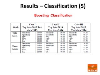
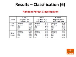
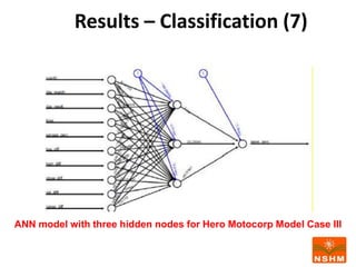
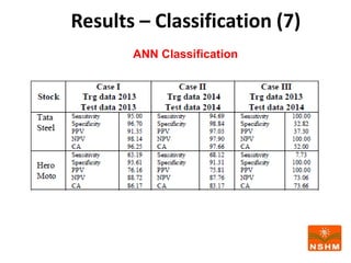
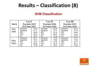
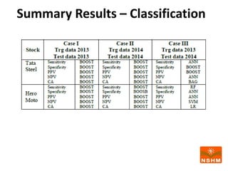
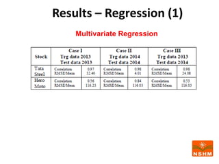
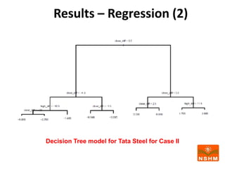
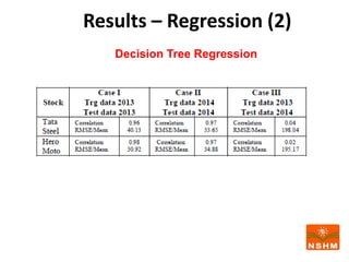
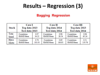
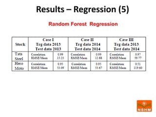
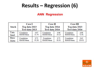
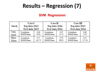
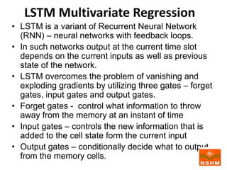
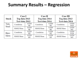
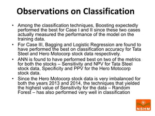
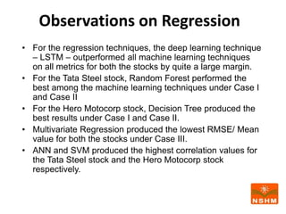
See discussions, stats, and author profiles for this publication at: https://www.researchgate.net/publication/329880659
Stock Price Prediction Using Machine Learning and Deep Learning
Frameworks
Presentation · December 2018
DOI: 10.13140/RG.2.2.35704.49923
CITATIONS
2
READS
3,867
1 author:
Some of the authors of this publication are also working on these related projects:
Internet of Things: Security and Privacy Issues in Applications View project
End-to-End Connectivity Management in Heterogeneous Wireless Networks View project
Jaydip Sen
Praxis Business School
358 PUBLICATIONS   4,371 CITATIONS   
SEE PROFILE
All content following this page was uploaded by Jaydip Sen on 23 December 2018.
The user has requested enhancement of the downloaded file.
Stock Price Prediction Using
Machine Learning and Deep
Learning Frameworks
Jaydip Sen
NSHM College of Management & Technology,
Kolkata, INDIA
6th International Conference on Business Analytics and Intelligence
December 20 - 22, 2018, Bangalore, INDIA
Objective of the Work
• The primary objective of the work is to develop a
robust framework for predicting stock price
movement based on stock price data at 5 minutes
interval of time from the National Stock Exchange
(NSE).
• Our contention is that such a granular approach can
model the inherent dynamics and can be fine-tuned
for immediate forecasting of stock price movement.
Outline
• Related Work
• Methodology
• Results `
Regression
Classification
• Observations on Results
• Conclusion
Related Work
• The literature trying to prove or disprove the efficient
market hypothesis can be classified into three strands.
• The first strand consist of studies using simple
regression techniques on cross sectional data.
• The second strand has used time series models and
techniques to forecast stock returns following
econometric techniques like ARIMA, Granger Causality,
ARDL, etc.
• The third strand includes work using machine learning
and deep learning tools for prediction of stock returns .
Methodology (1)
• We use the Metastock tool for collecting data on stock
price movement of two stocks – Tata Steel and Hero
Motocorp at 5 minutes interval of time over two year
period: January 2013 – December 2014.
• The raw data consisted of the following variables: (i)
date, (ii) time, (iii) open, (iv) high, (v) low, (vi) close,
and (vii) volume.
• We also collected the NIFTY index values
corresponding to each time slot to use it as a market
sentiment variable.
• The total time interval in a day is broken into three
slots and aggregate values of the above variables
are computed for each slot for each day.
 Morning slot: 9:00 AM – 11:30 AM
 Afternoon slot: 11:35 AM – 1:30 PM
 Evening slot: 1:35 PM – till the closure
Methodology (2)
• We derive the following eleven variables for building the predictive
models.
 month
 day_month
 day_week
 time
 open_perc
 sensex_perc
 low_diff
 high_diff
 close_diff
 vol_diff
 range_diff
• open_perc is taken as the response variable and it is predicted using
the values of the other variables as predictors. For regression based
techniques, we predict the value of the open_perc in the next slot
based on predictor values in the previous slots and for classification
techniques we instead of the value, we attempt to predict the
movement (positive or negative) of the open_perc in the next slot.
Methodology (3)
• We applied eight classification techniques
and eight regression techniques for
predicting the stock price values or stock
price movements for two stocks Tata Steel
and Hero Moto Corp.
• Three cases are considered:
 Case I: Model built using 2013 data and tested
on the same data
 Case II: Model built using 2014 data and
tested on the same data
Case III: Model built on 2013 data and tested
on 2014 data.
Results – Classification (1)
Logistic Regression
Results – Classification (2)
KNN Classification
Results – Classification (3)
Decision Tree Classification
Results – Classification (4)
Bagging Classification
Results – Classification (5)
Boosting Classification
Results – Classification (6)
Random Forest Classification
ANN model with three hidden nodes for Hero Motocorp Model Case III
Results – Classification (7)
ANN Classification
Results – Classification (8)
SVM Classification
Summary Results – Classification
Results – Regression (1)
Multivariate Regression
Decision Tree model for Tata Steel for Case II
Results – Regression (2)
Decision Tree Regression
Results – Regression (3)
Bagging Regression
Results – Regression (4)
Boosting Regression
Results – Regression (5)
Random Forest Regression
Results – Regression (6)
ANN Regression
Results – Regression (7)
SVM Regression
LSTM Multivariate Regression
• LSTM is a variant of Recurrent Neural Network
(RNN) – neural networks with feedback loops.
• In such networks output at the current time slot
depends on the current inputs as well as previous
state of the network.
• LSTM overcomes the problem of vanishing and
exploding gradients by utilizing three gates – forget
gates, input gates and output gates.
• Forget gates - control what information to throw
away from the memory at an instant of time
• Input gates – controls the new information that is
added to the cell state form the current input
• Output gates – conditionally decide what to output
from the memory cells.
LSTM Forget Gates
The forget gate takes two
inputs h_t-1 and x_t. h_t-1 is
the hidden state from the
previous cell (i.e., the output
from the previous cell and
x_t is the input at that
particular time step)The
inputs are multiplied by
weight matrices and a bias
is added and the resultant
input is passed through a
sigmoid function. The inputs
for which sigmoid produces
“0” are forgotten.
LSTM Input Gates
The input gates work on three-step
process.
1, Regulating what values need to
be added to the cell state. This is
done by passing h_t-1 and x_t
through a sigmoid function.
2. Creating a vector containing all
possible values that can be added to
the cell state – done using the tanh
function. The function produces
output from -1 to +1.
3. Multiplying the value of the
sigmoid output to the tanh output
and then adding this useful
information to the cell state via an
addition operation
LSTM Output Gates
These gates work in three steps:
1. Creating a vector after
applying tanh function to the cell
state
2. Passing h_t-1 and x_t through
a sigmoid function so that
outputted values may be
regulated
3. Multiplying the results of 1
and 2 and sending it as the
output and also the hidden state
of the next cell
LSTM Implementation Details
• Python Language
• Tensorflow deep learning framework of
Goggle
• Loss function: MAE
• Optimizer: ADAM
• Optimum epoch: 60
• Batch size: 100
• Sequential() function in the Tensorflow
module used for building the LSTM network
Results – Regression (8)
LSTM Regression
Results – Regression (8)
Loss Convergence in LSTM Model (Tata Steel Case III)
(x-axis: no of epochs, y-axis: percentage of loss)
Summary Results – Regression
Observations on Classification
• Among the classification techniques, Boosting expectedly
performed the best for Case I and II since these two cases
actually measured the performance of the model on the
training data.
• For Case III, Bagging and Logistic Regression are found to
have performed the best on classification accuracy for Tata
Steel and Hero Motocorp stock data respectively.
• ANN is found to have performed best on two of the metrics
for both the stocks – Sensitivity and NPV for Tata Steel
stock data, Specificity and PPV for the Hero Motocorp
stock data.
• Since the Hero Motocorp stock data is very imbalanced for
both the years 2013 and 2014, the techniques that yielded
the highest value of Sensitivity for the data – Random
Forest – has also performed very well in classification
Observations on Regression
• For the regression techniques, the deep learning technique
– LSTM – outperformed all machine learning techniques
on all metrics for both the stocks by quite a large margin.
• For the Tata Steel stock, Random Forest performed the
best among the machine learning techniques under Case I
and Case II
• For the Hero Motocorp stock, Decision Tree produced the
best results under Case I and Case II.
• Multivariate Regression produced the lowest RMSE/ Mean
value for both the stocks under Case III.
• ANN and SVM produced the highest correlation values for
the Tata Steel stock and the Hero Motocorp stock
respectively.
Conclusion
• We have presented a framework of predictive models for stock
price movement prediction in a short-term time interval using
machine learning and deep learning approaches.
• We built eight regression and eight classification models and
tested those models on two different stock data for year time
interval – Jan 2013 to Dec 2014.
• Extensive results have been presented on performance of these
models.
• It has been observed that while among the classification
techniques ANN has, on the average, produced the best results,
LSTM outperformed, by a large margin, all other regression
models.
• Identifying the individual error values in regression by LSTM and
studying those errors constitute a future course of work.
References (1)
• Adebiyi A., Adewumi A. O. and Ayo C. K. (2014). Stock price prediction using the ARIMA model.
Proceedings of the International Conference on Computer Modelling and Simulation, Cambridge, UK,
pp. 105-111.
• Basu S. (1983). The relationship between earnings yield, market value and return for NYSE common
stocks: Further Evidence. Journal of Financial Economics, 12(1), 129-156.
• Chui, A. and Wei, K. (1998). Book-to-market, firm size, and the turn of the year effect: Evidence from
Pacific basin emerging markets. Pacific Basin Finance Journal, 6(3-4), 275-293.
• Dutta, G., Jha, P., Laha, A. and Mohan, N. (2006). Artificial neural network models for forecasting
stock price index in the Bombay Stock Exchange. Journal of Emerging Market Finance, 5(3), 283-295.
• Fama, E. F. and French, K. R. (1995). Size and book-to-market factors in earnings and returns. Journal
of Finance, 50(1), 131-155.
• Jaffe J, Keim D. B. and Westerfield R. (1989). Earnings yields, market values, and stock returns. Journal
of Finance, 44, 135-148.
• Jarrett, J. E. and Kyper, E. (2011). ARIMA modeling with intervention to forecast and analyze Chinese
stock prices. International Journal of Engineering Business Management, 3(3), 53-58.
• Jaruszewicz, M. and Mandziuk, J (2004). One day prediction of Nikkei index considering information
from other stock markets. Proceedings of the International Conference on Artificial Intelligence and
Soft Computing, Japan, 1130–1135.
• Metastock Website: https://www.metastock.com.
• Mishra, S. (2016). The quantile regression approach to analysis of dynamic interaction between
exchange rate and stock returns in emerging markets: Case of BRIC nations. IUP Journal of Financial
Risk Management, 13(1),7-27.
References (2)
• Mondal, P, Shit, L. and Goswami, S. (2014). Study of effectiveness of time series modeling (ARIMA) in
forecasting stock prices. International Journal of Computer Science, Engineering and Applications, 4, 13-29.
• Mostafa, M. (2010). Forecasting stock exchange movements using neural networks: Empirical evidence from
Kuwait. Expert Systems with Application, 37, 6302-6309.
• Rosenberg, B., Reid, K. and Lanstein, R. (1985). Persuasive evidence of market inefficiency. Journal of
Portfolio Management, 11, 9-17.
• Sen, J. and Datta Chaudhuri, T. (2016a). An alternative framework for time series decomposition and
forecasting and its relevance for portfolio choice - A comparative study of the Indian consumer durable and
small cap sector. Journal of Economics Library, 3(2), 303 - 326.
• Sen, J. and Datta Chaudhuri, T. (2016b). An investigation of the structural characteristics of the Indian IT
sector and the capital goods sector - An application of the R programming language in time series
decomposition and forecasting. Journal of Insurance and Financial Management, 1(4), 68 - 132.
• Siddiqui, T. A. and Abdullah, Y. (2015). Developing a nonlinear model to predict stock prices in India: An
artificial neural networks approach. IUP Journal of Applied Finance, 21(3), 36-49.
• Wu, Q., Chen, Y. and Liu, Z. (2008). Ensemble model of intelligent paradigms for stock market forecasting.
Proceedings of the IEEE 1st International Workshop on Knowledge Discovery and Data Mining, Washington
DC, USA, pp. 205–208.
• Sen, J. and Datta Chaudhuri, T. (2016). Decomposition of time series data to check consistency between
fund style and actual fund composition of mutual funds. Proceedings of the 4th International Conference on
Business Analytics and Intelligence (ICBAI’2016), Indian Institute of Science, Bangalore, December 19 -21,
2016. DOI: 10.13140/RG2.2.33048.19206
• Sen, J. and Datta Chaudhuri, T. (2017). A robust predictive model for stock price forecasting. Proceedings of
the 5th International Conference on Business Analytics and Intelligence, Indian Institute of Management,
Bangalore, December 11 – 13, 2017.
References (3)
• Sen, J. and Datta Chaudhuri, T. (2015) . A framework for predictive analysis of stock market indices –
a study of the Indian auto sector. Calcutta Business School (CBS) Journal of Management Practices,
Vol 2, No 2, pp. 1 – 20.
• Sen, J. and Datta Chaudhuri, T. (2017). A time-series analysis-based forecasting framework for the
Indian healthcare sector. Journal of Insurance and Financial Management, Vol 3, No 1, pp. 66 – 94.
• Sen, J. and Datta Chaudhuri, T. (2017). A predictive analysis of the Indian FMCG sector using time
series decomposition-based approach. Journal of Economic Library, Vol 4, No 2, pp. 206 – 226. DOI:
http://dx.doi.org/10.1453/jel.v4i2.1282.
• Sen, J. (2017). A time-series analysis-based forecasting approach for the Indian realty sector.
International Journal of Applied Economic Studies, Vol 5, No 4, pp. 8 -27.
• Sen, J. A robust analysis and forecasting framework for the Indian mid cap sector using time series
decomposition. Journal of Insurance and Financial Management, Vol 3, No 4, pp. 1 – 32.
• Sen, J. and Datta Chaudhuri, T. (2018). Understanding the sectors of Indian Economy for portfolio
choice. International Journal of Business Forecasting and Marketing Intelligence, Vol 4, No 2, pp. 178
– 222. DOI: http://dx.doi.org/10.1504/IJBFMI.2018.090914
• Sen, J. (2018). Stock composition of mutual funds and fund style: a time series decomposition
approach towards testing for consistency. International Journal of Business Forecasting and
Marketing Intelligence, Vol 4, No 3, pp. 235 – 292. DOI:
http://dx.doi.org/10.1504/IJBFMI.2018.092781
• Sen, J. and Datta Chaudhuri, T. (2016). Decomposition of time series data of stock markets and its
implications for prediction – an application for the Indian auto sector. Proceedings of the 2nd National
Conference on Advances in Business Research and Management Practices (ABRMP’2016), Kolkata,
India, pp. 15 -28. DOI: 10.13140/RG2.1.3232.0241
Thank You!
View publication stats

Icbai 2018 ver_1

  • 1.
    See discussions, stats,and author profiles for this publication at: https://www.researchgate.net/publication/329880659 Stock Price Prediction Using Machine Learning and Deep Learning Frameworks Presentation · December 2018 DOI: 10.13140/RG.2.2.35704.49923 CITATIONS 2 READS 3,867 1 author: Some of the authors of this publication are also working on these related projects: Internet of Things: Security and Privacy Issues in Applications View project End-to-End Connectivity Management in Heterogeneous Wireless Networks View project Jaydip Sen Praxis Business School 358 PUBLICATIONS   4,371 CITATIONS    SEE PROFILE All content following this page was uploaded by Jaydip Sen on 23 December 2018. The user has requested enhancement of the downloaded file.
  • 2.
    Stock Price PredictionUsing Machine Learning and Deep Learning Frameworks Jaydip Sen NSHM College of Management & Technology, Kolkata, INDIA 6th International Conference on Business Analytics and Intelligence December 20 - 22, 2018, Bangalore, INDIA
  • 3.
    Objective of theWork • The primary objective of the work is to develop a robust framework for predicting stock price movement based on stock price data at 5 minutes interval of time from the National Stock Exchange (NSE). • Our contention is that such a granular approach can model the inherent dynamics and can be fine-tuned for immediate forecasting of stock price movement.
  • 4.
    Outline • Related Work •Methodology • Results ` Regression Classification • Observations on Results • Conclusion
  • 5.
    Related Work • Theliterature trying to prove or disprove the efficient market hypothesis can be classified into three strands. • The first strand consist of studies using simple regression techniques on cross sectional data. • The second strand has used time series models and techniques to forecast stock returns following econometric techniques like ARIMA, Granger Causality, ARDL, etc. • The third strand includes work using machine learning and deep learning tools for prediction of stock returns .
  • 6.
    Methodology (1) • Weuse the Metastock tool for collecting data on stock price movement of two stocks – Tata Steel and Hero Motocorp at 5 minutes interval of time over two year period: January 2013 – December 2014. • The raw data consisted of the following variables: (i) date, (ii) time, (iii) open, (iv) high, (v) low, (vi) close, and (vii) volume. • We also collected the NIFTY index values corresponding to each time slot to use it as a market sentiment variable. • The total time interval in a day is broken into three slots and aggregate values of the above variables are computed for each slot for each day.  Morning slot: 9:00 AM – 11:30 AM  Afternoon slot: 11:35 AM – 1:30 PM  Evening slot: 1:35 PM – till the closure
  • 7.
    Methodology (2) • Wederive the following eleven variables for building the predictive models.  month  day_month  day_week  time  open_perc  sensex_perc  low_diff  high_diff  close_diff  vol_diff  range_diff • open_perc is taken as the response variable and it is predicted using the values of the other variables as predictors. For regression based techniques, we predict the value of the open_perc in the next slot based on predictor values in the previous slots and for classification techniques we instead of the value, we attempt to predict the movement (positive or negative) of the open_perc in the next slot.
  • 8.
    Methodology (3) • Weapplied eight classification techniques and eight regression techniques for predicting the stock price values or stock price movements for two stocks Tata Steel and Hero Moto Corp. • Three cases are considered:  Case I: Model built using 2013 data and tested on the same data  Case II: Model built using 2014 data and tested on the same data Case III: Model built on 2013 data and tested on 2014 data.
  • 9.
    Results – Classification(1) Logistic Regression
  • 10.
    Results – Classification(2) KNN Classification
  • 11.
    Results – Classification(3) Decision Tree Classification
  • 12.
    Results – Classification(4) Bagging Classification
  • 13.
    Results – Classification(5) Boosting Classification
  • 14.
    Results – Classification(6) Random Forest Classification
  • 15.
    ANN model withthree hidden nodes for Hero Motocorp Model Case III Results – Classification (7)
  • 16.
    Results – Classification(7) ANN Classification
  • 17.
    Results – Classification(8) SVM Classification
  • 18.
    Summary Results –Classification
  • 19.
    Results – Regression(1) Multivariate Regression
  • 20.
    Decision Tree modelfor Tata Steel for Case II Results – Regression (2)
  • 21.
    Results – Regression(2) Decision Tree Regression
  • 22.
    Results – Regression(3) Bagging Regression
  • 23.
    Results – Regression(4) Boosting Regression
  • 24.
    Results – Regression(5) Random Forest Regression
  • 25.
    Results – Regression(6) ANN Regression
  • 26.
    Results – Regression(7) SVM Regression
  • 27.
    LSTM Multivariate Regression •LSTM is a variant of Recurrent Neural Network (RNN) – neural networks with feedback loops. • In such networks output at the current time slot depends on the current inputs as well as previous state of the network. • LSTM overcomes the problem of vanishing and exploding gradients by utilizing three gates – forget gates, input gates and output gates. • Forget gates - control what information to throw away from the memory at an instant of time • Input gates – controls the new information that is added to the cell state form the current input • Output gates – conditionally decide what to output from the memory cells.
  • 28.
    LSTM Multivariate Regression •LSTM is a variant of Recurrent Neural Network (RNN) – neural networks with feedback loops. • In such networks output at the current time slot depends on the current inputs as well as previous state of the network. • LSTM overcomes the problem of vanishing and exploding gradients by utilizing three gates – forget gates, input gates and output gates. • Forget gates - control what information to throw away from the memory at an instant of time • Input gates – controls the new information that is added to the cell state form the current input • Output gates – conditionally decide what to output from the memory cells.
  • 29.
    LSTM Forget Gates Theforget gate takes two inputs h_t-1 and x_t. h_t-1 is the hidden state from the previous cell (i.e., the output from the previous cell and x_t is the input at that particular time step)The inputs are multiplied by weight matrices and a bias is added and the resultant input is passed through a sigmoid function. The inputs for which sigmoid produces “0” are forgotten.
  • 30.
    LSTM Input Gates Theinput gates work on three-step process. 1, Regulating what values need to be added to the cell state. This is done by passing h_t-1 and x_t through a sigmoid function. 2. Creating a vector containing all possible values that can be added to the cell state – done using the tanh function. The function produces output from -1 to +1. 3. Multiplying the value of the sigmoid output to the tanh output and then adding this useful information to the cell state via an addition operation
  • 31.
    LSTM Output Gates Thesegates work in three steps: 1. Creating a vector after applying tanh function to the cell state 2. Passing h_t-1 and x_t through a sigmoid function so that outputted values may be regulated 3. Multiplying the results of 1 and 2 and sending it as the output and also the hidden state of the next cell
  • 32.
    LSTM Implementation Details •Python Language • Tensorflow deep learning framework of Goggle • Loss function: MAE • Optimizer: ADAM • Optimum epoch: 60 • Batch size: 100 • Sequential() function in the Tensorflow module used for building the LSTM network
  • 33.
    Results – Regression(8) LSTM Regression
  • 34.
    Results – Regression(8) Loss Convergence in LSTM Model (Tata Steel Case III) (x-axis: no of epochs, y-axis: percentage of loss)
  • 35.
  • 36.
    Observations on Classification •Among the classification techniques, Boosting expectedly performed the best for Case I and II since these two cases actually measured the performance of the model on the training data. • For Case III, Bagging and Logistic Regression are found to have performed the best on classification accuracy for Tata Steel and Hero Motocorp stock data respectively. • ANN is found to have performed best on two of the metrics for both the stocks – Sensitivity and NPV for Tata Steel stock data, Specificity and PPV for the Hero Motocorp stock data. • Since the Hero Motocorp stock data is very imbalanced for both the years 2013 and 2014, the techniques that yielded the highest value of Sensitivity for the data – Random Forest – has also performed very well in classification
  • 37.
    Observations on Regression •For the regression techniques, the deep learning technique – LSTM – outperformed all machine learning techniques on all metrics for both the stocks by quite a large margin. • For the Tata Steel stock, Random Forest performed the best among the machine learning techniques under Case I and Case II • For the Hero Motocorp stock, Decision Tree produced the best results under Case I and Case II. • Multivariate Regression produced the lowest RMSE/ Mean value for both the stocks under Case III. • ANN and SVM produced the highest correlation values for the Tata Steel stock and the Hero Motocorp stock respectively.
  • 38.
    Conclusion • We havepresented a framework of predictive models for stock price movement prediction in a short-term time interval using machine learning and deep learning approaches. • We built eight regression and eight classification models and tested those models on two different stock data for year time interval – Jan 2013 to Dec 2014. • Extensive results have been presented on performance of these models. • It has been observed that while among the classification techniques ANN has, on the average, produced the best results, LSTM outperformed, by a large margin, all other regression models. • Identifying the individual error values in regression by LSTM and studying those errors constitute a future course of work.
  • 39.
    References (1) • AdebiyiA., Adewumi A. O. and Ayo C. K. (2014). Stock price prediction using the ARIMA model. Proceedings of the International Conference on Computer Modelling and Simulation, Cambridge, UK, pp. 105-111. • Basu S. (1983). The relationship between earnings yield, market value and return for NYSE common stocks: Further Evidence. Journal of Financial Economics, 12(1), 129-156. • Chui, A. and Wei, K. (1998). Book-to-market, firm size, and the turn of the year effect: Evidence from Pacific basin emerging markets. Pacific Basin Finance Journal, 6(3-4), 275-293. • Dutta, G., Jha, P., Laha, A. and Mohan, N. (2006). Artificial neural network models for forecasting stock price index in the Bombay Stock Exchange. Journal of Emerging Market Finance, 5(3), 283-295. • Fama, E. F. and French, K. R. (1995). Size and book-to-market factors in earnings and returns. Journal of Finance, 50(1), 131-155. • Jaffe J, Keim D. B. and Westerfield R. (1989). Earnings yields, market values, and stock returns. Journal of Finance, 44, 135-148. • Jarrett, J. E. and Kyper, E. (2011). ARIMA modeling with intervention to forecast and analyze Chinese stock prices. International Journal of Engineering Business Management, 3(3), 53-58. • Jaruszewicz, M. and Mandziuk, J (2004). One day prediction of Nikkei index considering information from other stock markets. Proceedings of the International Conference on Artificial Intelligence and Soft Computing, Japan, 1130–1135. • Metastock Website: https://www.metastock.com. • Mishra, S. (2016). The quantile regression approach to analysis of dynamic interaction between exchange rate and stock returns in emerging markets: Case of BRIC nations. IUP Journal of Financial Risk Management, 13(1),7-27.
  • 40.
    References (2) • Mondal,P, Shit, L. and Goswami, S. (2014). Study of effectiveness of time series modeling (ARIMA) in forecasting stock prices. International Journal of Computer Science, Engineering and Applications, 4, 13-29. • Mostafa, M. (2010). Forecasting stock exchange movements using neural networks: Empirical evidence from Kuwait. Expert Systems with Application, 37, 6302-6309. • Rosenberg, B., Reid, K. and Lanstein, R. (1985). Persuasive evidence of market inefficiency. Journal of Portfolio Management, 11, 9-17. • Sen, J. and Datta Chaudhuri, T. (2016a). An alternative framework for time series decomposition and forecasting and its relevance for portfolio choice - A comparative study of the Indian consumer durable and small cap sector. Journal of Economics Library, 3(2), 303 - 326. • Sen, J. and Datta Chaudhuri, T. (2016b). An investigation of the structural characteristics of the Indian IT sector and the capital goods sector - An application of the R programming language in time series decomposition and forecasting. Journal of Insurance and Financial Management, 1(4), 68 - 132. • Siddiqui, T. A. and Abdullah, Y. (2015). Developing a nonlinear model to predict stock prices in India: An artificial neural networks approach. IUP Journal of Applied Finance, 21(3), 36-49. • Wu, Q., Chen, Y. and Liu, Z. (2008). Ensemble model of intelligent paradigms for stock market forecasting. Proceedings of the IEEE 1st International Workshop on Knowledge Discovery and Data Mining, Washington DC, USA, pp. 205–208. • Sen, J. and Datta Chaudhuri, T. (2016). Decomposition of time series data to check consistency between fund style and actual fund composition of mutual funds. Proceedings of the 4th International Conference on Business Analytics and Intelligence (ICBAI’2016), Indian Institute of Science, Bangalore, December 19 -21, 2016. DOI: 10.13140/RG2.2.33048.19206 • Sen, J. and Datta Chaudhuri, T. (2017). A robust predictive model for stock price forecasting. Proceedings of the 5th International Conference on Business Analytics and Intelligence, Indian Institute of Management, Bangalore, December 11 – 13, 2017.
  • 41.
    References (3) • Sen,J. and Datta Chaudhuri, T. (2015) . A framework for predictive analysis of stock market indices – a study of the Indian auto sector. Calcutta Business School (CBS) Journal of Management Practices, Vol 2, No 2, pp. 1 – 20. • Sen, J. and Datta Chaudhuri, T. (2017). A time-series analysis-based forecasting framework for the Indian healthcare sector. Journal of Insurance and Financial Management, Vol 3, No 1, pp. 66 – 94. • Sen, J. and Datta Chaudhuri, T. (2017). A predictive analysis of the Indian FMCG sector using time series decomposition-based approach. Journal of Economic Library, Vol 4, No 2, pp. 206 – 226. DOI: http://dx.doi.org/10.1453/jel.v4i2.1282. • Sen, J. (2017). A time-series analysis-based forecasting approach for the Indian realty sector. International Journal of Applied Economic Studies, Vol 5, No 4, pp. 8 -27. • Sen, J. A robust analysis and forecasting framework for the Indian mid cap sector using time series decomposition. Journal of Insurance and Financial Management, Vol 3, No 4, pp. 1 – 32. • Sen, J. and Datta Chaudhuri, T. (2018). Understanding the sectors of Indian Economy for portfolio choice. International Journal of Business Forecasting and Marketing Intelligence, Vol 4, No 2, pp. 178 – 222. DOI: http://dx.doi.org/10.1504/IJBFMI.2018.090914 • Sen, J. (2018). Stock composition of mutual funds and fund style: a time series decomposition approach towards testing for consistency. International Journal of Business Forecasting and Marketing Intelligence, Vol 4, No 3, pp. 235 – 292. DOI: http://dx.doi.org/10.1504/IJBFMI.2018.092781 • Sen, J. and Datta Chaudhuri, T. (2016). Decomposition of time series data of stock markets and its implications for prediction – an application for the Indian auto sector. Proceedings of the 2nd National Conference on Advances in Business Research and Management Practices (ABRMP’2016), Kolkata, India, pp. 15 -28. DOI: 10.13140/RG2.1.3232.0241
  • 42.
    Thank You! View publicationstats View publication stats