This dissertation studies synthetic molecular motors and self-assembled monolayers through computational modeling and simulation. Chapter 1 provides background on molecular motors and the theoretical methods used, including density functional theory and classical force fields. Chapter 2 models a caltrop-based rotary motor driven by rotating electric fields, finding resonance effects that enhance friction. Chapter 3 presents a novel power law mechanism for dissipation in motors indirectly coupled to a thermal bath. Chapter 4 models the kinetics of monolayer displacement and finds it follows a universal perimeter-dependent growth model. Chapter 5 provides preliminary results on barriers to rotation in lanthanide double-decker complexes as potential rotary motors.

1. The Pennsylvania State University
The Graduate School
MODELLING OF SYNTHETIC MOLECULAR MOTORS AND
SELF-ASSEMBLED MONOLAYERS
A Dissertation in
Physics
by
Corina Madalina Barbu
c 2008 Corina Madalina Barbu
Submitted in Partial Fulfillment
of the Requirements
for the Degree of
Doctor of Philosophy
December 2008

2. The dissertation of Corina Madalina Barbu was reviewed and approved∗
by the
following:
Vincent H. Crespi
Professor of Physics
Professor of Materials Science and Engineering
Dissertation Advisor, Chair of Committee
Paul Weiss
Distinguished Professor of Physics
Distinguished Professor of Chemistry
Jorge O. Sofo
Associate Professor of Physics
Associate Professor of Materials Science and Engineering
Richard Robinett
Professor of Physics
Jayanth R. Banavar
Distinguished Professor of Physics
George A. and Margaret M. Downsbrough Department Head of Physics
∗
Signatures are on file in the Graduate School.

3. Abstract
The main goals of this dissertation work are the modelling of the static and dynamic
properties and mechanisms of energy dissipation of synthetic molecular motors, as
well as modelling of the kinetics of exchange reaction processes in self-assembled
monolayers.
Chapter 1 presents a brief overview of the field of synthetic molecular motors
and some of the theoretical methods used to evaluate their static and dynamic
properties: density functional theory and universal force field classical potential.
Artificial molecular motors have been created by scientists in order to develop bet-
ter understanding of the biological ones, to mimic and to augment their functions.
We discuss several different types of motors, classified according to the sources of
fuel used as input energy, the environment in which they operate, and the type of
mechanical-like motion they produce.
In chapter 2, we study the static and dynamic properties of a synthetic caltrop-
based rotary molecular motor chemically attached to a surface and driven by ex-
ternal rotational electric fields. Our theoretical calculations and simulations show
that external rotating electric fields with magnitudes accessible experimentally in-
duce unidirectional and repetitive rotation of the dipole-carrying rotator of the
motor. The rotation occurs about the triple bond within the shaft of the motor.
Resonances between the external drive and the soft modes associated with the
deviation of the shaft of the motor with respect to the vertical axis give rise to a
dramatic increase in friction within the motor.
In chapter 3, we present a novel mechanism of dissipation in nanoscale and
molecular-scale motors. We investigate a situation in which one degree of freedom
is pulled out from the thermal bath and given an explicit equation of motion,
interposed between the bath and the motor. We describe a regime in which the
deceleration of an unpowered motor, coupled to a thermal bath via an explicit
degree of freedom, follows a power law in time with universal exponent of t equal
iii

4. to -1, rather than a standard exponential decay. We find that the span of the
power law regime depends only on four dimensionless parameters and it can cover
up to a few hundred elastic collisions between the motor and the damper.
Surfaces self-limited to a single layer of molecules on a substrate, known as
self-assembled monolayers, have important applications in nanotechnology. Ex-
perimental investigations show evidence that n-dodecanethiol molecules in solution
displace 1-adamantanethiolate self-assembled monolayers on Au{111}, leading to
complete molecular exchange. In chapter 4, we attempt to model the kinetics of the
displacement process and we find that it can be described by the Johnson-Mehl-
Avrami-Kolmogorov model of perimeter-dependent island growth for the whole
range of n-dodecanethiol solution concentrations studied. Rescaling the growth
rate at each concentration collapses all the data onto a single universal curve,
suggesting that the displacement is a purely geometrical, scale-free process.
Synthetic rotary motors, consisting of planar organic ligands with metal ions
sandwiched in between, have gained a lot of attention recently. In chapter 5,
we present some preliminary results for barriers to rotation in lanthanide double-
decker complexes. Density functional theory calculations performed on isolated
luthetium double-decker complexes, with no side-substituents added on the ligands,
reveal substantial barriers to rotation. The modulation of the rotational barrier
with size and position of ligand side-substituents, or metal ion, is proposed as a
next step.
iv

5. Table of Contents
List of Figures vii
List of Symbols xii
Acknowledgments xiv
Chapter 1
Introduction 1
1.1 Molecular motors background . . . . . . . . . . . . . . . . . . . . . 1
1.2 Density functional theory . . . . . . . . . . . . . . . . . . . . . . . . 4
1.2.1 Hohenberg-Kohn theorems . . . . . . . . . . . . . . . . . . . 4
1.2.2 Kohn-Sham equations . . . . . . . . . . . . . . . . . . . . . 6
1.2.3 The search for approximate exchange-correlation
functionals . . . . . . . . . . . . . . . . . . . . . . . . . . . . 9
1.3 Universal force field classical potential . . . . . . . . . . . . . . . . 12
Chapter 2
Synthetic caltrop-based molecular motors driven by rotating
electric field 16
2.1 Introduction . . . . . . . . . . . . . . . . . . . . . . . . . . . . . . . 16
2.2 Static properties of the motor with density functional theory . . . . 19
2.3 Static and dynamic properties of the motor with classical molecular
dynamics . . . . . . . . . . . . . . . . . . . . . . . . . . . . . . . . 25
2.3.1 Assessment of quality of UFF classical potential . . . . . . . 25
2.3.2 Vibrational analysis . . . . . . . . . . . . . . . . . . . . . . . 28
2.3.3 Dynamic behavior in external electric field . . . . . . . . . . 31
2.3.4 Field-free decay analysis . . . . . . . . . . . . . . . . . . . . 39
v

6. 2.4 Modelling of the molecular caltrop . . . . . . . . . . . . . . . . . . 42
2.5 Conclusions . . . . . . . . . . . . . . . . . . . . . . . . . . . . . . . 49
Chapter 3
Power law dissipation in motors indirectly coupled to a thermal
bath 50
3.1 Introduction . . . . . . . . . . . . . . . . . . . . . . . . . . . . . . . 50
3.2 Simple geometrical setup . . . . . . . . . . . . . . . . . . . . . . . . 52
3.3 Numerical simulations . . . . . . . . . . . . . . . . . . . . . . . . . 55
3.4 Power law regime span . . . . . . . . . . . . . . . . . . . . . . . . . 58
3.5 Physical systems . . . . . . . . . . . . . . . . . . . . . . . . . . . . 61
3.6 Conclusions . . . . . . . . . . . . . . . . . . . . . . . . . . . . . . . 62
Chapter 4
1-Adamantanethiolate monolayer displacement kinetics follow a
universal form 64
4.1 Introduction . . . . . . . . . . . . . . . . . . . . . . . . . . . . . . . 64
4.2 Experimental results . . . . . . . . . . . . . . . . . . . . . . . . . . 66
4.3 Modelling of the kinetics of the displacement process . . . . . . . . 69
4.4 Conclusions . . . . . . . . . . . . . . . . . . . . . . . . . . . . . . . 76
Chapter 5
Lanthanide double-decker complexes as potential rotary motors 77
5.1 Introduction . . . . . . . . . . . . . . . . . . . . . . . . . . . . . . . 77
5.2 Barriers to rotation for lanthanide DD
complexes using DFT . . . . . . . . . . . . . . . . . . . . . . . . . . 78
5.3 Conclusions . . . . . . . . . . . . . . . . . . . . . . . . . . . . . . . 81
Bibliography 82
vi

7. List of Figures
2.1 Synthetic caltrop-based rotary molecular motor is attached to sur-
faces and driven by rotational electric fields. The motor contains a
rotor on top, a shaft in the middle and a three-legged base. The col-
ors of the atoms in the structure are as follows: carbon-dark blue,
hydrogen-green, nitrogen-light blue, oxygen-red, silicon-violet and
sulfur-yellow. . . . . . . . . . . . . . . . . . . . . . . . . . . . . . . 18
2.2 Electrostatic potential energy of a 12.5 Debye permanent dipole mo-
ment in an external electric field of 0.5 V
nm
as a function of the angle
between the field and the dipole. The red dashed line represents the
sinusoidal fit to the electrostatic potential energy of the dipole in
electric field. The black dashed line is the thermal energy at room
temperature. . . . . . . . . . . . . . . . . . . . . . . . . . . . . . . . 20
2.3 Barrier to rotation for the middle bond as a function of the relative
angle between the two benzene rings of the shaft of the motor. The
barrier is small and allows rapid thermally activated rotations about
this bond. The black dashed line is the thermal energy at room
temperature. . . . . . . . . . . . . . . . . . . . . . . . . . . . . . . . 21
2.4 The barrier to rotation for the upper bond as a function of the
relative angle between the rotor and the uppermost ring of the shaft
of the motor. The strong interactions between the hydrogen atoms
across the bond give rise to a substantial barrier against rotation.
The black dashed line is the thermal energy at room temperature. . 22
2.5 The relaxed (black solid line) and unrelaxed (red dashed line) bar-
riers to rotation obtained by rotating the upper ring of the caltrop
structure with respect to the other three. The barrier is fluctuat-
ing and allows intermittent rotation. The black dashed line is the
thermal energy at room temperature. . . . . . . . . . . . . . . . . . 23
2.6 Barrier to rotation about the single N–C bond between the rotor
and the upper phenyl ring of the shaft using DFT (black line) and
UFF (red line). . . . . . . . . . . . . . . . . . . . . . . . . . . . . . 26
vii

8. 2.7 Barrier to rotation about the triple bond within the shaft of the
motor using DFT (black line) and UFF (red line). . . . . . . . . . . 26
2.8 Schematic representation of the wobbling modes of the motor with
characteristic frequencies of 50 and 80 GHz. The mode corresponds
to an oscillation of the motor shaft with respect to the vertical axis. 29
2.9 Schematic representation of the seesaw-like mode of the motor with
characteristic frequency of 193 GHz. The mode corresponds to an
oscillation of the rotor axis about the horizontal plane where the
external electric field resides. . . . . . . . . . . . . . . . . . . . . . . 30
2.10 The work per cycle done by the electric field on the motor shows
a broad, asymmetric peak centered at driving frequencies of 70-90
GHz. The magnitudes for the electric field used are: E=2.5 V
nm
(black line) and E=0.5 V
nm
(red line). . . . . . . . . . . . . . . . . . 33
2.11 The work per unit of time done by the electric field on the motor
shows a broad, asymmetric peak centered at driving frequencies of
70-90 GHz. The magnitudes for the electric field used are: E=2.5
V
nm
(black line) and E=0.5 V
nm
(red line). . . . . . . . . . . . . . . . 34
2.12 The average offset angle between the direction of the rotating elec-
tric field and the dipole increases substantially when the motor is
driven at frequencies of 70-90 GHz. The magnitudes for the electric
field used are: E=2.5 V
nm
(black line) and E=0.5 V
nm
(red line). . . . 36
2.13 The average deviation of the shaft of the motor with respect to
the vertical axis increases substantially when the motor is driven at
frequencies of 70-90 GHz. The magnitudes for the electric field used
are: E=2.5 V
nm
(black line) and E=0.5 V
nm
(red line). . . . . . . . . . 37
2.14 Movie snapshots illustrating the dynamical behavior of the motor
when driven at (a) 75 GHz, and (b) 150 GHz, respectively. Field
magnitude equals 2.5 V
nm
. At resonance, the shaft of the motor
undergoes large amplitude motions, causing the rotor to sweep the
substrate underneath. . . . . . . . . . . . . . . . . . . . . . . . . . . 38
2.15 Plots of log (L(t)
L(0)
) versus time (black) and the corresponding linear
fits (red line) for two different initial rotational excitations: (a) 30
GHz (τ=47.5 ps) and (b) 150 GHz (τ=41 ps). . . . . . . . . . . . . 40
2.16 The molecular caltrop consists of four identical phenyl rings con-
nected to a central silicon atom. The structure might function as a
molecular gear if the rotary power generated by mechanically driv-
ing one ring would get transmitted to the other rings via concerted
rotations. . . . . . . . . . . . . . . . . . . . . . . . . . . . . . . . . 41
viii

9. 2.17 The four mutually interacting phenyl rings within the molecular
caltrop can be viewed as a sum of six different pairs of two mutually
interacting phenyl rings. . . . . . . . . . . . . . . . . . . . . . . . . 43
2.18 Family of unrelaxed curves for the two-ring structure obtained by
keeping one dihedral angle at a constant value while varying the
other between 0◦
and 180◦
. The curves can be identified according
to the value of the dihedral angle kept fixed. . . . . . . . . . . . . . 44
2.19 Comparison between the DFT data (black lines) and the analytical
model (blue lines) for the unrelaxed (a) and the relaxed (b) barriers
against rotation of the four-ring structure. . . . . . . . . . . . . . . 46
2.20 Variation of the dihedral angles corresponding to the three lower
phenyl rings of the molecular caltrop (red, green and blue lines)
while the upper phenyl ring (black line) rotates every 10◦
for a total
of 180◦
. . . . . . . . . . . . . . . . . . . . . . . . . . . . . . . . . . 48
3.1 The motor and the damper are constrained to move along linear
tracks that make a small angle φ between them. They undergo
periodic linear head-on collisions at the intersection of their tracks.
The damper always comes back to rest before a new collision with
the motor occurs. . . . . . . . . . . . . . . . . . . . . . . . . . . . 52
3.2 (a) Motor (blue) approaches damper (red) from the left. Damper
is at rest before a collision with the motor occurs. (b) Motor and
damper interact a single time, i.e., at the point of intersection of
their linear tracks. The motor has a high initial velocity, such that
its collision with the damper is strong, and the damper moves out
of the way of the motor rapidly, after the first collision. . . . . . . . 53
3.3 Logarithmic plot for the motor linear momentum in units of its ini-
tial linear momentum, p0, versus time in units of the time constant
of the damper, τd, for α = 125, φ = 5◦
, ξ = 0.8 and L
σ
= 104
. . . . . 56
3.4 Plot of the fraction of the linear momentum that the motor gives
up at each collision with the damper versus time in units of τd, for
α = 125, φ = 5◦
, ξ = 0.8 and L
σ
= 104
. . . . . . . . . . . . . . . . . . 57
3.5 Motor (blue) and damper (red) interact multiple times beyond the
point of intersection of their linear tracks. As the motor slows down
and its collision with the damper weakens, the damper does not
have time to move out of the way of the motor after the first collision. 58
3.6 The contour plots show the numbers of elastic collisions in the power
law regime for α = 125, φ = 5◦
, 0 < ξ < 2 and 250 < L
σ
< 104
.
Notice that the largest number of collisions is obtained for very large
values of L
σ
and ξ close to 1. . . . . . . . . . . . . . . . . . . . . . . 61
ix

10. 3.7 The outer tube (i.e., the motor) oscillates along its axis relative to
the inner tube and loses momentum via linear and periodic collisions
with a small damper. The damper is directly coupled to the thermal
bath (i. e., the inner tube), where it dissipates the energy gained
from the motor. . . . . . . . . . . . . . . . . . . . . . . . . . . . . 62
4.1 A) Schematic representation of the displacement of AD molecules
by C12 molecules. n-dodecanethiolate (C12) molecules insert at
defect sites of the AD SAM during a rapid nucleation phase. B)
STM image of the real process: the (C12) islands grow radially
into domains that coalesce and eventually fully displace the original
monolayer. . . . . . . . . . . . . . . . . . . . . . . . . . . . . . . . . 66
4.2 Infrared spectra of the C-H stretch region of a AD SAM (black)
and a C12 SAM (grey), showing their spectral overlap. . . . . . . . 67
4.3 A) Representative FTIR spectra of a 0.11 mM C12 solution displac-
ing an AD SAM. The 2877 cm−1
peak, corresponding to the CH3
symmetric mode, is highlighted. B) A kinetic curve derived from
the FTIR spectra by plotting the integrated C12 CH3 symmetric
mode peak versus deposition exposure time. The open squares rep-
resent the integrated absorbance for each of the four spectra shown
on the left. . . . . . . . . . . . . . . . . . . . . . . . . . . . . . . . . 68
4.4 A representative 0.01 mM C12 uptake curve with least-squares fits
to pure diffusion (green), first-order Langmuir (purple), first-order
Langmuir with an onset of growth at 23 min (orange), diffusion-
limited Langmuir (grey), second-order Langmuir (black), site-saturated
nucleation JMAK2 (red), and constant-rate nucleation JMAK3 (blue)
models. . . . . . . . . . . . . . . . . . . . . . . . . . . . . . . . . . 73
4.5 n-Dodecanethiolate monolayer formation by the displacement of an
AD SAM as a function of concentration. Solid lines are least-
squares fits based on the site-saturated nucleation model JMAK2
(Eqn. (4.8) with n=2). . . . . . . . . . . . . . . . . . . . . . . . . . 73
4.6 The displacement rate constant versus C12 concentration on a loga-
rithmic scale. The slope of 0.50±0.05 implies that the rate constant
is proportional to the square-root of the C12 concentration. . . . . 74
4.7 A plot of coverage versus reduced exposure time of two experimental
runs at each C12 concentration (0.01, 0.03, 0.11, 0.33, 0.55, 0.77 and
1.0 mM), showing collapse onto a universal curve. . . . . . . . . . . 75
x

11. 5.1 Schematic representation of a double-decker rotary motor consisting
of a Lu ion sandwiched between two Pc ligands. The metal ion plays
the role of the motor shaft, while the upper and the lower ligands
represent the rotor and the stator, respectively. . . . . . . . . . . . 79
5.2 Schematic representation of a double-decker rotary motor consisting
of a Lu ion sandwiched between a Pr ligand (upper) and a Nc ligand
(lower). The metal ion plays the role of the motor shaft, while
the upper and the lower ligands represent the rotor and the stator,
respectively. . . . . . . . . . . . . . . . . . . . . . . . . . . . . . . . 79
5.3 Staggered conformation of optimized (Pr)Lu(Pc) double-decker com-
plex using DFT. (a) Side view. (b) Top view. Atom colors are as
follows: Lu yellow, N blue, C and H green. . . . . . . . . . . . . . . 80
5.4 Staggered conformation of optimized (Pc)Lu(Pc) double-decker com-
plex using DFT. (a) Side view. (b) Top view. Atom colors are as
follows: Lu yellow, N blue, C and H green. . . . . . . . . . . . . . . 81
xi

12. List of Symbols
DFT Density functional theory
LDA Local density approximation
GGA Generalized gradient approximation
B3LYP Hybrid exchange-correlation functional
TZV Triple-split valence basis function
CMD Classical molecular dynamics
UFF Universal force field classical potential
PES Potential energy surface
TINK CMD package using UFF
GAMESS General atomic and molecular electronic system
DWCN Double-walled carbon nanotube
SAM Self-assembled monolayer
ALK Alkane molecule
C12 n-Dodecanethiolate molecule
AD Adamantane molecule
FTIR Fourier transform infrared spectrometry
JMAK Johnson-Mehl-Avrami-Kolmogorov model
xii

13. Pr Porphyrin molecule
Pc Phthalocyanine molecule
Nc Naphthalocyanine molecule
DD Double-decker molecule
(Pr)Lu(Pc) Luthetium Pr/Pc DD complex
(Pr)Lu(Nc) Luthetium Pr/Nc DD complex
(Pc)Lu(Pc) Luthetium Pc/Pc DD complex
(Pc)Lu(Nc) Luthetium Pc/Nc DD complex
xiii

14. Acknowledgments
I would like to begin by thanking my advisor, Prof. Vincent Crespi, for the guid-
ance and patience that he has shown during my time at Penn State and for giving
me the chance to work in his research group. Part of the work in this thesis was
done in collaboration with Prof. Paul Weiss. I am very grateful to him and his
group member, H´ector Miguel Saavedra Garcia, for sharing their experimental
data with me. I owe special thanks to Prof. Jorge Sofo for his helpful discussions
and advice and for always being there when I needed his help. I would also like to
thank Prof. Josef Michl and Prof. Jaroslav Vacek from Colorado State University
for giving me access to the TINK molecular dynamics package and for the warm
hospitality during my visit there. I warmly thank Dr. Paul Lammert for helpful
discussions during my Ph.D. I also want to thank my group members, my family
and my friends. Multumesc mult la toata familia mea de matze.
xiv

15. Dedication
To E. I.
xv

16. Chapter 1
Introduction
1.1 Molecular motors background
Molecular motors are molecular-scale machines that can convert different types of
input energy into mechanical energy, which is further used to perform useful work.
The fundamental difference between the macroscopic motors and the molecular-
scale ones is that the latter operate in an environment that is governed by thermal
fluctuations and they cannot move deterministically.
Nature first constructed tiny and elegant mechanical-like devices that use chem-
ical energy in order to perform numerous functions within cells, such as cell division
or intracellular transport. Although they operate in a world where Brownian mo-
tion and viscous forces dominate, biological motors are capable of achieving highly
controlled rotary and translational motion. For example, ATP-synthase is a rotary
motor that synthesizes the molecule adenosine triphosphate (ATP), which is the
energy currency within cells [1]. The motor rotates with discrete steps of 120◦
and generates a constant force of 40 pN, the highest value among reported mo-
tor proteins. The work done in one-third of a revolution is about 80 pN · nm or
just 20 times larger than thermal energy [2]. Cells also employ a variety of linear
motors that move along and exert forces on filamentous structures. For example,
kinesins and dyneins transport cargo along microtubules and myosins slide on actin
filaments generating forces up to 5-10 pN [3].
Inspired by biological motors, people started designing artificial molecular mo-
tors in attempts to understand and to augment basic motor functions.

17. 2
Artificial molecular motors can be classified according to the input energy they
use, the environment where they operate, or the type of mechanical motion they
produce. They use sources of energy such as: chemical, thermal, gas or liquid
flow, light, electric fields, etc. in order to produce linear or rotary mechanical-like
motion. The motors can operate immersed in liquids or gases, buried in solids, or
chemically attached to surfaces. The disadvantage of liquid and gas environments
is that the gas or liquid non-motor molecules apply viscous forces to the motor,
perturbing its intended function. Because in such enviroments there is no solid
stationary interface nearby for the motor to attach, the motor molecule moves as
a whole and it becomes harder to control the relative motion of its components
and to produce net useful work. By firmly attaching the whole motor to a solid
or a surface, the translational and rotational degrees of freedom associated with
the bulk motion of the motor are suppressed and the positional displacement of
submolecular components becomes the source for generating useful work. On the
other hand, motors buried inside solids or attached to grids and surfaces are at
risk for high dissipation due to coupling between the external drive and different
modes of the solid or substrate.
Kelly et al. [4] reported in 1999 a first example of a synthetic chemically driven
rotary molecular motor capable of performing unidirectional 120◦
rotation. How-
ever, because the sequence of reactions that leads to the initial 120◦
rotation is not
repeatable, the motor did not satisfy one of the basic requirements for a rotary
motor: achievement of repetitive motion. Another example of molecular machines
that can be manipulated by chemical inputs is the family of rotaxane molecules.
They consist of a dumbbell-shaped molecule interlocked with a ring that can travel
along it. Because of their architecture, rotaxanes have potential for applications
in molecular electronics [5], as switching devices [6], or as molecular shuttles [7].
Feringa used light to produce electronic excitation and to induce unidirectional
rotation in a motor that had a high ground-state barrier against rotation [8,9]. The
Feringa motor is much slower [10] in comparison to the rotation speeds displayed
by motor proteins (for example, the rotary bacterial flagellar motor rotates at
speeds of over 100 Hz). Light-driven reversible nanoswitches based on azobenzene
molecules, with potential applications in molecular electronics, as artificial muscles
or molecular motors, have been studied by the Paul Weiss lab [11].

18. 3
Electric fields from scanning tunneling microscope (STM) tips or generated
by applying voltage between nanoelectrodes, have also been used to induce con-
trolled mechanical-like motion in molecules. Coupling to the external drive is
commonly achieved by designing molecules with built-in dipole moments. For
example, electric-field-controlled conformational switches have been constructed
to function as switchable molecular junctions for use in molecular electronics [12].
We discuss a few theoretical and experimental studies of synthetic molecular rotors
chemically attached to surfaces and driven by external electric fields in the intro-
ductory part of Chapter 2. Scanning tunneling microscope tips can also be used
for mechanical manipulation of molecular structures on surfaces. One remarkable
example is the world’s first molecular car [13], which achieved translational motion
and pivoting across a gold surface under the influence of a STM tip. Also, control
of the molecular orientation of double-decker complexes comprised of rare-earth
metals sandwiched between planar ligants on graphite surfaces has been demon-
strated at Penn State [14]. These double-decker complexes are intended for future
applications as molecular rotors attached to surfaces that can be driven by STM
tips, rotating electric fields, or molecular recognition.
Crystalline molecular machines represent another branch of molecular ma-
chines with important applications in nanotechnology. The crystals are built using
molecules that are structurally programmed to respond collectively to external
mechanic, electric, magnetic, or photonic stimuli, in order to fulfill specific func-
tions. M. Garcia-Garibay has studied the dynamics of several different molecular
rotors embedded in carefully engineered molecular crystals and reported rotational
frequencies that range from a few hertz to the gigahertz regime at room tempera-
ture [15]. Possible technological applications target molecular compasses and gyro-
scopes with built-in dipole moments [16] and amphidynamic crystals (i.e., crystals
consisting of solid, rigid frames and highly mobile elements attached to them, such
that the structure displays both phase order and mobility at the same time) [17].
Beams of noble gases have been used by Vacek et al. [18] in a molecular dynam-
ics simulation study, to drive molecular propellers at rotational frequencies of up
to 20-40 GHz. The excitement of rotational motion through momentum transfer
from the gas atoms competed with the induction of pendulum-like motion of the
shaft of the rotary motor, suggesting the need for designing more rigid shafts.

19. 4
However challenging it is to build the molecular-scale machines, it is even more
difficult to control their individual or collective motion. Although artificial molec-
ular motors are still far less complex and efficient than biological motors, much
progress is made every year.
The tools used to investigate the performance of molecular motors can be both
experimental and theoretical. Although a large variety of spectroscopic and micro-
scopic techniques are available today, the experiments are often hard or can exceed
present technological capabilities. Under such conditions, the development of man-
made molecular motors can benefit from theoretical and computational guidance.
We dedicate the remainder of this chapter to the description of the theoretical and
computational techniques used in this thesis: density functional theory used for
quantum mechanical calculations and universal force field classical potential used
for classical molecular dynamics simulations.
1.2 Density functional theory
1.2.1 Hohenberg-Kohn theorems
The mathematical description of a molecular system comprised of M nuclei and N
electrons at a quantum mechanical level is provided by the solution of the many-
body, time-independent, non-relativistic Schr¨odinger equation. This equation can
be simplified if one takes advantage of the huge differences between the masses of
the nuclei and electrons (for example, mass ratio between a proton and an electron
equals roughly 1800.) Since the nuclei move much shower in comparison to the
electrons, one can consider to a good approximation, that the electrons move
in the field of fixed nuclei. This approximation, called the Born-Oppenheimer
approximation, reduces the general Schr¨odinger equation to one of a system of N
electrons in the external field created by stationary nuclei:
ˆHΨ = ˆT + ˆVNe + ˆVee Ψ = EΨ. (1.1)
ˆH is the electronic Hamiltonian, Ψ is the electronic wavefunction, which de-

20. 5
pends explicitly on the coordinates of the electrons while the coordinates of the
nuclei enter only parametrically, and E is the energy. Also, ˆT, ˆVee and ˆVNe are
the operators describing the kinetic energy of the electrons, the electron-electron
interaction energy and the electron-nuclei interaction energy terms, respectively.
Since the equation still proves too complex for any practical use, a series of ad-
ditional approximations for the energy terms in the electronic Hamiltonian above
are necessary in order to solve it. Based on the choice of the approximation, sev-
eral different methods have been developed, such as ab-initio, semiempirical or
molecular mechanics.
In 1964, a revolutionary approach was developed by Hohenberg, Kohn, and
Sham. Instead of attempting to solve for the many-body wave function of the
Schr¨odinger Eqn. (1.1) in order to find information about the system, they pro-
posed that the complete description of the system can be provided via the ground
state charge density, ρ0(r). This approach results in a dramatic simplification of
the problem by transitioning from the need to know 3N degrees of freedom to solve
for the electronic wavefunction, corresponding to the positions of the N electrons
in the system, to just 3 degrees of freedom for the ground state charge density,
ρ0(r).
Density functional theory (DFT) is based on two theorems of Hohenberg and
Kohn [19]. The first one states that the electron density uniquely determines the
Hamilton operator and thus all properties of the system: ‘the external potential
V ext
(r) is (to within a constant) a unique functional of ρ0; since, in turn V ext
(r)
fixes ˆH, we see that the full many particle ground state is a unique functional of
ρ0’. For our case, V ext
(r) is the potential created by the stationary nuclei, ˆVNe in
Eqn. (1.1). The total energy can be now written as a functional of the electronic
density as follows:
E[ρ] = T[ρ] + Eee[ρ] + V ext
(r)ρ(r)dr = FHK[ρ(r)] + V ext
(r)ρ(r)dr. (1.2)
In Eqn. (1.2) above, the energy components have been separated into those
that depend on the specific system, i.e., ENe[ρ] = V ext
(r)ρ(r)dr, the potential
energy due to the nuclei-electron attraction, and those that are not dependent

21. 6
on the number of electrons and nuclei, and the position and charge of the nuclei,
FHK[ρ(r)]. The Hohenberg-Kohn functional, FHK[ρ(r)], contains the electronic
kinetic energy and the electronic Coulomb interaction and is universal by con-
struction. The first Hohenberg-Kohn theorem only claims the existence of a total
energy functional, E[ρ], but it does not provide the means to solve for the ground
state density that delivers the ground state energy.
The second Hohenberg-Kohn theorem states that FHK[ρ(r)], the functional
that delivers the ground state energy of the system, delivers the lowest energy if
and only if the input density is the true ground state density, ρ0. Therefore, for
any given trial density, the true ground state energy, E[ρ0], satisfies the following
relationship: E[ρ0] ≤ E[ρ]. The ground state energy is obtained by minimization
of the energy functional with respect to electron density. In order to have access
to the exact ground state density and energy, one would need to know the form of
the Hohenberg-Kohn functional, FHK[ρ(r)].
There is a restriction for possible densities to be eligible in the variational
procedure of the second Hohenberg-Kohn theorem: there must exist an external
potential associated with the density of choice, since the energy functional E[ρ] is
only defined for ground state densities for which such an external potential exists.
This is known as the V -representability problem, and many possible trial densities
are known not to be V -representable.
The problem of V -representability for eligible densities can be solved using the
Levy constrained formalism [20], in which only so called N-representability of the
trial densities is required. According to the Levy constrained formalism, a trial
density is N-representable if it satisfies the following conditions: is a non-negative
and finite function, ρ(r) ≥ 0, and it integrates to the total number of electrons,
ρ(r)dr = N.
1.2.2 Kohn-Sham equations
The Hohenberg-Kohn theorems presented in subsection 1.2.1 do not provide any
guidance as to how to construct the Hohenberg-Kohn functional, FHK[ρ(r)].
The breakthrough idea that Kohn and Sham [21] proposed was to replace the
system of interacting electrons with one of fictitious, non-interacting particles that

22. 7
has the ground state density of the original one. This way, the many-body wave-
function of the system could be expressed by an antisymmetrized product of N
one-electron wavefunctions, also known as a Slater determinant, ΘS:
ΘS =
1
√
N!
φ1(r1) φ2(r1) ... φN (r1)
φ1(r2) φ2(r2) ... φN (r2)
...
...
...
φ1(rN ) φ2(rN ) ... φN (rN )
The one-particle orbitals, φi(r), are the eigenfunctions of the one-electron
Hamiltonian:
ˆHKS
φi = iφi. (1.3)
The one-electron operator, ˆHKS
, is defined by the following relationship:
ˆHKS
= −
1
2
2
+ Veff(r), (1.4)
with Veff, the effective potential, chosen such that the total density for the system
of fictitious, non-interacting particles equals exactly the ground state density for
the system of real, interacting electrons:
N
i s
|φi(r, s)|2
= ρ0(r), (1.5)
s in the above equation stands for the spin of the electrons.
In light of the new artificial system, the energy functional, F[ρ], that has been
introduced in the previous subsection, can be further partitioned into three parts:
F[ρ] = T0[ρ] + EH[ρ] + Exc[ρ]. (1.6)
T0[ρ] represents the kinetic energy of a non-interacting electron gas:
T0[ρ] = −
1
2
N
i
φi
2
φi . (1.7)
EH[ρ] is the classical electrostatic Coulomb interaction between electrons:

23. 8
EH[ρ] =
1
2
ρ(r)ρ(r )
|r − r |
drdr . (1.8)
Finally, Exc[ρ] is the so-called exchange-correlation energy:
Exc[ρ] ≡ {T[ρ] + Vee[ρ]} − {T0[ρ] + EH[ρ]} . (1.9)
The exchange-correlation energy term, Exc, contains the non-classical effects of
exchange (i.e., electrons of like spin do not move independently from each other)
and correlation and a part of the kinetic energy. The non-interacting kinetic energy,
T0, is not equal to the real kinetic energy of the interacting system, T, even for
the case when the two systems have the same density. The goal of this energy
partition was to separate the energy into terms that can be easily evaluated, T0[ρ]
and EH[ρ], from the ones that cannot, Exc[ρ].
By rewriting the Hohenberg-Kohn expression for the total energy of the inter-
acting system, given by the Eqn. (1.2), using the Kohn-Sham approach described
by the Eqn. (1.6), one obtains:
E[ρ] = T0[ρ] + EH[ρ] + Exc[ρ] + ENe[ρ]
= T0[ρ] +
1
2
ρ(r)ρ(r )
|r − r |
drdr + Exc[ρ] + VNe(r)ρ(r)dr
= −
1
2
N
i
φi
2
φi +
1
2
N
i
N
j
|φi(r)|2 1
|r − r |
|φj(r )|
2
drdr
+Exc[ρ] −
N
i
M
A
ZA
|r − rA|
|φi(r)|2
dr. (1.10)
Because E is expressed as a function of the orbitals, φi, it can be minimized with
respect to them, while keeping the constraint that φi|φj = δij. The equations
obtained further are known as the one-particle Kohn-Sham equations:
−
1
2
2
+
ρ(r )
|r − r |
dr + Vxc(r) −
M
A
ZA
|r − rA|
φi

24. 9
= −
1
2
2
+ Veff (r) φi = iφi (1.11)
By comparing the Kohn-Sham Eqn. (1.11), with the one-particle equations of
the non-interacting auxiliary system, Eqn. (1.3), one obtains the expression for
the Kohn-Sham potential:
Veff (r) =
ρ(r )
|r − r |
dr + Vxc(r) −
M
A
ZA
|r − rA|
. (1.12)
Notice that Veff itself is a function of the electron density. Therefore, the Kohn-
Sham one-electron equations need to be solved iteratively until self-consistency is
achieved. To summarize, by knowing Veff , one can use the one-particle Kohn-
Sham Eqn. (1.11), to determine the orbitals and further, the ground state density,
Eqn. (1.5), and the ground state energy of the electronic system, Eqn. (1.10).
The Kohn-Sham orbitals are the eigenstates of the auxiliary Hamiltonian for
the system of fictitious, non-interacting particles. Thus, they have no physical
meaning; they are not the wavefunctions for the electrons of the real system.
However, they can be used for the qualitative interpretation of the orbitals in a
molecular system or crystal. Also, the eigenvalues associated to the Kohn-Sham
orbitals have no physical meaning, with one exception: the eigenvalue for the
highest occupied molecular orbital equals the negative of the ionization energy.
1.2.3 The search for approximate exchange-correlation
functionals
Up to this point, the Kohn-Sham approach to solving the many-body Schr¨odinger
equation has been exact. Since the form of the exchange-correlation energy func-
tional, Exc[ρ], is unknown, different approximations are made in order to evaluate
it.
Unfortunately, there is no straightforward way in which the exchange-correlation
energy functional can be systematically improved.
For a homogeneous electron gas or an electron gas with slow-varying charge
density, the exchange-correlation energy functional, Exc, can be approximated as:

25. 10
ELDA
xc [ρ(r)] = xc(ρ(r)) ρ(r) dr, (1.13)
with xc the exchange-correlation energy density function. This approximation is
known as the Local Density Approximation (LDA), and it relies on the assumption
that the exchange-correlation energy depends only on the local value of the charge
density. The exchange-correlation energy per electron of a uniform electron gas of
density ρ(r), xc(ρ(r)), can be split into exchange and correlation contributions as
follows:
xc(ρ(r)) = x(ρ(r)) + c(ρ(r)). (1.14)
The exchange contribution, x(ρ(r)), has the following expression:
x(ρ(r)) = −
3
4
3ρ(r)
π
1
3
. (1.15)
For the correlation contribution, c(ρ(r)), several analytical expressions have
been proposed, based on numerical quantum Monte-Carlo simulations [22].
The LDA approximation works well for solid-state systems, but it fails for
most chemical applications, since molecular systems do not satisfy the restriction
of slow-varying electron density. If the spin densities are used as an input to the
energy functional, instead of the total electron density, ρ(r), the approximation is
known as the Local Spin-Density Approximation (LSD).
Better results are obtained if one takes into account not only the electron den-
sity, ρ(r), but also the gradient of the density, ρ(r), which accounts for the non-
homogeneity of the electron density. The exchange-correlation functionals which
include the gradients of the charge density are known as Generalized Gradient
Approximations (GGA). They can be written generically as:
EGGA
xc [ρ(r)] = xc (ρ(r), | ρ(r)|) ρ(r) dr. (1.16)

26. 11
One of the most popular GGA functional is the Becke exchange functional [23]:
EB88
x [ρ(r)] = βy2
1+6βy sinh−1
[y]
(1.17)
where y = | ρ(r)|
ρ(r)4/3 and the empirical parameter β equals 0.0042.
The gradient-corrected correlation functionals have more complicated analyt-
ical forms and, as with the exchange functionals, contain empirical parameters
fitted to reproduce correlation energies of certain atoms. One popular correlation
functional is the LYP functional, proposed by Lee, Yang and Parr in 1988 [24].
Although, in general, the GGA performs better than LDA, the value of a GGA
functional at a specific point in space still depends only on information about
charge density and its gradient at that very point. Therefore, both approximations
presented above neglect the non-local effects that are very important in some
molecular structures where electrons are delocalized, such as aromatic systems.
The hybrid exchange-correlation functionals have proven very successful in ac-
counting for non-local effects. They include pure exchange and correlation func-
tionals determined within the DFT theory, plus another term which corresponds
to a non-local exact exchange functional determined within the ab-initio Hartree-
Fock approximation (HF). The B3LYP functional [25] is the most used hybrid
functional and consists of a combination of the LSD exchange and correlation
functionals, Becke exchange functional, LYP correlation functional and the exact
HF exchange functional.
Hybrid functionals predict molecular geometries substantially better than LDA
and GGA. For example, for organic molecules, bond lengths computed using
B3LYP show an average deviation from experiment of less than 0.01 ˚A and bond
angles are accurate to within a few tenths of a degree.
Also, with B3LYP functional, the errors in the atomization and the ionization en-
ergies are accurate to within 0.1 eV and 0.2 eV, respectively. The errors in dipole
moments calculated using B3LYP are within 0.04 Debye [26].

27. 12
1.3 Universal force field classical potential
As we mentioned in the previous subsection, the Born-Oppenheimer approximation
allows the decoupling of the electronic motion from that of the nuclei, giving rise
to two separate Schr¨odinger equations. The first equation describes the electronic
motion in the external field created by the stationary nuclei:
HelecΨ(r; R) = EelecΨ(r; R). (1.18)
The motion of the electrons depends explicitly on their positions and only
parametrically on the positions of the nuclei. That is, for different arrangements
of the nuclei, Ψ(r; R) is a different function of the electronic coordinates and Eelec
has a different value. Eelec contains only the electronic energy terms: kinetic energy
of electrons, their mutual interactions and the interactions between the electrons
and the nuclei, for a specific arrangement of the nuclei.
By adding the constant nuclear repulsion energy term to the electronic energy,
Eelec, one obtains the total potential energy for the nuclear motion: Etotal(R), also
known as the potential energy surface (PES). The second equation then describes
the motion of the nuclei on the PES, in the average field of the electrons:
HnuclΦ(R) = −
M
A
1
2MA
+ Etotal(R) Φ(R). (1.19)
The solution for the first equation is provided by quantum mechanical codes
such as GAMESS or Gaussian, which solve for electronic wavefunctions and en-
ergies as a function of the nuclear coordinates. However, if one is interested in
the time evolution of the molecular system, then the second Schr¨odinger equation
needs to be solved.
Since nuclei are relatively heavy objects, the quantum mechanical effects are of-
ten insignificant and the second Schr¨odinger equation can be replaced by Newton’s
classic equation of motion:

28. 13
M
d2
R
dt2
= −
dV
dR
(1.20)
In the equation above, V represents a classic, empirical fit to the quantum
potential energy surface, Etotal(R), and M and R are the mass and the position
for a nucleus in the molecular system, respectively.
In standard classical molecular dynamics (CMD) methods, atoms and molecules
move according to forces dictated by intramolecular and intermolecular classic,
empirical potentials and follow classical trajectories governed by Newton’s laws.
Numerical integration of Newton’s equations of motion is performed using time
steps on the order of 1 fs, which is about 10 times smaller than the period of
oscillation of a hydrogen atom in a molecular system.
The empirical fit to the potential energy surface, V , is also called force field.
The force field defines the coordinates used, the mathematical form of the equations
involving the coordinates, and the parameters adjusted in the empirical fit of the
PES. Usually, the force fields employ a combination of internal coordinates to
describe the bond part of the PES (bond distances, bond angles, torsions), and
interatomic distances to describe the non-bonded interactions between atoms, such
as van der Waals and electrostatic interactions.
In the classical approach, the motion of the atoms in a molecular system re-
sembles the one of vibrating balls connected by Hooke’s springs. Many experi-
mental properties, such as vibrational frequencies, molecular structures or barriers
against rotation about molecular bonds, can be reproduced with a classical force
field because the force field is fit to reproduce relevant observables, and most of
the quantum effects are included empirically. However, there are fundamental lim-
itations of a classical approach, such as electronic transitions, electron transport
phenomena or chemical reactions involving proton transfer. The goal of a force
field is to describe entire classes of molecules with reasonable accuracy.
The Universal force field (UFF) classical potential for molecular mechanics and
dynamics [27–31] is designed to cover the full periodic table of elements. The force
field parameters are estimated using general rules, based only on the element,
its hybridization and its connectivity. The functional form of the UFF classical

29. 14
potential is expressed as a sum of valence or bonded interactions and non-bonded
interactions as follows:
V (R) =
b
Kb
2
(b − b0)2
+
θ
Kθ[C0 + C1 cos(θ) + C2 cos(2θ)]
+
Φ
VΦ
2
[1 − cos(nΦ0) cos(nΦ)] +
γ
Kγ[C0 + C1 sin(γ) + C2 cos(2γ)]
+
i j>i
[
Aij
x12
ij
−
Bij
x6
ij
] +
i j>i
QiQj
Xij
. (1.21)
Equation (1.21) gives the potential energy of an arbitrary geometry of a molecule
with respect to its optimized structure (for example, b0 is the equilibrium bond
length, etc.). The first four terms represent the energy terms due to the bonded
interactions: bond stretching, angle bending, dihedral (or torsional) angle and
improper dihedral angle deformations, respectively. The last two energy terms de-
scribe the non-bonded interactions: van der Waals and electric, respectively. n in
the torsional energy term is an integer and reflects the symmetry with respect to
rotation about the bond. Q represent the point charges associated with the nuclei
of the molecular structure and Xij are the distances between non-bonded atoms.
The UFF force field parameters, i.e., the force constants, the bonded equilibrium
parameters, the electric point charges, etc., are generated using simple combina-
tion rules and the atomic parameters obtained by fitting to experimental data or
ab-initio calculations performed on different individual atoms or molecules. For
example, the equilibrium bond lengths are obtained as the sum of the atomic cova-
lent radii plus corrections for bond order and electronegativity. The covalent radii
are obtained by fitting small sets of molecules.
The UFF classical potential has been applied to different classes of molec-
ular structures, such as organic, main group, transition metal inorganic, and
organometallic compounds, and its performance has been evaluated. The best
performance of the UFF classical potential to predict molecular structures and
conformational energy differences has been reported for organic compounds. For
example, the bond lengths errors are within 0.02 ˚A and the bond angles within 3◦
,
compared to experimental results. The UFF force field failed to describe correctly

30. 15
strained hydrocarbons, such as cyclohexane. The performance of UFF classical
potential in reproducing the structures of metal-containing molecules is poorer
compared to organic molecules: the bond length errors go up to 0.05 − 0.015 ˚A.
By using classical potentials and classical equations of motion for the atoms
in molecular systems, one can investigate the dynamics of these systems using
reasonable computational resources and simulation times.
The theoretical methods described in this chapter are used in Chapter 2 of
this thesis to calculate some of the static and dynamical properties of synthetic
caltrop-based rotary motors chemically attached to surfaces and driven by external
rotational electric fields.

31. Chapter 2
Synthetic caltrop-based molecular
motors driven by rotating electric
field
2.1 Introduction
Electric fields can be used as external stimuli in order to induce intramolecular
conformational changes in molecular motors that carry built-in dipole moments.
Motors chemically attached to surfaces, as opposed to either freely floating in gas
and liquid environments or buried inside solids, seem to offer better prospects to
control molecular scale mechanical motion as access to and control of the dipole-
carrying part of the motor becomes more feasible and direct. Generally, the rotary
motors are comprised of a stationary part (i.e., the stator), which gets attached
to surfaces, an axle and a turning part (i.e., the rotor), that couples to the ex-
ternal drive. Several man-made surface-mounted molecular rotary motors have
been already reported that can achieve periodic and unidirectional rotation under
the influence of external rotating electric fields [32–34]. Also, monolayer films of
such dipolar rotary motors have been investigated by means of dielectric spec-
troscopy [35], in order to exploit their potential for displaying collective rotational
behavior and for applications in ferroelectricity and memory devices.
The dynamical behavior of the individual rotary motors cited above was studied

32. 17
via classical molecular dynamics simulations when driven by external electric fields
with magnitudes between 10−2 V
nm
and up to a couple of volts per nanometer, and
driving frequencies between a few gigahertz and up to several hundred gigahertz.
With periods of rotation on the order of just tens or hundreds of picoseconds, these
rotary motors are intended for applications in nanoelectronics and nanofluidics.
Five different regimes of motion were found for mutually non-interacting rotors,
as a function of the average value of the offset angle between the instantaneous
direction of the field and the dipole: synchronous motion, asynchronous motion,
random driven motion, random thermal motion and hindered motion. Whether
the motor performed in one regime or another was determined by the interplay
between four important quantities in the system: the interaction energy between
the applied driving field and the dipole of the rotor (i.e., −P · E), the magnitude
of the barrier against rotation for the bond that allowed intramolecular conforma-
tional changes, the thermal energy and friction. The review article published by
Kottas et al. [36] discusses in great detail the general theory and basic behavior of
artificial rotary motors.
Dissipation is an important issue in designing machines at both macroscopic
and microscopic scales. In order to improve control over molecular-scale mechani-
cal motion, it is important to understand not only the fundamentals of motion of
the molecular motors but also the fundamentals of their energy dissipation. Tra-
ditionally, friction in rotary motor systems is modeled by effective damping terms
that subsume all of the device-nonrelevant degrees of freedom. For example, the
Langevin equation that describes a one-dimensional rotary motor system is:
I
d2
θ
dt2
=
−∂Vnet
∂θ
− η
dθ
dt
+ ξ(T, t) (2.1)
The molecular rotor has only one explicit degree of freedom, θ, which is associ-
ated with its ability to turn through one torsional angle, while the other molecular
degrees of freedom within the rotary motor comprise the thermal bath. In Eqn.
(2.1) above, I represents the moment of inertia of the dipole-carying rotor about
its rotational axis and Vnet is the total potential that the rotor moves in. Also, η is
the friction constant and ξ the stochastic torque representing thermal fluctuations
in the system (T is temperature and t is time). Since the torsional and nontor-
sional modes in a rotary motor system are intrinsically coupled, the driving force

33. 18
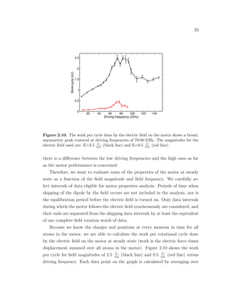
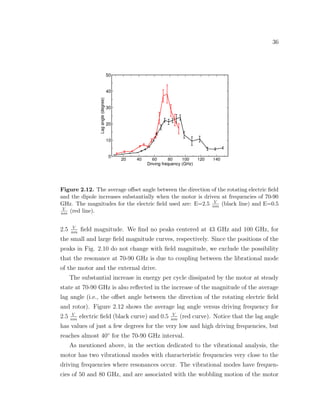
Figure 2.1. Synthetic caltrop-based rotary molecular motor is attached to surfaces
and driven by rotational electric fields. The motor contains a rotor on top, a shaft in
the middle and a three-legged base. The colors of the atoms in the structure are as
follows: carbon-dark blue, hydrogen-green, nitrogen-light blue, oxygen-red, silicon-violet
and sulfur-yellow.
designed to turn the dipole-carrying rotor may also excite other modes within the
system. This gives rise to an increase of friction in the rotary motor system.
Some of the challenges encountered in the rotor systems studied so far are the
decrease of the coupling between the dipole and the underlying surface due to
non-bonded interactions, observed in the case of short rotary motors, and real-
ization of structures that minimize the rotational energy dissipation resulted as a
consequence of resonances with other modes in the system.
Our caltrop-based rotary motor in Fig. 2.1 is another example of a surface-
mounted synthetic molecular machine, engineered to rotate unidirectionally under
the control of rotational electric fields that can be applied between nanofabricated
electrodes situated a couple of micrometers apart. It has been synthesized by J.
Tour at Rice University [37] and is an organic molecule with a size of about 2 nm
in all three spatial directions and a built-in dipole moment in the rotor part of the
molecule. The base of the motor is a molecular structure consisting of four phenyl
rings with tetrahedral spatial orientation which are centered on a silicon atom and
is called a caltrop. A detailed description of the motor is presented in the next
section.

34. 19
Since the rotary motor can function in vacuum and has a small size, we deal
with a system that has a relatively small number of degrees of freedom (some 450
of them), all of which are explicit. This makes the study of dissipation interesting,
because one can follow the loss of energy from the rotational mode of the motor to
all other degrees of freedom explicitly. There are many different external factors
that could affect the performance of the motor, such as field-mediated interactions
or steric interactions with neighboring motors or coupling to the underlying sub-
strate. When studying how our motor dissipates the rotational energy provided
by the external electric field, we focus only on the sources of dissipation arising
from the structure of the motor itself, such as resonances between the external
drive and the soft vibrations within the motor or between the external drive and
the librational mode of the rotor about the instantaneous direction of the external
rotating electric field.
2.2 Static properties of the motor with density
functional theory
In this section, we describe the motor of interest and evaluate some of its static
properties using density functional theory (DFT) calculations.
From a modelling perspective, our caltrop-based rotary molecular motor con-
tains several distinct functional subunits. At top, the dipole-carrying rotor pro-
vides the electrostatic handle by which the motor is driven. The shaft, immediately
below, contains the carbon-carbon triple bond that provides the least-hindered ro-
tational bearing and also introduces additional spatial separation between the rotor
and the underlying surface, in order to reduce possible non-bonded interactions.
The Si atom at the base of the shaft defines the geometric center of the shaft and
the legs of the motor. Further on, the legs provide firm coupling into the substrate
via covalent bonding at their ends. By segmenting the rotary motor into these
subsections, we isolate the most important slow degrees of freedom that govern
the operation of the device, and study their rotational barriers separately. Both
the permanent electrostatic dipole and the induced dipole of the rotor will affect
device operation. The torque applied by an external electric field must drop any

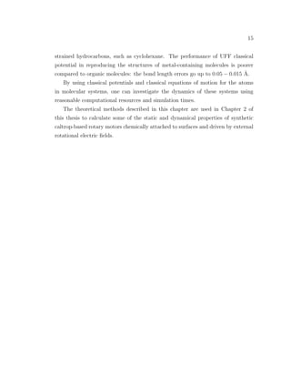
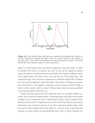
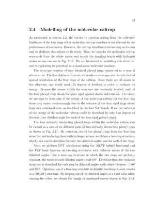
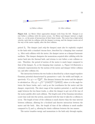
35. 20
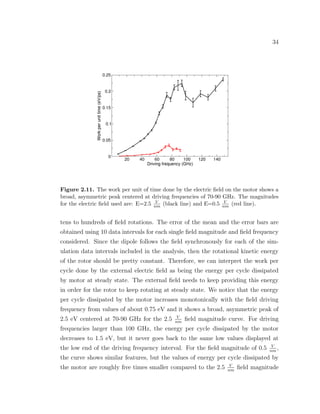
Figure 2.2. Electrostatic potential energy of a 12.5 Debye permanent dipole moment
in an external electric field of 0.5 V
nm as a function of the angle between the field and
the dipole. The red dashed line represents the sinusoidal fit to the electrostatic potential
energy of the dipole in electric field. The black dashed line is the thermal energy at room
temperature.
rotational barrier enough to allow either ballistic motions or thermally induced
asymmetric hopping on a reasonable experimental timescale.
We perform DFT calculations using the B3LYP hybrid functional and the TZV
basis set as implemented in the GAMESS package [38, 39] in order to study the
static properties of the rotary motor. Since electric dipole moments in organic
molecules are essentially local quantities, we separate out the rotor component,
cap the dangling bond with a hydrogen atom, and calculate the charge distribu-
tion. The static electric dipole moment of the rotor is approximately 12.25 Debye,
aligned to within 2.5◦
of the rotor axis as defined by the two nitrogen atoms at its
ends, and can be separated to a good approximation into contributions from the
amine (32%) and NO2 (68%) groups at either end.
The induced moment is much smaller. At an external electric field of 0.5 V
nm
aligned with the static dipole moment (corresponding to ∼500 V across contacts
separated by one micron), the induced moment is about 3 Debye. Since this in-
duced dipole is symmetric under π rotations of the rotor (rather than 2π rotations,

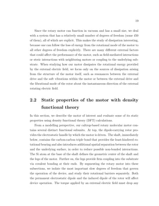
36. 21
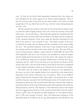
Figure 2.3. Barrier to rotation for the middle bond as a function of the relative angle
between the two benzene rings of the shaft of the motor. The barrier is small and allows
rapid thermally activated rotations about this bond. The black dashed line is the thermal
energy at room temperature.
like the static moment), it does not contribute to the energy difference between
states aligned and anti-aligned to an external electric field. However, it does cause
a small deviation from the sinusoidal dependence of the energy of a rigid static
dipole in an external field, as one can see in Fig. 2.2. The deviation from a curve
corresponding to a rigid dipole, at 90◦
and 270◦
, is due to highly anisotropic po-
larizability for the directions along the rotor and perpendicular to the rotor. The
curve for the electrostatic potential energy of the dipole in the external electric
field of 0.5 V
nm
is symmetric with respect to 180◦
. The rotor can develop a max-
imum torque of about 2.3 meV
deg
or 21 pN · nm. Since the arm of the torque from
the electric field is about 1 nm with respect to the central rotational axis, we ob-
tain that the dipolar unit generates a maximum force of about 20 pN under the
influence of a 0.5 V
nm
electric field. External electric fields of up to 1 - 2 V
nm
can
be achieved experimentally. In comparison, the ATP-synthase biological motor
generates a constant force of 40 pN [2].
The carbon-carbon triple bond within the shaft is the site of least resistance to
rotation, as one can see in Fig. 2.3. It has a barrier of about 46 meV and requires

37. 22
Figure 2.4. The barrier to rotation for the upper bond as a function of the relative
angle between the rotor and the uppermost ring of the shaft of the motor. The strong
interactions between the hydrogen atoms across the bond give rise to a substantial barrier
against rotation. The black dashed line is the thermal energy at room temperature.
an external torque of maximum 0.8 meV
deg
in order to drive rotation, which is about 3
times smaller than the maximum torque provided by an external field of 0.5 V
nm
. In
order to calculate the barrier to rotation, we first remove both the rotor on top and
the base of the motor and satisfy the dangling bonds of the two remaining phenyl
rings with hydrogen atoms. Then, we calculate the energy while rotating the two
rings with respect to each other. The minimum of the barrier corresponds to the
case when the two rings in the shaft are coplanar and the maximum is obtained
when they make a dihedral angle of 90◦
between them. The barrier is small and
allows rapid thermally activated rotations about this bond at room temperature.
Two other sites of possible rotation are also important, not because the system
will actually rotate fully about these points, but because partial rotations within
restricted angle ranges will occur around each of these bonds, and dissipation
upon collision with the extrema of these angular ranges may be significant. Steric
hindrance from opposing hydrogen atoms across these bonds generates large rota-
tional barriers, but substantial angular ranges remain available for partial angular
motions. Figure 2.4 shows the uppermost barrier to rotation, corresponding to the

38. 23
Figure 2.5. The relaxed (black solid line) and unrelaxed (red dashed line) barriers to
rotation obtained by rotating the upper ring of the caltrop structure with respect to
the other three. The barrier is fluctuating and allows intermittent rotation. The black
dashed line is the thermal energy at room temperature.
single C-N bond between the rotor and the uppermost ring of the shaft. In order
to calculate the barrier, we separate the rotor on top and the uppermost phenyl
ring of the shaft in a smaller structure and calculate the energy for different values
of the angle between the plane of the rotor and the one of the phenyl ring. The
minimum energy of the structure corresponds to a dihedral angle of 63.4◦
between
the rotor and the uppermost ring of the shaft. The barrier to rotation is substan-
tial, about 0.83 eV, and requires a maximum external torque of about 27 meV
deg
in
order to drive rotation, which is about 10 times larger than the torque generated
by an external electric field of 0.5 V
nm
.
Finally, the three legs of the base enable the motor to assemble upright on a
surface and to function independently of solvating liquid, providing much weaker
coupling to the environment than would intimate contact with an ambient fluid.
Rotations about the Si–C single bond at the lower end of the shaft are particularly
interesting, since concerted motions of the three uppermost phenyl rings of the
legs and the lowest phenyl ring of the shaft (i.e., the four rings of the molecular
caltrop) can either impose an insurmountable steric wall, or nearly eliminate the

39. 24
rotational barrier about this bond. Figure 2.5 shows the relaxed (black solid line)
and unrelaxed (red dashed line) barriers against rotation for the Si–C single bond
at the lower end of the shaft. In order to calculate the rotational barriers we
separate the molecular caltrop in a smaller structure and satisfy the dangling
bonds with hydrogen atoms. We obtain the unrelaxed barrier against rotation
by rotating the upper ring of the molecular caltrop (i.e., the lowest ring of the
shaft of the motor) with respect to the other three lower rings without allowing
any relaxation of the positions of the latter. This corresponds to a hypothetical
situation when the three lower rings do not actually have any time to move out of
the way when the upper ring rotates. We obtain a substantial barrier to rotation
of about 0.8 eV, which is due to the mutual interactions of the hydrogen atoms
from adjacent rings of the molecular caltrop, when they run into each other. In
order to obtain the relaxed barrier to rotation, we allow the relaxation of the
positions of the three lower rings of the molecular caltrop while rotating the upper
one. This corresponds to a hypothetical situation when the three lower rings move
completely out of the way when the upper ring rotates. In this case, we obtain a
much lower barrier to rotation, of just 0.1 eV. Notice that the relaxed barrier to
rotation has 6 peaks, coming from the 6-fold symmetry of the molecular caltrop
structure (3-fold symmetry due to the presence of the three lower rings and 2-fold
symmetry due to the upper ring). Therefore, the synchronized rotation of the
molecular caltrop rings or the lack of it gives rise to a fluctuating barrier, which
may allow intermittent rotation. However, since the middle bond of the shaft of
the motor allows nearly free rotation, the torque from the external electric field
does not act upon the single Si–C bond at the lower end of the shaft. Thus, this
bond is not important as far as motor device operation is concerned. We present
a more detailed study of the molecular caltrop structure on its own in section 2.4,
below.

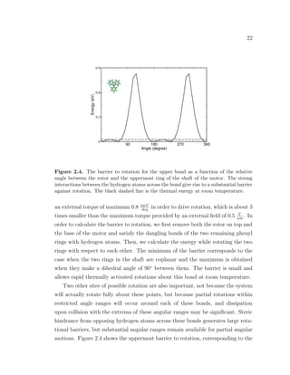
40. 25
2.3 Static and dynamic properties of the motor
with classical molecular dynamics
In this section, we study the dynamical behavior of our caltrop-based molecular
motor and possible mechanisms of energy dissipation that can arise from within
the motor structure. We carry out classical molecular dynamics simulations using
the UFF classical potential, as implemented in the TINK molecular dynamics
package [18].
2.3.1 Assessment of quality of UFF classical potential
First of all, we would like to assess how well UFF classical potential describes some
of the static properties of the motor in comparison to DFT. Therefore, we recal-
culate the barriers to rotation for the upper bond, which makes the connection
between the rotor and the shaft, and for the middle bond within the shaft, where
rotation actually occurs. By isolating the degrees of freedom corresponding to up-
per and middle bonds in smaller structures, we change the side functionality, and,
therefore, the charge distribution within these structures, with respect to the one
in the whole motor structure. In order to determine the effect of structure separa-
tion on the barriers to rotation, for the upper and the middle bonds, respectively,
we calculate the barriers to rotation on several different structures using UFF. We
start with the same small structures used for the DFT calculations (see Fig. 2.3
and 2.4, respectively), and keep enlarging the structures, by adding more phenyl
rings. For each of the upper or middle bonds, respectively, we find no variation of
the barrier to rotation with structure size using UFF. Figures 2.6 and 2.7 below
illustrate the comparison between DFT and UFF classical potential for the upper
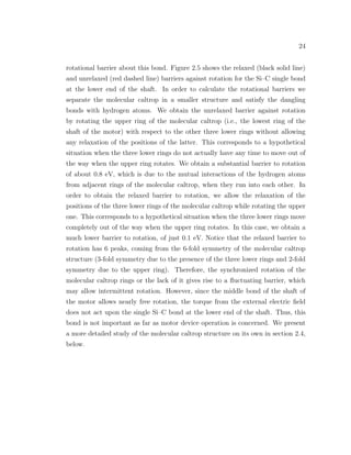
and middle bonds, respectively.
The barrier to rotation due to the upper bond is very similarly described by
both methods. For a relaxed structure, the dihedral angle between the rotor plane
and the upper ring plane is about 40◦
(20◦
smaller compared to a relaxed structure
in DFT). Barrier calculations using a non-resonant atom-type for the nitrogen
atom at the upper bond between rotor and shaft (i.e., using a set of UFF force
field parameters that neglects the contribution of the π orbitals to the barrier),

41. 26
Figure 2.6. Barrier to rotation about the single N–C bond between the rotor and the
upper phenyl ring of the shaft using DFT (black line) and UFF (red line).
Figure 2.7. Barrier to rotation about the triple bond within the shaft of the motor
using DFT (black line) and UFF (red line).
as opposed to a correct resonant atom-type of the UFF classical potential, result
in a barrier with no secondary peaks whatsoever. The main peaks remain as

42. 27
important. This result suggests that, even if expensive DFT barrier calculations
were performed on larger structures, and variations of secondary peaks height with
structure size were obtained, the huge main peaks are independent of the π orbitals
stability. The main peaks are due to the interactions of the hydrogen atoms across
the bond and are almost equal using each method. The character of rotation about
the uppermost bond of the motor is determined by the substantial main peaks,
not the small secondary ones. The small offset between the tips of the main peaks
is just an artifact of the method by which the UFF barrier is calculated. The
secondary peaks in Fig. 2.6, due to the breaking of the π orbital alignment, are
overestimated in UFF compared to DFT. This results in an additional restriction of
the angular intervals available for partial rotations about this bond, which might
overestimate the coupling between the rotational motion of the rotor and high
vibrational modes in the motor.
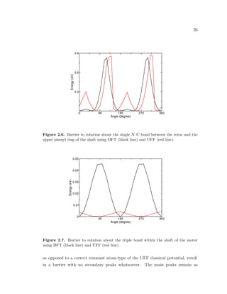
The middle bond barrier to rotation (see Fig. 2.7) is some 10 times under-
estimated in UFF compared to DFT. Also, notice that the peaks of the barrier
in UFF are shifted 90◦
compared to DFT. Optimization in UFF gives a dihedral
angle of 90◦
between the planes of the two shaft rings for the relaxed structure
of the shaft, while DFT optimizes the shaft with the two rings perfectly aligned.
Other studies for the barrier to rotation, using quantum mechanics calculations, in
a variety of systems containing carbon-carbon triple bonds, and in the absence of
steric hindrance, report extremely close values to the one we found using DFT (see
review article on rotary motors [36]). Although there is a big discrepancy between
the DFT and the UFF description for the barrier to rotation of the middle bond,
the barrier in both cases is very low and comparable to thermal energy, allowing
rapid spontaneous rotation at ambient temperatures. For example, one possible
consequence of this barrier underestimation by UFF classical potential is that the
molecular dynamics simulations might overestimate the upper limit of the field
frequency at which the motor is able to follow the electric field. However, this
effect would become important for weak electric fields and very low temperatures,
when rotation is determined by thermal hopping over the rotational barrier.
The permanent dipole moment of the motor is calculated to be about 15.8 De-
bye using the UFF classical potential and is localized only on the rotor, just as in
DFT. Although it is almost 30% larger compared to the permanent dipole moment

43. 28
of the rotor given by DFT with no external field applied, this value is actually very
close to the one given by DFT for a dipole in an external electric field of about
0.5 V
nm
along the dipole direction. Also, the TINK molecular dynamics package
does not take into consideration any contribution to the dipole due to the pres-
ence of external electric fields. The discrepancy between the values of the dipole
moments as calculated by the two theoretical methods results in overestimation of
the driving force that the electric field applies to the dipole, which further leads
to overestimation of the motor performance at high driving frequencies.
By decomposing the total dipole moment of the rotor (consisting of 50 atoms)
into components parallel and perpendicular to the vertical motor shaft (as defined
by the vector between the Si atom at the base and the middle N atom of the
rotor) we determine that the dipole is oriented 17◦
with respect to the direction
perpendicular to the shaft. We also calculate the relative orientation between
the vertical shaft of the motor and the rotor (as defined by the vector between
the two nitrogen atoms situated at the ends of the rotor) for an optimized motor
structure using UFF classical potential and we find an angle of about 2◦
(NO end
of rotor is lower). Therefore, from a purely geometrical point of view, the rotor
itself is not precisely perpendicular to the shaft. A similar purely geometrical
analysis reveals an angle of about 6◦
between the shaft and the rotor for a motor
structure optimized using an ab-initio level of approximation. We do not know
the direction of the dipole nor the one of the dipole-carrying rotor with respect to
the direction of the shaft in DFT because such a calculation is computationally
expensive. However, since the external rotational electric field lies in the horizontal
plane, it is conceivable that the dipole can induce additional oscillations into the
system, in its attempt to align with the horizontal direction.
2.3.2 Vibrational analysis
We perform vibrational mode frequency calculations on the motor structure in
an attempt to find which soft modes of the motor are likely to couple to the
external electric field and give rise to increased dissipation. We carry out the
vibrational analysis within the approximation of the UFF classical potential using
the partial Hessian vibrational analysis (PHVA) [40] as implemented in the TINK

44. 29
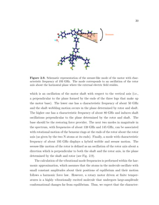
Figure 2.8. Schematic representation of the wobbling modes of the motor with char-
acteristic frequencies of 50 and 80 GHz. The mode corresponds to an oscillation of the
motor shaft with respect to the vertical axis.
molecular dynamic package. The method is extensively used for partially optimized
systems, for example, adsorbates on surfaces [41]. We first perform a constrained
optimization of the motor structure, in which two end atoms from each of the
three legs of the motor are constrained to fixed positions (same atoms are fixed for
all of the MD calculations performed on this motor). Then, we continue with the
partial vibrational mode frequency calculation. The PHVA method diagonalizes
only a subblock of the Hessian matrix to yield vibrational frequencies, the one
corresponding to the non-fixed atoms. We keep those few leg atoms fixed in order
to simulate the attachment of the motor to a surface.
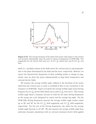
We find that the vibrational spectrum of the motor covers values from 13 GHz
up to a little over 100 THz. Since we drive the motor at frequencies close to the
softer modes of the motor rather than the stiffer ones, and since only the lowest
15% of the vibrational modes are excited at room temperature, we do not consider
the higher end of the vibrational spectrum further. A few soft modes of the motor
have magnitudes within the driving frequency interval for the external electric field
(10-150 GHz) and we present them here in more detail. Two of the modes of the
motor are associated with what we call the shaft wobbling motion (see Fig. 2.8),

45. 30
Figure 2.9. Schematic representation of the seesaw-like mode of the motor with char-
acteristic frequency of 193 GHz. The mode corresponds to an oscillation of the rotor
axis about the horizontal plane where the external electric field resides.
which is an oscillation of the motor shaft with respect to the vertical axis (i.e.,
a perpendicular to the plane formed by the ends of the three legs that make up
the motor base). The lower one has a characteristic frequency of about 50 GHz
and the shaft wobbling motion occurs in the plane determined by rotor and shaft.
The higher one has a characteristic frequency of about 80 GHz and induces shaft
oscillations perpendicular to the plane determined by the rotor and shaft. The
base should be the restoring force provider. The next two modes in magnitude in
the spectrum, with frequencies of about 138 GHz and 145 GHz, can be associated
with rotational motion of the benzene rings at the ends of the rotor about the rotor
axis (as given by the two N atoms at its ends). Finally, a mode with characteristic
frequency of about 193 GHz displays a hybrid wobble and seesaw motion. The
seesaw-like motion of the rotor is defined as an oscillation of the rotor axis about a
direction which is perpendicular to both the shaft and the rotor axis, in the plane
determined by the shaft and rotor (see Fig. 2.9).
The calculation of the vibrational mode frequencies is performed within the har-
monic approximation, which assumes that the atoms in the molecule oscillate with
small constant amplitudes about their positions of equlibrium and their motion
follows a harmonic force law. However, a rotary motor driven at finite temper-
atures is a highly vibrationally excited molecule that undergoes large-amplitude
conformational changes far from equilibrium. Thus, we expect that the character-

46. 31
istic frequencies of the modes discussed above to change in value when the motor is
driven anharmonically at room temperature and energy flows between the different
modes of the motor.
2.3.3 Dynamic behavior in external electric field
In order to investigate the performance of the motor under external drive and to
elucidate the role of possible resonances, we perform classical molecular dynamics
simulations on the motor.
We drive the motor using electric field magnitudes of 0.5 V
nm
and 2.5 V
nm
, and
electric field frequencies between 10 and 150 GHz. The thermal rotation of the
rotor at temperatures comparable to room temperature is about 25 GHz, close
to the low end of the driving frequency interval. The frequency of the thermal
rotation of the rotor is calculated according to the equipartition theorem, which
states that in thermal equilibrium, energy is shared equally among all degrees of
freedom of the system. Given the large values for the magnitudes of the electric
fields that we use and the big dipole moment of the rotor, we operate in a regime
where the driving force is the dominant factor that determines the performance of
the motor. Other forces within the system that could influence the performance of
the motor, such as the thermal fluctuations and the rotational barrier about which
rotation occurs, are much weaker compared to the external drive. The lengths of
the simulations vary from several tens of field rotations for the small magnitude
driving frequencies and up to a few hundred field rotations for the large magnitude
driving frequencies (i.e., between 1 ns and 4 ns total simulation time per run).
We thermalize all degrees of freedom with no external field applied at 250 K
for 80 ps (i.e., 80,000 steps equilibration period). Then, we adjust the electric
field angle to align with the rotor at that moment in time and impose the rotating
external field. Beyond the equilibration period, we consider two different methods
in order to control the temperature of the motor during the simulation. In the
first method, called the non-thermostatted system method, the thermostat is en-
tirely decoupled from the motor at the end of the 80 ps equlibration period when
the field is turned on. In the second method, called the partially thermostatted
system method, the thermostat at 250 K remains coupled only to the base of the

47. 32
motor at the end of the 80 ps period when the field is turned on. The role of
a thermostat is to keep a system in thermal equilibrium at a specific tempera-
ture. Since the rotor of the motor engages in large-amplitude, ordered motion
far from thermal equilibrium, we avoid its direct coupling to a thermostat. For
the non-thermostatted case, the motor heats up substantially over the course of
the simulation because the external field does work on it, adding energy into the
system. The temperature of the motor reaches several hundred Kelvin (for the
small field magnitudes and frequencies) or even a few thousand Kelvin (for the
large field magnitudes and frequencies). Since some of the physical properties of
the system may be severely altered due to indirect effects arising from the gradual
heating up of the motor during the run, we also want to couple a thermostat just
to the device non-relevant degrees of freedom (i.e., those at the base). The partial
thermostatting of the system is meant to keep a constant temperature during the
run. In a real experiment, the substrate would serve as thermostat for the motor,
preventing it from heating up. A thermostat attached to the legs or the legs plus
the shaft seems to control the temperature quite nicely, with a slightly elevated
temperature in the rotor compared to the thermostatted base. We notice also that
the shaft engages in organized non-thermal motions to some extent, not only the
driven rotor. Therefore, we decide to perform our molecular dynamics analysis
with only the base of the motor coupled to a thermostat. A legs-only thermostat
keeps the shaft of the motor and rotor temperature down to reasonable values, up
to 100 K heating relative to the base for the large magnitude fields and driving
frequencies.
For the 2.5 V
nm
electric field magnitude, the motor follows the field without
skipping any of the field rotations (i.e., synchronous motion) up to 50 GHz. For
larger driving frequencies, the motor skips on average less than 7% of the field
rotations, for each driving frequency. For the smaller field magnitude, E=0.5 V
nm
,
the motor has an asynchronous motion for the whole range of driving frequencies.
On average, the motor skips about 7% of the total number of field rotations for
field frequencies under 50 GHz. For driving frequencies above 50 GHz, the number
of times the motor skips the field increases monotonically between 20% and 60%
of the total number of field rotations. The motor becomes unable to follow the
field at driving frequencies above 90 GHz for this field magnitude. It appears that

48. 33
Figure 2.10. The work per cycle done by the electric field on the motor shows a broad,
asymmetric peak centered at driving frequencies of 70-90 GHz. The magnitudes for the
electric field used are: E=2.5 V
nm (black line) and E=0.5 V
nm (red line).
there is a difference between the low driving frequencies and the high ones as far
as the motor performance is concerned.
Therefore, we want to evaluate some of the properties of the motor at steady
state as a function of the field magnitude and field frequency. We carefully se-
lect intervals of data eligible for motor properties analysis. Periods of time when
skipping of the dipole by the field occurs are not included in the analysis, nor is
the equilibration period before the electric field is turned on. Only data intervals
during which the motor follows the electric field synchronously are considered, and
their ends are separated from the skipping data intervals by at least the equivalent
of one complete field rotation worth of data.
Because we know the charges and positions at every moment in time for all
atoms in the motor, we are able to calculate the work per rotational cycle done
by the electric field on the motor at steady state (work is the electric force times
displacement summed over all atoms in the motor). Figure 2.10 shows the work
per cycle for field magnitudes of 2.5 V
nm
(black line) and 0.5 V
nm
(red line) versus
driving frequency. Each data point on the graph is calculated by averaging over

49. 34
Figure 2.11. The work per unit of time done by the electric field on the motor shows a
broad, asymmetric peak centered at driving frequencies of 70-90 GHz. The magnitudes
for the electric field used are: E=2.5 V
nm (black line) and E=0.5 V
nm (red line).
tens to hundreds of field rotations. The error of the mean and the error bars are
obtained using 10 data intervals for each single field magnitude and field frequency
considered. Since the dipole follows the field synchronously for each of the sim-
ulation data intervals included in the analysis, then the rotational kinetic energy
of the rotor should be pretty constant. Therefore, we can interpret the work per
cycle done by the external electric field as being the energy per cycle dissipated
by motor at steady state. The external field needs to keep providing this energy
in order for the rotor to keep rotating at steady state. We notice that the energy
per cycle dissipated by the motor increases monotonically with the field driving
frequency from values of about 0.75 eV and it shows a broad, asymmetric peak of
2.5 eV centered at 70-90 GHz for the 2.5 V
nm
field magnitude curve. For driving
frequencies larger than 100 GHz, the energy per cycle dissipated by the motor
decreases to 1.5 eV, but it never goes back to the same low values displayed at
the low end of the driving frequency interval. For the field magnitude of 0.5 V
nm
,
the curve shows similar features, but the values of energy per cycle dissipated by
the motor are roughly five times smaller compared to the 2.5 V
nm
field magnitude

50. 35
case. At least for the electric field magnitudes considered here, the energy per
cycle dissipated by the motor appears to be linear in field magnitude. Also, we
plot the work per unit of time done by the electric field on the motor, for field
magnitudes of 2.5 V
nm
(black line) and 0.5 V
nm
(red line) versus driving frequency
(see Fig. 2.11).
We also calculate the work per cycle done by the external electric field in order
to rotate the built-in dipole moment of the rotor about the direction of the shaft
of the motor. Let us call it Wdipole. We obtain this quantity by evaluating both the
component of the external torque from the field on the dipole and the component
of the rotational frequency of the rotor along the direction determined by the
shaft of the motor at every moment in time. The dipole moment of the rotor
is calculated by using only the charges and the coordinates of the atoms within
the rotor. The rotational frequency of the rotor is also calculated based on only
the positions and the velocities of the atoms within the rotor. The plot of Wdipole
versus driving frequency displays a peak centered at 70-90 GHz for both of the
field magnitudes used, just as the work per cycle calculated by using the charges
and the displacements for all atoms in the entire motor. We compare the work per
cycle calculated by using the two methods outlined above, and find that Wdipole
represents only 30 − 60% of the total work per cycle done by the field on all the
atoms of the motor. The rest of the work per cycle done by the motor is dissipated
in other degrees of freedom, which are not relevant for the rotation of the dipole.
We believe that the peaks in the graphs for energy per cycle dissipated by
the motor are due to the coupling between the external drive and characteristic
frequencies of the system, which gives rise to resonances. There are two different
types of characteristic frequencies that could couple to the external drive: a char-
acteristic frequency associated with the librational motion of the dipole about the
instantaneous direction of the external electric field and a characteristic frequency
associated with one of the motor vibrational modes with magnitude well within the
driving frequency interval. The frequency of the librational motion of the dipole
about the instantaneous direction of the external electric field is directly propor-
tional to PE
I
, where E represents the field magnitude, P is the dipole moment,
and I is the rotor moment of inertia. Here, the characteristic frequency of the
librational mode is 43 GHz for the 0.5 V
nm
field magnitude and 100 GHz for the

51. 36
Figure 2.12. The average offset angle between the direction of the rotating electric field
and the dipole increases substantially when the motor is driven at frequencies of 70-90
GHz. The magnitudes for the electric field used are: E=2.5 V
nm (black line) and E=0.5
V
nm (red line).
2.5 V
nm
field magnitude. We find no peaks centered at 43 GHz and 100 GHz, for
the small and large field magnitude curves, respectively. Since the positions of the
peaks in Fig. 2.10 do not change with field magnitude, we exclude the possibility
that the resonance at 70-90 GHz is due to coupling between the librational mode
of the motor and the external drive.
The substantial increase in energy per cycle dissipated by the motor at steady
state at 70-90 GHz is also reflected in the increase of the magnitude of the average
lag angle (i.e., the offset angle between the direction of the rotating electric field
and rotor). Figure 2.12 shows the average lag angle versus driving frequency for
2.5 V
nm
electric field (black curve) and 0.5 V
nm
(red curve). Notice that the lag angle
has values of just a few degrees for the very low and high driving frequencies, but
reaches almost 40◦
for the 70-90 GHz interval.
As mentioned above, in the section dedicated to the vibrational analysis, the
motor has two vibrational modes with characteristic frequencies very close to the
driving frequencies where resonances occur. The vibrational modes have frequen-
cies of 50 and 80 GHz, and are associated with the wobbling motion of the motor

52. 37
Figure 2.13. The average deviation of the shaft of the motor with respect to the vertical
axis increases substantially when the motor is driven at frequencies of 70-90 GHz. The
magnitudes for the electric field used are: E=2.5 V
nm (black line) and E=0.5 V
nm (red
line).
shaft (i.e., pendular motion of the shaft about the vertical axis) in and perpendic-
ular to the plane determined by the shaft and the rotor, respectively. However, we
expect the characteristic frequencies of these wobbling modes to change in mag-
nitude, since we drive the motor anharmonically at large finite temperature and
external electric fields.
We measure the average wobble angle, defined as the deviation of the motor
shaft from the vertical axis, in order to establish if there is any correlation to the
resonance at 70-90 GHz. Figure 2.13 shows the average wobble angle versus driving
frequency for 2.5 V
nm
electric field (black curve) and 0.5 V
nm
(red curve). The average
wobble angle shows a dramatic increase in value for the same driving frequencies
as the energy per cycle dissipated by motor and the average lag angle. For the
70-90 GHz driving frequencies interval, the average wobble angle reaches values
up to 30◦
and 50◦
for the 0.5 V
nm
field magnitude and 2.5 V
nm
field magnitude,
respectively. For the rest of the driving frequencies, the values for the average
wobble angle decrease to 18◦
-20◦
. We also measure the average wobble angle from
molecular dynamics simulations with no external rotational electric field applied

53. 38
(a) (b)
Figure 2.14. Movie snapshots illustrating the dynamical behavior of the motor when
driven at (a) 75 GHz, and (b) 150 GHz, respectively. Field magnitude equals 2.5 V
nm. At
resonance, the shaft of the motor undergoes large amplitude motions, causing the rotor
to sweep the substrate underneath.
and we find a value of 18◦
. Therefore, the shaft wobbling outside of the resonance
driving frequency interval is due to the softness of the motor wobbling mode.
Figures 2.14 (a) and (b) illustrate movie snapshots corresponding to dynamical
behavior of the motor when driven at 75 GHz and 150 GHz, respectively, and
2.5 V
nm
field magnitude. When driven at frequencies close to the resonance interval
(see Fig. 2.14(a)), the shaft of the motor displays large amplitude motions, causing
the rotor to virtually sweep the substrate underneath. For other driving frequencies
(see Fig. 2.14(b)), the shaft undergoes smaller amplitude motions and maintains
the position of the rotor in the horizontal plane, where the electric filed resides.
Therefore, the results shown in Fig. 2.13, in combination with the movies, lead
to the conclusion that the resonance at 70-90 GHz is due to coupling between the
rotational external drive and the wobbling modes of the motor with characteristic
frequencies in the vecinity of that frequency interval.
The elastic deviation of the shaft from the vertical axis results in a misalign-
ment of the dipole-carrying rotor with respect to the horizontal plane where the

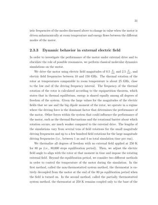
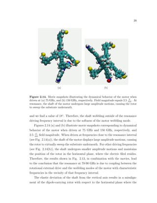
54. 39
rotational electric field resides. The softness of the shaft is the major design issue
of our rotary motor since it leads to increased dissipation and poor performance
when driven at frequencies close to those of the soft modes of the motor. Another
simulation-based study reported a similar competition between the induction of
rotational motion of the rotor and the excitement of pendulum-like motion of the
shaft for a rotary motor [18]. Therefore, there is a need for designing rotary motors
with more rigid shafts in order to constrain the motion of the rotor to the plane
where the external electric field resides.
2.3.4 Field-free decay analysis
In this section, we examine the field-free decay of the rotational motion. After a
80 ps period of thermal equilibration, we assign additional velocity vectors corre-
sponding to rotational excitations in the range of 10 to 150 GHz to all atoms of
the rotor and we monitor the subsequent motion of the motor. We notice that
the component of the rotor angular momentum along the direction defined by the
shaft of the motor, L(t), decays from its initial value, L(0), rapidly at the begin-
ning and then increasingly slowly. The rotational excitation of the rotor ceases to
be detectable after a maximum of 100 ps. In this time, the rotor transitions from
unidirectional rotation to random rotation.
According to the Langevin Eqn. (2.1) introduced above, a rotor directly cou-
pled to a thermal bath, under the direct influence of a viscous force proportional
to its own speed and that of thermal forces, loses energy and momentum following
an exponential law in time. That is: L(t) = L(0)e− t
τ , where τ represents the decay
time constant or relaxation time. Assuming exponential decay for the component
of the angular momentum of the rotor about the direction defined by the shaft of
the motor, we plot log (L(t)
L(0)
) versus time and fit the data with a straight time in
the attempt to extract a decay time constant for the motor.
We are unable to extract a decay time constant for rotational excitations of the
rotor corresponding to frequencies comparable to the thermal rotation frequency
at room temperature, i.e., 25 GHz. For rotational excitations corresponding to
higher frequencies, the data fit a straight line. We use the inverses of the slopes of
these fits to obtain an average decay time constant for the motor.

55. 40
(a)
(b)
Figure 2.15. Plots of log ( L(t)
L(0)) versus time (black) and the corresponding linear fits
(red line) for two different initial rotational excitations: (a) 30 GHz (τ=47.5 ps) and (b)
150 GHz (τ=41 ps).

56. 41
Figure 2.16. The molecular caltrop consists of four identical phenyl rings connected to
a central silicon atom. The structure might function as a molecular gear if the rotary
power generated by mechanically driving one ring would get transmitted to the other
rings via concerted rotations.
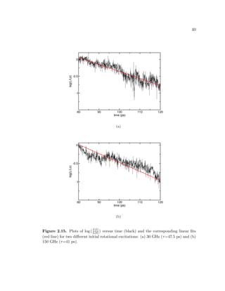
Figure 2.15 shows the plots of log (L(t)
L(0)
) versus time (black) and the correspond-
ing linear fits (red line) for two different initial rotational excitations: (a) 30 GHz
(τ=47.5 ps) and (b) 150 GHz (τ=41 ps).
We are not able to detect any significant differencies between the values for
the decay time constants obtained as a function of the frequency. Therefore, we
average over all the runs and obtain a decay time constant of circa 38 ps. In
comparison, different molecular dynamics studies of field-driven surface-attached
rotary motors reported average decay time constants of 83 ps [32] and just a few
picoseconds [33].
The motor thermalizes rotational excitations corresponding to energies of sev-
eral tenths of electron volts in excess of the thermal energy in just several tens of
picoseconds, or the equivalent of up to 10 complete rotations of the rotor. This fast
relaxation is due to a combination between the effect of the thermal fluctuations
within the motor and the coupling between the torsional mode that alows rotation
and the other vibrational modes of the motor.

57. 42
2.4 Modelling of the molecular caltrop
As mentioned in section 2.2, the barrier to rotation arising from the collective
hindrance of the four rings of the molecular caltrop structure is not relevant to the
performance of our motor. However, the caltrop structure is interesting on its own
and we dedicate this section to its study. Thus, we consider the molecular caltrop
separately from the whole motor and satisfy the dangling bonds with hydrogen
atoms as one can see in Fig. 2.16. We are interested in modelling this structure
and in exploiting its potential as a stand-alone molecular machine.
The structure consists of four identical phenyl rings connected to a central
silicon atom. The four-fold coordination of the silicon atom governs the tetrahedral
spatial orientation of the four rings of the caltrop. Since there are 45 atoms in
the structure, one would need 135 degrees of freedom in order to evaluate its
energy. Because the atoms within the structure are covalently bonded, each of
the four phenyl rings should be quite rigid against elastic deformation. Therefore,
we attempt to determine if the energy of the molecular caltrop (or the four-ring
structure) varies predominantly due to the rotation of the four rigid rings about
their own rotational axes, as described by the four Si-C bonds. If so, the variation
of the energy of the molecular caltrop could be described by only four degrees of
freedom (one dihedral angle for each of the four rigid phenyl rings).
The four mutually interacting phenyl rings within the molecular caltrop can
be viewed as a sum of six different pairs of two mutually interacting phenyl rings
as shown in Fig. 2.17. By removing two of the phenyl rings from the four-ring
structure and replacing them with hydrogen atoms, we obtain a two-ring structure,
which then can be described by only two dihedral angles, one for each of the rings.
Next, we perform DFT calculations using the B3LYP hybrid functional and
the TZV basis function on two-ring structures with different values of the two
dihedral angles. For a two-ring structure in which the two rings are perfectly
coplanar, the values of each dihedral angle is called 0◦
. Deviation from the coplanar
structure is described for each ring by dihedral angles with values between −180◦
and 180◦
. Optimization of a two-ring structure in density functional theory results
in a (90◦
,90◦
) structure. By keeping one of the dihedral angles at a fixed value while
varying the other, we obtain the family of unrelaxed curves shown in Fig. 2.18.

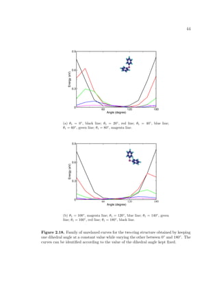
58. 43
Figure 2.17. The four mutually interacting phenyl rings within the molecular caltrop
can be viewed as a sum of six different pairs of two mutually interacting phenyl rings.
For each of these curves, the energy of the two-ring structure is calculated by
allowing only electron relaxation, the nuclei do not relax (i.e., called single point
energy calculations). We find that the highest energy configurations of the two-
ring structure correspond to small values of the two dihedral angles, when the
interactions between the hydrogen atoms coming from the two rings are strong.
The family of relaxed curves, obtained by allowing positional relaxation for both
the electrons and the nuclei (i.e., called optimization calculations), while keeping
the two dihedral angles of the two-ring structure at fixed values, are not shown.
We fit the DFT data for the unrelaxed and/or the relaxed two-ring structures
to a basis set of sine and cosine functions in order to obtain an analytical function
to describe the energy of the two-ring structure as a function of the dihedral angles.
We find that each of the curves in Fig. 2.18 can be fitted well with the following
function:
n
i=0
(A1 sin [iθ1] + B1 cos [iθ1]), with n a positive even integer and A1, B1
real numbers. Since the two phenyl rings and their spatial orientations are iden-
tical, we propose an energy function for the two-ring structure that is symmetric
with respect to the two dihedral angles:
g(θ1, θ2) =
n
i=0
(A1 sin [iθ1] + B1 cos [iθ1])
n
j=0
(A2 sin [jθ2] + B2 cos [jθ2]) ,(2.2)
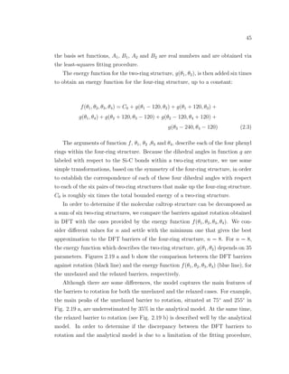
with i, j and n positive integers and even numbers. The coefficients in front of

59. 44
(a) θ1 = 0◦
, black line; θ1 = 20◦
, red line; θ1 = 40◦
, blue line;
θ1 = 60◦
, green line; θ1 = 80◦
, magenta line.
(b) θ1 = 100◦
, magenta line; θ1 = 120◦
, blue line; θ1 = 140◦
, green
line; θ1 = 160◦
, red line; θ1 = 180◦
, black line.
Figure 2.18. Family of unrelaxed curves for the two-ring structure obtained by keeping
one dihedral angle at a constant value while varying the other between 0◦ and 180◦. The
curves can be identified according to the value of the dihedral angle kept fixed.

60. 45
the basis set functions, A1, B1, A2 and B2 are real numbers and are obtained via
the least-squares fitting procedure.
The energy function for the two-ring structure, g(θ1, θ2), is then added six times
to obtain an energy function for the four-ring structure, up to a constant:
f(θ1, θ2, θ3, θ4) = C0 + g(θ1 − 120, θ2) + g(θ1 + 120, θ3) +
g(θ1, θ4) + g(θ2 + 120, θ3 − 120) + g(θ2 − 120, θ4 + 120) +
g(θ3 − 240, θ4 − 120) (2.3)
The arguments of function f, θ1, θ2 ,θ3 and θ4, describe each of the four phenyl
rings within the four-ring structure. Because the dihedral angles in function g are
labeled with respect to the Si-C bonds within a two-ring structure, we use some
simple transformations, based on the symmetry of the four-ring structure, in order
to establish the correspondence of each of these four dihedral angles with respect
to each of the six pairs of two-ring structures that make up the four-ring structure.
C0 is roughly six times the total bounded energy of a two-ring structure.
In order to determine if the molecular caltrop structure can be decomposed as
a sum of six two-ring structures, we compare the barriers against rotation obtained
in DFT with the ones provided by the energy function f(θ1, θ2, θ3, θ4). We con-
sider different values for n and settle with the minimum one that gives the best
approximation to the DFT barriers of the four-ring structure, n = 8. For n = 8,
the energy function which describes the two-ring structure, g(θ1, θ2) depends on 35
parameters. Figures 2.19 a and b show the comparison between the DFT barriers
against rotation (black line) and the energy function f(θ1, θ2, θ3, θ4) (blue line), for
the unrelaxed and the relaxed barriers, respectively.
Although there are some differences, the model captures the main features of
the barriers to rotation for both the unrelaxed and the relaxed cases. For example,
the main peaks of the unrelaxed barrier to rotation, situated at 75◦
and 255◦
in
Fig. 2.19 a, are underestimated by 35% in the analytical model. At the same time,
the relaxed barrier to rotation (see Fig. 2.19 b) is described well by the analytical
model. In order to determine if the discrepancy between the DFT barriers to
rotation and the analytical model is due to a limitation of the fitting procedure,

61. 46
(a)
(b)
Figure 2.19. Comparison between the DFT data (black lines) and the analytical model
(blue lines) for the unrelaxed (a) and the relaxed (b) barriers against rotation of the
four-ring structure.
we try both the case when all DFT data points are weighted equally and the case
when the data points associated to the peaks of the unrelaxed barrier to rotation

62. 47
are weighted 100 times less than the rest. Neither of these cases improves the
fit. We believe that the discrepancy between the DFT barriers to rotation for the
four-ring structure and the analytical model is not due to faulty fitting procedures,
but is intrinsic to a distinction between the four-ring structure and the two-ring
structure that we outline below.
For an optimized two-ring structure, the C-Si-C angle between the two phenyl
rings is about 114◦
. For an optimized and unconstrained four-ring structure, the
values of the six C-Si-C angles describing each pair of rings within the four-ring
structure are on average 110◦
. They can vary anywhere between 107◦
and 112◦
when we apply constraints to keep some of the dihedral angles within the four-ring
structure at specific values, but mostly their values lie in the middle of that interval.
Therefore, a two-ring pair within a two-ring structure is different from one with
the same values of the dihedral angles within the four-ring structure. Because the
value of the C-Si-C angle is larger in a two-ring structure compared to a four-ring
structure, also the distances between hydrogen atoms which belong to adjacent
phenyl rings are always larger in a two-ring structure. Since the main peaks and
also the secondary hunchbacks in Fig. 2.19 are due to strong interactions between
hydrogen atoms situated on adjacent phenyl rings, we believe that the intrinsic
distinction between the two-ring structure and the four-ring structure leads to
their underestimation by the analytical model.
Despite the differences between the DFT barriers to rotation for the four-ring
structure and the analytical model that we presented above, we conclude that the
molecular caltrop in Fig. 2.16 can indeed be decomposed as a sum of six two-
ring structures and can be characterized energetically using only four degrees of
freedom (i.e., a set of four dihedral angles describing each of the four rings of the
structure) instead of 135.
Finally, we attempt to evaluate the potential of the molecular caltrop to func-
tion as a molecular machine on its own. One possibility would be to induce directed
motion into the upper ring mechanically, or to functionalize it with built-in dipole
moments and use electric fields to drive it. The upper ring would play the role of
the rotor and the lower three rings that of the stator. The rate of rotation of the
rotor could vary anywhere between less than 1 Hz and up to hundreds of GHz as
a consequence of the synchronized rotation of the caltrop rings or the lack of it.

63. 48
Figure 2.20. Variation of the dihedral angles corresponding to the three lower phenyl
rings of the molecular caltrop (red, green and blue lines) while the upper phenyl ring
(black line) rotates every 10◦ for a total of 180◦.
If the directed rotary motion induced in one of the rings using some sort of
input energy (mechanical, electrical, chemical, etc.) were transmitted to the other
rings via concerted rotations, the molecular caltrop could serve as a molecular
gear. The goal would be to use the molecular gear to change the spatial direction
along which the rotary motion propagates. Besides allowing concerted rotations
between adjacent rings, the molecular gear would need to have an energetically
costly gear slippage (i.e., very high energies would be necessary to rotate one of
the rings, while keeping the others fixed).
In order to search for proof of correlated motions between the four phenyl
rings of the molecular caltrop, we monitor the variation of the dihedral angles
associated with the three lower rings while the upper ring is rotated every 10◦
for
a total of 180◦
. Figure 2.20 shows the values of the four dihedral angles versus the
indices of the intermediate caltrop structures used to obtain the relaxed barrier
against rotation about the single Si–C bond in Fig. 2.5. The values of the dihedral
angles are obtained by rotating the upper ring with respect to the lower three and
creating 18 initial structures, which are then relaxed, while keeping the value of

64. 49
the dihedral angle for the upper ring fixed. Also, the unrelaxed barrier against
rotation in Fig. 2.5 serves as the gear slippage curve.
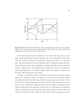
Figure 2.20 shows clear evidence that the rotation of the upper ring causes the
lower rings to rotate partially with respect to their own rotational axes, but it does
not provide enough information for the range of induced partial rotations or if total
concerted rotations are possible. Additional evaluations of the four dihedral angles
would be necessary on a series of caltrop structures where the next structure in the
series is obtained by alternately rotating the upper ring and relaxing the structure
at the specified angle, and so on. Also, molecular dynamics calculations would
test the performance of the gear at finite temperatures. A comprehensive review
of molecular gears is presented by Kottas et al. [36].
2.5 Conclusions
Our theoretical calculations and simulations using DFT and UFF classical poten-
tial prove that external rotating electric fields with magnitudes accessible experi-
mentally induce unidirectional and repetitive rotation of the dipole-carrying rotor
of the motor. The rotation occurs about the triple bond within the shaft of the
motor. Resonances between the external drive and the soft modes associated with
the deviation of the shaft of the motor with respect to the vertical axis give rise
to a dramatic increase in friction within the motor. This further leads to a lack
of control over the dipole-carrying rotor, designed to move in the horizontal plane
where the external electric field resides.
The molecular caltrop, which makes up the basis of our synthetic rotary motor,
can be described using only four degrees of freedom and may have potential to
function as a molecular machine on its own.
Theoretical investigations can provide guidance to help design motor structures
that allow a higher degree of external control, such that the induced motion is
constrained to a very small number of degrees of freedom.

65. Chapter 3
Power law dissipation in motors
indirectly coupled to a thermal bath
3.1 Introduction
In this section, we present a novel mechanism of dissipation in nanoscale and
molecular-scale motors. We describe a regime in which the deceleration of an
unpowered motor follows a universal power law, rather than a standard exponential
decay.
In larger systems and in traditional treatments of small systems, the motor is
directly and continuously coupled to a large number of degrees of freedom, coming
from the motor’s stator or the environment, which are integrated out into a thermal
bath. The motor is coupled directly to this bath via phenomenological terms such
as viscous damping or Langevin forces [32, 33, 36]. If, for example, the viscous
damping force that acts on the motor is proportional to the speed of the motor,
then the motor dissipates energy and momentum in time following an exponential
law [32,33]. Also, the system has an intrinsic time scale.
As the size of the motors decreases and the design of their structures becomes
highly controllable, it becomes feasible to restrict the coupling between the motor
and the thermal bath to just a very small number of degrees of freedom and to
introduce dissipation in a controlled way.
We study a novel situation where one degree of freedom is pulled out from

66. 51
the thermal bath and given an explicit equation of motion. The motor becomes
indirectly coupled to the thermal bath, via only one degree of freedom, which is
interposed between itself and the bath. The motor loses energy and momentum
only through periodic, elastic collisions with this special degree of freedom, which
we call the damper. The damper is directly coupled to the thermal bath. The pur-
pose of our work is to investigate how the motor dissipates energy and momentum
in time in the novel situation of an indirect, discrete and well-defined coupling to
the thermal bath.
We consider periodic, elastic head-on collisions between a large, heavy motor
of mass M and a small, light damper of mass m. The motor starts out with some
initial momentum and the damper is at rest before each collision. The collisions
between the masses occur instantaneously. By using conservation of energy and
momentum for the elastic collisions between the motor and the damper, we obtain:
∆p ∝ −p, ∆t ∝ p−1
(3.1)
The motor loses a constant fraction of its momentum at each collision with the
damper, i.e., ∆p
p
. Also, the time interval between collisions, ∆t, increases as time
progresses. By taking the ratio of the two relationships in Eqn. (3.1), we obtain
that ∆p
∆t
∝ −p2
. The new equation obtained via the integration of the previous
relationship reveals that the momentum of an unpowered motor follows a power
law in time with the power of t equal to -1:
p(t) =
a
a
p0
+ t
. (3.2)
Where p0 is the initial momentum of the motor and a is a constant, which depends
on the ratio of the mass of the motor to that of the damper and the geometrical
setup of the collisions. In this novel situation, the system has no intrinsic time
scale. For a proper choice of the time origin, the factor a
p0
can be discarded and
we obtain a clean power law: p(t) = a
t
.

67. 52
3.2 Simple geometrical setup
In section 3.1, we described a general and simple case of elastic head-on collisions
between a motor and a damper, that lead to power law decay of motor momentum
in time. In order to perform numerical simulations for the motion of motor and
damper, we introduce explicit interactions and time scales to describe the two
bodies. First, we choose a simple, idealized geometrical setup, that allows only one
collision at each encounter between motor and damper. Will the power law survive
the introduction of explicit equations of motion that contain explicit interactions
and time scales?
The motor is assumed to engage in cyclic motion over a fixed length cycle, L,
while the damper briefly interacts (i.e. collides) with the motor once on each cycle,
within a fixed finite interaction region. We assume that the damper is brought
to rest before each collision via coupling to a cold thermal bath. All dissipative
interactions are subsumed into this damper-bath interaction, so the motor-damper
interaction is fully explicit and hence elastic. For simplicity, we restrict the motor
and damper to one-dimensional motions. One additional geometrical element is
necessary to restrict the motor-damper interaction to a proscribed region of the
motor cycle: the skew angle, φ, between the linear tracks of the two bodies (see
Fig. 3.1). The motor and damper collide at the point of intersection of their linear
tracks.
Figure 3.1. The motor and the damper are constrained to move along linear tracks that
make a small angle φ between them. They undergo periodic linear head-on collisions
at the intersection of their tracks. The damper always comes back to rest before a new
collision with the motor occurs.
To ensure a consistent damper position for each successive collision with the mo-
tor, the damper must be coupled to a harmonic restoring force with characteristic

68. 53
(a) Before collision (b) After collision
Figure 3.2. (a) Motor (blue) approaches damper (red) from the left. Damper is at
rest before a collision with the motor occurs. (b) Motor and damper interact a single
time, i.e., at the point of intersection of their linear tracks. The motor has a high initial
velocity, such that its collision with the damper is strong, and the damper moves out of
the way of the motor rapidly, after the first collision.
period T0. The damper (and only the damper) must also be explicitly coupled
to the bath with a standard viscous force, described by a damping time constant
τd. After each collision with the motor, the damper moves as a damped harmonic
oscillator. The damper dissipates the momentum acquired after colliding with the
motor back into the thermal bath, and returns to rest before a new collision oc-
curs. Therefore, the period of motion of the motor is much larger compared to
that of the damper, T0, or the damping time constant, τd. Figure 3.2 illustrates a
schematic representation for the motion of the motor and damper before collision
(a), and after collision (b).
The interaction between the two bodies is described by a short-ranged repulsive
Gaussian potential characterized by parameters σ and for width and height, re-
spectively: V (x, y) = e−D(x,y)2
2σ2 . The distance between the motor and the damper
is calculated as: D(x, y) = (x − y cos(φ))2 + (y sin(φ)), where φ is the angle be-
tween the linear tracks, and x and y are the coordinates for the motor and the
damper, respectively. The short range of the repulsive potential, σ, and the small
angle between the two linear tracks, φ, allow the damper to get out of the way of
the motor quickly after each collision. The length scale of the Gaussian introduces
a new time scale into the system, associated with the time it takes for a collision to
occur. The length of time of the collisions is much shorter than the time interval
between collisions, allowing for a localized and discrete interaction between the
motor and the bath. Also, the length of time of the collisions is much smaller
compared to T0 and τd, allowing for elastic collisions between the two masses.
The motor transfers energy and momentum to the bath only through regular,

69. 54
explicit (i.e. elastic) collisions with the damper. Hence the system represents the
simplest manifestation of an explicit motor-bath coupling, wherein the phenomeno-
logical viscous damping term is “pushed back” one degree of freedom, from the
motor to the damper.
Let us denote α to be the ratio of the mass of the motor to that of the damper,
α = M
m
, and recalculate expression 3.2 from section 3.1 within our simple geo-
metrical set up. The conservation of kinetic energy and linear momentum, before
and after the nth elastic collision between the two bodies, results in the following
recurrence relationships for the linear momentum of the motor, pn, and the total
time elapsed, tn, respectively:
pn = p0β−n
, tn =
a
p0
(βn
− 1), (3.3)
where p0 represents the initial linear momentum of the motor, before the first
collision occurs. The ratio of the motor linear momentum after one elastic collision
to that before the collision depends only on the angle between the linear tracks
of motor and damper, φ, and the ratio of the mass of the motor to that of the
damper, α, as follows: β = α cos(φ)2+1
α cos(φ)2−1
. The constant a, which appears in the
recurrence relationship for the time elapsed after n elastic collisions, depends on
the mass of the damper, M, the length of the linear track of the damper, L and the
factor β as follows: a = ML β
β−1
. The constant fraction of linear momentum that
the motor gives up at each elastic collision with the damper equals 1 − β−1
. At
the same time, the initial linear momentum of the damper after the nth collision
equals p0 cos(φ)β−(n−1)
(1 − β−1
).
Equation (3.3) shows that both the linear momentum of the damper, pn, and the
total time elapsed, tn, depend exponentially on the number of collisions between the
motor and the damper, n. However, by solving exactly for the linear momentum
of the motor, we obtain that it decays as a power law in time, with the power of t
equal to -1, rather than an exponential:
pn =
a
a
p0
+ tn
(3.4)
Based on the value of α, we can differentiate between two power law subregimes
of motion: α >> 1 corresponds to a “go through” regime, where a heavy motor

70. 55
collides elastically with a light damper and continues to move forward after the
collision occurs (i.e., β is a positive number); α ≤ 1 corresponds to a “turn around”
regime, where a light motor collides elastically with a heavy damper and moves
alternatively back and forth after each collision (i.e., β is a negative number). For
larger values of angle φ, for example φ = 20◦
, the“turn around” regime occurs
even for values of α slightly larger than 1 (α = 1.13). In this study, we focus our
attention only on the “go through” subregime of motion (i.e., α >> 1).
3.3 Numerical simulations
We simulate numerically the motion of motor and damper for different sets of
parameters. We consider the case when no thermal force acts on the damper, but
only a restoring and a damping force. We find that there are four independent and
dimensionless parameters that influence the span of the power law regime, and in
consequence, the number of collisions in this regime: the ratio of the mass of the
motor to that of the damper, α; the angle between the linear tracks on which the
two bodies move, φ; the ratio between the length of linear track of the motor and
the width of the repulsive Gaussian potential between the motor and the damper,
L
σ
; and, finally, the ratio between the period of oscillations of the damper and its
damping constant, ξ = T0
2πτd
.
Figure 3.3 shows a logarithmic plot for the motor linear momentum in units
of its initial linear momentum, p0, versus time in units of the time constant of
the damper, τd, for the following set of parameters: α = 125, φ = 5◦
, ξ = 0.8
and L
σ
= 104
. The plot follows a straight line with slope of -1, in accord with
our expectations based on the simple analytical model, suggesting that motor
momentum decays in time as a power law with the power of t equal to -1. The
power law survives for a finite amount of time, but breaks down eventually at a
well defined moment in time. Figure 3.3 does not show the entire span of the
power law regime, just a portion of it closer to the point of deviation from the
power law regime. At the point of deviation from the power law regime, the linear
momentum of the motor is some 20 times smaller compared to its value at the
upper limit of the power law regime (the upper and lower limits of the power law
regime are defined in section 3.4, below).

71. 56
Figure 3.3. Logarithmic plot for the motor linear momentum in units of its initial
linear momentum, p0, versus time in units of the time constant of the damper, τd, for
α = 125, φ = 5◦, ξ = 0.8 and L
σ = 104.
Each dot in Fig. 3.3 represents one collision between the motor and the damper.
Also, notice that within the power law regime, we can differentiate between a
single-collision subregime and a double-collision subregime. During the single-
collision subregime, the motor and the damper collide once for each period of
motion of the motor, for more than one hundred collisions. For the double-collision
subregime, they collide twice for each period of motion of the motor for just a few
tens of collisions, giving rise to two series of single collisions. Most importantly,
the deviation from the power law regime occurs towards the end of the double-
collision regime for this set of parameters. This is an interesting result showing that
it is possible to obtain more than one series of single collisions between the motor
and the damper for which the momentum of the motor decays in time following
a power law with power of time equal to -1. Beyond the power law regime, we
identify an infinite-collision regime during which the collisions between the motor
and the damper become effectively inelastic.
One can get a better understanding of these regimes of motion by plotting
the fraction of the linear momentum that the motor loses at each collision with
the damper versus time in units of τd, the damping time constant (see Fig. 3.4).
Notice that during the single-collision subregime, the motor gives up 1.6% of its
momentum at each collision with the damper. The same happens for the first

72. 57
Figure 3.4. Plot of the fraction of the linear momentum that the motor gives up at
each collision with the damper versus time in units of τd, for α = 125, φ = 5◦, ξ = 0.8
and L
σ = 104.
collision series in the two-collision regime, while the second collision series seems
to have little effect on the motor. Although they are qualitatively different (i.e.,
the damper is always initially at rest for the first series of collisions, unlike for
the second series), both of the single collision series, within the double-collision
subregime, belong to the power law regime. Figure 3.4 also shows that within
the infinite-collision regime, the motor gives up an increasing fraction of its linear
momentum versus time, reaching values up to 4%.
Unlike the analytical model that we described in section 3.2, where collisions
are instantaneous, in our numerical simulations and also in real systems, the time
it takes for a collision to occur is finite. For example, for this particular set of
parameters, the lengths of the collisions in the one-collision subregime of the power
law regime are between 1% to 6% of τd, which is the smallest time scale in the
system. They become comparable to τd in the infinite-collision regime. Since the
motor and the damper interact with each other for an increasing amount of time
while the motor slows down, their interaction evolves from discrete to continuous
(see Fig. 3.5 (a) and (b)). Therefore, we expect for the power law regime to have
a finite span and to break down when the time it takes for a collision to occur
increases enough to result in inelastic collisions (i.e., energy and momentum are
lost within the time interval when the collision occurs) between the motor and the
damper.

73. 58
(a) After collision (b) After collision
Figure 3.5. Motor (blue) and damper (red) interact multiple times beyond the point
of intersection of their linear tracks. As the motor slows down and its collision with the
damper weakens, the damper does not have time to move out of the way of the motor
after the first collision.
In general, in the power law regime, the motor can give up any fraction of
its linear momentum at each collision with the damper, based on the value of
α. Variation of φ while keeping α constant has little influence over the fraction
of momentum that the motor gives up at each collision with the damper. The
ladder of multiple collisions can branch out to even more short series of collisions
as a function of the set of parameters considered (for example, by decreasing the
damping in the system). Also, the breakdown of the power law regime can occur
during different subregimes of the power law regime as a function of the set of
parameters considered.
3.4 Power law regime span
Let us denote r as the ratio of the motor linear momenta corresponding to the
upper limit, p0, and the lower limit, pesc, of the power law regime: r = p0
pesc
. We
determine the upper limit of the power law regime by asking that the damper
has enough time to dissipate all of its energy back into the bath and return to
rest before a new collision with the motor occurs. We impose the mathematical
condition that, at the moment in time when the motor has already moved the
distance L, the envelope of the oscillatory motion of the damper equals σ (i.e., the
width of the short-range repulsive Gaussian potential between the two bodies).
Since we know the relationship between the linear momentum of the motor before
one collision and the linear momentum of the damper (initially at rest) right after
that very collision, pdamper
= p0 cos(φ)(1 − β−1
), we can extract information about
p0 solely based on the solution of the differential equation of motion for the damper.

74. 59
The lower limit of the power law regime is reached when the collisions between
the motor and the damper become inelastic. After a certain number of collisions,
as the motor slows down, its collisions with the damper evolve from bouncing to
dragging. In order to find an approximate lower limit of the power law regime,
we impose the condition that the initial amplitude of motion of the damper (at
the moment of time when the damper temporarily comes to rest for the first time
after a collision) is small enough such that the distance between the motor and
the damper is comparable to σ. As with p0, we extract the information about
the lower limit of the power law regime, pesc, from the equation of motion of the
damper.
By combining the equations for the approximate upper and lower limits of the
power law regime, we are able to obtain relationships predicting the span of the
power law regime. For the case when the damper behaves as an underdamped oscil-
lator (ξ < 1), the span of the power law regime, ru
, is given by this transcendental
equation:
sin (φ
2
)f(ξ)
2ru
= e
−
f(α,φ)f(ξ)
ru
√
1−ξ2
L
σ
sin (
f(α, φ)f(ξ)
ru
L
σ
), (3.5)
with f(α, φ) =
α cos (φ) sin ( φ
2
)
α cos2 (φ)+1
and f(ξ) =
sin(arctan
√
1−ξ2
ξ
)
e
ξ√
1−ξ2
arctan
√
1−ξ2
ξ
.
The span of the power law regime for the case when the damper behaves as an
overdamped oscillator (ξ > 1), ro
, is provided by the following transcendental
equation:
sin (φ
2
)g(ξ)
2ro
= e
−ξ+
√
ξ2−1
√
ξ2−1
f(α,φ)g(ξ)
2ro
L
σ
− e
−ξ−
√
ξ2−1
√
ξ2−1
f(α,φ)g(ξ)
2ro
L
σ
, (3.6)
where
g(ξ) = (
−ξ − ξ2 − 1
−ξ + ξ2 − 1
)
(−ξ+
√
ξ2−1
2
√
ξ2−1
)
− (
−ξ − ξ2 − 1
−ξ + ξ2 − 1
)
(−ξ−
√
ξ2−1
2
√
ξ2−1
)
. (3.7)
When the damper behaves as a critically damped oscillator (ξ = 1), the span
of the power law regime, rc
, is given by a simple equation:

75. 60
rc
=
f(α,φ)
e
L
σ
log ( 2α cos (φ)
α cos2 (φ)+1
L
σ
)
. (3.8)
Equations (3.5), (3.6) and (3.8) show that α, φ, ξ and L
σ
are the only parameters
that determine the span of the power law regime. Parameters φ, L
σ
and ξ have
a greater influence on the span of the power law regime, while α has a more
restricted influence on it. For given values of α and φ, the largest span of the
power law regime is obtained for large values of L
σ
and ξ close to 1. Physically,
the larger the value of L
σ
, the larger the linear momentum of the motor at the
upper limit of the power law regime, since the damper has enough time to come
back to rest for cases when the motor is more rapid. Also, a highly underdamped
damper, ξ << 1, takes a much longer time and a larger number of oscillations
about its equilibrium position, in comparison to an almost critically damped one,
to dissipate the energy gained from a previous collision with the motor and return
to rest in due time for a new one. This pushes the upper limit of the power law
regime to lower values for the initial linear momentum of the motor. The same
happens for the case of a highly overdamped damper, ξ >> 1, where the damper
takes a long time to return to rest before a new collision because a huge damping
force oriented along the opposite direction of its motion acts on it. The lower limit
of the power law regime is littled influenced by the variation of L
σ
and ξ.
The total number of elastic collisions in the power law regime is directly related
to the span of the power law regime, r, via this equation: n = log r
log β
. In Fig. 3.6, we
show the contour plots for the numbers of elastic collisions in the power law regime
for α = 125, φ = 5◦
, 0 < ξ < 2 and 250 < L
σ
< 104
. We notice that, for given
values of α and φ, the number of collisions in the power law regime increases as L
σ
gets larger and ξ approaches 1. Also, for given values of φ, L
σ
and ξ, the number
of collisions in the power law regime increases with α. Therefore, the power law
regime can cover anywhere from a few elastic collisions and up to a few hundred
elastic collisions between the motor and the damper.

76. 61
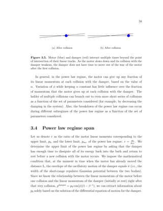
Figure 3.6. The contour plots show the numbers of elastic collisions in the power law
regime for α = 125, φ = 5◦, 0 < ξ < 2 and 250 < L
σ < 104. Notice that the largest
number of collisions is obtained for very large values of L
σ and ξ close to 1.
3.5 Physical systems
The features of the model that we developed in this section provide guidance for
the design criteria necessary in crafting eligible atomistic structures for a motor
that might show a power law decay of its momentum and energy in time. An
example of a class of physical systems with geometry and properties compatible to
the set up and the assumptions of our model is the class of double-walled carbon
nanotubes (DWCN).
Carbon nanotubes, in general, have already shown potential to function as
nanomotors [42–44] or oscillators [45, 46]. Over the years, experimentalists have
successfully controlled the lengths and the diameters of these systems. They can
reach lengths of milimeters, or even centimeters, and diameters of tens of nanome-
ters. In particular, incommensurate DWCN exhibit the property of superlubricity
(i.e., low friction) between their walls [47,48]. In this case, the potential corruga-
tion between the concentric walls of the nanotube is small (less than 1 meV/atom)
and the tubes can slide easily along each other. As far as their dynamics are

77. 62
concerned, several studies show that the tubes can oscillate relative to each other,
along their longitudinal axes, at frequencies in the gigahertz range [46,49].
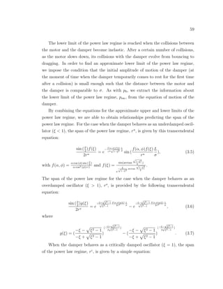
Figure 3.7. The outer tube (i.e., the motor) oscillates along its axis relative to the inner
tube and loses momentum via linear and periodic collisions with a small damper. The
damper is directly coupled to the thermal bath (i. e., the inner tube), where it dissipates
the energy gained from the motor.
Since the friction between the walls of the carbon tubes can be negligible, this
may allow the introduction of additional local and well-controlled dissipation into
the system. For example, we can functionalize the inner tube (i.e., the stator) with
a small molecule or even an atom, which would play the role of the damper in the
analytical model (see Fig. 3.7). The oscillating outer tube (i.e., the motor) can
give up momentum or energy via linear and periodic collisions with the damper.
The inner tube would also play the role of the thermal bath where the damper
dissipates the energy gained after the collision with the outer tube. Also, the mass
of the motor could be a few orders of magnitude larger than that of the damper.
We did not carry out any molecular dynamics simulations on atomistic DWCN
structures in this study.
3.6 Conclusions
Most macroscopic motors are immersed in a continuum dissipative fluidic back-
ground, whereas isolated molecular-scale systems are essentially non-dissipative,
since all configurational degrees of freedom are explicit. The transition between

78. 63
these two regimes is unclear, and may take several distinct paths. For example,
if all background degrees of freedom are roughly equally important, then a transi-
tion from an implicit to an explicit dynamics may be best handled by introducing
fluctuation effects onto the continuum to account for the discrete nature of small
systems. However, if the underlying degrees of freedom within the continuum back-
ground occupy a hierarchy of importance, then an alternative means of handling
the transition presents itself: to take successive degrees of freedom out of the con-
tinuum background and into explicit equation of motion one at a time, beginning
from the most important such degree of freedom. Certain molecular motor sys-
tems may satisfy this criterion, if their structure is such that successive collisions
of the main motor degree of freedom with a well-defined substructure dominate
the environmental coupling.
We investigate a situation in which one degree of freedom is pulled out from
the thermal bath and given an explicit equation of motion, interposed between
the bath and the motor. We describe a regime in which the deceleration of an
unpowered motor, coupled to a thermal bath via an explicit degree of freedom,
follows a power law in time with universal exponent of t equal to -1, rather than a
standard exponential decay. We find that the span of the power law regime depends
only on four dimensionless parameters and it can cover up to a few hundred elastic
collisions between the motor and the damper.
Many natural complex phenomena, from real earthquakes, sand piles, and bio-
logical extinctions to stock market fluctuations and traffic jams, follow power laws
in time [50]. However, there is an important distinction between the mechanism of
power law decay that we see in our motor system, and mechanisms of power law
in other systems in nature. Here, a system with no intrinsic time scale displays a
power law decay in time. In other systems, power law time dependence character-
izes multi-time scale processes, such as intramolecular vibrational dephasing [51]
and neuronal response adaptation to stimuli [52].
In the future, it would be interesting to craft and to study real atomistic struc-
tures, guided by the features of the analytical model, to develop real molecular
motors for which energy and momentum decay following a power law in time.

79. Chapter 4
1-Adamantanethiolate monolayer
displacement kinetics follow a
universal form
4.1 Introduction
Self-assembled monolayers (SAMs) are surfaces self-limited to a single, and often
well-ordered in-plane, layer of molecules on a substrate [53]. They are prepared
by adding the solution of the desired molecules onto the substrate, where they
spontaneously self-organize, and washing off the excess. A variety of SAMs can be
formed, using different molecules and substrates. Alkane or cycloalkane molecules
functionalized with thiol head groups (i.e., -SH groups) on gold substrates are a
common example, due to the affinity of sulfur for gold. In these SAMs, the thiol
head groups bind strongly to the substrate, while the molecules pack together
tightly due to the van der Waals forces, but with enough mobility to anneal and
to order.
The patterning and functionalization of surfaces with self-assembled monolay-
ers facilitate the creation of complex well-ordered structures for biosensors [54],
biomimetics [55, 56], molecular electronics [57, 58] or lithography [59–62]. How-
ever, surface diffusion and contamination can hinder the creation of high-quality
structures, especially for lithographic techniques that require multiple deposition

80. 65
steps. Protective layers can assist in controlling deposition, if they can be easily
removed when desired, but otherwise remain impermeable during the fabrication
of surface-bound nanoscale assemblies.
Experimentalists in Paul Weiss’s laboratory showed that 1-adamantanethiolate
(AD) SAMs are labile and can be displaced by short-chain n-alkanethiolates [63].
Although such displacement or exchange reactions are not unique to AD SAMs,
the complete and rapid displacement of one SAM by another under gentle thermal
conditions (room temperature) and dilute concentrations (mM) is unusual [64–66].
The labile nature of AD SAMs makes possible micro-displacement printing, a
technique similar to micro-contact printing, but wherein the patterned molecules
displace an existing SAM in only stamped regions, and the remaining SAM acts as
both a place-holder and a diffusion barrier [60,61]. These diffusion barriers not only
create sharper, higher quality patterns, but also extend the library of patternable
molecules to those otherwise too mobile to retain surface patterns. Despite the
recent interest in and multiple applications of AD SAMs, little is known about
the kinetics of AD SAM displacement. Understanding the displacement kinetics is
important both to achieve higher quality, reproducible chemically patterned films,
and to guide the design of new molecules for use as selectively labile monolayers.
With the help of spectroscopic methods, Paul Weiss’s lab showed that AD
and n-alkanethiolate SAMs have similar sulfur chemical environments [67], so the
displacement is not due to differences in Au–S bond strengths. Also, with the
help of scanning tunneling microscopy (STM), they found that n-alkanethiolate
SAMs are 1.8 times denser than AD SAMs [68]. They concluded that the complete
displacement of the AD SAMs is due to this density difference aided by differences
in van der Waals forces, which provide a substantial thermodynamic driving force.
They estimated that, based only on the energy of breaking/forming a S–Au bond,
the replacement of an AD SAM with an ALK SAM results in a gain of about
35.2 Kcal/mole of AD displaced. Also, using the measured interaction energy of
22.37 Kcal/mole for a C12 SAM, the replacement of an AD SAM with an ALK
SAM would result in a intermolecular interaction energy gain between 17.9 and
40.3 Kcal/mole of AD replaced.
Imaging with STM revealed that displacement begins with a rapid nucleation
phase, where n-dodecanethiolate (C12) molecules insert at defect sites of the AD

81. 66
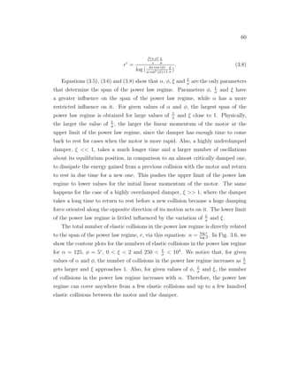
Figure 4.1. A) Schematic representation of the displacement of AD molecules by
C12 molecules. n-dodecanethiolate (C12) molecules insert at defect sites of the AD
SAM during a rapid nucleation phase. B) STM image of the real process: the (C12)
islands grow radially into domains that coalesce and eventually fully displace the original
monolayer.
SAM, followed by radial growth into domains that coalesce and eventually fully
displace the original monolayer [69]. The defects consist of both randomly dis-
tributed single-atom-deep vacancy islands in the gold substrate (from lifting the
Au{111} surface reconstruction during self-assembly) [70–72] and rotational/tilt
domain boundaries in the original SAM. Figure 4.1 shows a schematic representa-
tion of the displacement of the AD molecules by the C12 molecules and an STM
image of the real process.
In order to study the quantitative kinetics of the solution-phase displacement of
AD SAMs by C12 on Au{111}, they used Fourier transform infrared spectrometry
(FTIR). Below, we present briefly the experimental results of our collaborators.
For a more detailed description of the experimental methods and results, we direct
the reader to the article we published together with our collaborators [73].
4.2 Experimental results
The experimental procedure comprises several steps. First, the experimentalists
fabricate the AD SAMs by immersing flame-annealed Au{111} on mica substrates
into ethanolic solutions of 1-Adamantanethiol molecules with concentrations of
10 mM. After 24 hr deposition from solution, the gold substrates are removed,
rinsed with ethanol, and dried under a stream of nitrogen. The newly created
AD SAMs are investigated immediately after preparation, in order to asses their

82. 67
0.0000
0.0005
0.0010
0.0015
0.0020
2800 2850 2900 2950 3000
2850
2877
2911
2919
2935
2934
2963
2850
1-adamantanethiolate
n-dodecanethiolate
Wavenumber (cm-1)
Absorbance(a.u.)
Figure 4.2. Infrared spectra of the C-H stretch region of a AD SAM (black) and a
C12 SAM (grey), showing their spectral overlap.
quality. Preliminary FTIR spectra are acquired to verify the absence of impurity-
related features and the presence of the CH2 stretch at 2911 ± 1 cm−1
, both
indicative of a well-ordered AD SAM [69,74].
Next, they place the well-ordered AD SAMs in ethanolic C12 solutions of
specified concentration in order to achieve displacement. Every six minutes, the
SAMs are removed from solution, rinsed with ethanol and dried with nitrogen, a
FTIR spectrum is recorded, and the sample is returned to C12 solution for the
next incremental exposure. Displacements are no longer incrementally monitored
once the signals plateau; instead, the samples are placed in C12 solution overnight
to allow slow reordering and annealing and thereby achieve saturation coverage.
They obtain the infrared spectra of the adsorbed species on substrates from
400 to 4000 cm−1
. The region from 2800 to 3000 cm−1
contains the CH2 and CH3
stretch modes of the aliphatic and carbon-cage tails of the thiolated molecules.
Figure 4.2 shows the typical spectra of an AD SAM (black) and a C12 SAM
(grey), both recorded after 24 hr deposition. Several absorption peaks overlap in
this region: CH2 symmetric stretches (2850 cm−1
for both AD and C12 SAMs)
and CH2 asymmetric stretches (2911 cm−1
for AD SAMs and 2919 cm−1
for C12
SAMs) [74]. The peaks that do not overlap correspond to the CH3 symmetric and
asymmetric stretching modes of the C12 SAM, at 2877 and 2963 cm−1
, respectively
[75].

83. 68
0.000
0.005
0.010
0.015
0.020
0.025
0.030
0.035
2850 2900 2950 3000 30502800
Absorbance(a.u.)
Wavenumber (cm-1)
0 20 40 60 80 100
0.000
0.001
0.002
0.003
0.004
0.005
0.006
0.007
IntegratedAbsorbance(a.u.)
Exposure Time (min)
0 min
18 min
36 min
54 min
A B
Figure 4.3. A) Representative FTIR spectra of a 0.11 mM C12 solution displacing
an AD SAM. The 2877 cm−1 peak, corresponding to the CH3 symmetric mode, is
highlighted. B) A kinetic curve derived from the FTIR spectra by plotting the integrated
C12 CH3 symmetric mode peak versus deposition exposure time. The open squares
represent the integrated absorbance for each of the four spectra shown on the left.
These spectra provide peak intensities and peak positions as a function of im-
mersion time and solution concentration for two experimental trials per concentra-
tion. Figure 4.3A displays four spectra obtained at increasing immersion times in
a 0.11 mM C12 solution; each is a sum of contributions from both AD and C12.
Figure 4.3B plots the integrated 2877 cm−1
peak intensity as a function of exposure
time. Molecular orientation and lattice crystallinity affect the spectrum; for exam-
ple, shifts in the CH2 asymmetric mode track monolayer order and crystallinity.
However, the symmetric and asymmetric CH3 stretching modes are not sensitive
to the orientation of the C12 molecule, because of the tetrahedral coordination of
the three relevant hydrogens. Therefore, the strength of the symmetric CH3 mode
directly measures the C12 surface coverage [75]. As one can see in Fig. 4.3A, this
mode is initially very weak. After about 12 minutes of exposure to 0.11 mM C12,
the intensity of the 2877 cm−1
peak increases rapidly and eventually dominates
the spectrum. After 28 minutes, no signal from AD molecules can be detected
by FTIR and the spectrum is nearly identical to that of a pure C12 SAM. Dis-
placement becomes very slow at around 92% of the final saturation intensity and
approaches final saturation only after 24 hrs in solution. A similar but faster time
evolution is observed at higher displacement solution concentrations.

84. 69
4.3 Modelling of the kinetics of the displacement
process
In this section, we present the modelling of the kinetics of the displacement pro-
cess. Several experimental techniques [76–78] established that the growth rates
of alkanethiolate monolayers on bare Au{111} surfaces obey Langmuir kinetics
law, where the growth rates of adsorption are proportional to the number of un-
occupied adsorption sites on the surface. In our attempt to model the C12/AD
displacement kinetics, we consider several variants of the Langmuir model as eligi-
ble kinetics models, and in addition, a purely diffusion-controlled adsorption model
and two models based on island growth.
The simplest case, first-order Langmuir kinetics, is based on several assump-
tions: 1) all surface adsorption sites are equivalent; 2) a surface site is filled by
reaction with one molecule; molecules cannot adsorb in the regions around a site,
nor can multilayers form; 3) the number of sites remains unchanged during the re-
action; 4) there are no lateral molecular interactions, no interactions between the
adsorbing molecules and the pre-adsorbed ones nor the solvent molecules; and 5)
temperature is constant. The consequence of some of these assumptions is that the
adsorption rate is uniform across the entire available surface. By integrating the
relationship between the adsorption rate and the number of unoccupied adsorption
sites on the bare surface, dθ
dt
= κ(1 − θ), one obtains [79]:
θ(t) = 1 − e−κt
, (4.1)
where θ is the time-dependent surface coverage and κ is the rate constant.
Despite its simplicity, first-order Langmuir kinetics describes monolayer uptake
curves on bare gold surfaces fairly well. It has also been used to model the molec-
ular exchange of n-octadecanethiolate SAMs by radiolabeled n-octadecanethiol
molecules, although the reaction took 50 hrs and reached only ∼60% comple-
tion [66]. If the onset of surface coverage growth is delayed, then a time offset can
be introduced into the Langmuir equation above: θ(t) = 1 − e−κ(t−tc)
[80,81].
First-order Langmuir kinetics has been extended to account for diffusion-limited
kinetics [82], second-order processes [64, 82] and intermolecular interactions [83].

85. 70
When growth is limited by the diffusion of the molecules from the bulk solution to
the surface, one obtains the square-root time dependence associated with molecular
diffusive random walks:
θ(t) = 1 − e−
√
κt
. (4.2)
The diffusion-limited Langmuir model has been used successfully to describe the
adsorption kinetics of alkanethiol molecules on bare gold surfaces from very dilute
solutions ( 100 µM) [84].
If the rate of adsorption is second-order in the thiol concentration, the analytical
expression for the growth of the surface coverage over time becomes:
θ(t) = 1 −
1
1 + κt
. (4.3)
Second-order Langmuir adsorption kinetics has been used to describe ligand-exchange
reactions on ligand-stabilized nanoparticles. The rate of the reaction was taken to
depend on the concentration of the exchanging thiol both in solution and on the
surface [64].
For the purely diffusion-controlled adsorption, the time-dependent coverage
follows from the solution of the diffusion equations for a semi-infinite medium
[66,85]:
θ(t) =
√
κDt, (4.4)
where
κD =
4D
πB2
ml
, (4.5)
D is the diffusion constant and Bml is the number of molecules per unit area in the
full monolayer. The rate of adsorption is then proportional to the flux of molecules
to the surface. Since this model does not account for saturation or the depletion
of adsorption sites, it could only apply to the initial stages of growth.
The kinetics of phase transformations that occur via nucleation and island
growth were first modeled by Johnson, Mehl, Avrami and Kolmogorov (JMAK) in
the 1940s to describe metal alloy phase transformations [86–89].

86. 71
The JMAK model was originally derived in the framework of the following ex-
perimentally supported assumptions: 1). the nuclei are distributed randomly and
uniformly throughout the volume or the surface of the system wherein the phase
transformation occurs; 2). the growth rates of the newly formed grains/islands are
constant in time and uniform in all spatial directions; 3). growth ceases wherever
adjacent grains/islands impinge on each other; 4). the volume within which the
phase transformation occurs is infinite, there are no effects associated with finite
boundaries. The second assumption is equivalent to the assumption that the rate
at which the total transformed volume or surface grow is proportional to the total
surface area of the grains or the total perimeter of the islands, respectively.
The total number of nuclei distributed randomly and uniformly throughout
the volume/surface of the old phase changes as the phase transformation pro-
ceeds. Some of them start growing while others get swallowed up by the growing
islands of the new phase. Avrami finds that the time-dependent total transformed
volume/surface of the newly formed phase, V (t), can be expressed as a functional
of the number of nuclei, N(t), i.e., V (t) = V [N(t)] [86, 87]. Thus, at any time t,
the total transformed volume depends upon the values of N throughout the entire
time interval [0, t]. The functional can be then expanded as a Taylor series of sim-
ple functionals of different orders: linear, quadratic etc. The physical significance
of the various order terms in the series expansion can be extracted if one considers
a system in which the nuclei give rise to islands that grow unimpeded by other
neighboring growing islands. Because the islands overlap, the total transformed
volume obtained by summing over all the islands, called the ’extended’ volume, Ve,
overestimates the actual total transformed volume. Ve represents the linear term
in the series expansion of V [N(t)].
Let us denote V1 to be the transformed volume lying solely in the nonoverlap-
ping regions of Ve, V2 as the transformed volume lying solely in double overlapping
regions and so on. Both V and Ve can be expressed as a function of the volumes
corresponding to n-overlapping regions as follows:
V = V1 + V2 + ... + Vn + ..., (4.6)
Ve = V1 + 2V2 + ... + nVn + ... (4.7)

87. 72
After lengthy calculations, Avrami proves that the time-dependent total trans-
formed volume/surface of the newly formed phase, V (t), can be expressed using of
the total extended transformed volume, Ve, via this relationship: V (t) = 1−e−Ve(t)
.
Next, the extended transformed volume can be easily evaluated by using the rates
of nucleation and growth for the physical system at hand, and is found to have the
following form: Ve(t) = (κt)n
, where κ and n are constants.
The JMAK equation relates the evolution in time of the macroscopic fraction
of the newly formed phase (in our case, the C12 SAM surface coverage), with the
microscopic mechanisms of nucleation and growth:
θ(t) = 1 − e−(κt)n
, (4.8)
where κ is the rate constant of the transformation (in our case, the rate of displace-
ment). The Avrami exponent, n, reflects the dimensionality of the system and the
time dependence of the nucleation: n=2 for a two-dimensional system wherein nu-
cleation proceeds rapidly to completion (site-saturated nucleation, JMAK2), and
n=3 for a two-dimensional system wherein the nucleation rate is constant in time
(constant-rate nucleation, JMAK3). In JMAK3, more nucleation sites become
available as the transformation proceeds, such as in certain glass ceramics [90].
The JMAK model has later been extended to address heterogeneous nucleation
[91], non-uniform island growth rates [92, 93], and boundary constraints [94–96],
and has been applied to describe a variety of physical systems including oxidizing
metal surfaces [97,98], graphite-diamond transformations [99], and the crystalliza-
tion of thin films [100] or proteins [101].
Figure 4.4 shows least-squares fits of several different kinetic models to the
C12 coverage versus exposure time for a 0.01 mM C12 displacement solution.
Notice that of all the kinetic models considered, only JMAK2 (Eqn. (4.8) with
n = 2) fits the data. A similar conclusion applies across the full range of all C12
concentrations studied, from 0.01 to 1.0 mM, as shown in Fig. 4.5.
Although the diffusion-limited models successfully described the growth of
n-alkanethiolate from very dilute solutions onto bare gold surfaces [76], they do
not fit the experimental surface coverage curves for our physical system, where
adsorption occurs on a slower time scale (minutes as opposed to seconds) and the
solution concentrations are much higher (mM as opposed to µM).

88. 73
pure diffusion
first-order Langmuir
first order Langmuir (tc=23 min)
diffusion-limited Langmuir
second-order Langmuir
site-saturated nucleation JMAK2
constant-rate nucleation JMAK3
0 50 100 150 200 250 300 350
0.0000
0.0012
0.0025
0.0037
0.0050
0.0062
Exposure Time (min)
IntegratedAbsorbance(a.u.)
Figure 4.4. A representative 0.01 mM C12 uptake curve with least-squares fits to pure
diffusion (green), first-order Langmuir (purple), first-order Langmuir with an onset of
growth at 23 min (orange), diffusion-limited Langmuir (grey), second-order Langmuir
(black), site-saturated nucleation JMAK2 (red), and constant-rate nucleation JMAK3
(blue) models.
0 20 40 60 80
0.0
0.2
0.4
0.6
0.8
1.0
0.01 mM
0.035mM
0.11 mM
0.33 mM
0.55 mM
0.77 mM
1.00 mM
Exposure Time (min)
θC12
Figure 4.5. n-Dodecanethiolate monolayer formation by the displacement of an AD
SAM as a function of concentration. Solid lines are least-squares fits based on the site-
saturated nucleation model JMAK2 (Eqn. (4.8) with n=2).
The failure of Langmuir-based models, wherein adsorption is equally probable at all
unoccupied sites, is consistent with the STM observations that adsorption begins
at defect sites (i.e., not within the interiors of AD domains) and then proceeds at
the AD-C12 domain boundaries [69]. The rapid nucleation across these preexist-
ing active sites accounts for the success of JMAK2 over JMAK3.

89. 74
-2.0 -1.5 -1.0 -0.5 0.0
-2.2
-2.0
-1.8
-1.6
-1.4
-1.2
-1.0
-0.8
Log[κ(min-1)]
Log[ C12 Concentration (mM) ]
log κ = 0.5 log[C12] - 1.0
Figure 4.6. The displacement rate constant versus C12 concentration on a logarithmic
scale. The slope of 0.50 ± 0.05 implies that the rate constant is proportional to the
square-root of the C12 concentration.
Although several elaborations upon JMAK2 (incorporating boundary effects or
non-uniform growth rates) could be derived, such subtle distinctions are not re-
solved by the experimental data.
The fits to JMAK2 also provide a measure of the displacement rate constant κ
for each C12 concentration. Figure 4.6 plots the logarithm of κ for all experimen-
tal trials against the logarithm of the C12 solution concentration. The slope of
0.50 ± 0.05 suggests that the displacement rate is proportional to the square-root
of the C12 solution concentration, assuming that the density of nucleation sites
is roughly constant across all samples. This result is surprising, since insertion
and displacement is expected to be a unimolecular process (a bimolecular process
would yield a slope of two, not one-half). Half-order kinetics can arise, for exam-
ple, when the displacement of Y by X actually proceeds by the decomposition of
a predominant bimolecular state X2 that generates X. In our case, the half-order
kinetics suggests that the thiol ends of two adjacent C12 molecules might stick
together in solution, before displacing the AD molecules on the surface.
In addition to specific conclusions regarding the relative quality of fits to differ-
ent kinetic models, one can also analyze the displacement curves on a model-free
basis, to extract powerful general conclusions regarding the number and character
of any component sub-processes. Consider a general physical process as a compo-

90. 75
0 0.750.25 0.5 1.0
0.0
0.2
0.4
0.6
0.8
1.0
0.01 mM
0.03 mM
0.11 mM
0.33 mM
0.55 mM
0.77 mM
1.00 mM
Reduced Exposure Time
θC12
Figure 4.7. A plot of coverage versus reduced exposure time of two experimental runs at
each C12 concentration (0.01, 0.03, 0.11, 0.33, 0.55, 0.77 and 1.0 mM), showing collapse
onto a universal curve.
sition of multiple sub-processes, each having a unique characteristic time scale or
length scale, such as, the growth of a tree across diurnal and annual cycles, from a
smooth-skinned narrow sapling to a wider mature state with regular cracks in its
bark. When observing only a time-lapse movie of the tree’s growth, one can imme-
diately determine the frame rate and zoom factor: the faster cycle can be used as
a clock to pace the slower process, and the finer details can be used to measure out
the coarser features. However, if a physical process is governed by a single time
scale (i.e., one rate constant) and a single length scale (i.e., a density of nucleation
sites), then the physical system, considered in isolation, has no intrinsic clocks or
rulers. In mathematical terms, the curves describing the kinetics of a scale-free
process can be collapsed onto a single universal curve by a simple rescaling of the
time and space (in this case, areal coverage) axes. In physical terms, from just the
shape of a C12 displacement curve, one can surmise nothing about the density of
nucleation sites or the rate of displacement.
Figure 4.7 demonstrates, on a model-free basis, that the displacement of AD
by C12 is to a good approximation a scale-free process, governed by a single rate
constant and a single characteristic length scale. Upon rescaling the time and
coverage axes, the data across a hundred-fold range of C12 concentration collapse
onto a single universal curve. For convenience, this rescaling uses the JMAK2 rate

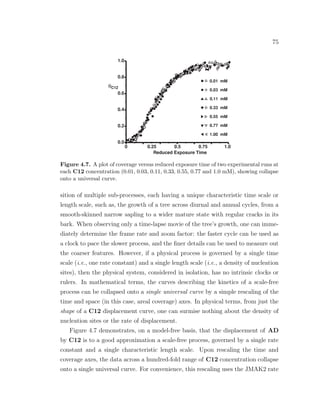
91. 76
constants, but as mentioned above, this scale-free universal behavior is model-
independent. The crystallization of metal alloys [86], the growth of diamond on
deformed silicon surface [102], or the oxidation of nickel surface [97,98] are other
examples of scale-free processes.
4.4 Conclusions
n-Dodecanethiol molecules in solution displace 1-adamantanethiolate self-assembled
monolayers on Au{111}, leading to complete molecular exchange. Fast insertion of
n-dodecanethiolate at defects in the original 1-adamantanethiolate monolayer nu-
cleates an island growth phase, which is followed by an eventual slow ordering of the
n-dodecanethiolate domains into a denser and more crystalline form. Langmuir-
based kinetics, which describe alkanethiolate adsorption on bare Au{111}, fail to
model this displacement reaction. Instead, a Johnson-Mehl-Avrami-Kolmogorov
model of perimeter-dependent island growth yields good agreement with exper-
imental data obtained over a hundred-fold variation in n-dodecanethiol concen-
tration. Rescaling the growth rate at each concentration collapses all the data
onto a single universal curve, suggesting that displacement is a purely geometri-
cal, scale-free process. The rate of displacement varies as the square-root of the
n-dodecanethiol concentration across the 0.01–1.0 mM range studied.

92. Chapter 5
Lanthanide double-decker complexes
as potential rotary motors
5.1 Introduction
Planar organic ligands, such as porphyrin (Pr), phthalocyanine (Pc), and naph-
thalocyanine (Nc) form complexes with metal ions, wherein the metal lies between
two ligands, known as metal double-decker complexes (DD). These structures have
important applications as sensors [103], molecular memory [104], and rotary mo-
tors [105].
X-ray diffraction analysis [106,107] reveals that lanthanide double-decker com-
plexes have sizes of 1-2 nm. Ring-to-ring separations between the internal faces of
the ligands vary between 2 ˚A and 3 ˚A, depending on the type of ligand and metal
ion. Strong π-π interaction between ligands results in staggered DD conformations,
with twist angles of 45◦
between the rings.
Aida and co-workers were the first to control the rate of rotation, to produce a
rotary motor capable of more than one speed [105,108]. They used a bisporphyri-
nate double-decker complex, with a cerium or zirconium ion sandwiched between
the two Pr ligands, that rotate with respect to one another. They found rotational
rates on the order of 10−6
to 10−4
Hz. Also, they discovered that, by reducing the
cerium complex led to the rotation of the Pr ligand being accelerated more than
300-fold.

93. 78
Oxidation of the zirconium complex, decelerated the rotation of the Pr ligand by
a factor of 21 or 99, depending on the oxidation state of the complex.
Experimentalists in Paul Weiss’s lab at Penn State investigated the potential
of lanthanide DD complexes to function as rotary motors. They developed and
applied design rules that enabled precise control over adsorption orientation and
spacing of lanthanide DD molecule arrays on substrates. They selectively attached
certain ligands within DD molecules to the graphite surface and oriented the coun-
terpart ligands off the surface [109,110]. Also, they controlled the intermolecular
distances between neighboring DD molecules on surface by varying the size of the
ligands adsorbed to the surface and by coadsorbing DD molecules with single-
ligand molecules [111]. In a DD rotary motor attached to a substrate, the metal
ion plays the role of the shaft of the motor, while the upper and the lower ligands
represent the rotor and the stator, respectively. Scanning tunneling microscopy
studies are yet to observe upper ligand rotation in any of the structures analyzed.
Our goal is to calculate the barriers to rotation for individual DD molecules
investigated by experimentalists, in an attempt to evaluate their potential as rotary
motors.
5.2 Barriers to rotation for lanthanide DD
complexes using DFT
In this section, we present the results for barriers to rotation for several different
DD molecules using DFT. We consider a luthetium metal ion and the following
combinations of ligands with no side-substituents: Pr/Pc (i.e., (Pr)Lu(Pc)), Pr/Nc
(i.e., (Pr)Lu(Nc)), Pc/Pc (i.e., (Pc)Lu(Pc)) and Pc/Nc (i.e., (Pc)Lu(Nc)).
Figures 5.1 and 5.2 show schematic representations of (Pc)Lu(Pc) and (Pr)Lu(Nc)
structures, respectively.
In order to calculate the barriers to rotation, we first optimize the DD molecules.
We find that the minimum energy structures correspond to staggered conforma-
tions with a twist angle of 45◦
for all structures investigated. Next, we calculate
the energies of the eclipsed conformations, which correspond to a skew angle of 0◦
.
The energy barriers to rotation are obtained as the difference in energy between

94. 79
Figure 5.1. Schematic representation of a double-decker rotary motor consisting of a Lu
ion sandwiched between two Pc ligands. The metal ion plays the role of the motor shaft,
while the upper and the lower ligands represent the rotor and the stator, respectively.
Figure 5.2. Schematic representation of a double-decker rotary motor consisting of a
Lu ion sandwiched between a Pr ligand (upper) and a Nc ligand (lower). The metal ion
plays the role of the motor shaft, while the upper and the lower ligands represent the
rotor and the stator, respectively.
the eclipsed and the staggered conformations. We find an energy barrier to rota-
tion of 0.79 eV for (Pr)Lu(Pc) (see Fig. 5.3). The intraplanar distance between
Pr and Pc ligands in staggered conformation is 2.71 ˚A, calculated as the distance
between the planes determined by the four central nitrogen atoms of each ligand.
The N–Lu bond lengths for the Pr and Pc ligands are 2.42 ˚A and 2.51 ˚A, respec-
tively. The Lu ion lies closer to Pr because it has a larger cavity (3.0 ˚A × 3.0 ˚A)
compared to Pc (2.9 ˚A × 2.9 ˚A), as determined by the N atoms of each ligand.
For (Pr)Lu(Nc), the energy barrier is only 1.7 meV larger. The replacement of Pc

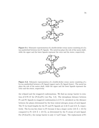
95. 80
(a) (b)
Figure 5.3. Staggered conformation of optimized (Pr)Lu(Pc) double-decker complex
using DFT. (a) Side view. (b) Top view. Atom colors are as follows: Lu yellow, N blue,
C and H green.
ligand with Nc does not give rise to a significant change in the energy barrier to
rotation. The outer Nc rings are situated too far away from the upper ligand, and
do not contribute to their mutual π-π interactions.
Similarly, the barriers to rotation for (Pc)Lu(Pc)) (see Fig. 5.4) and (Pc)Lu(Nc))
are almost equal, i.e., 0.94 eV. The intraplanar distance between the Pc ligands
in staggered conformation is 2.71 ˚A, calculated as the distance between the planes
determined by the central nitrogen atoms of each ligand. The N–Lu bond lengths
are 2.44 ˚A, with Lu ion at the same distance from each of the two Pc ligands.
The barriers to rotation of these Lu DD complexes are substantial and allow
only thermally activated hopping between adjacent staggered configurations of
the DD structures. By assuming an average value of −20 cal/mol/K [103] for the
activation entropy between the staggered and eclipsed conformations, and using the
Arrhenius formula (i.e., r = ωe
− ∆G
kBT
, with r, the rate of rotation, ω, the attempt
frequency, and ∆G, the activation free energy.), we estimate thermal rotational
rates on the order of 10−8
to 10−5
Hz at room temperature.
As a result of lanthanide contraction, we expect to obtain smaller barriers
to rotation when Lu is replaced by other lanthanide metal ions. However, the
optimization of DD complexes with lanthanide metal ions other than Lu proves
challenging, due to their incomplete 4f shell. In particular, it is rather difficult to
achieve electron density convergence for these systems. For example, the electron

96. 81
(a) (b)
Figure 5.4. Staggered conformation of optimized (Pc)Lu(Pc) double-decker complex
using DFT. (a) Side view. (b) Top view. Atom colors are as follows: Lu yellow, N blue,
C and H green.
density of the system can oscillate between two different electron density values,
whithout ever converging. Such issues are studied by a branch of mathematics
called chaos theory, and several different methods have already been developed to
address convergence difficulties in metal complexes [112].
5.3 Conclusions
Our preliminary results show that, the rotational barriers for a variety of DD
molecules, with no side-substituents attached to the ligands, and a luthetium ion
as shaft, are substantial and allow rotation only via thermally activated hopping.
For the future, it would be interesting to study the variation of rotational barriers
with size of the metal ion and its oxidation state, and size and position of ligand
side-substituents.
Experimentalists plan to continue their investigations of the rotation of DD
molecules with asymmetric rotors, which allow direct observation of the hopping
motion.

97. Bibliography
[1] Noji, H., R. Yasuda, M. Yoshida, and K. Kinosita (1997) “Direct
observation of the rotation of F1 − ATPase,” Nature, 386, p. 299.
[2] Yasuda, R., H. Noji, K. Kinosita, and M. Yoshida (1998) “F1 −
ATPase is a highly efficient molecular motor that rotates with discrete 120◦
steps,” Cell, 93, p. 1117.
[3] Schliwa, M. and G. Woehlke (2003) “Molecular motors,” Nature, 422,
p. 759.
[4] Kelly, T. R., H. D. Silva, and R. A. Silva (1999) “Unidirectional rotary
motion in a molecular system,” Nature, 401, p. 150.
[5] Green, J. E., J. F. Stoddart, and J. R. Heath (2007) “A 160-kilobit
molecular electronic memory patterned at 1011
bits per square centimetre,”
Nature, 445, p. 414.
[6] Bissell, R. A., E. Cordova, A. E. Kaifer, and J. F. Stoddart (1994)
“A chemically and electrochemically switchable molecular shuttle,” Nature,
369, p. 133.
[7] Berna, J. and F. Zerbetto (2005) “Macroscopic transport by synthetic
molecular machines,” Nature Materials, 4, p. 704.
[8] Koumura, N., R. Zijlstra, R. A. van Delden, N. Harada, and
B. Feringa (1999) “Light-driven monodirectional molecular rotor,” Nature,
401, p. 152.
[9] van Delden, R. A., M. ter Wiel, M. Pollard, J. Vicario,
N. Koumura, and B. Feringa (2005) “Unidirectional molecular motor
on a gold surface,” Nature, 437, p. 1337.

98. 83
[10] Vicario, J., M. Walko, A. Meetsma, and B. Feringa (2006) “Fine
tuning of the rotary motion by structural modification in light-driven unidi-
rectional molecular motors,” J. Am. Chem. Soc., 128, p. 5127.
[11] Kumar, A. S., T. Ye, T. Takami, B. Yu, A. K. Flatt, J. M. Tour,
and P. S. Weiss (2008) “Reversible photo-switching of single azebenzene
molecules in controlled nanoscale environments,” Nano Letters, 8, p. 1644.
[12] Troisi, A. and M. A. Ratner (2004) “Conformational molecular recti-
fiers,” Nano Letters, 4, p. 591.
[13] Shirai, Y. S., A. J. Osgood, Y. Zhao, K. F. Kelly, and J. M. Tour
(2005) “Directional control in thermally driven single-molecule nanocars,”
Nano Letters, 5, p. 2330.
[14] Takami, T., T. Ye, D. P. Arnold, K. Sugiura, R. Wang, J. Jiang,
and P. S. Weiss (2007) “Controlled adsorption orientation for double-decker
complexes,” J. Phys. Chem. C, 111, p. 2077.
[15] Khuong, T., J. Nunez, C. Godinez, and M. Garcia-Garibay (2006)
“Crystalline molecular machines: A quest toward solid-state dynamics and
function,” Acc. Chem. Res., 39, p. 413.
[16] Dominguez, Z., T. Khuong, H. Dang, C. Sanrame, J. Nunez, and
M. Garcia-Garibay (2003) “Molecular compasses and gyroscopes with
polar rotors: synthesis and characterization of crystalline forms,” J. Am.
Chem. Soc., 125, p. 8827.
[17] Garcia-Garibay, M. (2005) “Crystalline molecular machines: Encoding
supramolecular dynamics into molecular structure,” Proc. Natl. Acad. Sci.,
102, p. 10771.
[18] Vacek, J. and J. Michl (1997) “A molecular ”Tinkertoy” construction kit:
Computer simulation of molecular propellers,” New J. Chem., 21, p. 1259.
[19] Hohenberg, P. and W. Kohn (1964) “Inhomogeneous electron gas,” Phys.
Rev. B, 136, p. 864.
[20] Levy, M. (1982) “Electron densities in search of Hamiltonians,”
Phys. Rev. A, 26, p. 1200.
[21] Kohn, W. and L. J. Sham (1965) “Self consistent equations including
exchange and correlation effects,” Phys. Rev. A, 140, p. 1133.
[22] Ceperley, D. M. and B. J. Alder (1980) “Ground state of the electron
gas by a stochastic method,” Phys. Rev. Lett., 45, p. 566.

99. 84
[23] Becke, A. D. (1988) “Density-functional exchange-energy approximation
with correct asymptotic behavior,” Phys. Rev. A, 38, p. 3098.
[24] Lee, C., W. Yang, and R. G. Parr (1988) “Development of the Colle-
Salvetti correlation-energy formula into a functional of the electron density,”
Phys. Rev. B, 37, p. 785.
[25] Stephens, P. J., J. F. Devlin, C. F. Chabalowski, and M. J. Frisch
(1994) “Ab initio calculation of vibrational absorption and circular dichroism
spectra using density functional force fields,” J. Phys. Chem., 98, p. 11623.
[26] Koch, W. and M. C. Holthausen (2001) A chemist’s guide to density
functional theory, John Wiley & Sons, Weinheim.
[27] Rappe, A. K. and W. A. Goddard (1991) “Charge equilibration for
molecular dynamics simulations,” J. Phys. Chem., 95, p. 3358.
[28] Rappe, A. K., C. J. Casewit, K. S. Colwell, W. A. Goddard, and
W. M. Skiff (1992) “UFF, a full periodic table force field for molecular
mechanics and molecular dynamics simulations,” J. Am. Chem. Soc., 114,
p. 10024.
[29] Casewit, C. J., K. S. Colwell, and A. K. Rappe (1992) “Application
of a universal force field to organic molecules,” J. Am. Chem. Soc., 114, p.
10035.
[30] Casewit, C., K. S. Colwell, and A. K. Rappe (1992) “Application of
a universal force field to main group compounds,” J. Am. Chem. Soc., 114,
p. 10046.
[31] Rappe, A. K., K. S. Colwell, and C. J. Casewit (1993) “Application
of a universal force field to metal complexes,” Inorg. Chem., 32, p. 3438.
[32] Vacek, J. and J. Michl (2001) “Molecular dynamics of a grid-mounted
molecular dipolar rotor in a rotating electric field,” Proc. Natl. Acad. Sci.,
98, p. 5481.
[33] Horinek, D. and J. Michl (2003) “Molecular dynamics simulation of an
electric field driven dipolar molecular rotor attached to a quartz glass sur-
face,” J. Am. Chem. Soc., 125, p. 11900.
[34] Zheng, H., M. E. Mulcahy, D. Horinek, F. Galeotti, T. F. Mag-
nera, and J. Michl (2004) “Dipolar and nonpolar altitudinal molecular
rotors mounted on an Au(111) surface,” J. Am. Chem. Soc., 126, p. 4540.

100. 85
[35] Clarke, L. I., D. Horinek, G. S. Kottas, N. Varaksa, T. F. Mag-
nera, T. P. Hinderer, R. D. Horansky, J. Michl, and J. P. Price
(2002) “The dielectric response of chloromethylsilyl and dychloromethylsilyl
dipolar rotors on fused silica surfaces,” Nanotehnology, 13, p. 533.
[36] Kottas, G. S., L. I. Clarke, D. Horinek, and J. Michl (2005) “Arti-
ficial molecular rotors,” Chem. Rev., 105, p. 1281.
[37] Jian, H. and J. M. Tour (2003) “En route to surface-bound electric field-
driven molecular motors,” J. Org. Chem., 68, p. 5091.
[38] Schmidt, M. W., K. K. Baldridge, J. A. Boatz, S. T. Elbert, M. S.
Gordon, J. H. Jensen, S. Koseki, N. Matsunaga, K. A. Nguyen,
S. Su, T. L. Windus, M. Dupuis, and J. A. Montgomery (1993)
“General atomic and molecular electronic structure system,” J. Comput.
Chem., 14, p. 1347.
[39] Gordon, M. S. and M. W. Schmidt (2005) “Advances in electronic struc-
ture theory: GAMESS a decade later,” in Theory and applications of com-
putational chemistry: the first forty years (C. E. Dykstra, G. Frenking, K. S.
Kim, and a G. E. Scuseria, eds.), Elsevier, Amsterdam, p. 1167.
[40] Li, H. and H. Jensen (2002) “Partial Hessian vibrational analy-
sis: the localization of the molecular vibrational energy and entropy,”
Theor. Chem. Acc., 107, p. 211.
[41] Head, J. D. (1997) “Computation of vibrational frequencies for adsorbates
on surfaces,” Int. J. Quant. Chem., 65, p. 827.
[42] Tu, Z. C. and X. Hu (2005) “Artificial molecular motor constructed
from a double-walled carbon nanotube driven by axially varying voltage,”
Phys. Rew. B, 72, p. 33404.
[43] Srivastava, D. (1997) “A phenomenological model of the rota-
tion dynamics of carbon nanotube gears with laser electric fields,”
Nanotechnology, 72, p. 186.
[44] Fennimore, A. M., T. D. Yuzvinsky, W. Han, M. S. Fuhrer,
J. Cummings, and A. Zetti (2003) “Rotational actuators based on carbon
nanotubes,” Nature, 424, p. 408.
[45] Zhang, S., W. K. Liu, and R. S. Ruoff (2004) “Atomistic simulations
of double-walled carbon nanotubes as rotational bearings,” Nanoletters, 4,
p. 293.

101. 86
[46] Zheng, Q. and Q. Jiang (2002) “Multiwalled carbon nanotubes as giga-
hertz oscillators,” Phys. Rev. Lett., 88, p. 45503.
[47] Dienwiebel, M., G. S. Verhoeven, N. Pradeep, and J. W. M.
Frenken (2004) “Superlubricity of graphite,” Phys. Rew. B, 92, p. 126101.
[48] Kolmogorov, A. N. and V. H. Crespi (2000) “Smoothest bearings:
Interlayer sliding in multiwalled carbon nanotubes,” Phys. Rew. Lett., 85, p.
4727.
[49] Legoas, S. B., V. R. Coluci, S. F. Braga, P. Z. Coura, S. O. Dan-
tas, and D. S. Galvao (2004) “Gigahertz nanomechanical oscillators based
on carbon nanotubes,” Nanotechnology, 15, p. 184.
[50] Bak, P. (1996) How nature works: The science of self-organised criticality,
Copernicus Press, New York, NY.
[51] Gruebele, M. (1998) “Intramolecular vibrational dephasing obeys a power
law at intermediate times,” Proc. Natl. Acad. Sci., 95, p. 5965.
[52] Drew, P. and L. Abbott (2006) “Models and properties of power-law
adaptation in neural systems,” J. Neurophysiol., 96, p. 826.
[53] Schreiber, F. (2000) “Structure and growth of self-assembling
monolayers,” Prog. Surf. Sci., 65, p. 151.
[54] Huang, L., G. Reekmans, D. Saerens, J. M. Friedt, F. Frederix,
L. Francis, S. Muyldermans, A. Campitelli, and C. Van Hoof
(2005) “Prostate-specific antigen immunosensing based on mixed self-
assembled monolayers, camel antibodies and colloidal gold enhanced sand-
wich assays,” Biosensors & Bioelectronics, 21, p. 483.
[55] Kwok, C. S., P. D. Mourad, L. A. Crum, and B. D. Ratner (2000)
“Surface modification of polymers with self-assembled molecular structures:
Multitechnique surface characterization,” Biomacromolecules, 1, p. 139.
[56] Mullen, T. J., A. A. Dameron, A. M. Andrews, and P. S. Weiss
(2007) “Selecting and driving monolayer structures through tailored inter-
molecular interactions,” Aldrichimica Acta, 40, p. 21.
[57] Mantooth, B. A. and P. S. Weiss (2003) “Fabrication, assembly, and
characterization of molecular electronic components,” Proc. IEEE, 91, p.
1785.

102. 87
[58] Moore, A. M., A. A. Dameron, B. A. Mantooth, R. K. Smith,
D. J. Fuchs, J. W. Ciszek, F. Maya, Y. X. Yao, J. M. Tour,
and P. S. Weiss (2006) “Molecular engineering and measurements to
test hypothesized mechanisms in single molecule conductance switching,”
J. Am. Chem. Soc., 128, p. 1959.
[59] Anderson, M. E., M. Mihok, H. Tanaka, L. P. Tan, M. W.
Horn, G. S. McCarty, and P. S. Weiss (2006) “Hybrid approaches
to nanolithography: Photolithographic structures with precise, controllable
nanometer-scale spacings created by molecular rulers,” Adv. Mater., 18, p.
1020.
[60] Dameron, A. A., J. R. Hampton, R. K. Smith, T. J. Mullen,
S. D. Gillmor, and P. S. Weiss (2005) “Microdisplacement printing,”
Nano Lett., 5, p. 1834.
[61] Dameron, A. A., J. R. Hampton, S. D. Gillmor, J. N. Hohman, and
P. S. Weiss (2005) “Enhanced molecular patterning via microdisplacement
printing,” J. Vac. Sci. Technol. B, 23, p. 2929.
[62] Smith, R. K., P. A. Lewis, and P. S. Weiss (2004) “Patterning self-
assembled monolayers,” Prog. Surf. Sci., 75, p. 1.
[63] Dameron, A. A., L. F. Charles, and P. S. Weiss (2005) “Struc-
tures and displacement of 1-adamantanethiol self-assembled monolayers on
Au(111),” J. Am. Chem. Soc., 127, p. 8697.
[64] Kassam, A., G. Bremner, B. Clark, G. Ulibarri, and R. B. Lennox
(2006) “Place exchange reactions of alkyl thiols on gold nanoparticles,”
J. Am. Chem. Soc., 128, p. 3476.
[65] Lussem, B., L. Muller-Meskamp, S. Karthauser, R. Waser,
M. Homberger, and U. Simon (2006) “STM study of mixed alka-
nethiol/biphenylthiol self-assembled monolayers on Au(111),” Langmuir, 22,
p. 3021.
[66] Schlenoff, J. B., M. Li, and H. Ly (1995) “Stability and self-exchange
in alkanethiol monolayers,” J. Am. Chem. Soc., 117, p. 12528.
[67] Dameron, A. A., T. J. Mullen, R. W. Hengstebeck, H. M.
Saavedra, and P. S. Weiss (2007) “Origins of displacement in
1-adamantanethiolate self-assembled monolayers,” J. Phys. Chem. C, 111,
p. 6747.

103. 88
[68] Mullen, T. J., A. A. Dameron, and P. S. Weiss (2006) “Directed
assembly and separation of self-assembled monolayers via electrochemical
processing,” J. Phys. Chem. B, p. 14410.
[69] Mullen, T. J., A. A. Dameron, H. M. Saavedra, M. E. Williams,
and P. S. Weiss (2007) “Dynamics of displacement in 1-adamantanethiolate
self-assembled monolayers,” J. Phys. Chem. C, 111, p. 6740.
[70] Poirier, G. E. (1997) “Characterization of organosulfur molecular mono-
layers on Au(111) using scanning tunneling microscopy,” Chem. Rev., 97, p.
1117.
[71] ——— (1997) “Mechanism of formation of Au vacancy islands in alkanethiol
monolayers on Au(111),” Langmuir, 13, p. 2019.
[72] Poirier, G. E. and E. D. Pylant (1996) “The self-assembly mechanism
of alkanethiols on Au(111),” Science, 272, p. 1145.
[73] Saavedra, H. M., C. M. Barbu, A. Dameron, T. J. Mullen, V. H.
Crespi, and P. S. Weiss (2007) “1-Adamantanethiolate monolayer dis-
placement kinetics follow a universal form,” J. Am. Chem. Soc., 129, p.
10741.
[74] Jensen, J. O. (2004) “Vibrational frequencies and structural determination
of adamantane,” Spectrochim. Acta, Part A, 60, p. 1895.
[75] Nuzzo, R. G., L. H. Dubois, and D. L. Allara (1990) “Fundamental-
studies of microscopic wetting on organic-surfaces.1. Formation and struc-
tural characterization of a self-consistent series of polyfunctional organic
monolayers,” J. Am. Chem. Soc., 112, p. 558.
[76] Bain, C. D. and G. M. Whitesides (1989) “Formation of monolayers by
the coadsorption of thiols on gold - variation in the length of the alkyl chain,”
J. Am. Chem. Soc., 111, p. 7164.
[77] Thomas, R. C., L. Sun, R. M. Crooks, and A. J. Ricco (1991) “Real-
time measurements of the gas-phase adsorption of normal-alkylthiol mono-
layers and multilayers on gold,” Langmuir, 7, p. 620.
[78] Karpovich, D. S. and G. J. Blanchard (1994) “Direct measurement
of the adsorption-kinetics of alkanethiolate self-assembled monolayers on a
microcrystalline gold surface,” Langmuir, 10, p. 3315.
[79] Langmuir, I. (1918) “The adsorption of gases on plane surfaces of glass,
mica and platinum,” J. Appl. Phys., 40, p. 1361.

104. 89
[80] Eberhardt, A., P. Fenter, and P. Eisenberger (1998) “Growth ki-
netics in self-assembling monolayers: a unique adsorption mechanism,” Surf.
Sci., 397, p. 285.
[81] Schwartz, P., F. Schreiber, P. Eisenberger, and G. Scoles (1999)
“Growth kinetics of decanethiol monolayers self-assembled on Au(111) by
molecular beam deposition: An atomic beam diffraction study,” Surf. Sci.,
423, p. 208.
[82] Peterlinz, K. A. and R. Georgiadis (1996) “In situ kinetics of self-
assembly by surface plasmon resonance spectroscopy,” Langmuir, 12, p.
4731.
[83] Dannenberger, O., M. Buck, and M. Grunze (1999) “Self-assembly
of n-alkanethiols: A kinetic study by second harmonic generation,” J. Phys.
Chem. B, 103, p. 22023.
[84] Woodward, J. T., I. Doudevski, H. D. Sikes, and D. K. Schwartz
(1997) “Kinetics of self-assembled monolayer growth explored via submono-
layer coverage of incomplete films,” J. Phys. Chem. B, 101, p. 7535.
[85] Spinke, J., M. Liley, F. J. Schmitt, H. J. Guder, L. Angermaier,
and W. Knoll (1993) “Molecular recognition at self-assembled monolayers
- Optimization of surface functionalization,” J. Chem. Phys., 99, p. 7012.
[86] Avrami, M. (1939) “Kinetics of phase change I - General theory,” J. Chem.
Phys., 7, p. 1103.
[87] ——— (1940) “Kinetics of phase change II,” J. Chem. Phys., 8, p. 212.
[88] ——— (1941) “Kinetics of phase change III,” J. Chem. Phys., 9, p. 117.
[89] Johnson, W. A. and R. F. Mehl (1939) “Reaction kinetics in processes
of nucleation and growth,” Trans. Am. Inst. Min. Metall. Eng., 135, p. 416.
[90] Holand, W., V. Rheinberger, and M. Schweiger (2003) “Control of
nucleation in glass ceramics,” Philos. Trans. R. Soc. Lond. Ser. A-Math.
Phys. Eng. Sci., 361, p. 575.
[91] Weinberg, M. C., D. P. Birnie, and V. A. Shneidman (1997) “Crys-
tallization kinetics and the JMAK equation,” J. Non-Cryst. Solids, 219,
p. 89.
[92] Shneidman, V. A. and M. C. Weinberg (1993) “The effects of tran-
sient nucleation and size-dependent growth-rate on phase-transformation
kinetics,” J. Non-Cryst. Solids, 160, p. 89.

105. 90
[93] Weinberg, M. and R. Kapral (1989) “Phase-transformation kinetics in
finite inhomogeneously nucleated systems,” J. Chem. Phys., 91, p. 7146.
[94] Jun, S., H. Y. Zhang, and J. Bechhoefer (2005) “Nucleation and
growth in one dimension. I. The generalized Kolmogorov-Johnson-Mehl-
Avrami model,” Phys. Rev. E, 71, p. 11908.
[95] Kooi, B. J. (2004) “Monte Carlo simulations of phase transformations
caused by nucleation and subsequent anisotropic growth: Extension of the
Johnson-Mehl-Avrami-Kolmogorov theory,” Phys. Rev. B, 70, p. 224108.
[96] ——— (2006) “Extension of the Johnson-Mehl-Avrami-Kolmogorov theory
incorporating anisotropic growth studied by Monte Carlo simulations,” Phys.
Rev. B, 73, p. 54103.
[97] Holloway, P. H. and J. B. Hudson (1974) “Kinetics of reaction of oxygen
with clean nickel single-crystal surfaces. 1. Ni(100) surface,” Surf. Sci., 43,
p. 123.
[98] ——— (1974) “Kinetics of reaction of oxygen with clean nickel single-crystal
surfaces. 2. Ni(111) surface,” Surf. Sci., 43, p. 141.
[99] Okada, T., W. Utsumi, H. Kaneko, V. Turkevich, N. Hamaya, and
O. Shimomura (2004) “Kinetics of the graphite-diamond transformation in
aqueous fluid determined by in-situ X-ray diffractions at high pressures and
temperatures,” Phys. Chem. Miner., 31, p. 261.
[100] Ruitenberg, G., A. K. Petford-Long, and R. C. Doole (2002) “De-
termination of the isothermal nucleation and growth parameters for the crys-
tallization of thin Ge2Sb2Te5 films,” J. Appl. Phys., 92, p. 3116.
[101] Baird, J. K., S. C. Hill, and J. C. Clunie (1999) “Kinetics of protein
crystal nucleation and growth in the batch method,” J. Cryst. Growth, 196,
p. 220.
[102] Fanfoni, M. and M. Tomellini (1998) “The Johnson-Mehl-Avrami-
Kolmogorov model: a brief review,” Il Nuovo Cimento, 20, p. 1171.
[103] Ercolani, G. (2005) “The origin of cooperativity in double-wheel receptors.
Freezing of internal rotation or ligand-induced torsional strain?” Org. Lett.,
7, p. 803.
[104] Sugasaki, A., M. Ikeda, M. Takeuchi, A. Robertson, and S. Shinkai
(1999) “Efficient chirality transcription utilizing a cerium(IV) double decker
porphyrin: a prototype for development of a molecular memory system,” J.
Chem. Soc., 1, p. 3259.

106. 91
[105] Tashiro, K., K. Konishi, and T. Aida (2000) “Metal bisporphyrinate
double-decker complexes as redox-responsive rotating modules. Studies on
ligand rotation activities of the reduced and oxidized forms using chirality
as a probe,” J. Am. Chem. Soc., 122, p. 7921.
[106] Bian, Y., D. Wang, R. Wang, L. Weng, J. Dou, D. Zhao, D. Ng,
and J. Jiang (2003) “Structural studies of the whole series of lanthanide
double-decker compounds with mixed 2,3-naphthalocyaninato and octaethyl-
porphyrinato ligands,” New J. Chem., 27, p. 844.
[107] Bian, Y., R. Wang, D. Wang, R. Wang, P. Zhu, R. Li, J. Dou,
W. Liu, C. Choi, H. Chan, C. Ma, D. Ng, and J. Jiang (2004)
“Synthesis, structure, and spectroscopic and electrochemical properties
of heteroleptic bis(phthalocyaninato) rare earth complexes with a C4
symmetry,” Helv. Chim. Acta, 87, p. 2581.
[108] Tashiro, K., K. Konishi, and T. Aida (1997) “Enantiomeric resolu-
tion of chiral metallobis(porphyrin)s: Studies on rotatability of electronically
coupled porphyrin ligands,” Angew. Chem. Int. Ed. Engl., 36, p. 856.
[109] Takami, T., D. Arnold, A. Fuchs, G. Will, R. Goh, E. Waclawik,
J. Bell, P. Weiss, K. Sugiura, W. Liu, and J. Jiang (2006) “Two-
dimensional crystal growth and stacking of bis(phthalocyaninato) rare earth
sandwich complexes at the 1-phenyloctane/graphite interface,” J. Phys.
Chem. B, 110, p. 1661.
[110] Takami, T., T. Ye, D. Arnold, K. Sugiura, R. Wang, J. Jiang,
and P. Weiss (2007) “Controlled adsorption orientation for double-decker
complexes,” J. Phys. Chem. C, 111, p. 2077.
[111] Ye, T., T. Takami, R. Wang, J. Jiang, and P. Weiss (2006) “Tuning
interactions between ligands in self-assembled double-decker phthalocyanine
arrays,” J. Am. Chem. Soc., 128, p. 10984.
[112] Strogatz, S. (2001) Nonlinear dynamics and chaos, John Wiley & Sons,
Boulder, Colorado.

107. Vita
Corina Madalina Barbu
Education
2008 Ph.D., Condensed Matter Physics, Pennsylvania State University
2000 M.S., Condensed Matter Physics, University of Bucharest
Awards
2008 Duncan Graduate Fellowship, PSU
2007 Duncan Graduate Fellowship, PSU
2006 Duncan Graduate Fellowship, PSU
2005 Duncan Graduate Fellowship, PSU
2002-2003 Braddock Graduate Fellowship, PSU