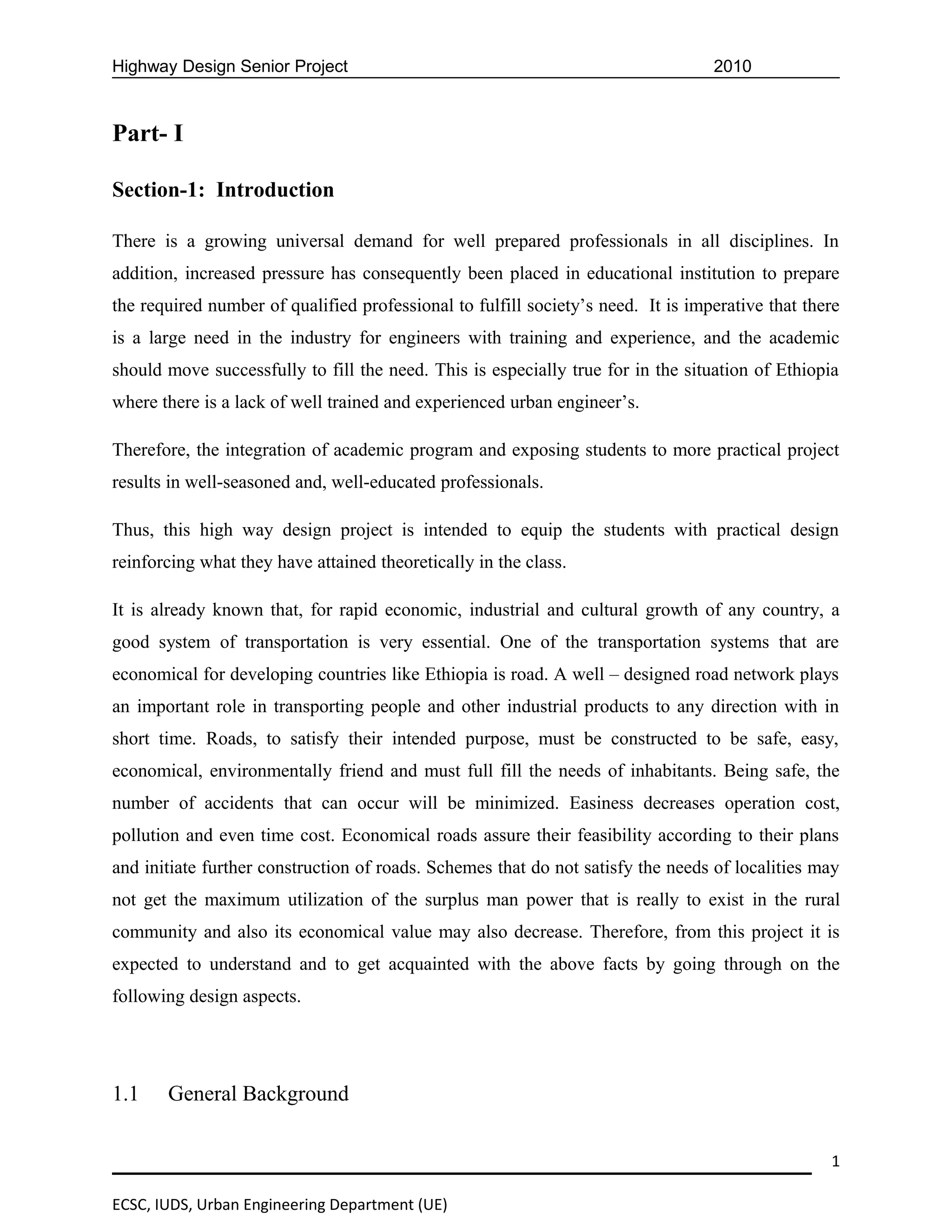
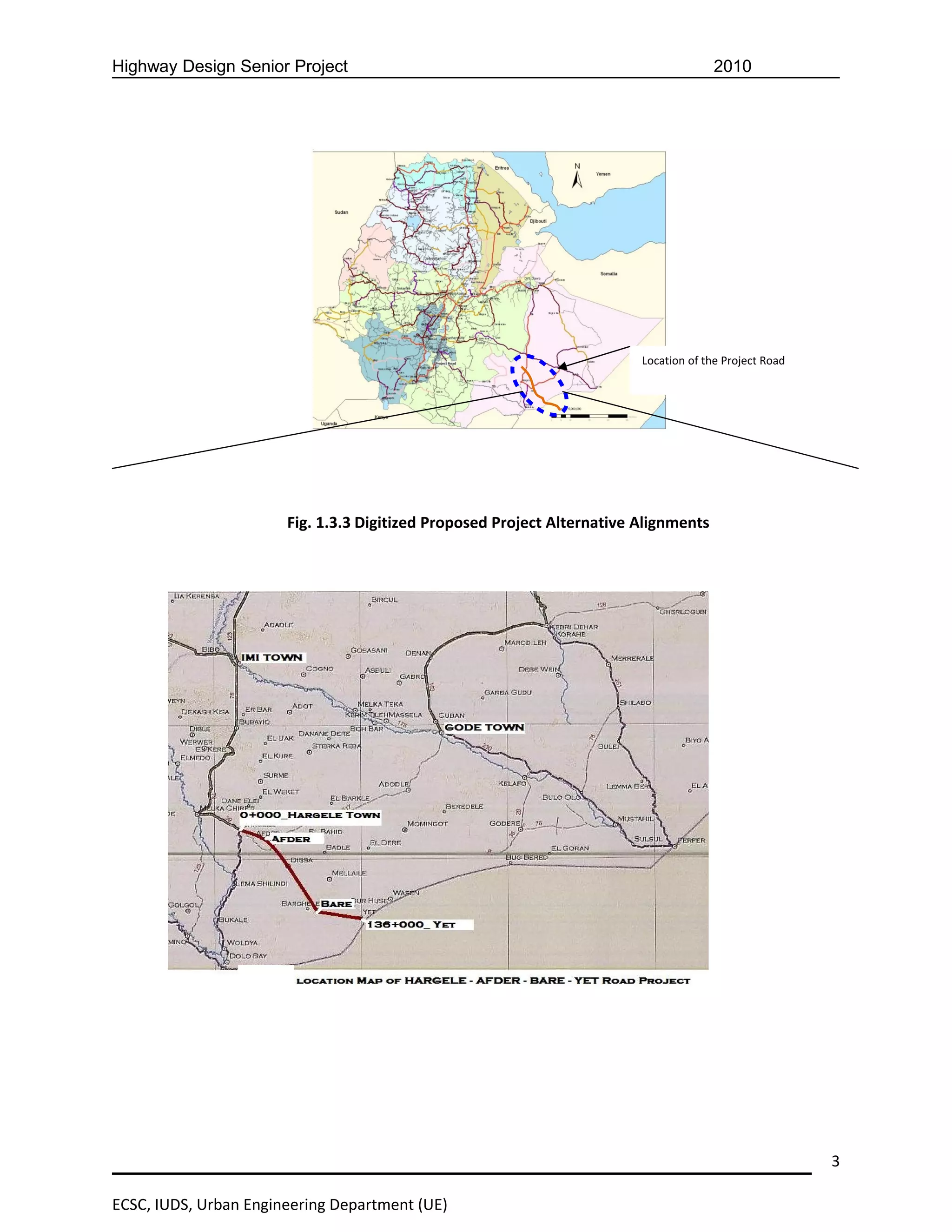
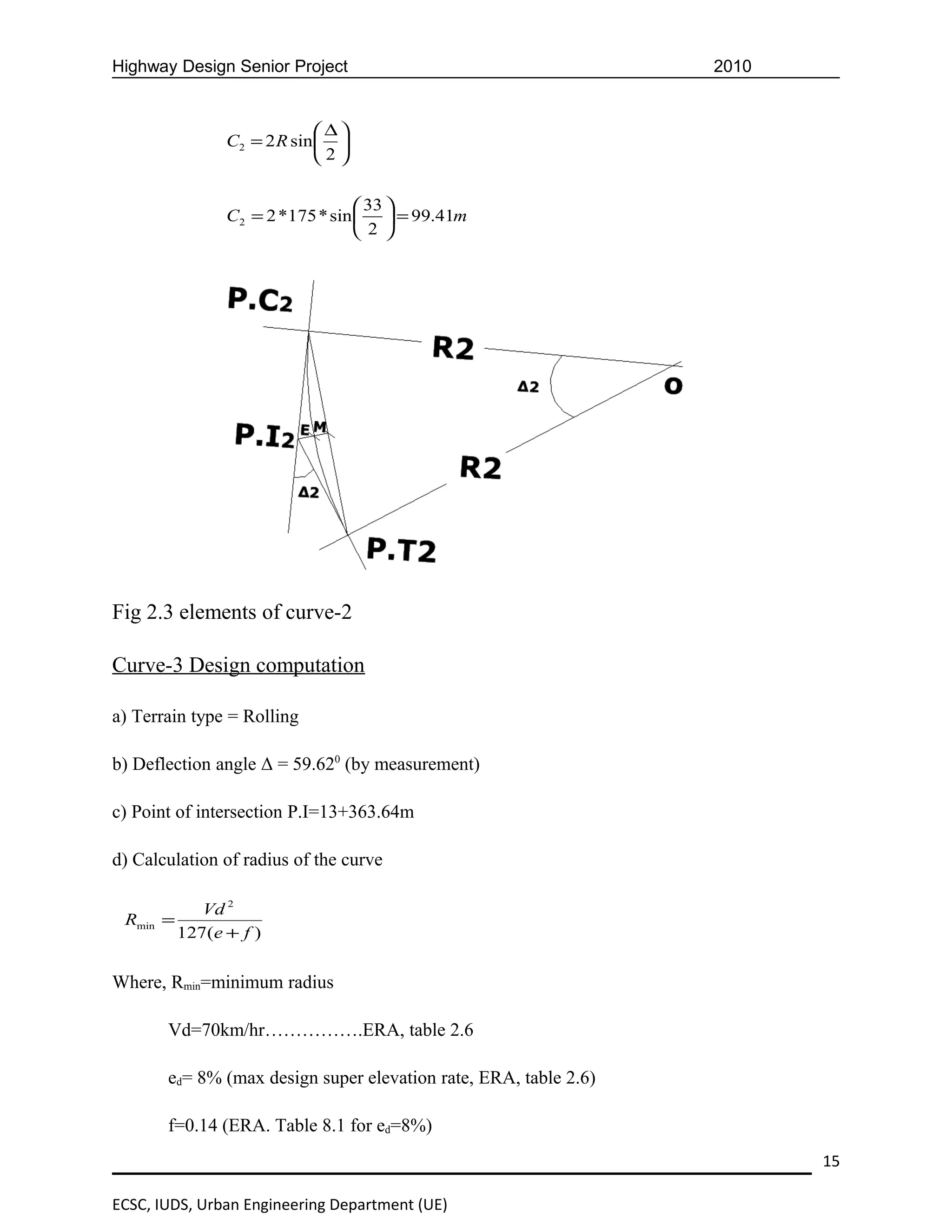
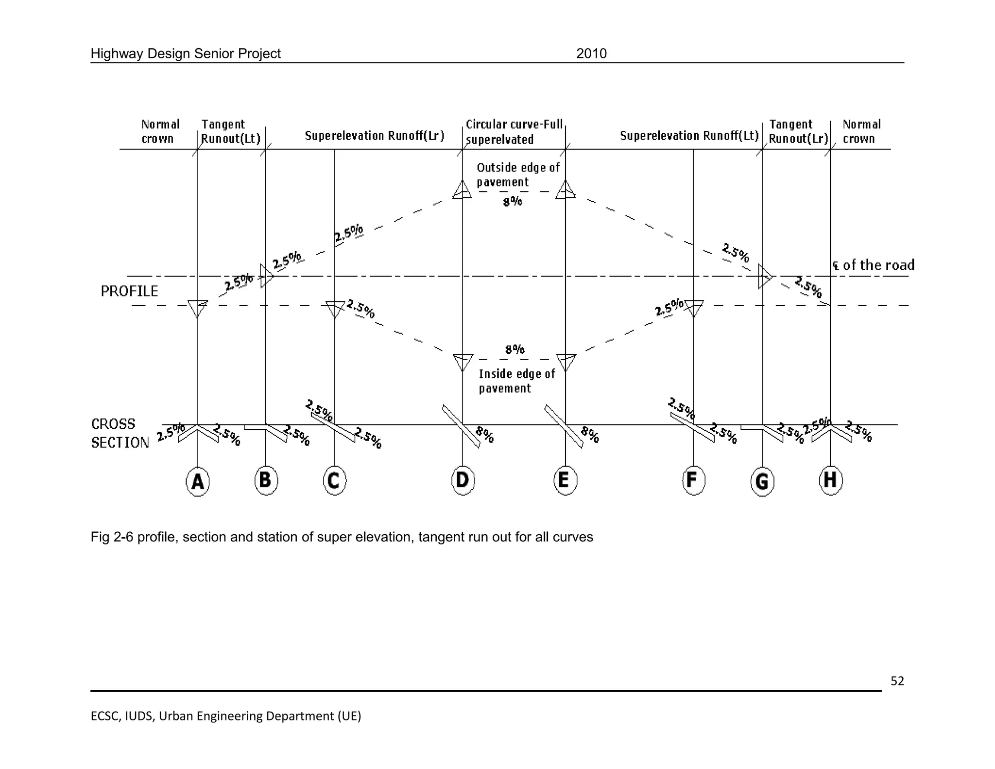
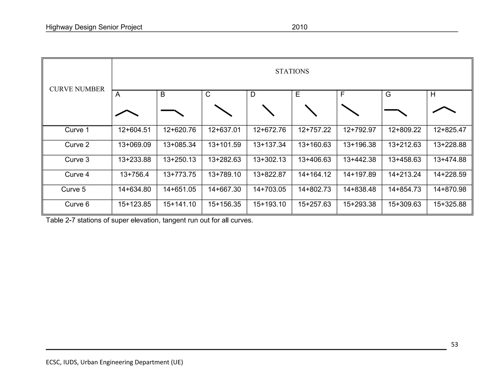
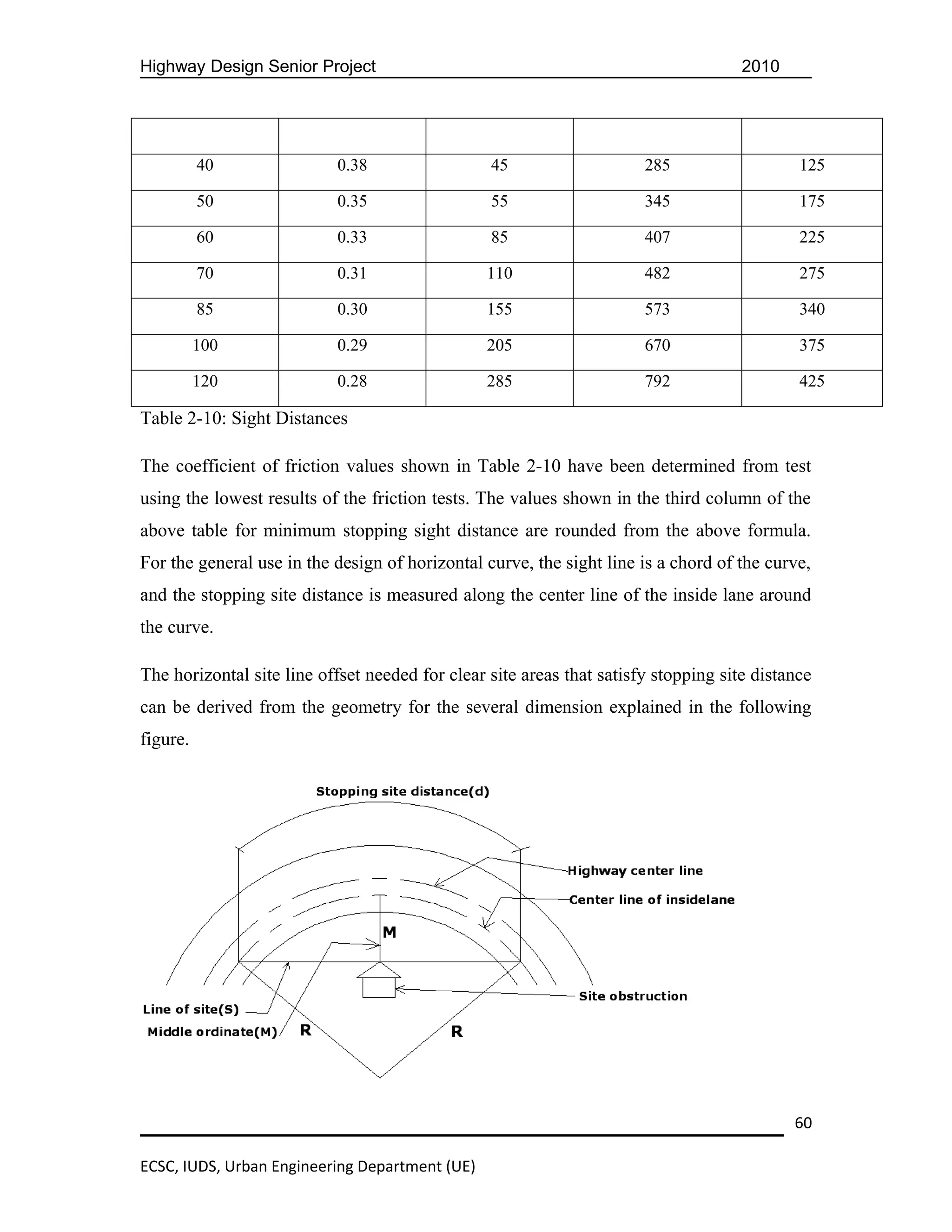
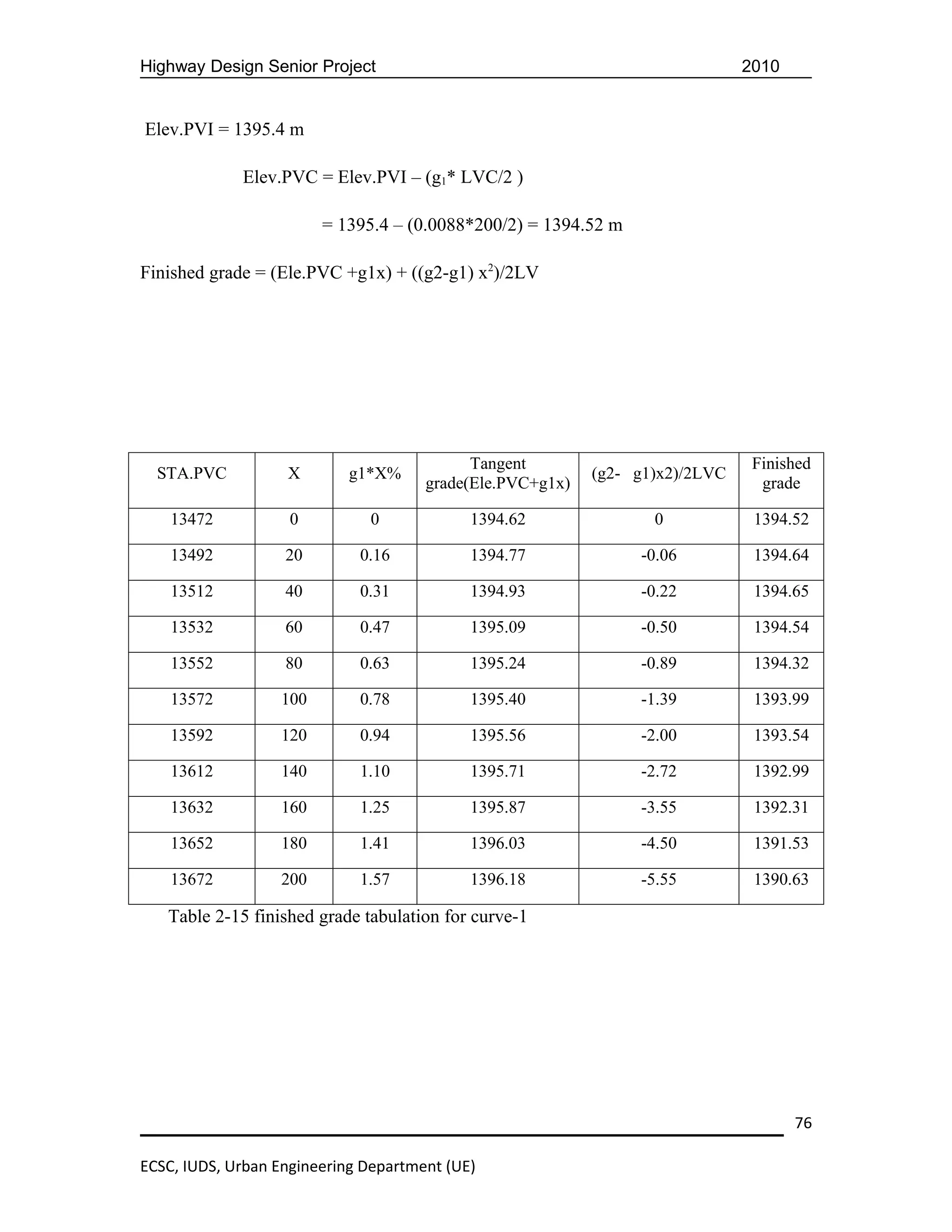
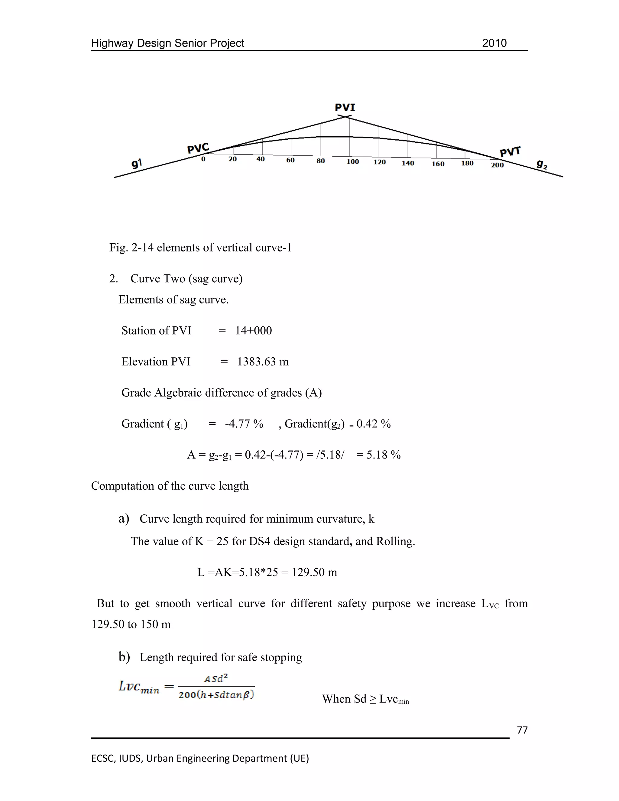
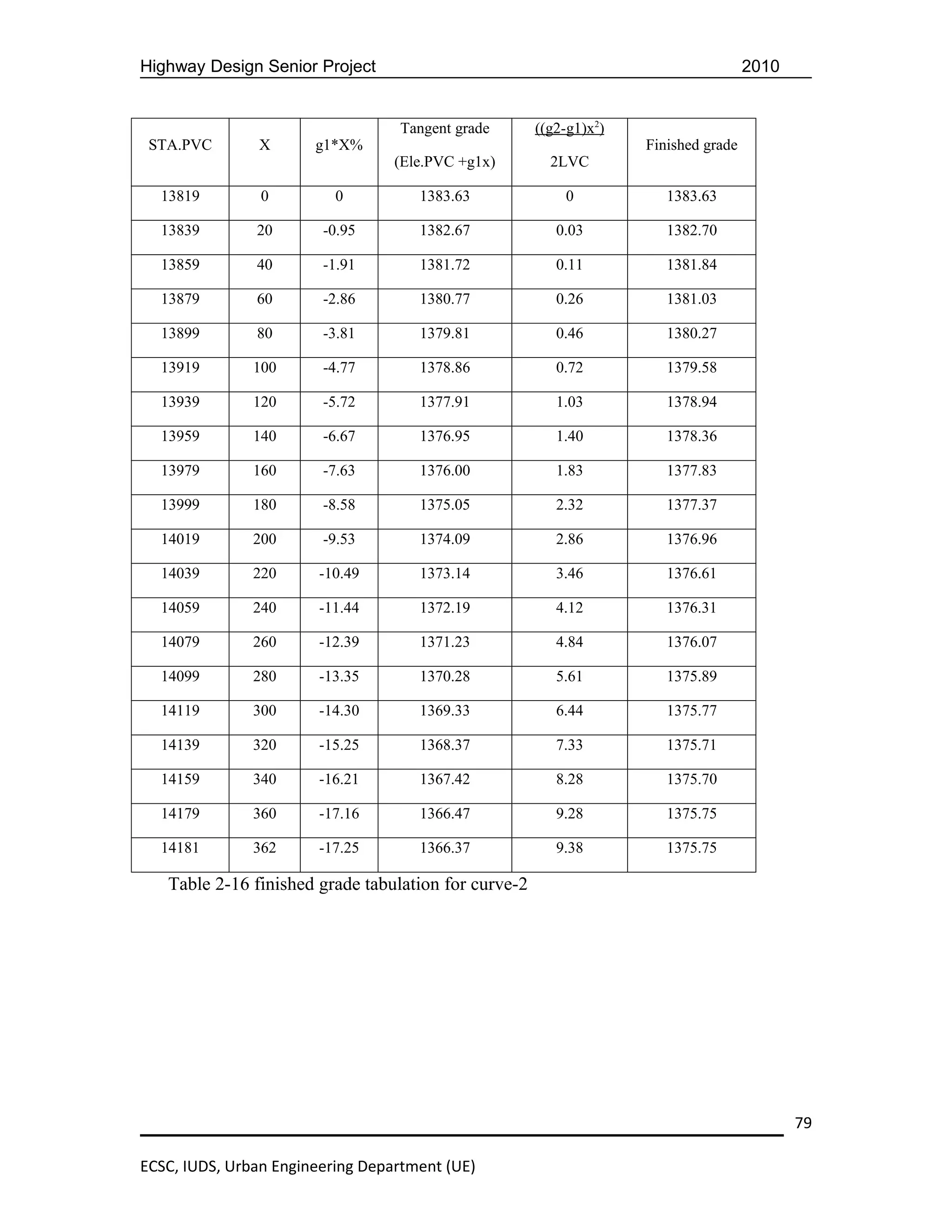
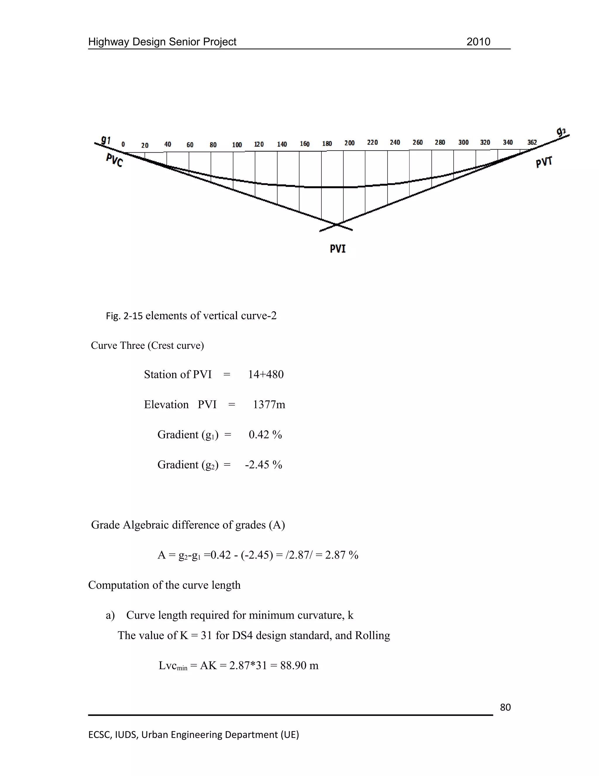
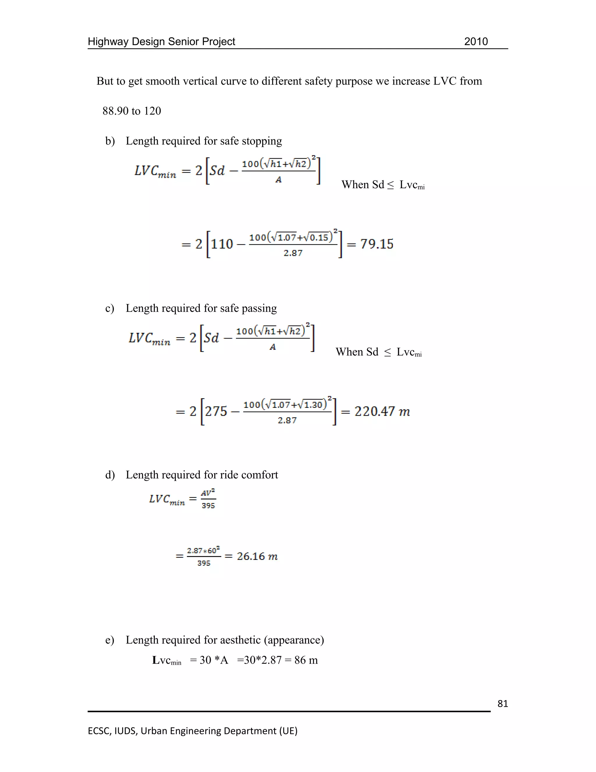
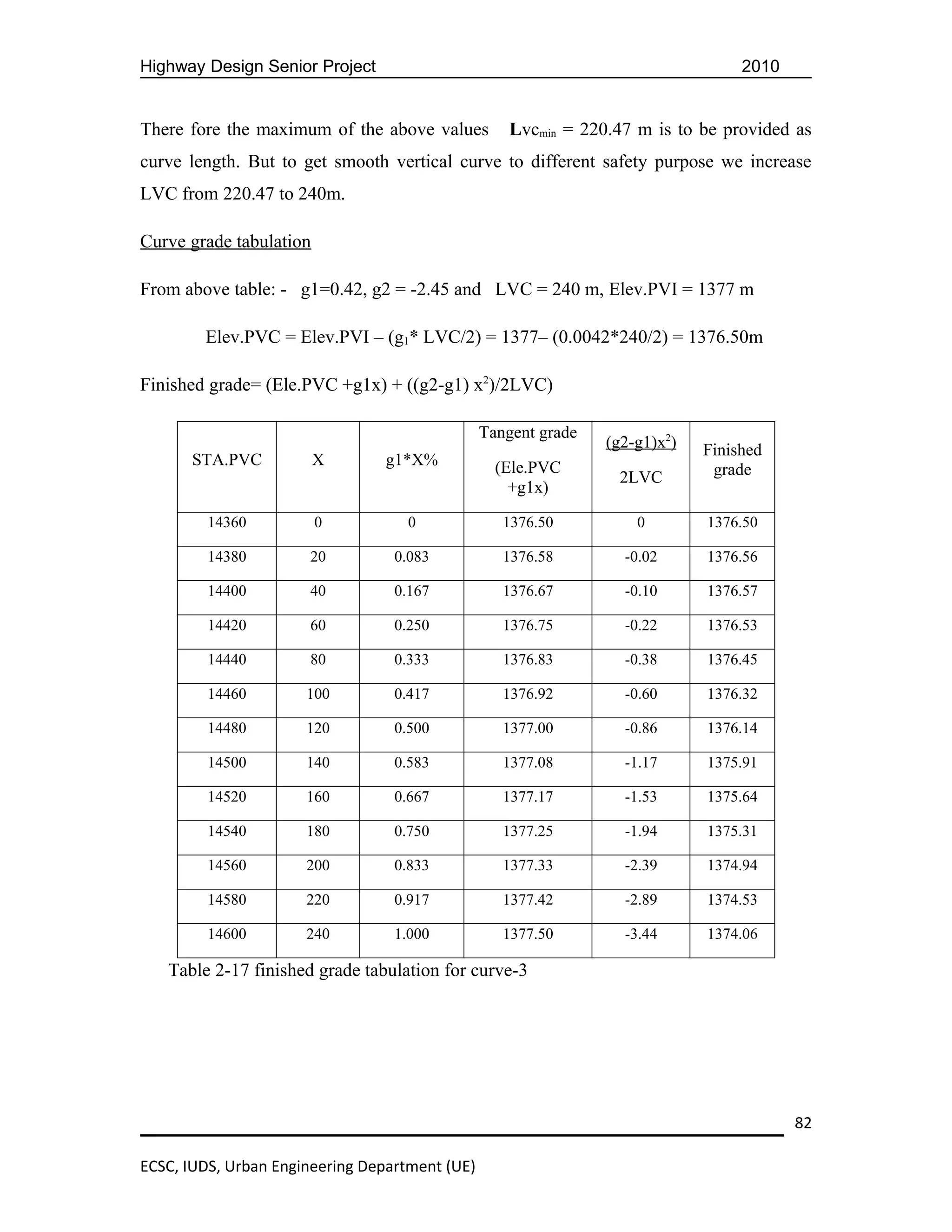
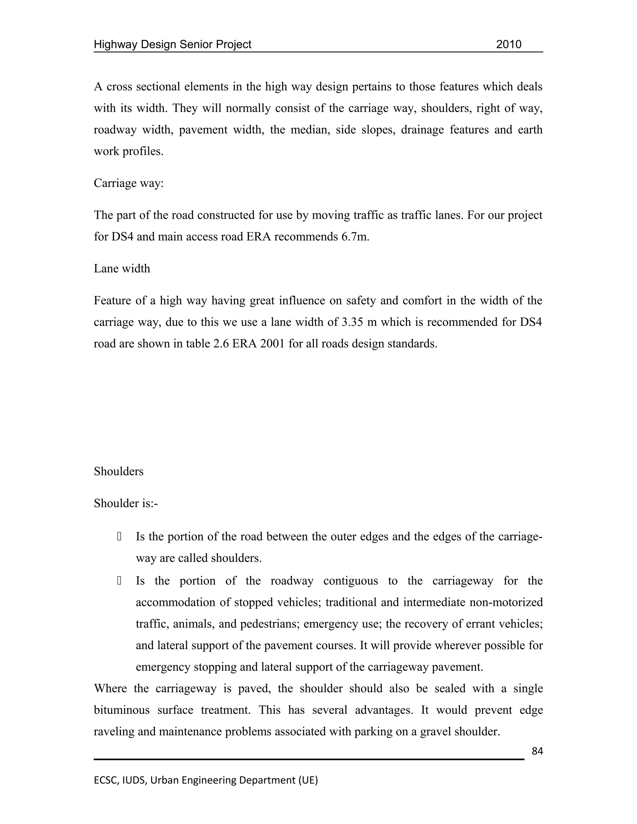
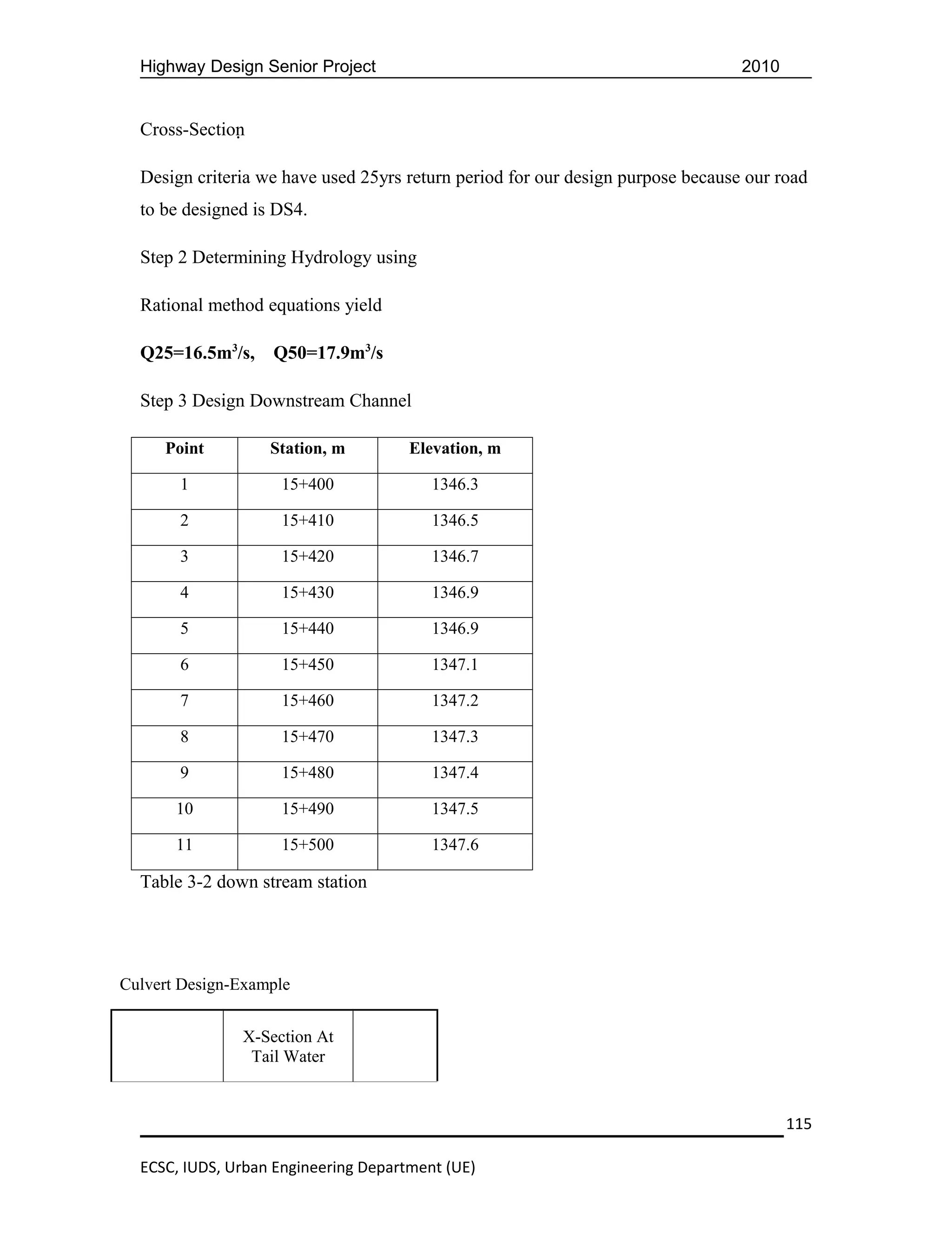
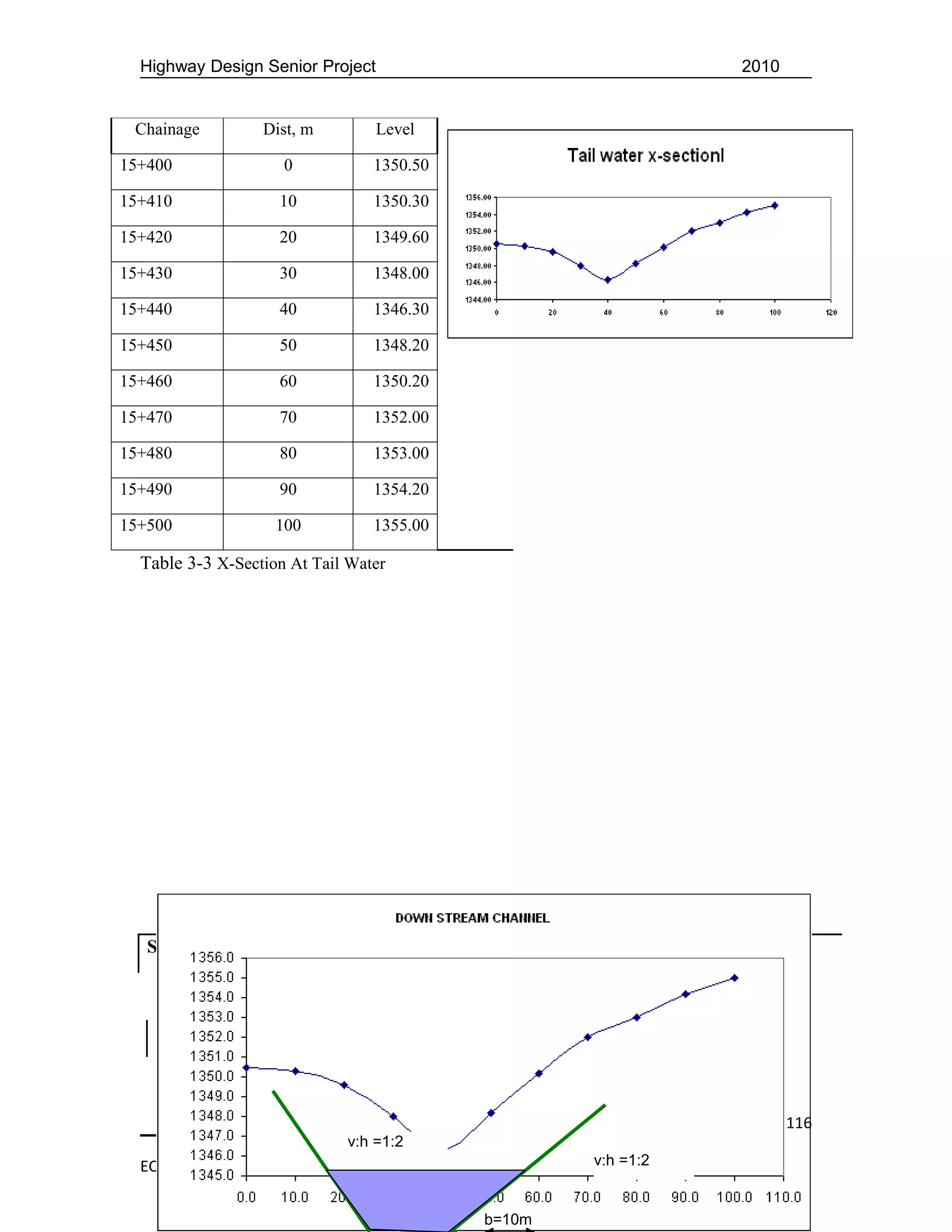
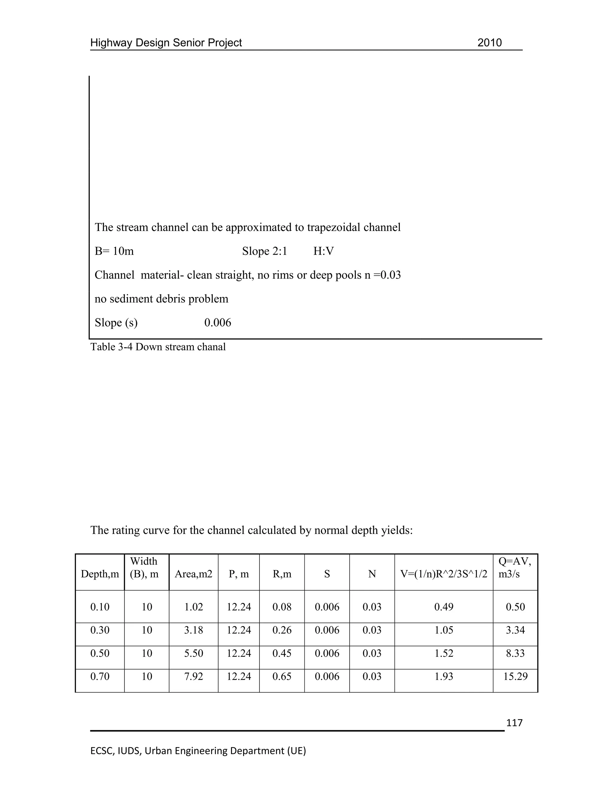
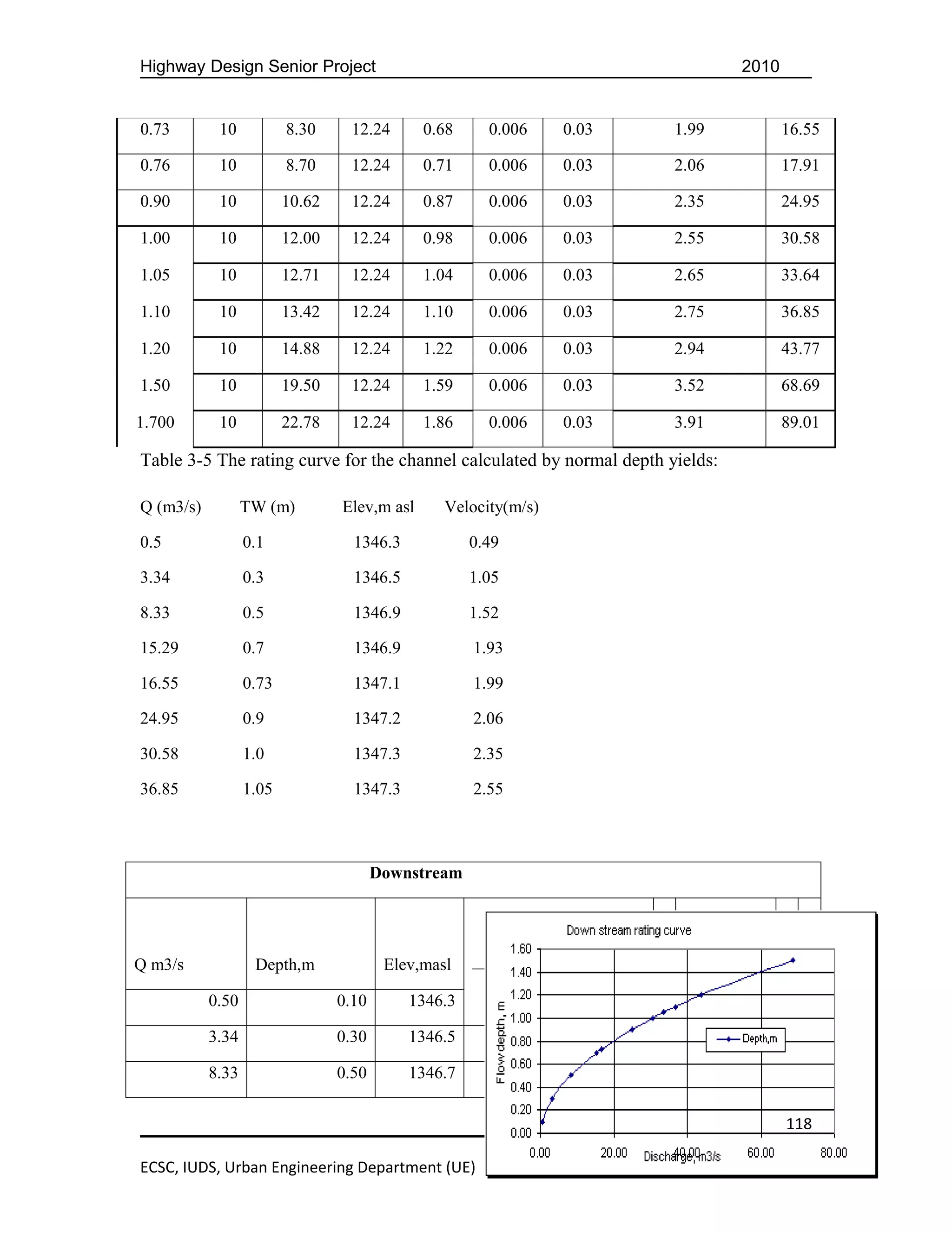
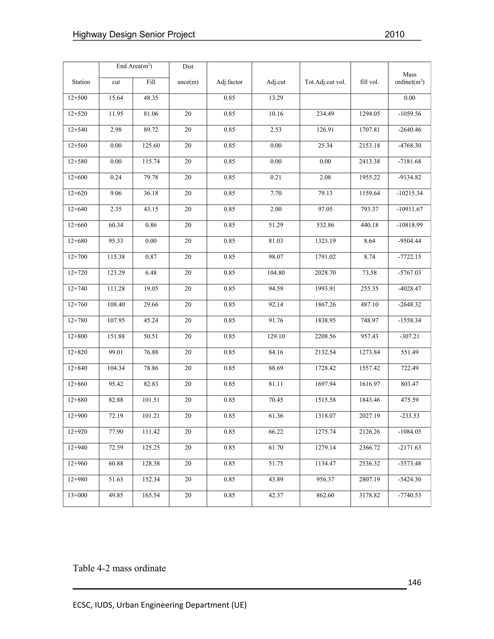
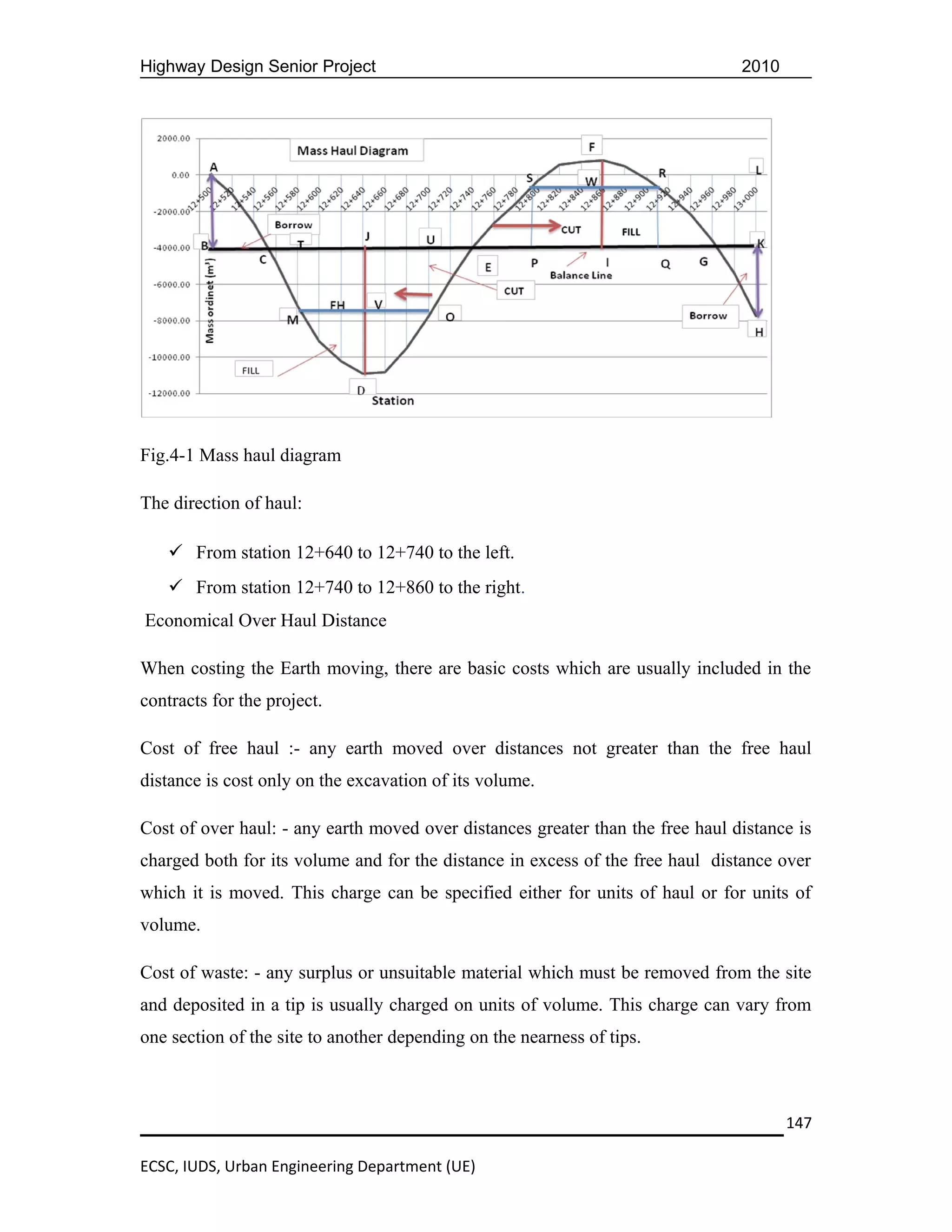
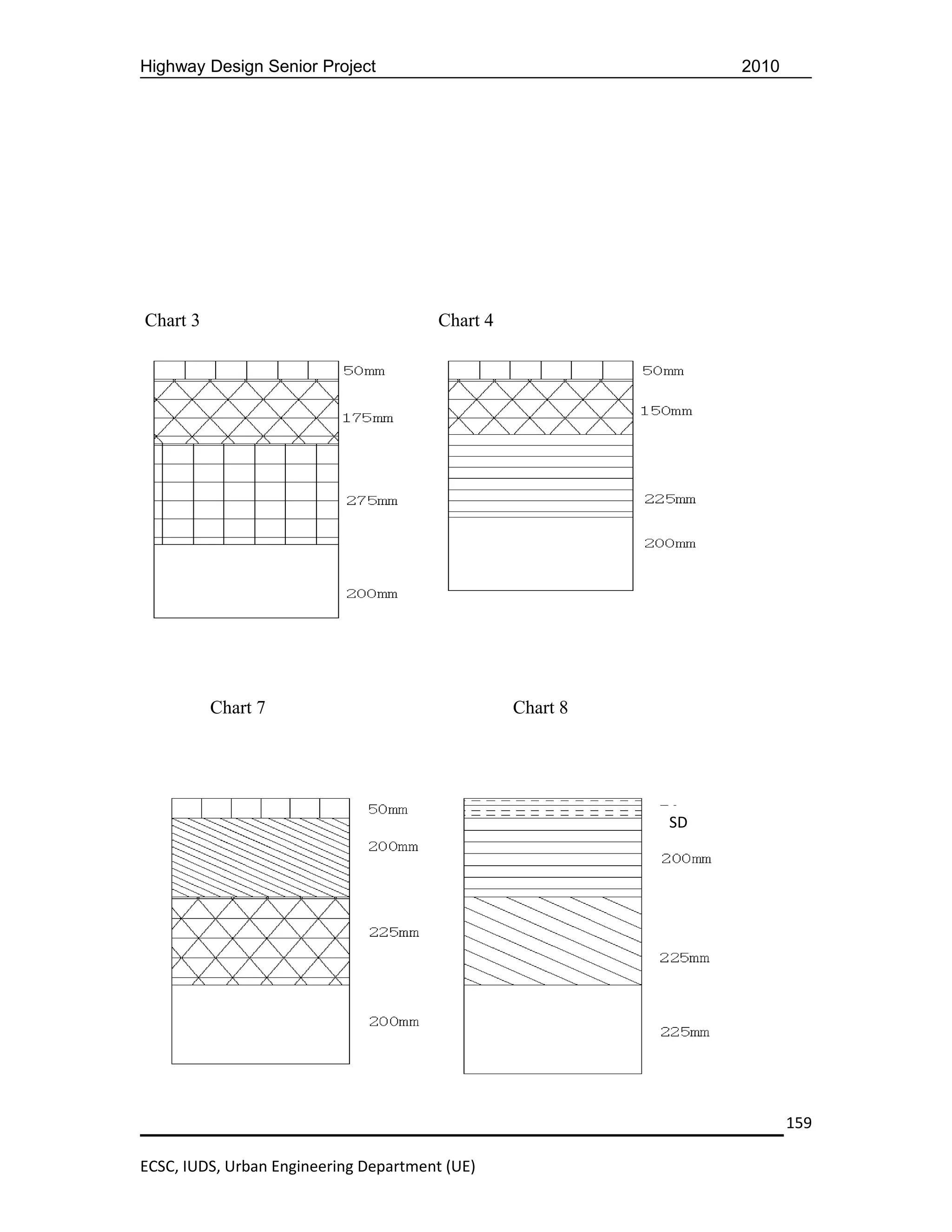
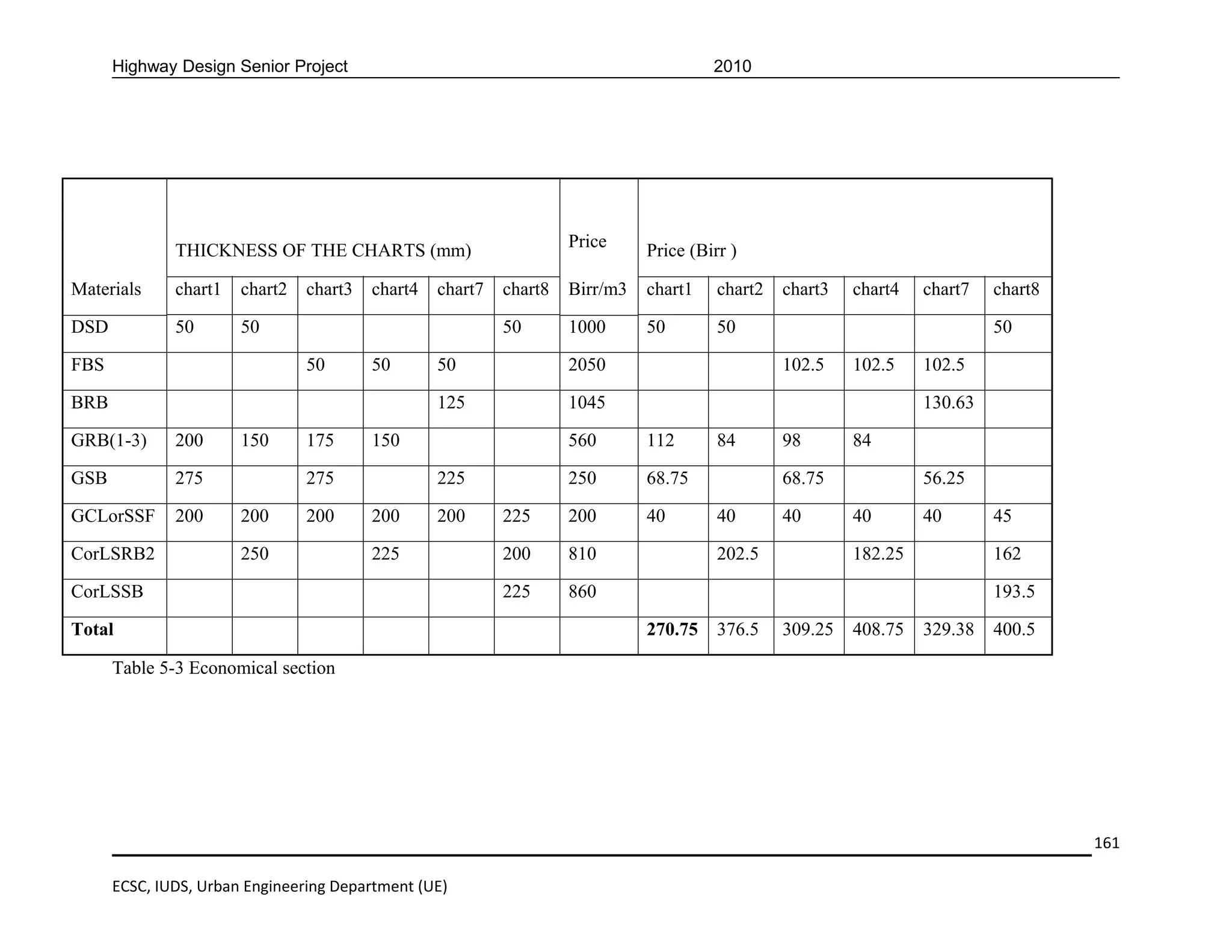
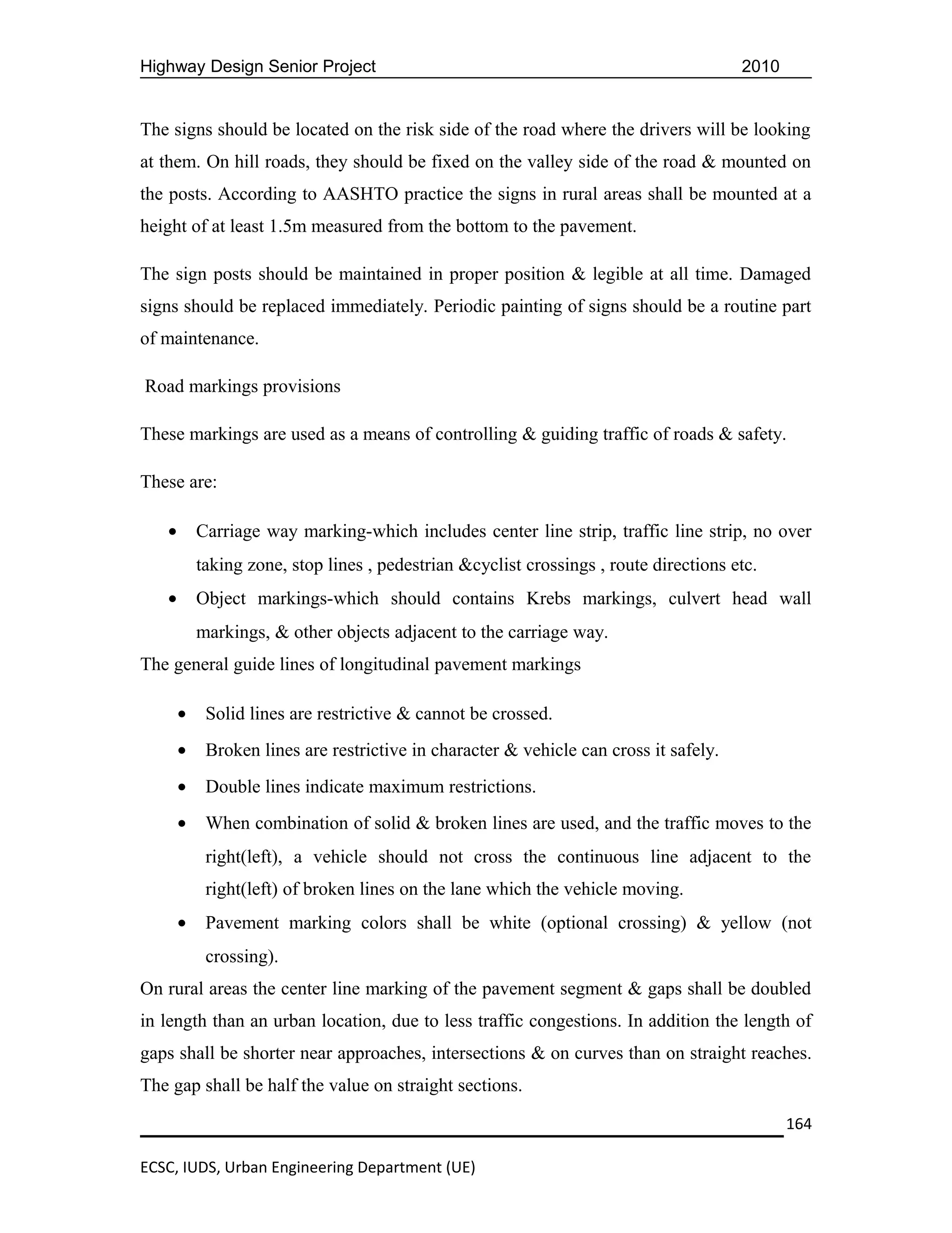
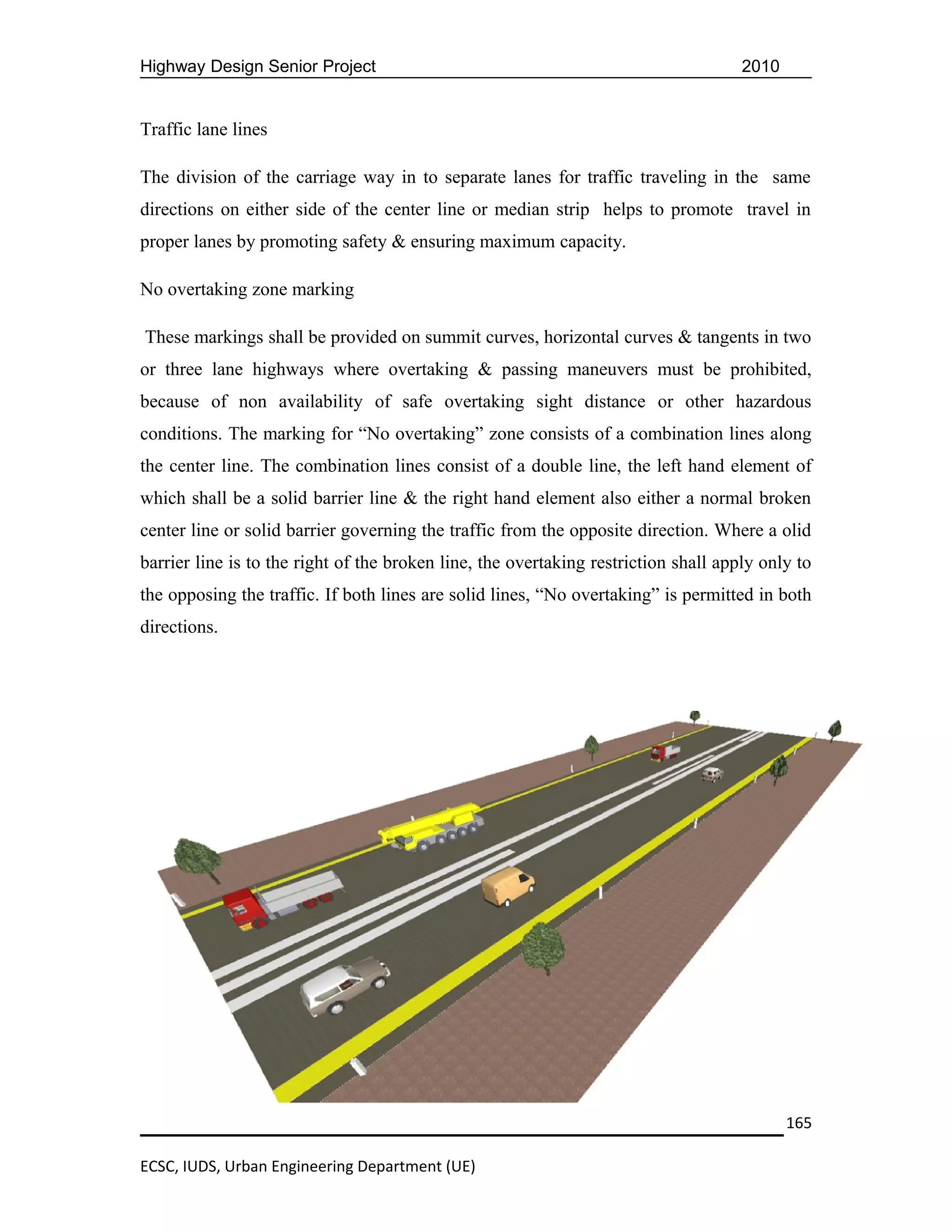
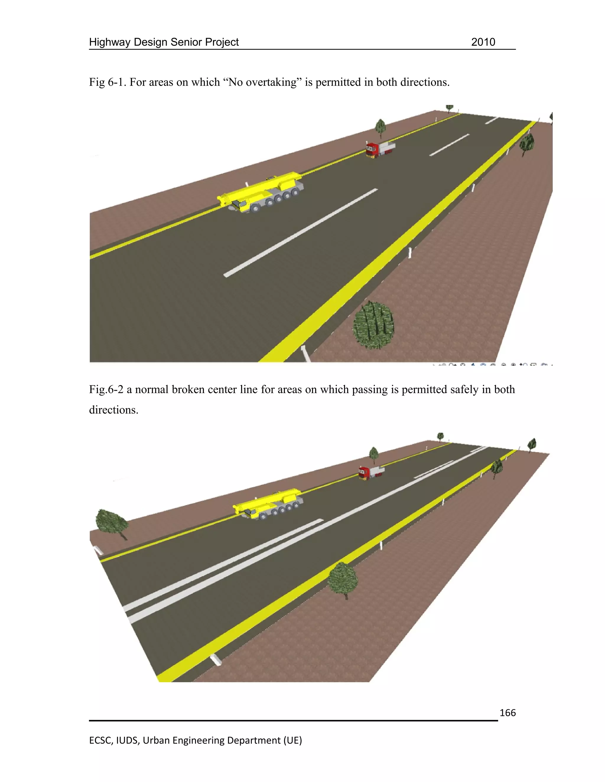
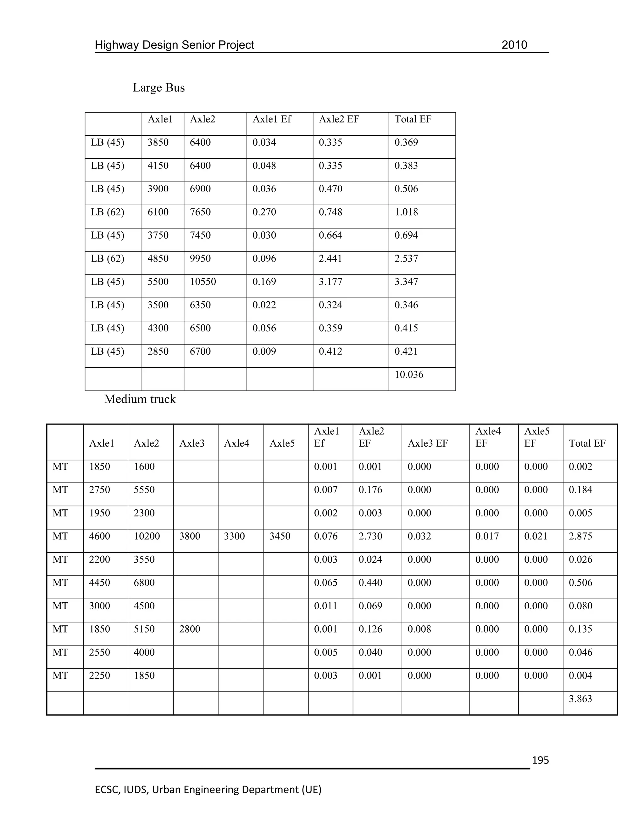
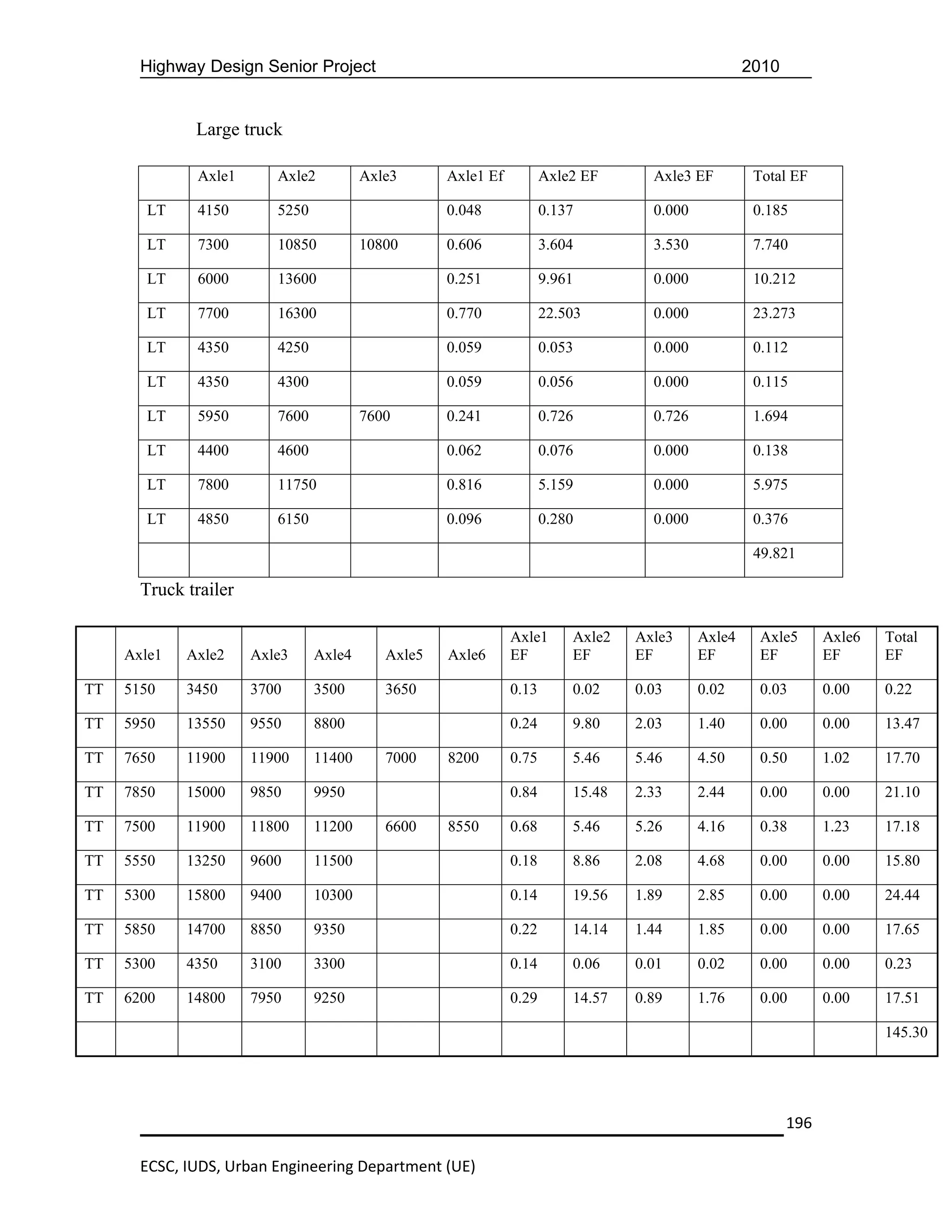
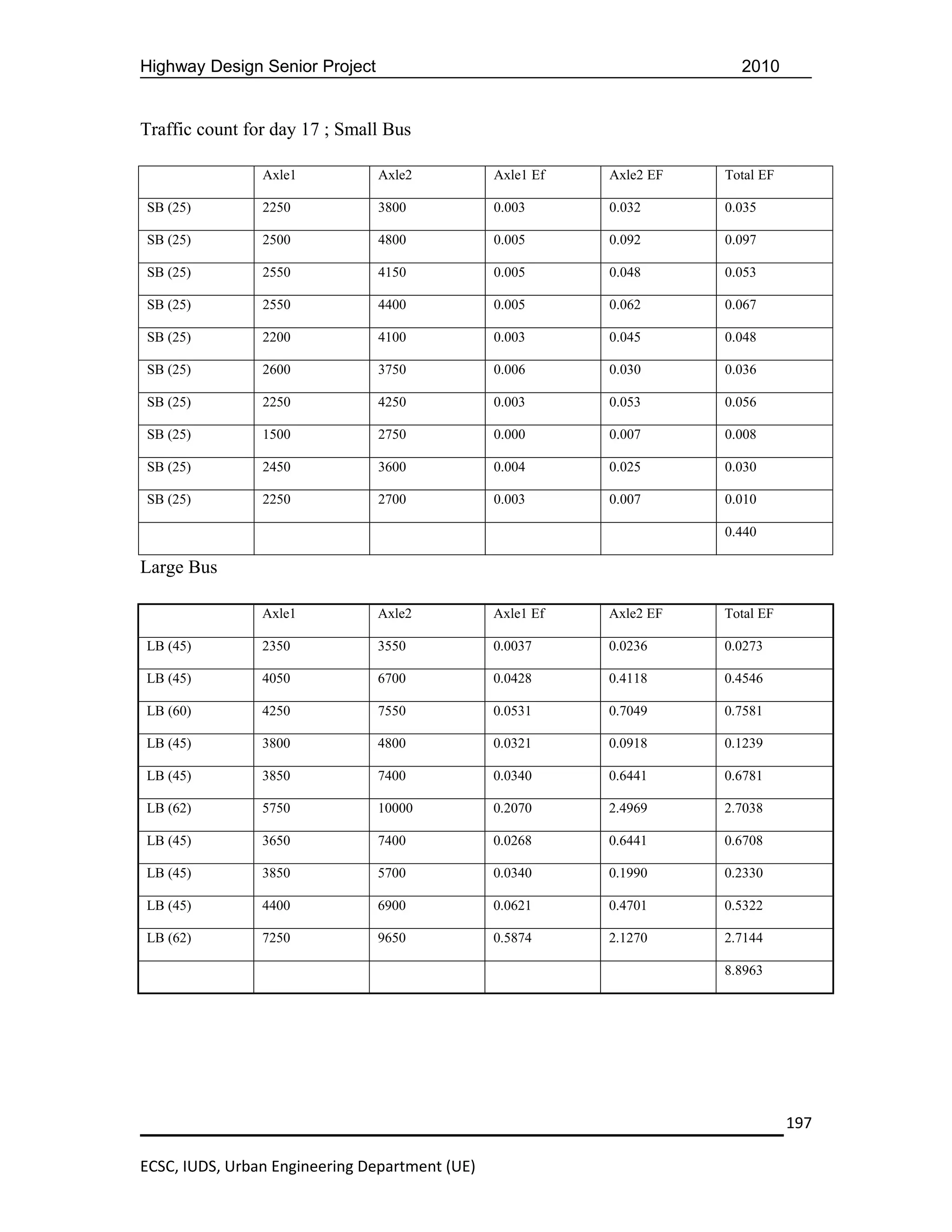
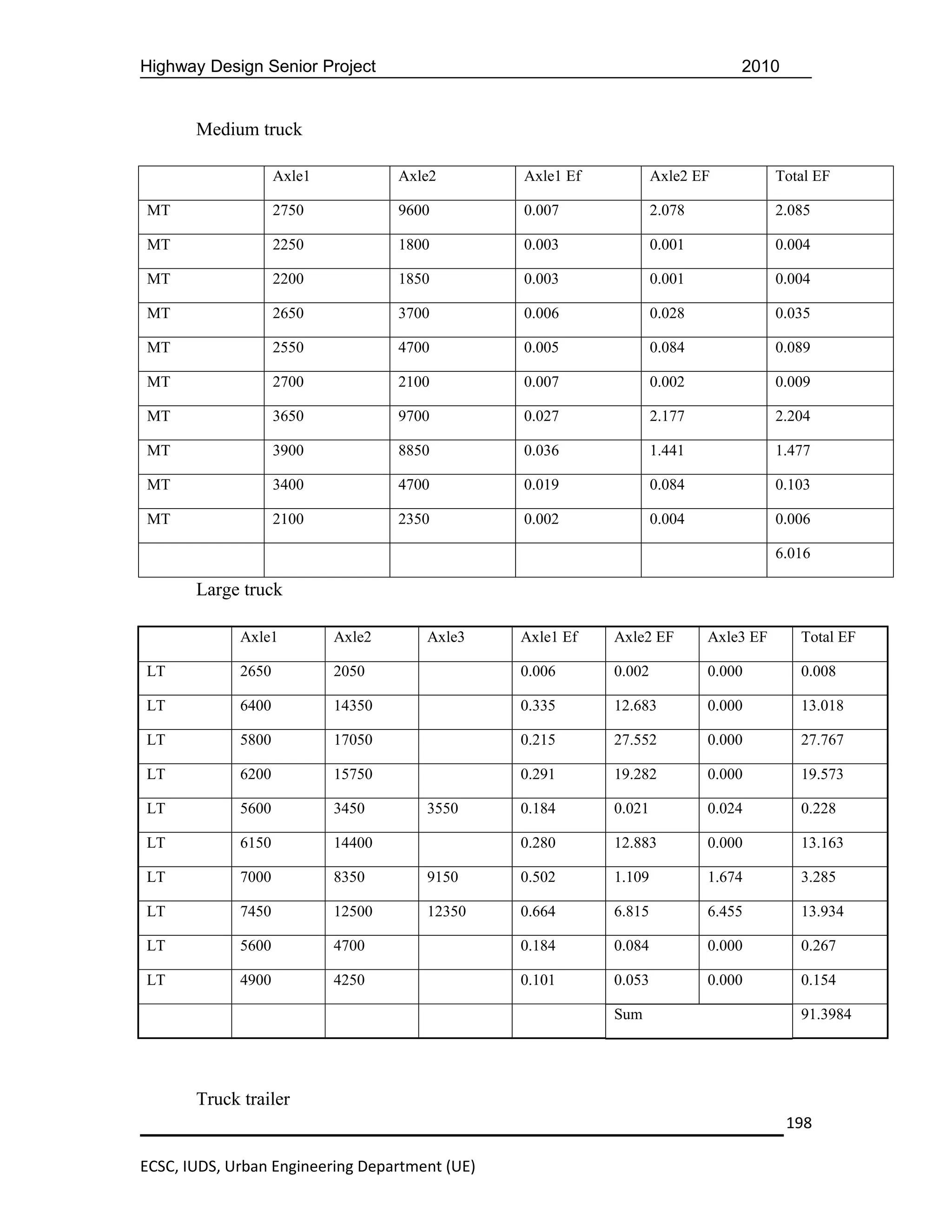
This document provides details of a highway design senior project located in eastern Ethiopia. It includes an introduction describing the need for well-trained engineers and objectives of exposing students to practical design projects. It then gives a brief description of the project area along the Hargele-Afder-Bare-Yet road and scope of the project. The next section focuses on geometric design, including terrain classification, design traffic volumes, functional classification, design standards, and computation of elements for the first horizontal curve.

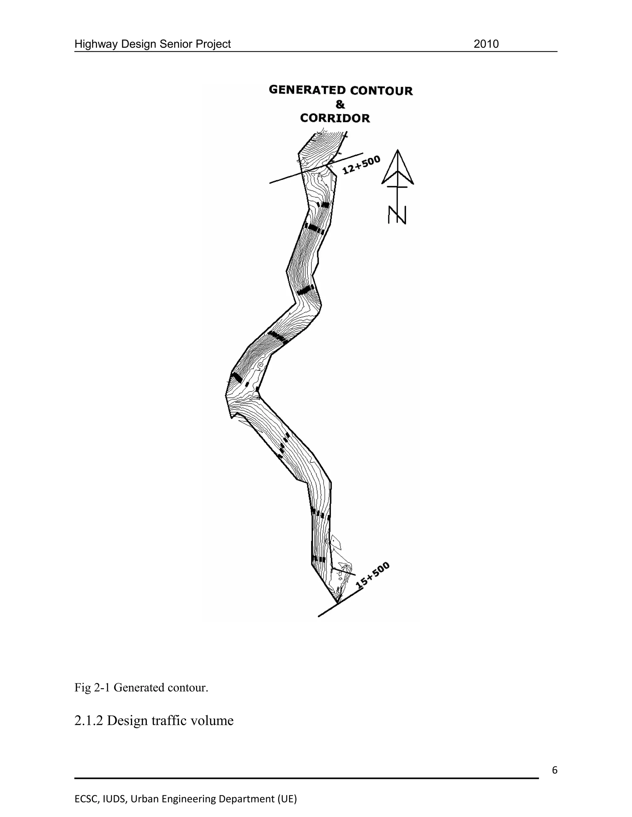


![Highway Design Senior Project 2010
V = average barrel velocity, m/s
Q = flow rate, m3/s
A = cross sectional area of flow with the barrel full, m2
Velocity Head
Hv = V2/2g where g = acceleration due to gravity, 9.8 m/s2
Entrance loss
He = Ke (V2/2g) where Ke = entrance loss coefficient,
Friction Loss
Hf = [(19.63n2L)/R1.33] [V2/2g)
Where:
n = Manning’s roughness coefficient
L = length of the culvert barrel, m
R = hydraulic radius of the full culvert barrel = A/P, m
P = wetted perimeter of the barrel, m
Exit Loss
Ho = 1.0 [(V2/2g) - (Vd2/2g)]
Where: Vd = channel velocity downstream of the culvert, m/s (usually neglected)
& Ho = Hv = V2/2g
Barrel Losses
H = He + Ho+Hf
H = [1 + Ke + (19.63n2L/R1.33)] [V2/2g]
105
ECSC, IUDS, Urban Engineering Department (UE)](https://image.slidesharecdn.com/highwaydesignraportfinalgroup2-130112062559-phpapp02/75/Highway-design-raport-final-group-2-105-2048.jpg)


![Highway Design Senior Project 2010
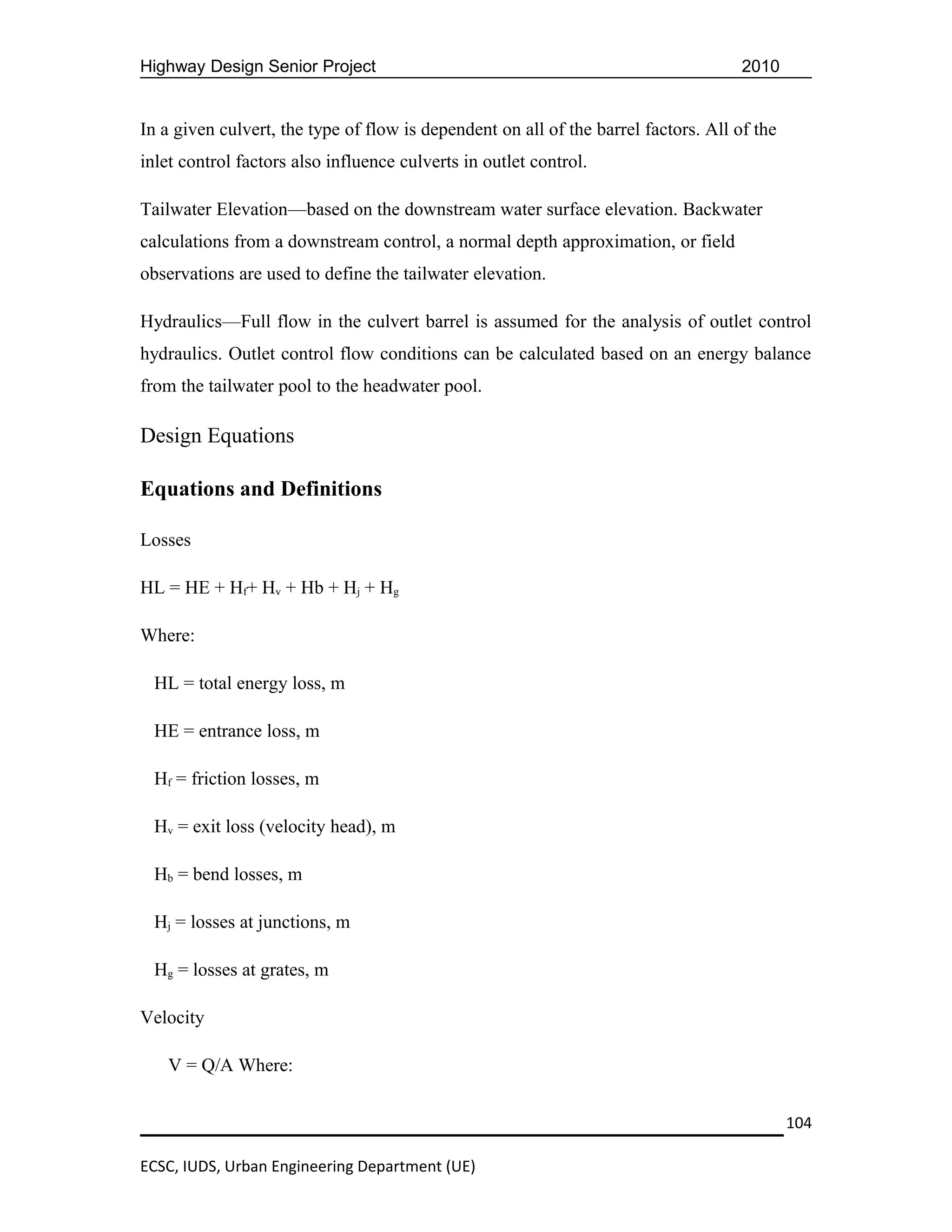
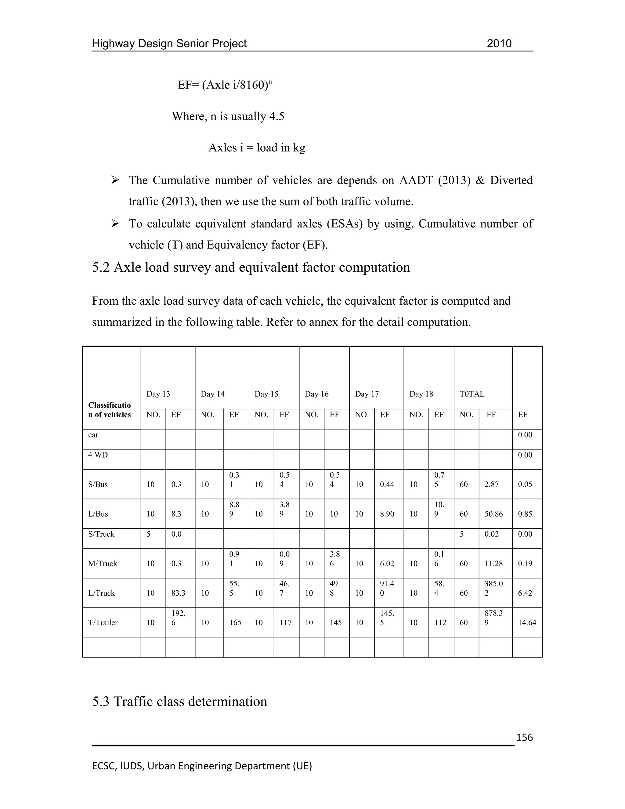
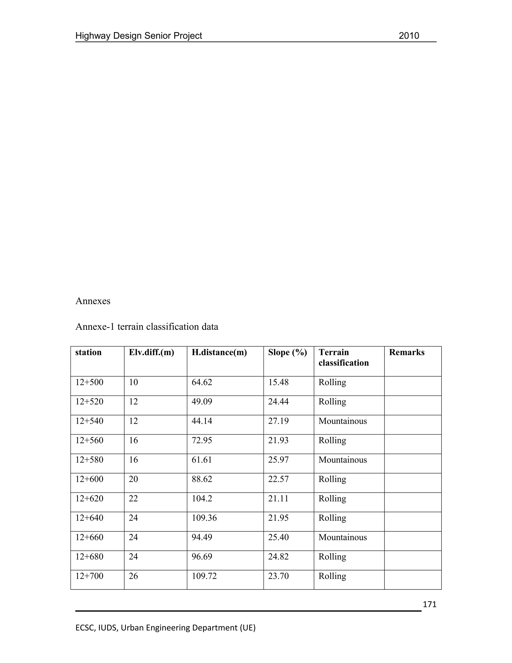
B=width of the culvert
R=A/Pw, where A=cross sectional area
R=hydraulic radius of the culvert
Pw=wetted perimeter of the clvert
Pw=B+2dn ,B=3
16.5 m3/s= (1/0.012)(3*dn)[(3*dn)/(3+2dn)]2/3(0.05)0.5
= (3*dn)[3*dn/(3+2dn)]2/3 *(0.05)0.5
=>dn=1.08m as it is shown in the following table in order to convey the total
discharge (Qt=16.5). So our trials and their corresponding results are given in the table
below.
dn 1/n A R^2/3 S^1/2 V Q
0.2 83.33 0.60 0.3 0.1 2.2 1.3
0.25 83.33 0.75 0.4 0.1 2.5 1.9
0.3 83.33 0.90 0.4 0.1 2.8 2.5
0.4 83.33 1.20 0.5 0.1 3.2 3.9
0.50 83.33 1.50 0.5 0.1 3.6 5.4
0.90 83.33 2.70 0.7 0.1 4.8 12.8
1.00 83.33 3.00 0.7 0.1 5.0 14.9
1.05 83.33 3.15 0.7 0.1 5.1 15.9
1.08 83.33 3.24 0.7 0.1 5.1 16.6
1.10 83.33 3.30 0.7 0.1 5.1 17.0
1.15 83.33 3.45 0.8 0.1 5.2 18.1
122
ECSC, IUDS, Urban Engineering Department (UE)](https://image.slidesharecdn.com/highwaydesignraportfinalgroup2-130112062559-phpapp02/75/Highway-design-raport-final-group-2-122-2048.jpg)

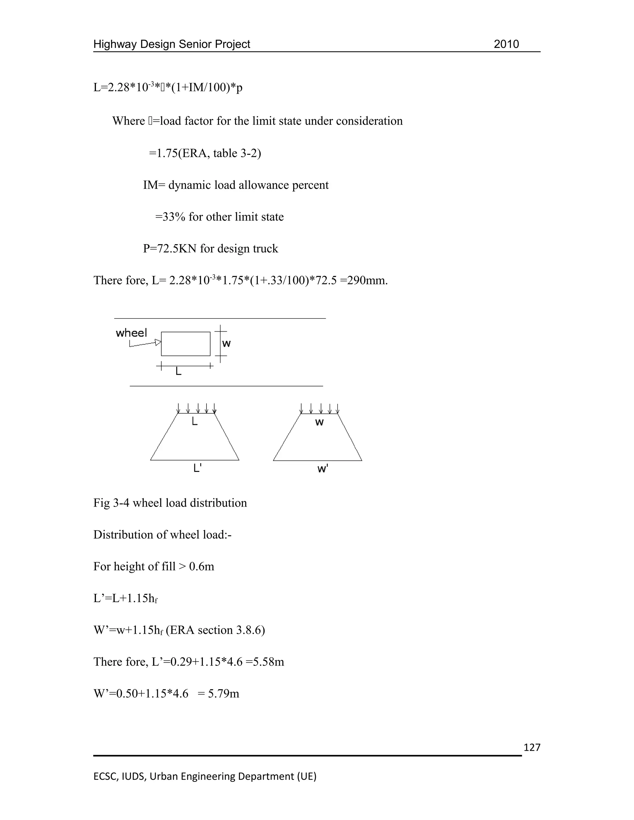
![Highway Design Senior Project 2010
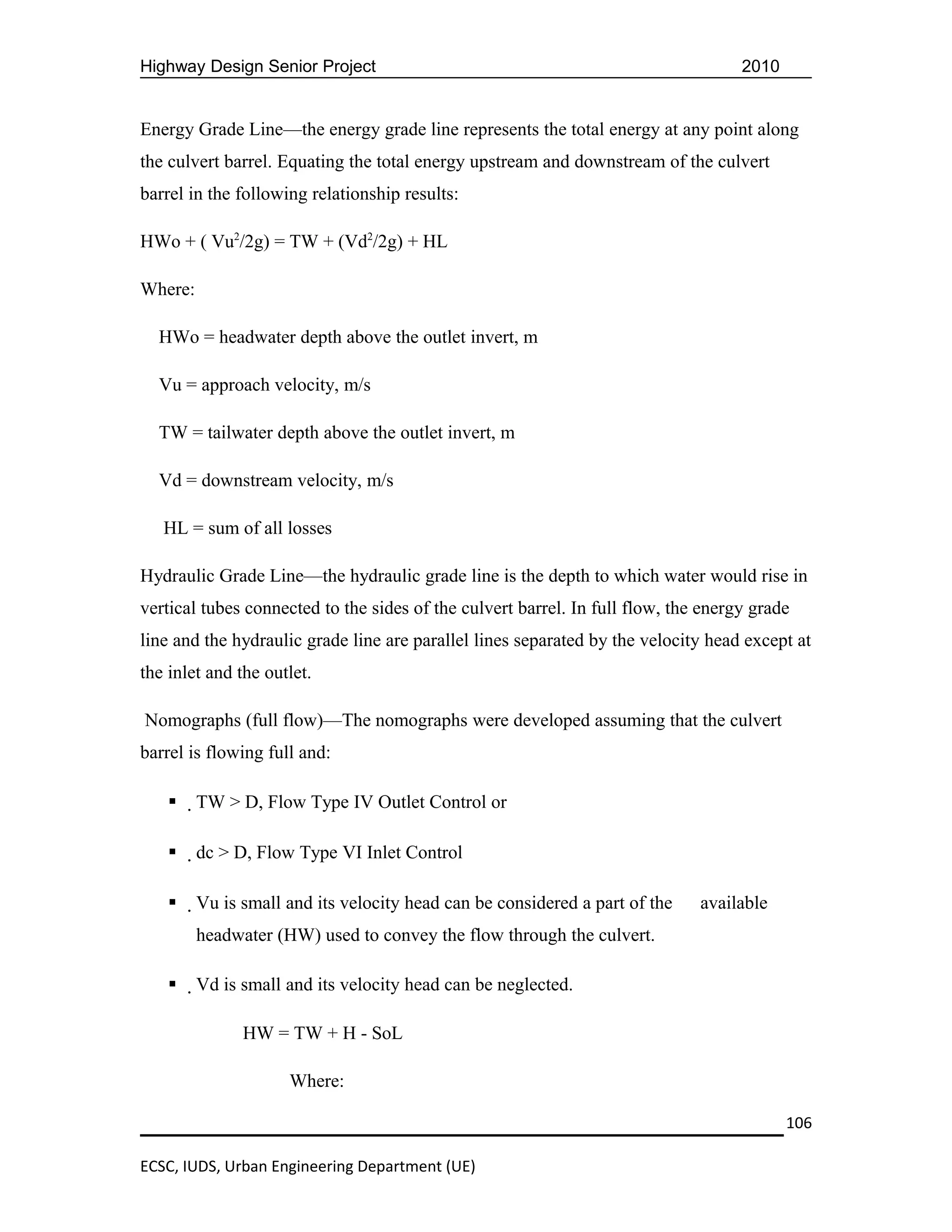
But L’ is greater than the span of the culvert. There fore the intensity of the live loading
needs to be reduced proportionally.
Reduced load= (72.5*3.6)/5.58 =46.77KN
Load with impact factor=1.25*46.77 =58.47KN
Intensity of live load on the slab:
Intensity=load/area
=load/ (culvert span*w’)
=58.47/ (3.6*5.79)=2.805KN/m2 =2805N/m2
3/ Load and reaction calculation
Dead load of the top slab:-
=0.3*1*25000=7500N/m2=75KN/m2
Total load on the culvert=Dead load +Live load
=82.8KN/m2+2.805kN/m2=85.605KN/m2=85605N/2
There fore,
Total design load on the top slab=85605N/2+7,500N/m2
=93,105N/m2
Weight of each wall (side wall) =2.3*0.3*25000=17,250N/m
Then, up ward reaction at the base
= [(93,105*3.3) + (2*17250)]/3.3*1
=103,559N/m2
128
ECSC, IUDS, Urban Engineering Department (UE)](https://image.slidesharecdn.com/highwaydesignraportfinalgroup2-130112062559-phpapp02/75/Highway-design-raport-final-group-2-128-2048.jpg)
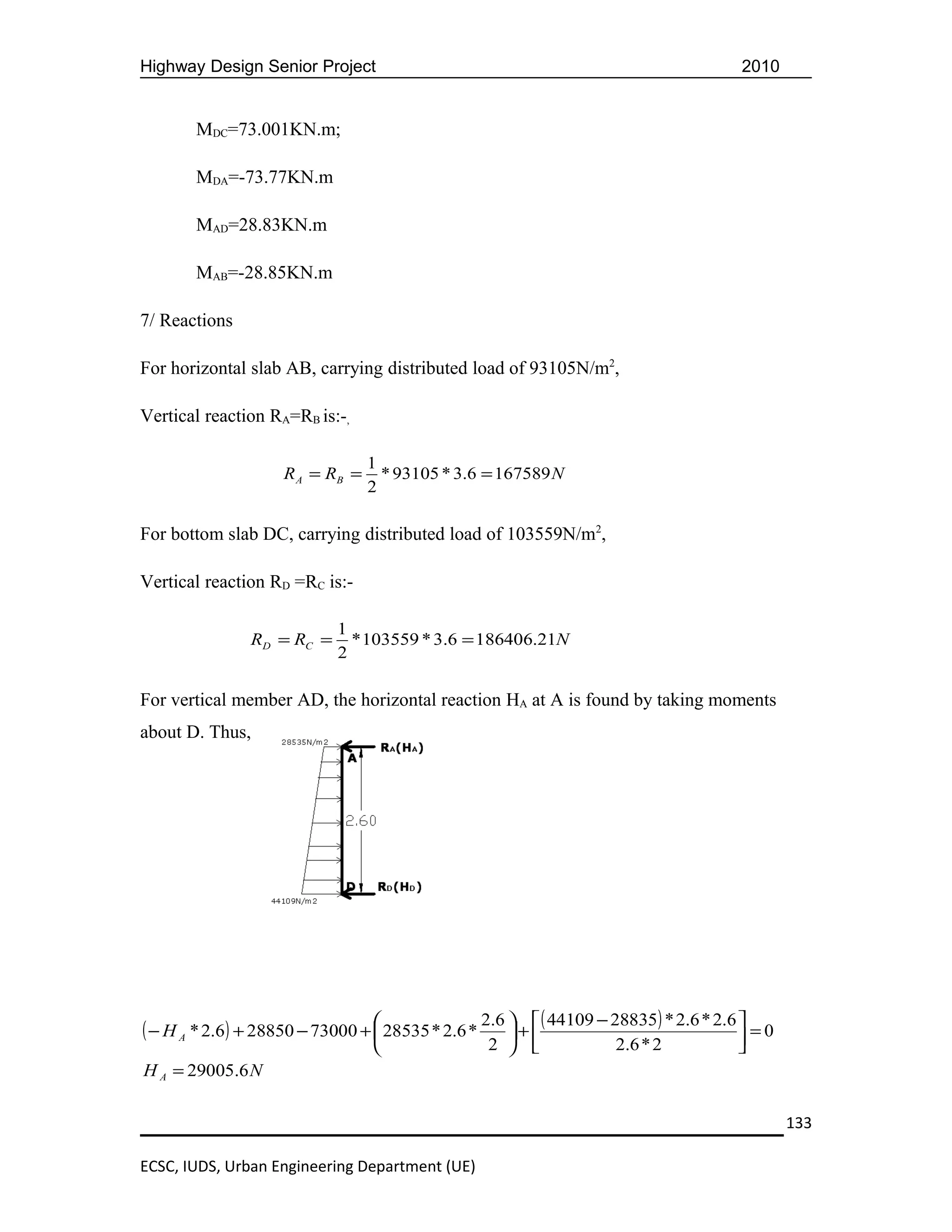


![[PDF]PROJECT ON HIGHWAY BY SUBHENDU SAMUI](https://cdn.slidesharecdn.com/ss_thumbnails/project-report-subhendu-160225031340-thumbnail.jpg?width=640&height=640&fit=bounds)


