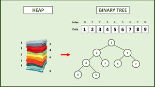
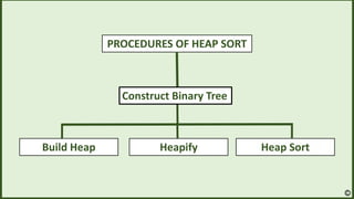
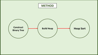
The document provides a detailed explanation of the heap sort algorithm, including its history, definitions, and the steps involved in executing the algorithm. It outlines key concepts like building a max heap, the procedure of heapifying an array, and implementing the sort through pseudocode. The content is structured academically for a computer science course, making it suitable for students learning sorting algorithms.

1. TOPIC: HEAP SORT
Group: 12
Date: 13/09/2022
COURSE : CSE 2218/CSI 228 (C)
Faculty:
Sufi Aurangzeb Hossain
LECTURER (ADJUNCT)
DEPT. OF COMPUTER SCIENCE & ENGINEERING
011201230 Santi Brata Nath Joy
011201295 Md. Tanzid Ahsan
MEMBERS
011201214 Saikat Hossain

2. HISTORY
Sir John William Joseph Williams
1964 Instant Access

3. DEFINATION
Sorting Algorithm
Binary Tree Heap
O (N log N)

4. HEAP BINARY TREE
1
3
2
4
6
5
7
8
1
2 3
4 5
9
6 7
8 9
5
Index
Data 6 7 8 9
5 6 7 8
3
2 4
1
0 1 2 3 4

5. HEAP PROPERTY
Max Heap Min Heap
10
5 3
4 1
1
3 5
4 7
A[Parent(i)] ≥ A[i] A[Parent(i)] ≤ A[i]
3
5 4 1
10
0 1 2 3 4
Index
Data 5
3 4 7
1
0 1 2 3 4

6. PROCEDURES OF HEAP SORT
Heapify Heap Sort
Build Heap
Construct Binary Tree

7. HEAPIFY
Heapify(A, i)
{
l <- left(i)
r <- right(i)
if l <= heapsize[A] and A[l] > A[i]
then largest <- l
else largest <- i
if r <= heapsize[A] and A[r] > A[largest]
then largest <- r
if largest != i
then swap A[i] <-A[largest]
Heapify(A, largest)
}
4
10 3
10
4 3
Swap

8. BUILD HEAP
3
10 5 1
4
0 1 2 3 4
Index
Data
4
10 3
5 1
Internal Nodes
Buildheap(A)
{
heapsize[A] length[A]
for i |length[A]/2 //down to 0
do Heapify(A, i)
}

9. BUILD HEAP
Buildheap(A)
{
heapsize[A] length[A]
for i |length[A]/2 //down to 0
do Heapify(A, i)
}
3
5 4 1
10
0 1 2 3 4
Index
Data
10
5 3
4 1

10. HEAP SORT
Heapsort(A)
{
Buildheap(A)
for i  length[A]
do swap A[1]  A[i]
heapsize[A]  heapsize[A] - 1
Heapify(A, 1)
}
0 1 2 3 4
4
3 5 10
1
Index
Data
3
5 4 1
10
0 1 2 3 4
Index
Data
0 1 2 3 4
3
5 4 1
10
Index
Data
Swap
0 1 2 3 4
3
5 4 10
1
Index
Data

11. METHOD
Heap Sort
Construct
Binary Tree
Build Heap

12. SIMULATION
PARENT (i)
return floor(i/2)
LEFT (i)
return 2i
RIGHT (i)
return 2i + 1
3
10 5 1
4
0 1 2 3 4
Index
Data

13. SIMULATION
3
10 5 1
4
0 1 2 3 4
Index
Data
4
PARENT (i)
return floor(i/2)
LEFT (i)
return 2i
RIGHT (i)
return 2i + 1

14. SIMULATION
3
10 5 1
4
0 1 2 3 4
Index
Data
4
10
PARENT (i)
return floor(i/2)
LEFT (i)
return 2i
RIGHT (i)
return 2i + 1

15. SIMULATION
3
10 5 1
4
0 1 2 3 4
Index
Data
4
10 3
PARENT (i)
return floor(i/2)
LEFT (i)
return 2i
RIGHT (i)
return 2i + 1

16. SIMULATION
3
10 5 1
4
0 1 2 3 4
Index
Data
4
10 3
5
PARENT (i)
return floor(i/2)
LEFT (i)
return 2i
RIGHT (i)
return 2i + 1

17. SIMULATION
3
10 5 1
4
0 1 2 3 4
Index
Data
4
10 3
5 1
Done
PARENT (i)
return floor(i/2)
LEFT (i)
return 2i
RIGHT (i)
return 2i + 1

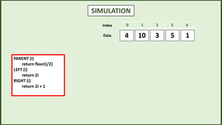
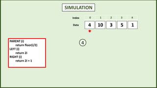
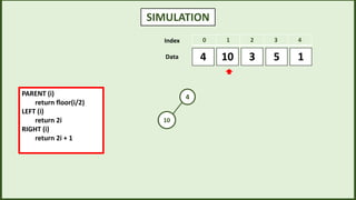
18. SIMULATION
3
10 5 1
4
0 1 2 3 4
Index
Data
4
10 3
5 1
Heapify(A, i)
{
l <- left(i)
r <- right(i)
if l <= heapsize[A] and A[l] > A[i]
then largest <- l
else largest <- i
if r <= heapsize[A] and A[r] > A[largest]
then largest <- r
if largest != i
then swap A[i] <-A[largest]
Heapify(A, largest)
}
Buildheap(A)
{
heapsize[A] length[A]
for i |length[A]/2
do Heapify(A, i)
}
Heapsort(A)
{
Buildheap(A)
for i  length[A]
do swap A[1]  A[i]
heapsize[A]  heapsize[A] - 1
Heapify(A, 1)
}

19. SIMULATION
3
10 5 1
4
0 1 2 3 4
Index
Data
4
10 3
5 1
10 is greater than 4
then swap A[i] <-A[largest]
Swap 4 and 10
Swap
Heapify(A, i)
{
l <- left(i)
r <- right(i)
if l <= heapsize[A] and A[l] > A[i]
then largest <- l
else largest <- i
if r <= heapsize[A] and A[r] > A[largest]
then largest <- r
if largest != i
then swap A[i] <-A[largest]
Heapify(A, largest)
}
Buildheap(A)
{
heapsize[A] length[A]
for i |length[A]/2
do Heapify(A, i)
}
Heapsort(A)
{
Buildheap(A)
for i  length[A]
do swap A[1]  A[i]
heapsize[A]  heapsize[A] - 1
Heapify(A, 1)
}

20. SIMULATION
3
4 5 1
10
0 1 2 3 4
Index
Data
10
4 3
5 1
Heapify(A, i)
{
l <- left(i)
r <- right(i)
if l <= heapsize[A] and A[l] > A[i]
then largest <- l
else largest <- i
if r <= heapsize[A] and A[r] > A[largest]
then largest <- r
if largest != i
then swap A[i] <-A[largest]
Heapify(A, largest)
}
Buildheap(A)
{
heapsize[A] length[A]
for i |length[A]/2
do Heapify(A, i)
}
Heapsort(A)
{
Buildheap(A)
for i  length[A]
do swap A[1]  A[i]
heapsize[A]  heapsize[A] - 1
Heapify(A, 1)
}

21. SIMULATION
3
4 5 1
10
0 1 2 3 4
Index
Data
5 is greater than 4
then swap A[i] <-A[largest]
Swap 5 and 4
10
4 3
5 1
Swap
Heapify(A, i)
{
l <- left(i)
r <- right(i)
if l <= heapsize[A] and A[l] > A[i]
then largest <- l
else largest <- i
if r <= heapsize[A] and A[r] > A[largest]
then largest <- r
if largest != i
then swap A[i] <-A[largest]
Heapify(A, largest)
}
Buildheap(A)
{
heapsize[A] length[A]
for i |length[A]/2
do Heapify(A, i)
}
Heapsort(A)
{
Buildheap(A)
for i  length[A]
do swap A[1]  A[i]
heapsize[A]  heapsize[A] - 1
Heapify(A, 1)
}

22. SIMULATION
3
5 4 1
10
0 1 2 3 4
Index
Data
10
5 3
4 1
Heapify(A, i)
{
l <- left(i)
r <- right(i)
if l <= heapsize[A] and A[l] > A[i]
then largest <- l
else largest <- i
if r <= heapsize[A] and A[r] > A[largest]
then largest <- r
if largest != i
then swap A[i] <-A[largest]
Heapify(A, largest)
}
Buildheap(A)
{
heapsize[A] length[A]
for i |length[A]/2
do Heapify(A, i)
}
Heapsort(A)
{
Buildheap(A)
for i  length[A]
do swap A[1]  A[i]
heapsize[A]  heapsize[A] - 1
Heapify(A, 1)
}

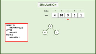
23. SIMULATION
3
5 4 1
10
0 1 2 3 4
Index
Data
10
5 3
4 1
After Build Heap
Heapify(A, i)
{
l <- left(i)
r <- right(i)
if l <= heapsize[A] and A[l] > A[i]
then largest <- l
else largest <- i
if r <= heapsize[A] and A[r] > A[largest]
then largest <- r
if largest != i
then swap A[i] <-A[largest]
Heapify(A, largest)
}
Buildheap(A)
{
heapsize[A] length[A]
for i |length[A]/2
do Heapify(A, i)
}
Heapsort(A)
{
Buildheap(A)
for i  length[A]
do swap A[1]  A[i]
heapsize[A]  heapsize[A] - 1
Heapify(A, 1)
}

24. SIMULATION
0 1 2 3 4
3
5 4 1
10
Index
Data
10
5 3
4 1
Heapify(A, i)
{
l <- left(i)
r <- right(i)
if l <= heapsize[A] and A[l] > A[i]
then largest <- l
else largest <- i
if r <= heapsize[A] and A[r] > A[largest]
then largest <- r
if largest != i
then swap A[i] <-A[largest]
Heapify(A, largest)
}
Buildheap(A)
{
heapsize[A] length[A]
for i |length[A]/2
do Heapify(A, i)
}
Heapsort(A)
{
Buildheap(A)
for i  length[A] //down to 2
do swap A[1]  A[i]
heapsize[A]  heapsize[A] - 1
Heapify(A, 1)
}

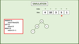
25. SIMULATION
0 1 2 3 4
3
5 4 1
10
Index
Data
10
5 3
4 1
Swap
Swapping the first
element with the last
element of unsorted
array
Heapify(A, i)
{
l <- left(i)
r <- right(i)
if l <= heapsize[A] and A[l] > A[i]
then largest <- l
else largest <- i
if r <= heapsize[A] and A[r] > A[largest]
then largest <- r
if largest != i
then swap A[i] <-A[largest]
Heapify(A, largest)
}
Buildheap(A)
{
heapsize[A] length[A]
for i |length[A]/2
do Heapify(A, i)
}
Heapsort(A)
{
Buildheap(A)
for i  length[A]
do swap A[1]  A[i]
heapsize[A]  heapsize[A] - 1
Heapify(A, 1)
}

26. SIMULATION
0 1 2 3 4
3
5 4 10
1
Index
Data
1
5 3
4 10 Deleting the last element as sorted
Heapify(A, i)
{
l <- left(i)
r <- right(i)
if l <= heapsize[A] and A[l] > A[i]
then largest <- l
else largest <- i
if r <= heapsize[A] and A[r] > A[largest]
then largest <- r
if largest != i
then swap A[i] <-A[largest]
Heapify(A, largest)
}
Buildheap(A)
{
heapsize[A] length[A]
for i |length[A]/2
do Heapify(A, i)
}
Heapsort(A)
{
Buildheap(A)
for i  length[A]
do swap A[1]  A[i]
heapsize[A]  heapsize[A] - 1
Heapify(A, 1)
}

27. SIMULATION
0 1 2 3 4
3
5 4 10
1
Index
Data
1
5 3
4
Sorted Array
Heapify(A, i)
{
l <- left(i)
r <- right(i)
if l <= heapsize[A] and A[l] > A[i]
then largest <- l
else largest <- i
if r <= heapsize[A] and A[r] > A[largest]
then largest <- r
if largest != i
then swap A[i] <-A[largest]
Heapify(A, largest)
}
Buildheap(A)
{
heapsize[A] length[A]
for i |length[A]/2
do Heapify(A, i)
}
Heapsort(A)
{
Buildheap(A)
for i  length[A]
do swap A[1]  A[i]
heapsize[A]  heapsize[A] - 1
Heapify(A, 1)
}

28. SIMULATION
0 1 2 3 4
3
5 4 10
1
Index
Data
1
5 3
4
Calling Heapify
Heapify(A, i)
{
l <- left(i)
r <- right(i)
if l <= heapsize[A] and A[l] > A[i]
then largest <- l
else largest <- i
if r <= heapsize[A] and A[r] > A[largest]
then largest <- r
if largest != i
then swap A[i] <-A[largest]
Heapify(A, largest)
}
Buildheap(A)
{
heapsize[A] length[A]
for i |length[A]/2
do Heapify(A, i)
}
Heapsort(A)
{
Buildheap(A)
for i  length[A]
do swap A[1]  A[i]
heapsize[A]  heapsize[A] - 1
Heapify(A, 1)
}

29. SIMULATION
0 1 2 3 4
3
5 4 10
1
Index
Data
1
5 3
4
5 is greater than 1
then swap A[i] <-A[largest]
Swap 5 and 1
Swap
Heapify(A, i)
{
l <- left(i)
r <- right(i)
if l <= heapsize[A] and A[l] > A[i]
then largest <- l
else largest <- i
if r <= heapsize[A] and A[r] > A[largest]
then largest <- r
if largest != i
then swap A[i] <-A[largest]
Heapify(A, largest)
}
Buildheap(A)
{
heapsize[A] length[A]
for i |length[A]/2
do Heapify(A, i)
}
Heapsort(A)
{
Buildheap(A)
for i  length[A]
do swap A[1]  A[i]
heapsize[A]  heapsize[A] - 1
Heapify(A, 1)
}

30. SIMULATION
0 1 2 3 4
3
1 4 10
5
Index
Data
5
1 3
4
5 is greater than 1
then swap A[i] <-A[largest]
Swap 5 and 1
Heapify(A, i)
{
l <- left(i)
r <- right(i)
if l <= heapsize[A] and A[l] > A[i]
then largest <- l
else largest <- i
if r <= heapsize[A] and A[r] > A[largest]
then largest <- r
if largest != i
then swap A[i] <-A[largest]
Heapify(A, largest)
}
Buildheap(A)
{
heapsize[A] length[A]
for i |length[A]/2
do Heapify(A, i)
}
Heapsort(A)
{
Buildheap(A)
for i  length[A]
do swap A[1]  A[i]
heapsize[A]  heapsize[A] - 1
Heapify(A, 1)
}

31. SIMULATION
0 1 2 3 4
3
1 4 10
5
Index
Data
5
1 3
4
4 is greater than 1
then swap A[i] <-A[largest]
Swap 4 and 1
Swap
Heapify(A, i)
{
l <- left(i)
r <- right(i)
if l <= heapsize[A] and A[l] > A[i]
then largest <- l
else largest <- i
if r <= heapsize[A] and A[r] > A[largest]
then largest <- r
if largest != i
then swap A[i] <-A[largest]
Heapify(A, largest)
}
Buildheap(A)
{
heapsize[A] length[A]
for i |length[A]/2
do Heapify(A, i)
}
Heapsort(A)
{
Buildheap(A)
for i  length[A]
do swap A[1]  A[i]
heapsize[A]  heapsize[A] - 1
Heapify(A, 1)
}

32. SIMULATION
0 1 2 3 4
3
4 1 10
5
Index
Data
5
4 3
1
Heapify(A, i)
{
l <- left(i)
r <- right(i)
if l <= heapsize[A] and A[l] > A[i]
then largest <- l
else largest <- i
if r <= heapsize[A] and A[r] > A[largest]
then largest <- r
if largest != i
then swap A[i] <-A[largest]
Heapify(A, largest)
}
Buildheap(A)
{
heapsize[A] length[A]
for i |length[A]/2
do Heapify(A, i)
}
Heapsort(A)
{
Buildheap(A)
for i  length[A]
do swap A[1]  A[i]
heapsize[A]  heapsize[A] - 1
Heapify(A, 1)
}

33. Swap
SIMULATION
0 1 2 3 4
3
4 1 10
5
Index
Data
5
4 3
1
Swapping the first
element with the last
element of unsorted
array and delete the
last element as
sorted
Heapify(A, i)
{
l <- left(i)
r <- right(i)
if l <= heapsize[A] and A[l] > A[i]
then largest <- l
else largest <- i
if r <= heapsize[A] and A[r] > A[largest]
then largest <- r
if largest != i
then swap A[i] <-A[largest]
Heapify(A, largest)
}
Buildheap(A)
{
heapsize[A] length[A]
for i |length[A]/2
do Heapify(A, i)
}
Heapsort(A)
{
Buildheap(A)
for i  length[A] //down to 2
do swap A[1]  A[i]
heapsize[A]  heapsize[A] - 1
Heapify(A, 1)
}

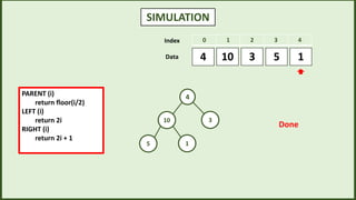
34. SIMULATION
0 1 2 3 4
3
4 5 10
1
Index
Data
1
4 3
Sorted Array
Heapify(A, i)
{
l <- left(i)
r <- right(i)
if l <= heapsize[A] and A[l] > A[i]
then largest <- l
else largest <- i
if r <= heapsize[A] and A[r] > A[largest]
then largest <- r
if largest != i
then swap A[i] <-A[largest]
Heapify(A, largest)
}
Buildheap(A)
{
heapsize[A] length[A]
for i |length[A]/2
do Heapify(A, i)
}
Heapsort(A)
{
Buildheap(A)
for i  length[A]
do swap A[1]  A[i]
heapsize[A]  heapsize[A] - 1
Heapify(A, 1)
}

35. SIMULATION
0 1 2 3 4
3
4 5 10
1
Index
Data
1
4 3
4 is greater than 1
then swap A[i] <-A[largest]
Swap 4 and 1
Swap
Heapify(A, i)
{
l <- left(i)
r <- right(i)
if l <= heapsize[A] and A[l] > A[i]
then largest <- l
else largest <- i
if r <= heapsize[A] and A[r] > A[largest]
then largest <- r
if largest != i
then swap A[i] <-A[largest]
Heapify(A, largest)
}
Buildheap(A)
{
heapsize[A] length[A]
for i |length[A]/2
do Heapify(A, i)
}
Heapsort(A)
{
Buildheap(A)
for i  length[A]
do swap A[1]  A[i]
heapsize[A]  heapsize[A] - 1
Heapify(A, 1)
}

36. SIMULATION
0 1 2 3 4
3
1 5 10
4
Index
Data
4
1 3
Heapify(A, i)
{
l <- left(i)
r <- right(i)
if l <= heapsize[A] and A[l] > A[i]
then largest <- l
else largest <- i
if r <= heapsize[A] and A[r] > A[largest]
then largest <- r
if largest != i
then swap A[i] <-A[largest]
Heapify(A, largest)
}
Buildheap(A)
{
heapsize[A] length[A]
for i |length[A]/2
do Heapify(A, i)
}
Heapsort(A)
{
Buildheap(A)
for i  length[A]
do swap A[1]  A[i]
heapsize[A]  heapsize[A] - 1
Heapify(A, 1)
}

37. SIMULATION
0 1 2 3 4
3
1 5 10
4
Index
Data
4
1 3
Swap
Swapping the first
element with the last
element of unsorted
array and delete the
last element as
sorted
Heapify(A, i)
{
l <- left(i)
r <- right(i)
if l <= heapsize[A] and A[l] > A[i]
then largest <- l
else largest <- i
if r <= heapsize[A] and A[r] > A[largest]
then largest <- r
if largest != i
then swap A[i] <-A[largest]
Heapify(A, largest)
}
Buildheap(A)
{
heapsize[A] length[A]
for i |length[A]/2
do Heapify(A, i)
}
Heapsort(A)
{
Buildheap(A)
for i  length[A]
do swap A[1]  A[i]
heapsize[A]  heapsize[A] - 1
Heapify(A, 1)
}

38. SIMULATION
0 1 2 3 4
4
1 5 10
3
Index
Data
3
1
Build
Heap
Max
Heap
Sort
Continue…

39. SIMULATION
0 1 2 3 4
4
3 5 10
1
Index
Data
The array is sorted

40. Heapify(A, i)
{
l <- left(i)
r <- right(i)
if l <= heapsize[A] and A[l] > A[i]
then largest <- l
else largest <- i
if r <= heapsize[A] and A[r] > A[largest]
then largest <- r
if largest != i
then swap A[i] <-A[largest]
Heapify(A, largest)
}
Buildheap(A)
{
heapsize[A] length[A]
for i |length[A]/2
do Heapify(A, i)
}
Heapsort(A)
{
Buildheap(A)
for i  length[A]
do swap A[1]  A[i]
heapsize[A]  heapsize[A] - 1
Heapify(A, 1)
}
TIME COMPLEXITY ANALYSIS
O (N)
O(log N)
O (N log N)
(n – 1) O(N log N)

41. SPACE COMPLEXITY ANALYSIS
O (1)

42. APPLICATION

43. ADVANTAGES
• No quadratic worst-case run time.
• In-place sorting algorithm, performs sorting in O(1)
space complexity.
• Compared to quicksort, it has a better worst-case time
complexity – O(NlogN).
• The best-case complexity is the same for both quick
and heap sort – O(NlogN).
• Unlike merge sort, it doesn’t require extra space.
• The input data being completely or almost sorted
doesn’t make the complexities suffer.
• The average-case time complexity is the same as that
of merge quick and quick sort

44. DISADVANTAGES
• Heap sort is typically not stable since the operations
on the top can change the relative order of equal key
items. It’s typically an unstable algorithm.
• If the input array is very large and doesn’t fit into the
memory and partitioning the array is faster than
maintaining the heap, heap sort isn’t an option. In
such cases, something like merge sort or bucket sort
where parts of the array can be processed separately
and parallelly, works best.

45. Thank you

46. Doubts?