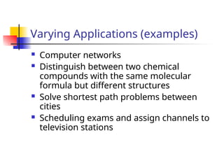
Varying Applications (examples)
Computer networks
Distinguish between two chemical
compounds with the same molecular
formula but different structures
Solve shortest path problems between
cities
Scheduling exams and assign channels to
television stations
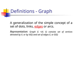
Definitions - Graph
Ageneralization of the simple concept of a
set of dots, links, edges or arcs.
Representation: Graph G =(V, E) consists set of vertices
denoted by V, or by V(G) and set of edges E, or E(G)
5.
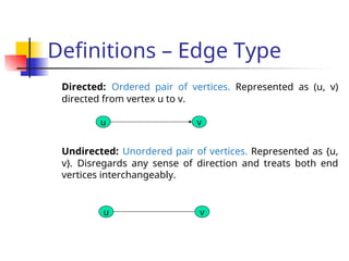
Definitions – EdgeType
Directed: Ordered pair of vertices. Represented as (u, v)
directed from vertex u to v.
Undirected: Unordered pair of vertices. Represented as {u,
v}. Disregards any sense of direction and treats both end
vertices interchangeably.
u v
u v
6.
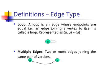
Definitions – EdgeType
Loop: A loop is an edge whose endpoints are
equal i.e., an edge joining a vertex to itself is
called a loop. Represented as {u, u} = {u}
Multiple Edges: Two or more edges joining the
same pair of vertices.
u
u v
7.
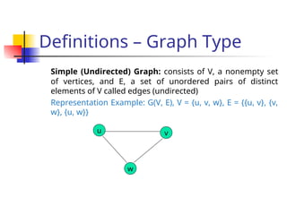
Definitions – GraphType
Simple (Undirected) Graph: consists of V, a nonempty set
of vertices, and E, a set of unordered pairs of distinct
elements of V called edges (undirected)
Representation Example: G(V, E), V = {u, v, w}, E = {{u, v}, {v,
w}, {u, w}}
u v
w
8.
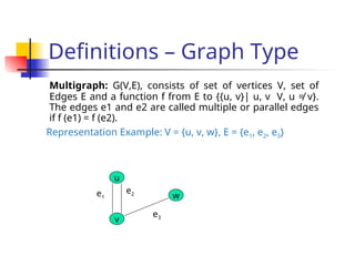
Definitions – GraphType
Multigraph: G(V,E), consists of set of vertices V, set of
Edges E and a function f from E to {{u, v}| u, v V, u ≠ v}.
The edges e1 and e2 are called multiple or parallel edges
if f (e1) = f (e2).
Representation Example: V = {u, v, w}, E = {e1, e2, e3}
u
v
w
e1
e2
e3
9.
Definitions – GraphType
Pseudograph: G(V,E), consists of set of vertices V, set of Edges
E and a function F from E to {{u, v}| u, v Î V}. Loops allowed in
such a graph.
Representation Example: V = {u, v, w}, E = {e1, e2, e3, e4}
u
v
w
e1
e3
e2
e4
10.
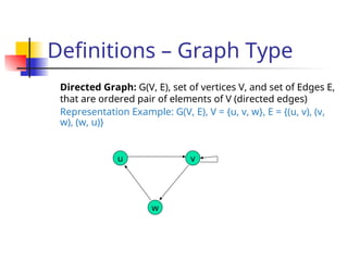
Definitions – GraphType
Directed Graph: G(V, E), set of vertices V, and set of Edges E,
that are ordered pair of elements of V (directed edges)
Representation Example: G(V, E), V = {u, v, w}, E = {(u, v), (v,
w), (w, u)}
u
w
v
11.
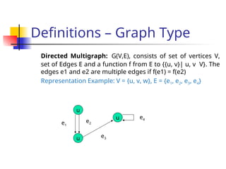
Definitions – GraphType
Directed Multigraph: G(V,E), consists of set of vertices V,
set of Edges E and a function f from E to {{u, v}| u, v V}. The
edges e1 and e2 are multiple edges if f(e1) = f(e2)
Representation Example: V = {u, v, w}, E = {e1, e2, e3, e4}
u
u
u
e1
e2
e3
e4
12.
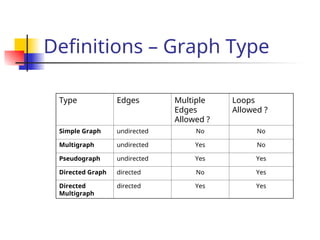
Definitions – GraphType
Type Edges Multiple
Edges
Allowed ?
Loops
Allowed ?
Simple Graph undirected No No
Multigraph undirected Yes No
Pseudograph undirected Yes Yes
Directed Graph directed No Yes
Directed
Multigraph
directed Yes Yes
13.
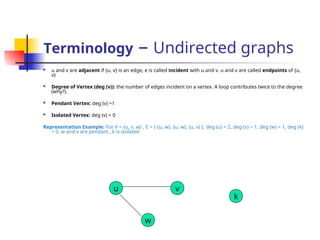
Terminology – Undirectedgraphs
u and v are adjacent if {u, v} is an edge, e is called incident with u and v. u and v are called endpoints of {u,
v}
Degree of Vertex (deg (v)): the number of edges incident on a vertex. A loop contributes twice to the degree
(why?).
Pendant Vertex: deg (v) =1
Isolated Vertex: deg (v) = 0
Representation Example: For V = {u, v, w} , E = { {u, w}, {u, w}, (u, v) }, deg (u) = 2, deg (v) = 1, deg (w) = 1, deg (k)
= 0, w and v are pendant , k is isolated
u
k
w
v
14.
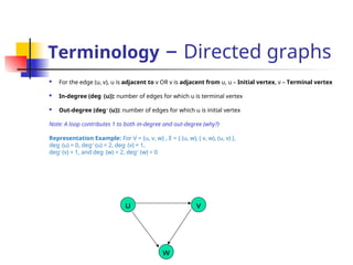
Terminology – Directedgraphs
For the edge (u, v), u is adjacent to v OR v is adjacent from u, u – Initial vertex, v – Terminal vertex
In-degree (deg-
(u)): number of edges for which u is terminal vertex
Out-degree (deg+
(u)): number of edges for which u is initial vertex
Note: A loop contributes 1 to both in-degree and out-degree (why?)
Representation Example: For V = {u, v, w} , E = { (u, w), ( v, w), (u, v) },
deg-
(u) = 0, deg+
(u) = 2, deg-
(v) = 1,
deg+
(v) = 1, and deg-
(w) = 2, deg+
(w) = 0
u
w
v
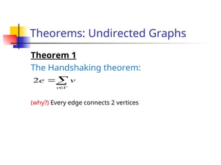
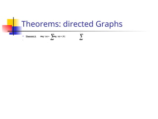
Theorems: Undirected Graphs
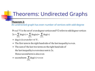
Theorem2:
An undirected graph has even number of vertices with odd degree
even
V
oof
2
2
1
V
v
1,
V
v
V
u
V
v
deg(v)
term
second
even
also
is
term
second
Hence
2e.
is
sum
since
even
is
inequality
last
the
of
side
hand
right
on the
terms
last two
the
of
sum
The
even.
is
inequality
last
the
of
side
hand
right
in the
first term
The
V
for v
even
is
(v)
deg
deg(v)
deg(u)
deg(v)
2e
vertices
degree
odd
to
refers
V2
and
vertices
degree
even
of
set
the
is
1
Pr
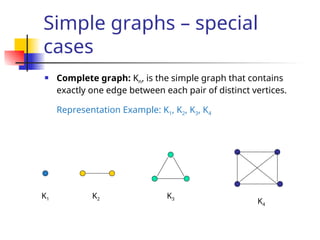
Simple graphs –special
cases
Complete graph: Kn, is the simple graph that contains
exactly one edge between each pair of distinct vertices.
Representation Example: K1, K2, K3, K4
K2
K1
K4
K3
19.
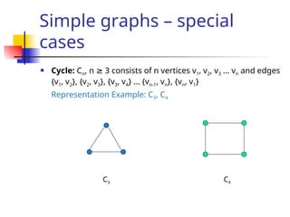
Simple graphs –special
cases
Cycle: Cn, n 3 consists of n vertices v
≥ 1, v2, v3 … vn and edges
{v1, v2}, {v2, v3}, {v3, v4} … {vn-1, vn}, {vn, v1}
Representation Example: C3, C4
C3 C4
20.
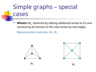
Simple graphs –special
cases
Wheels: Wn, obtained by adding additional vertex to Cn and
connecting all vertices to this new vertex by new edges.
Representation Example: W3, W4
W3 W4
21.
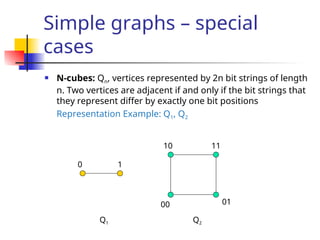
Simple graphs –special
cases
N-cubes: Qn, vertices represented by 2n bit strings of length
n. Two vertices are adjacent if and only if the bit strings that
they represent differ by exactly one bit positions
Representation Example: Q1, Q2
0
10
1
00
11
Q1
01
Q2
22.
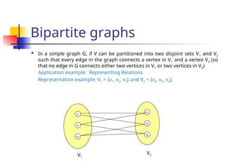
Bipartite graphs
Ina simple graph G, if V can be partitioned into two disjoint sets V1 and V2
such that every edge in the graph connects a vertex in V1 and a vertex V2 (so
that no edge in G connects either two vertices in V1 or two vertices in V2)
Application example: Representing Relations
Representation example: V1 = {v1, v2, v3} and V2 = {v4, v5, v6},
v1
v2
v3
v4
v5
v6
V1
V2
23.
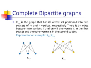
Complete Bipartite graphs
Km,n is the graph that has its vertex set portioned into two
subsets of m and n vertices, respectively There is an edge
between two vertices if and only if one vertex is in the first
subset and the other vertex is in the second subset.
Representation example: K2,3, K3,3
K2,3 K3,3
24.
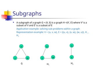
Subgraphs
A subgraphof a graph G = (V, E) is a graph H =(V’, E’) where V’ is a
subset of V and E’ is a subset of E
Application example: solving sub-problems within a graph
Representation example: V = {u, v, w}, E = ({u, v}, {v, w}, {w, u}}, H1 ,
H2
u
v w
u
u
w
v v
H1
H2
G
25.
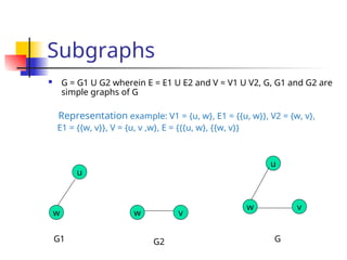
Subgraphs
G =G1 U G2 wherein E = E1 U E2 and V = V1 U V2, G, G1 and G2 are
simple graphs of G
Representation example: V1 = {u, w}, E1 = {{u, w}}, V2 = {w, v},
E1 = {{w, v}}, V = {u, v ,w}, E = {{{u, w}, {{w, v}}
u
v
w w
v
w
u
G1 G2 G
26.
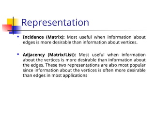
Representation
Incidence (Matrix):Most useful when information about
edges is more desirable than information about vertices.
Adjacency (Matrix/List): Most useful when information
about the vertices is more desirable than information about
the edges. These two representations are also most popular
since information about the vertices is often more desirable
than edges in most applications
27.
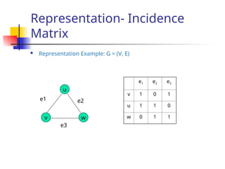
Representation- Incidence
Matrix
G =(V, E) be an undirected graph. Suppose that v1, v2, v3, …, vn are the vertices and e1, e2, …, em are the edges of G. Then the incidence matrix with respect to this ordering of V and E is the nx m
matrix M = [m ij], where
Can also be used to represent :
Multiple edges: by using columns with identical entries, since these edges are incident with the same pair of vertices
Loops: by using a column with exactly one entry equal to 1, corresponding to the vertex that is incident with the loop
otherwise
0
ith v
incident w
is
e
edge
when
1
m
i
j
ij
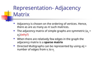
Representation- Adjacency
Matrix
Thereis an N x N matrix, where |V| = N , the Adjacenct Matrix
(NxN) A = [aij]
For undirected graph
For directed graph
This makes it easier to find subgraphs, and to reverse graphs if needed.
otherwise
0
G
of
edge
an
is
)
v
,
(v
if
1
a
j
i
ij
otherwise
0
G
of
edge
an
is
}
v
,
{v
if
1
a
j
i
ij
30.
Representation- Adjacency
Matrix
Adjacencyis chosen on the ordering of vertices. Hence,
there as are as many as n! such matrices.
The adjacency matrix of simple graphs are symmetric (aij =
aji) (why?)
When there are relatively few edges in the graph the
adjacency matrix is a sparse matrix
Directed Multigraphs can be represented by using aij =
number of edges from vi to vj
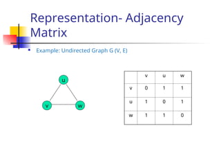
Representation- Adjacency List
Eachnode (vertex) has a list of which nodes (vertex) it is adjacent
Example: undirectd graph G (V, E)
u
v w
nod
e
Adjacency List
u v , w
v w, u
w u , v
34.
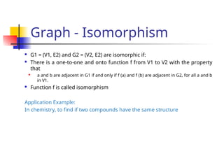
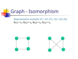
Graph - Isomorphism
G1 = (V1, E2) and G2 = (V2, E2) are isomorphic if:
There is a one-to-one and onto function f from V1 to V2 with the property
that
a and b are adjacent in G1 if and only if f (a) and f (b) are adjacent in G2, for all a and b
in V1.
Function f is called isomorphism
Application Example:
In chemistry, to find if two compounds have the same structure
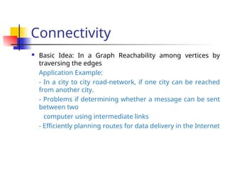
Connectivity
Basic Idea:In a Graph Reachability among vertices by
traversing the edges
Application Example:
- In a city to city road-network, if one city can be reached
from another city.
- Problems if determining whether a message can be sent
between two
computer using intermediate links
- Efficiently planning routes for data delivery in the Internet
37.
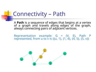
Connectivity – Path
APath is a sequence of edges that begins at a vertex
of a graph and travels along edges of the graph,
always connecting pairs of adjacent vertices.
Representation example: G = (V, E), Path P
represented, from u to v is {{u, 1}, {1, 4}, {4, 5}, {5, v}}
1
u
3
4 5
2
v
38.
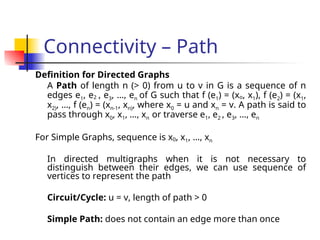
Connectivity – Path
Definitionfor Directed Graphs
A Path of length n (> 0) from u to v in G is a sequence of n
edges e1, e2 , e3, …, en of G such that f (e1) = (xo, x1), f (e2) = (x1,
x2), …, f (en) = (xn-1, xn), where x0 = u and xn = v. A path is said to
pass through x0, x1, …, xn or traverse e1, e2 , e3, …, en
For Simple Graphs, sequence is x0, x1, …, xn
In directed multigraphs when it is not necessary to
distinguish between their edges, we can use sequence of
vertices to represent the path
Circuit/Cycle: u = v, length of path > 0
Simple Path: does not contain an edge more than once
39.
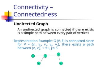
Connectivity –
Connectedness
Undirected Graph
Anundirected graph is connected if there exists
is a simple path between every pair of vertices
Representation Example: G (V, E) is connected since
for V = {v1, v2, v3, v4, v5}, there exists a path
between {vi, vj}, 1 i, j 5
≤ ≤
v1
v2
v3
v5
v4
40.
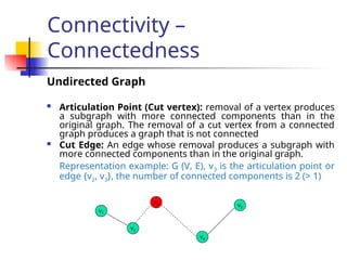
Connectivity –
Connectedness
Undirected Graph
Articulation Point (Cut vertex): removal of a vertex produces
a subgraph with more connected components than in the
original graph. The removal of a cut vertex from a connected
graph produces a graph that is not connected
Cut Edge: An edge whose removal produces a subgraph with
more connected components than in the original graph.
Representation example: G (V, E), v3 is the articulation point or
edge {v2, v3}, the number of connected components is 2 (> 1)
v1
v2
v3
v4
v5
41.
Connectivity –
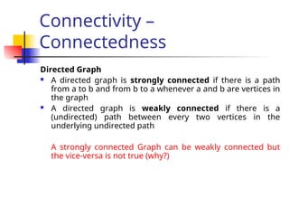
Connectedness
Directed Graph
A directed graph is strongly connected if there is a path
from a to b and from b to a whenever a and b are vertices in
the graph
A directed graph is weakly connected if there is a
(undirected) path between every two vertices in the
underlying undirected path
A strongly connected Graph can be weakly connected but
the vice-versa is not true (why?)
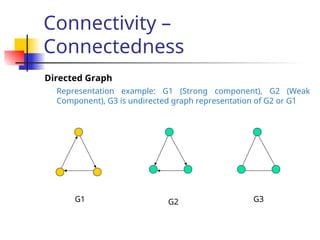
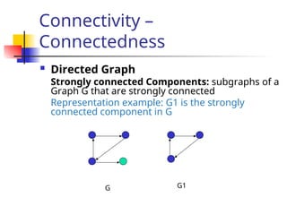
Connectivity –
Connectedness
DirectedGraph
Strongly connected Components: subgraphs of a
Graph G that are strongly connected
Representation example: G1 is the strongly
connected component in G
G1
G
44.
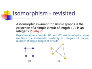
Isomorphism - revisited
Aisomorphic invariant for simple graphs is the
existence of a simple circuit of length k , k is an
integer > 2 (why ?)
Representation example: G1 and G2 are isomorphic since
we have the invariants, similarity in degree of nodes,
number of edges, length of circuits
G1 G2
45.
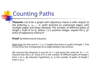
Counting Paths
Theorem:Let G be a graph with adjacency matrix A with respect to
the ordering v1, v2, …, Vn (with directed on undirected edges, with
multiple edges and loops allowed). The number of different paths of
length r from Vi to Vj, where r is a positive integer, equals the (i, j)th
entry of (adjacency matrix) Ar.
Proof: By Mathematical Induction.
Base Case: For the case N = 1, aij =1 implies that there is a path of length 1. This
is true since this corresponds to an edge between two vertices.
We assume that theorem is true for N = r and prove the same for N = r +1.
Assume that the (i, j)th
entry of Ar
is the number of different paths of length r
from vi to vj. By induction hypothesis, bik is the number of paths of length r
from vi to vk.
46.
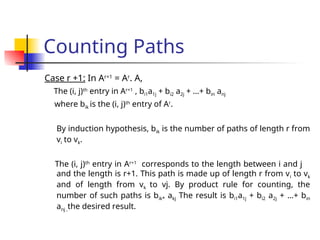
Counting Paths
Case r+1: In Ar+1
= Ar
. A,
The (i, j)th
entry in Ar+1
, bi1a1j + bi2 a2j + …+ bin anj
where bik is the (i, j)th
entry of Ar
.
By induction hypothesis, bik is the number of paths of length r from
vi to vk.
The (i, j)th
entry in Ar+1
corresponds to the length between i and j
and the length is r+1. This path is made up of length r from vi to vk
and of length from vk to vj. By product rule for counting, the
number of such paths is bik* akj The result is bi1a1j + bi2 a2j + …+ bin
anj ,the desired result.
47.
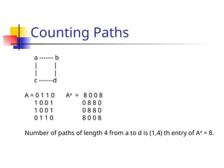
Counting Paths
a -------b
| |
| |
c -------d
A = 0 1 1 0 A4
= 8 0 0 8
1 0 0 1 0 8 8 0
1 0 0 1 0 8 8 0
0 1 1 0 8 0 0 8
Number of paths of length 4 from a to d is (1,4) th entry of A4
= 8.
48.
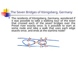
The Seven Bridgesof Königsberg, Germany
The residents of Königsberg, Germany, wondered if
it was possible to take a walking tour of the town
that crossed each of the seven bridges over the
Presel river exactly once. Is it possible to start at
some node and take a walk that uses each edge
exactly once, and ends at the starting node?
49.
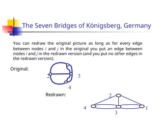
The Seven Bridgesof Königsberg, Germany
You can redraw the original picture as long as for every edge
between nodes i and j in the original you put an edge between
nodes i and j in the redrawn version (and you put no other edges in
the redrawn version).
Original:
2
3
4 1
Redrawn:
4
2 3
50.
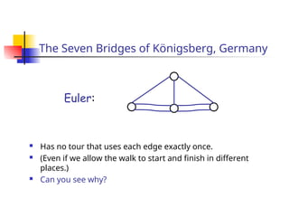
The Seven Bridgesof Königsberg, Germany
Has no tour that uses each edge exactly once.
(Even if we allow the walk to start and finish in different
places.)
Can you see why?
Euler:
51.
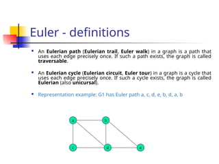
Euler - definitions
An Eulerian path (Eulerian trail, Euler walk) in a graph is a path that
uses each edge precisely once. If such a path exists, the graph is called
traversable.
An Eulerian cycle (Eulerian circuit, Euler tour) in a graph is a cycle that
uses each edge precisely once. If such a cycle exists, the graph is called
Eulerian (also unicursal).
Representation example: G1 has Euler path a, c, d, e, b, d, a, b
a b
c d e
52.
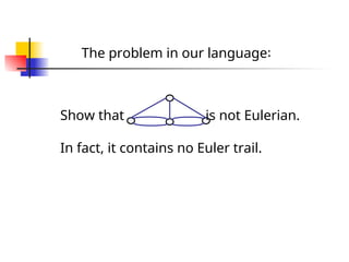
The problem inour language:
Show that is not Eulerian.
In fact, it contains no Euler trail.
53.
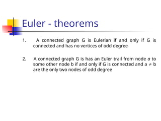
Euler - theorems
1.A connected graph G is Eulerian if and only if G is
connected and has no vertices of odd degree
2. A connected graph G is has an Euler trail from node a to
some other node b if and only if G is connected and a b
are the only two nodes of odd degree
54.
Euler – theorems(=>)
Assume G has an Euler trail T from node a to node b (a and b
not necessarily distinct).
For every node besides a and b, T uses an edge to exit for
each edge it uses to enter. Thus, the degree of the node is
even.
1. If a = b, then a also has even degree. Euler circuit
2. If a b, then a and b both have odd degree. Euler path
55.
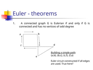
Euler - theorems
1.A connected graph G is Eulerian if and only if G is
connected and has no vertices of odd degree
a b
c d
e
f
Building a simple path:
{a,b}, {b,c}, {c,f}, {f,a}
Euler circuit constructed if all edges
are used. True here?
56.
Euler - theorems
1.A connected graph G is Eulerian if and only if G is
connected and has no vertices of odd degree
c d
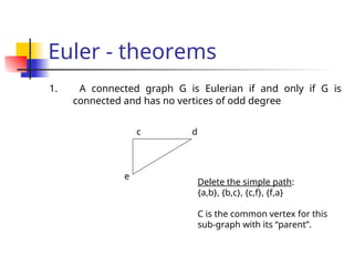
e
Delete the simple path:
{a,b}, {b,c}, {c,f}, {f,a}
C is the common vertex for this
sub-graph with its “parent”.
57.
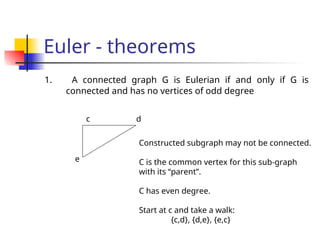
Euler - theorems
1.A connected graph G is Eulerian if and only if G is
connected and has no vertices of odd degree
c d
e
Constructed subgraph may not be connected.
C is the common vertex for this sub-graph
with its “parent”.
C has even degree.
Start at c and take a walk:
{c,d}, {d,e}, {e,c}
58.
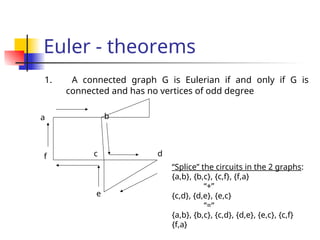
Euler - theorems
1.A connected graph G is Eulerian if and only if G is
connected and has no vertices of odd degree
a b
c d
e
f
“Splice” the circuits in the 2 graphs:
{a,b}, {b,c}, {c,f}, {f,a}
“+”
{c,d}, {d,e}, {e,c}
“=“
{a,b}, {b,c}, {c,d}, {d,e}, {e,c}, {c,f}
{f,a}
59.
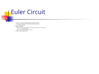
Euler Circuit
1. CircuitC := a circuit in G beginning at an arbitrary vertex v.
1. Add edges successively to form a path that returns to this vertex.
2. H := G – above circuit C
3. While H has edges
1. Sub-circuit sc := a circuit that begins at a vertex in H that is also in C (e.g., vertex “c”)
2. H := H – sc (- all isolated vertices)
3. Circuit := circuit C “spliced” with sub-circuit sc
4. Circuit C has the Euler circuit.
60.
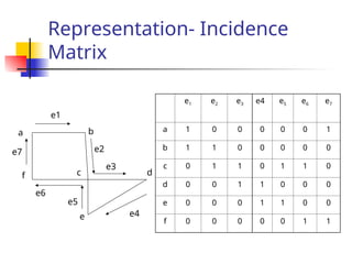
Representation- Incidence
Matrix
e1 e2e3
a 1 0 0
b 1 1 0
c 0 1 1
d 0 0 1
e 0 0 0
f 0 0 0
a b
c d
e
f
e1
e2
e3
e4
e5
e6
e7
e4 e5 e6 e7
0 0 0 1
0 0 0 0
0 1 1 0
1 0 0 0
1 1 0 0
0 0 1 1
61.
Homework 1
Writea program to obtain Euler Circuits.
Input graphs can be Eulerian, no need for checking “non”
Euler graphs
Include a simple user interface to “input” the graph.
Minimum of 10 edges (no more than 15 edges needed)
Simple documentation
Include a sample graph, if needed, to test
Any programming language
Submission on WebCT
Due on January 27th
11.55pm.
62.
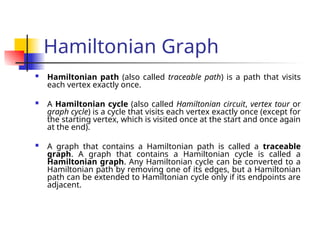
Hamiltonian Graph
Hamiltonianpath (also called traceable path) is a path that visits
each vertex exactly once.
A Hamiltonian cycle (also called Hamiltonian circuit, vertex tour or
graph cycle) is a cycle that visits each vertex exactly once (except for
the starting vertex, which is visited once at the start and once again
at the end).
A graph that contains a Hamiltonian path is called a traceable
graph. A graph that contains a Hamiltonian cycle is called a
Hamiltonian graph. Any Hamiltonian cycle can be converted to a
Hamiltonian path by removing one of its edges, but a Hamiltonian
path can be extended to Hamiltonian cycle only if its endpoints are
adjacent.
63.
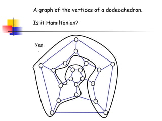
A graph ofthe vertices of a dodecahedron.
Is it Hamiltonian?
Yes
.
64.
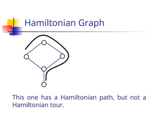
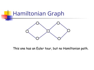
This one hasa Hamiltonian path, but not a
Hamiltonian tour.
Hamiltonian Graph
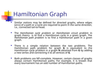
Hamiltonian Graph
Similarnotions may be defined for directed graphs, where edges
(arcs) of a path or a cycle are required to point in the same direction,
i.e., connected tail-to-head.
The Hamiltonian cycle problem or Hamiltonian circuit problem in
graph theory is to find a Hamiltonian cycle in a given graph. The
Hamiltonian path problem is to find a Hamiltonian path in a given
graph.
There is a simple relation between the two problems. The
Hamiltonian path problem for graph G is equivalent to the
Hamiltonian cycle problem in a graph H obtained from G by adding
a new vertex and connecting it to all vertices of G.
Both problems are NP-complete. However, certain classes of graphs
always contain Hamiltonian paths. For example, it is known that
every tournament has an odd number of Hamiltonian paths.
67.
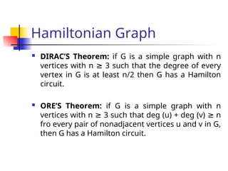
Hamiltonian Graph
DIRAC’STheorem: if G is a simple graph with n
vertices with n 3 such that the degree of every
≥
vertex in G is at least n/2 then G has a Hamilton
circuit.
ORE’S Theorem: if G is a simple graph with n
vertices with n 3 such that deg (u) + deg (v) n
≥ ≥
fro every pair of nonadjacent vertices u and v in G,
then G has a Hamilton circuit.
68.
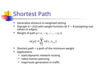
Shortest Path
Generalizedistance to weighted setting
Digraph G = (V,E) with weight function W: E R (assigning real
values to edges)
Weight of path p = v1 v2 … vk is
Shortest path = a path of the minimum weight
Applications
static/dynamic network routing
robot motion planning
map/route generation in traffic
1
1
1
( ) ( , )
k
i i
i
w p w v v
69.
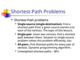
Shortest-Path Problems
Shortest-Pathproblems
Single-source (single-destination). Find a
shortest path from a given source (vertex s) to
each of the vertices. The topic of this lecture.
Single-pair. Given two vertices, find a shortest
path between them. Solution to single-source
problem solves this problem efficiently, too.
All-pairs. Find shortest-paths for every pair of
vertices. Dynamic programming algorithm.
Unweighted shortest-paths – BFS.
70.
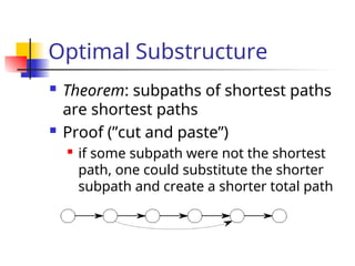
Optimal Substructure
Theorem:subpaths of shortest paths
are shortest paths
Proof (”cut and paste”)
if some subpath were not the shortest
path, one could substitute the shorter
subpath and create a shorter total path
71.
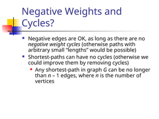
Negative Weights and
Cycles?
Negative edges are OK, as long as there are no
negative weight cycles (otherwise paths with
arbitrary small “lengths” would be possible)
Shortest-paths can have no cycles (otherwise we
could improve them by removing cycles)
Any shortest-path in graph G can be no longer
than n – 1 edges, where n is the number of
vertices
72.
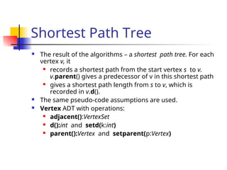
Shortest Path Tree
The result of the algorithms – a shortest path tree. For each
vertex v, it
records a shortest path from the start vertex s to v.
v.parent() gives a predecessor of v in this shortest path
gives a shortest path length from s to v, which is
recorded in v.d().
The same pseudo-code assumptions are used.
Vertex ADT with operations:
adjacent():VertexSet
d():int and setd(k:int)
parent():Vertex and setparent(p:Vertex)
73.
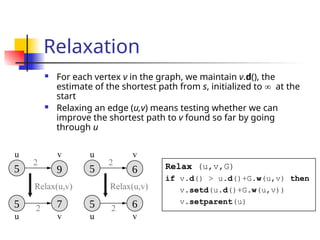
Relaxation
For eachvertex v in the graph, we maintain v.d(), the
estimate of the shortest path from s, initialized to at the
start
Relaxing an edge (u,v) means testing whether we can
improve the shortest path to v found so far by going
through u
u v
v
u
2
2
Relax(u,v)
u v
v
u
2
2
Relax(u,v)
Relax (u,v,G)
if v.d() > u.d()+G.w(u,v) then
v.setd(u.d()+G.w(u,v))
v.setparent(u)
74.
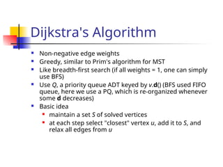
Dijkstra's Algorithm
Non-negativeedge weights
Greedy, similar to Prim's algorithm for MST
Like breadth-first search (if all weights = 1, one can simply
use BFS)
Use Q, a priority queue ADT keyed by v.d() (BFS used FIFO
queue, here we use a PQ, which is re-organized whenever
some d decreases)
Basic idea
maintain a set S of solved vertices
at each step select "closest" vertex u, add it to S, and
relax all edges from u
75.
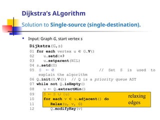
Dijkstra’s ALgorithm
Solution toSingle-source (single-destination).
Input: Graph G, start vertex s
relaxing
edges
Dijkstra(G,s)
01 for each vertex u G.V()
02 u.setd(
03 u.setparent(NIL)
04 s.setd(0)
05 S // Set S is used to
explain the algorithm
06 Q.init(G.V()) // Q is a priority queue ADT
07 while not Q.isEmpty()
08 u Q.extractMin()
09 S S {u}
10 for each v u.adjacent() do
11 Relax(u, v, G)
12 Q.modifyKey(v)
76.
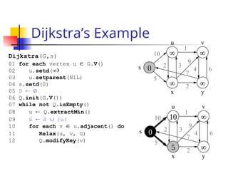
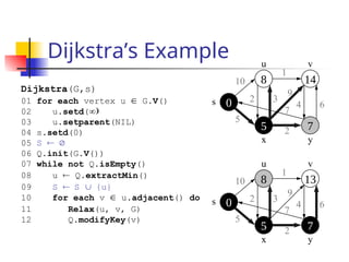
Dijkstra’s Example
s
u v
y
x
10
5
1
2 3
9
4 6
7
2
s
u v
y
x
10
5
1
2 3
9
4 6
7
2
Dijkstra(G,s)
01 for each vertex u G.V()
02 u.setd(
03 u.setparent(NIL)
04 s.setd(0)
05 S
06 Q.init(G.V())
07 while not Q.isEmpty()
08 u Q.extractMin()
09 S S {u}
10 for each v u.adjacent() do
11 Relax(u, v, G)
12 Q.modifyKey(v)
77.
Dijkstra’s Example uv
s
y
x
10
5
1
2 3
9
4 6
7
2
s
u v
y
x
10
5
1
2 3
9
4 6
7
2
Dijkstra(G,s)
01 for each vertex u G.V()
02 u.setd(
03 u.setparent(NIL)
04 s.setd(0)
05 S
06 Q.init(G.V())
07 while not Q.isEmpty()
08 u Q.extractMin()
09 S S {u}
10 for each v u.adjacent() do
11 Relax(u, v, G)
12 Q.modifyKey(v)
78.
Dijkstra’s Example
u v
y
x
10
5
1
2 3
9
4 6
7
2
u v
y
x
10
5
1
2 3
9
4 6
7
2
Dijkstra(G,s)
01 for each vertex u G.V()
02 u.setd(
03 u.setparent(NIL)
04 s.setd(0)
05 S
06 Q.init(G.V())
07 while not Q.isEmpty()
08 u Q.extractMin()
09 S S {u}
10 for each v u.adjacent() do
11 Relax(u, v, G)
12 Q.modifyKey(v)
79.
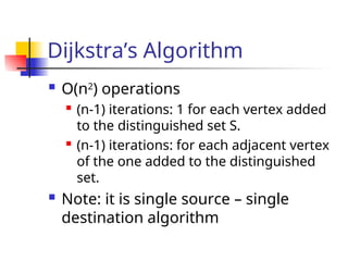
Dijkstra’s Algorithm
O(n2
)operations
(n-1) iterations: 1 for each vertex added
to the distinguished set S.
(n-1) iterations: for each adjacent vertex
of the one added to the distinguished
set.
Note: it is single source – single
destination algorithm
80.
Traveling Salesman Problem
Given a number of cities and the costs of traveling from one
to the other, what is the cheapest roundtrip route that visits
each city once and then returns to the starting city?
An equivalent formulation in terms of graph theory is: Find
the Hamiltonian cycle with the least weight in a weighted
graph.
It can be shown that the requirement of returning to the
starting city does not change the computational complexity
of the problem.
A related problem is the (bottleneck TSP): Find the
Hamiltonian cycle in a weighted graph with the minimal
length of the longest edge.
81.
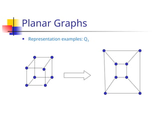
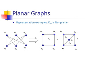
Planar Graphs
Agraph (or multigraph) G is called planar if G can be drawn in the plane
with its edges intersecting only at vertices of G, such a drawing of G is
called an embedding of G in the plane.
Application Example: VLSI design (overlapping edges requires extra
layers), Circuit design (cannot overlap wires on board)
Representation examples: K1,K2,K3,K4 are planar, Kn for n>4 are non-
planar
K4
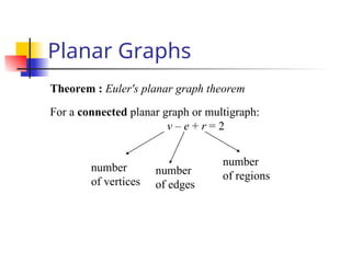
Theorem : Euler'splanar graph theorem
For a connected planar graph or multigraph:
v – e + r = 2
number
of vertices
number
of edges
number
of regions
Planar Graphs
85.
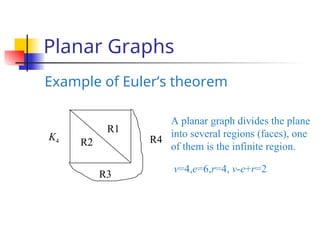
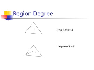
Planar Graphs
Example ofEuler’s theorem
K4
R1
R2
R3
A planar graph divides the plane
into several regions (faces), one
of them is the infinite region.
v=4,e=6,r=4, v-e+r=2
R4
86.
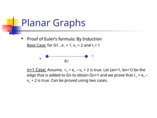
Planar Graphs
Proofof Euler’s formula: By Induction
Base Case: for G1 , e1 = 1, v1 = 2 and r1= 1
n+1 Case: Assume, rn = en – vn + 2 is true. Let {an+1, bn+1} be the
edge that is added to Gn to obtain Gn+1 and we prove that rn = en –
vn + 2 is true. Can be proved using two cases.
R1
v
u
Planar Graphs
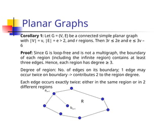
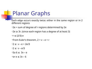
Corollary 1:Let G = (V, E) be a connected simple planar graph
with |V| = v, |E| = e > 2, and r regions. Then 3r 2e and e 3v –
≤ ≤
6
Proof: Since G is loop-free and is not a multigraph, the boundary
of each region (including the infinite region) contains at least
three edges. Hence, each region has degree 3.
≥
Degree of region: No. of edges on its boundary; 1 edge may
occur twice on boundary -> contributes 2 to the region degree.
Each edge occurs exactly twice: either in the same region or in 2
different regions
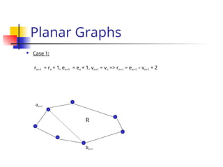
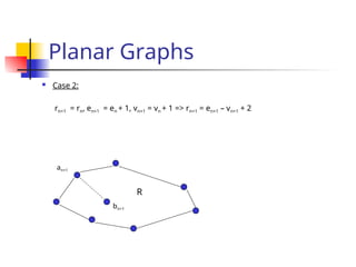
R
an+1
bn+1
Planar Graphs
Each edgeoccurs exactly twice: either in the same region or in 2
different regions
2e = sum of degree of r regions determined by 2e
2e 3r. (since each region has a degree of at least 3)
≥
r (2/3) e
≤
From Euler’s theorem, 2 = v – e + r
2 v – e + 2e/3
≤
2 v – e/3
≤
So 6 3v – e
≤
or e 3v – 6
≤
92.
Planar Graphs
Corollary 2:Let G = (V, E) be a connected simple planar graph
then G has a vertex degree that does not exceed 5
Proof: If G has one or two vertices the result is true
If G has 3 or more vertices then by Corollary 1, e 3v – 6
≤
2e 6v – 12
≤
If the degree of every vertex were at least 6:
by Handshaking theorem: 2e = Sum (deg(v))
2e 6v. But this contradicts the inequality 2e 6v – 12
≥ ≤
There must be at least one vertex with degree no greater than 5
93.
Planar Graphs
Corollary 3:Let G = (V, E) be a connected simple planar graph
with v vertices ( v 3) , e edges, and no circuits of length 3 then
≥
e 2v -4
≤
Proof: Similar to Corollary 1 except the fact that no circuits of
length 3 imply that degree of region must be at least 4.
94.
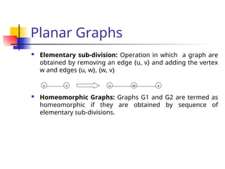
Planar Graphs
Elementarysub-division: Operation in which a graph are
obtained by removing an edge {u, v} and adding the vertex
w and edges {u, w}, {w, v}
Homeomorphic Graphs: Graphs G1 and G2 are termed as
homeomorphic if they are obtained by sequence of
elementary sub-divisions.
u v u v
w
95.
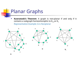
Planar Graphs
Kuwratoski’sTheorem: A graph is non-planar if and only if it
contains a subgraph homeomorephic to K3,3 or K5
Representation Example: G is Nonplanar
a
b
c
j
d
i
e
g
f
k
b
a
c
e
d
f
g
h
G
H K5
e
d
c
b
a
96.
Graph Coloring Problem
Graph coloring is an assignment of "colors", almost always
taken to be consecutive integers starting from 1 without loss
of generality, to certain objects in a graph. Such objects can
be vertices, edges, faces, or a mixture of the above.
Application examples: scheduling, register allocation in a
microprocessor, frequency assignment in mobile radios, and
pattern matching
97.
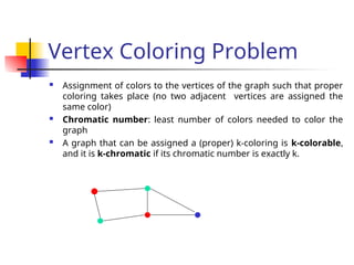
Vertex Coloring Problem
Assignment of colors to the vertices of the graph such that proper
coloring takes place (no two adjacent vertices are assigned the
same color)
Chromatic number: least number of colors needed to color the
graph
A graph that can be assigned a (proper) k-coloring is k-colorable,
and it is k-chromatic if its chromatic number is exactly k.
98.
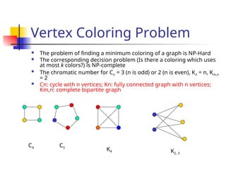
Vertex Coloring Problem
The problem of finding a minimum coloring of a graph is NP-Hard
The corresponding decision problem (Is there a coloring which uses
at most k colors?) is NP-complete
The chromatic number for Cn = 3 (n is odd) or 2 (n is even), Kn = n, Km,n
= 2
Cn: cycle with n vertices; Kn: fully connected graph with n vertices;
Km,n: complete bipartite graph
C5
K4 K2, 3
C4
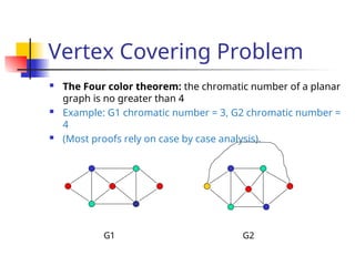
99.
Vertex Covering Problem
The Four color theorem: the chromatic number of a planar
graph is no greater than 4
Example: G1 chromatic number = 3, G2 chromatic number =
4
(Most proofs rely on case by case analysis).
G1 G2


![Representation- Incidence
Matrix
G = (V, E) be an undirected graph. Suppose that v1, v2, v3, …, vn are the vertices and e1, e2, …, em are the edges of G. Then the incidence matrix with respect to this ordering of V and E is the nx m
matrix M = [m ij], where
Can also be used to represent :
Multiple edges: by using columns with identical entries, since these edges are incident with the same pair of vertices
Loops: by using a column with exactly one entry equal to 1, corresponding to the vertex that is incident with the loop
otherwise
0
ith v
incident w
is
e
edge
when
1
m
i
j
ij](https://image.slidesharecdn.com/gtl7graph-250528033950-88e2fb12/85/GT-L7-graph-ppt-Graph-Theory-Discrete-Mathematics-27-320.jpg)
![Representation- Adjacency
Matrix
There is an N x N matrix, where |V| = N , the Adjacenct Matrix
(NxN) A = [aij]
For undirected graph
For directed graph
This makes it easier to find subgraphs, and to reverse graphs if needed.
otherwise
0
G
of
edge
an
is
)
v
,
(v
if
1
a
j
i
ij
otherwise
0
G
of
edge
an
is
}
v
,
{v
if
1
a
j
i
ij](https://image.slidesharecdn.com/gtl7graph-250528033950-88e2fb12/85/GT-L7-graph-ppt-Graph-Theory-Discrete-Mathematics-29-320.jpg)