Download as PDF, PPTX


![Lewis &
Yannakakis
[1980]
The vertex-deletion problem is NP-complete for non-trivial,
hereditary properties.](https://image.slidesharecdn.com/g5csnepyspc0ltr6s0dn-signature-589a2e0a828d35c778544bfcd9130f953b90843638b793665c1663a7419e6a74-poli-141214233504-conversion-gate02/85/Graph-Modification-Algorithms-42-320.jpg)
![Lewis &
Yannakakis
[1980]
The vertex-deletion problem is NP-complete for non-trivial,
hereditary properties.
Yannakakis
[1979]
The connected vertex-deletion problem is NP-complete for
non-trivial properties that hold on connected induced
subgraphs.](https://image.slidesharecdn.com/g5csnepyspc0ltr6s0dn-signature-589a2e0a828d35c778544bfcd9130f953b90843638b793665c1663a7419e6a74-poli-141214233504-conversion-gate02/85/Graph-Modification-Algorithms-43-320.jpg)
![Lewis &
Yannakakis
[1980]
The vertex-deletion problem is NP-complete for non-trivial,
hereditary properties.
Yannakakis
[1979]
(Edgeless, Acyclic, etc.)
The connected vertex-deletion problem is NP-complete for
non-trivial properties that hold on connected induced
subgraphs.](https://image.slidesharecdn.com/g5csnepyspc0ltr6s0dn-signature-589a2e0a828d35c778544bfcd9130f953b90843638b793665c1663a7419e6a74-poli-141214233504-conversion-gate02/85/Graph-Modification-Algorithms-44-320.jpg)
![Lewis &
Yannakakis
[1980]
The vertex-deletion problem is NP-complete for non-trivial,
hereditary properties.
Yannakakis
[1979]
(Edgeless, Acyclic, etc.)
The connected vertex-deletion problem is NP-complete for
non-trivial properties that hold on connected induced
subgraphs.(
Trees, Stars, etc.)](https://image.slidesharecdn.com/g5csnepyspc0ltr6s0dn-signature-589a2e0a828d35c778544bfcd9130f953b90843638b793665c1663a7419e6a74-poli-141214233504-conversion-gate02/85/Graph-Modification-Algorithms-45-320.jpg)


![Edge-Deletion or Completion problems are sometimes easier than their
vertex-deletion counterparts.
Add edges to make the input graph a cluster graph.
Remove edges to make the input graph edgeless.
Remove edges to make the input graph acyclic.
Alon, Shapira
& Sudakov
[2009]
Given a property ᴨ such that ᴨ holds for every
bipartite graph, the Minimum ᴨ-Deletion problem is NP-hard.](https://image.slidesharecdn.com/g5csnepyspc0ltr6s0dn-signature-589a2e0a828d35c778544bfcd9130f953b90843638b793665c1663a7419e6a74-poli-141214233504-conversion-gate02/85/Graph-Modification-Algorithms-53-320.jpg)
![Edge-Deletion or Completion problems are sometimes easier than their
vertex-deletion counterparts.
Add edges to make the input graph a cluster graph.
Remove edges to make the input graph edgeless.
Remove edges to make the input graph acyclic.
Alon, Shapira
& Sudakov
[2009]
Given a property ᴨ such that ᴨ holds for every
bipartite graph, the Minimum ᴨ-Deletion problem is NP-hard.
(Triangle-free)](https://image.slidesharecdn.com/g5csnepyspc0ltr6s0dn-signature-589a2e0a828d35c778544bfcd9130f953b90843638b793665c1663a7419e6a74-poli-141214233504-conversion-gate02/85/Graph-Modification-Algorithms-54-320.jpg)
![Edge-Deletion or Completion problems are sometimes easier than their
vertex-deletion counterparts.
Add edges to make the input graph a cluster graph.
Remove edges to make the input graph edgeless.
Remove edges to make the input graph acyclic.
Alon, Shapira
& Sudakov
[2009]
Given a property ᴨ such that ᴨ holds for every
bipartite graph, the Minimum ᴨ-Deletion problem is NP-hard.
Colbourn &
El-Mallah
[1988]
(Triangle-free)
Making a graph Pk-free by deleting the minimum number of
edges is NP-hard for every k > 2.](https://image.slidesharecdn.com/g5csnepyspc0ltr6s0dn-signature-589a2e0a828d35c778544bfcd9130f953b90843638b793665c1663a7419e6a74-poli-141214233504-conversion-gate02/85/Graph-Modification-Algorithms-55-320.jpg)


![Consider the property ᴨ of being wheel-free, that is,
not having any wheel as an induced subgraph.
Wheel-Free Deletion and Wheel-Free Vertex Deletion
are W[2]-hard.
Lokshtanov
(2008)](https://image.slidesharecdn.com/g5csnepyspc0ltr6s0dn-signature-589a2e0a828d35c778544bfcd9130f953b90843638b793665c1663a7419e6a74-poli-141214233504-conversion-gate02/85/Graph-Modification-Algorithms-83-320.jpg)


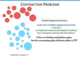
![Finding large induced subgraphs with property ᴨ.
Khot and Raman, (2002)
If ᴨ is a hereditary property that contains all independent sets and all cliques,
or if ᴨ excludes some independent sets and some cliques,
then the problem of finding an induced subgraph of size at least k, satisfying ᴨ,
is FPT.
If ᴨ is a hereditary property contains all independent sets but not all cliques
(or vice versa),
then the problem of finding an induced subgraph of size at least k, satisfying ᴨ,
is W[1]-hard.](https://image.slidesharecdn.com/g5csnepyspc0ltr6s0dn-signature-589a2e0a828d35c778544bfcd9130f953b90843638b793665c1663a7419e6a74-poli-141214233504-conversion-gate02/85/Graph-Modification-Algorithms-86-320.jpg)
![Finding large induced subgraphs with property ᴨ.
Khot and Raman, (2002)
If ᴨ is a hereditary property that contains all independent sets and all cliques,
or if ᴨ excludes some independent sets and some cliques,
then the problem of finding an induced subgraph of size at least k, satisfying ᴨ,
is FPT.
If ᴨ is a hereditary property contains all independent sets but not all cliques
(or vice versa),
then the problem of finding an induced subgraph of size at least k, satisfying ᴨ,
is W[1]-hard.
Ramsey Numbers!
Reduction from Independent Set](https://image.slidesharecdn.com/g5csnepyspc0ltr6s0dn-signature-589a2e0a828d35c778544bfcd9130f953b90843638b793665c1663a7419e6a74-poli-141214233504-conversion-gate02/85/Graph-Modification-Algorithms-87-320.jpg)


![Thanks to Graph Minors, we have a f(k)n2 algorithm for the 퓕-Deletion problem.
For Planar 퓕-Deletion, the starting point was a double-exponential algorithm.
[Bodlaender, 1997]](https://image.slidesharecdn.com/g5csnepyspc0ltr6s0dn-signature-589a2e0a828d35c778544bfcd9130f953b90843638b793665c1663a7419e6a74-poli-141214233504-conversion-gate02/85/Graph-Modification-Algorithms-143-320.jpg)
![Thanks to Graph Minors, we have a f(k)n2 algorithm for the 퓕-Deletion problem.
For Planar 퓕-Deletion, the starting point was a double-exponential algorithm.
[Bodlaender, 1997]
Many single-exponential algorithms are known for special cases of 퓕.](https://image.slidesharecdn.com/g5csnepyspc0ltr6s0dn-signature-589a2e0a828d35c778544bfcd9130f953b90843638b793665c1663a7419e6a74-poli-141214233504-conversion-gate02/85/Graph-Modification-Algorithms-144-320.jpg)
![Thanks to Graph Minors, we have a f(k)n2 algorithm for the 퓕-Deletion problem.
For Planar 퓕-Deletion, the starting point was a double-exponential algorithm.
[Bodlaender, 1997]
Many single-exponential algorithms are known for special cases of 퓕.
Feedback Vertex Set has Cao, Chen & Liu a O*(3.83k) algorithm.
[2010]](https://image.slidesharecdn.com/g5csnepyspc0ltr6s0dn-signature-589a2e0a828d35c778544bfcd9130f953b90843638b793665c1663a7419e6a74-poli-141214233504-conversion-gate02/85/Graph-Modification-Algorithms-145-320.jpg)
![Thanks to Graph Minors, we have a f(k)n2 algorithm for the 퓕-Deletion problem.
For Planar 퓕-Deletion, the starting point was a double-exponential algorithm.
[Bodlaender, 1997]
Many single-exponential algorithms are known for special cases of 퓕.
Cao, Chen & Liu Feedback Vertex Set has a O*(3.83k) algorithm.
[2010]
{K4}-Deletion has Kim, Paul & Philip a O*(2O(k)) algorithm.
[2012]](https://image.slidesharecdn.com/g5csnepyspc0ltr6s0dn-signature-589a2e0a828d35c778544bfcd9130f953b90843638b793665c1663a7419e6a74-poli-141214233504-conversion-gate02/85/Graph-Modification-Algorithms-146-320.jpg)
![Thanks to Graph Minors, we have a f(k)n2 algorithm for the 퓕-Deletion problem.
For Planar 퓕-Deletion, the starting point was a double-exponential algorithm.
[Bodlaender, 1997]
Many single-exponential algorithms are known for special cases of 퓕.
Cao, Chen & Liu Feedback Vertex Set has a O*(3.83k) algorithm.
[2010]
{K4}-Deletion has Kim, Paul & Philip a O*(2O(k)) algorithm.
Pathwidth-1-Deletion has a O*(4.65k) algorithm.
[2012]
Cygan, Pilipczuk,
Pilipczuk & Wojtaszczyk
[2010]](https://image.slidesharecdn.com/g5csnepyspc0ltr6s0dn-signature-589a2e0a828d35c778544bfcd9130f953b90843638b793665c1663a7419e6a74-poli-141214233504-conversion-gate02/85/Graph-Modification-Algorithms-147-320.jpg)

![Fomin, Lokshtanov,
M. & Saurabh
[2013]
Planar퓕-Deletion admits a randomized (2O(k)n) algorithm
when every graph in퓕is connected.](https://image.slidesharecdn.com/g5csnepyspc0ltr6s0dn-signature-589a2e0a828d35c778544bfcd9130f953b90843638b793665c1663a7419e6a74-poli-141214233504-conversion-gate02/85/Graph-Modification-Algorithms-149-320.jpg)
![Fomin, Lokshtanov,
M. & Saurabh
[2013]
Planar퓕-Deletion admits a randomized (2O(k)n) algorithm
when every graph in퓕is connected.
Best possible under ETH.](https://image.slidesharecdn.com/g5csnepyspc0ltr6s0dn-signature-589a2e0a828d35c778544bfcd9130f953b90843638b793665c1663a7419e6a74-poli-141214233504-conversion-gate02/85/Graph-Modification-Algorithms-150-320.jpg)
![Fomin, Lokshtanov,
M. & Saurabh
[2013]
Planar퓕-Deletion admits a randomized (2O(k)n) algorithm
when every graph in퓕is connected.
Best possible under ETH.
Planar 퓕-Deletion admits a deterministic (2O(k)n log2n) algorithm
when every graph in 퓕 is connected.](https://image.slidesharecdn.com/g5csnepyspc0ltr6s0dn-signature-589a2e0a828d35c778544bfcd9130f953b90843638b793665c1663a7419e6a74-poli-141214233504-conversion-gate02/85/Graph-Modification-Algorithms-151-320.jpg)
![Fomin, Lokshtanov,
M. & Saurabh
[2013]
Planar퓕-Deletion admits a randomized (2O(k)n) algorithm
when every graph in퓕is connected.
Best possible under ETH.
Planar 퓕-Deletion admits a deterministic (2O(k)n log2n) algorithm
when every graph in 퓕 is connected.
Planar퓕-Deletion admits an O(nm) randomized algorithm
that leads us to a constant-factor approximation.
Can we get a deterministic
constant-factor approximation algorithm?](https://image.slidesharecdn.com/g5csnepyspc0ltr6s0dn-signature-589a2e0a828d35c778544bfcd9130f953b90843638b793665c1663a7419e6a74-poli-141214233504-conversion-gate02/85/Graph-Modification-Algorithms-152-320.jpg)
![Fomin, Lokshtanov,
M. & Saurabh
[2013]
Planar퓕-Deletion admits a randomized (2O(k)n) algorithm
when every graph in퓕is connected.
Best possible under ETH.
Planar 퓕-Deletion admits a deterministic (2O(k)n log2n) algorithm
when every graph in 퓕 is connected.
Planar퓕-Deletion admits an O(nm) randomized algorithm
that leads us to a constant-factor approximation.
Can we get a deterministic
constant-factor approximation algorithm?
Planar퓕-Deletion admits an deterministic algorithm
that leads us to a O(log3/2(OPT)) approximation.
Fomin, Lokshtanov,
M., Philip & Saurabh
[2013]](https://image.slidesharecdn.com/g5csnepyspc0ltr6s0dn-signature-589a2e0a828d35c778544bfcd9130f953b90843638b793665c1663a7419e6a74-poli-141214233504-conversion-gate02/85/Graph-Modification-Algorithms-153-320.jpg)
![Fomin, Lokshtanov,
M. & Saurabh
[2013]
Planar퓕-Deletion admits a randomized (2O(k)n) algorithm
when every graph in퓕is connected.
Best possible under ETH.
Planar 퓕-Deletion admits a deterministic (2O(k)n log2n) algorithm
when every graph in 퓕 is connected.
Planar퓕-Deletion admits an O(nm) randomized algorithm
that leads us to a constant-factor approximation.
Can we get a deterministic
constant-factor approximation algorithm?
Planar퓕-Deletion admits an deterministic algorithm
that leads us to a O(log3/2(OPT)) approximation.
Fomin, Lokshtanov,
M., Philip & Saurabh
[2013]
Kim, Langer, Paul, Reidl,
Rossmanith, Sau, & Sikdar
[2013]
Planar퓕-Deletion admits a deterministic (2O(k)n2) algorithm.](https://image.slidesharecdn.com/g5csnepyspc0ltr6s0dn-signature-589a2e0a828d35c778544bfcd9130f953b90843638b793665c1663a7419e6a74-poli-141214233504-conversion-gate02/85/Graph-Modification-Algorithms-154-320.jpg)
![Fomin, Lokshtanov,
M. & Saurabh
[2013]
Planar퓕-Deletion admits a randomized (2O(k)n) algorithm
when every graph in퓕is connected.
Best possible under ETH.
Planar 퓕-Deletion admits a deterministic (2O(k)n) algorithm
when every graph in 퓕 is connected.
Planar퓕-Deletion admits an O(nm) randomized algorithm
that leads us to a constant-factor approximation.
Can we get a deterministic
constant-factor approximation algorithm?
Planar퓕-Deletion admits an deterministic algorithm
that leads us to a O(log3/2(OPT)) approximation.
Fomin, Lokshtanov,
M., Philip & Saurabh
[2013]
Kim, Langer, Paul, Reidl,
Rossmanith, Sau, & Sikdar
[2013]
Planar퓕-Deletion admits a deterministic (2O(k)n2) algorithm.
Fomin, Lokshtanov,
M., Ramanujan& Saurabh
[2015]](https://image.slidesharecdn.com/g5csnepyspc0ltr6s0dn-signature-589a2e0a828d35c778544bfcd9130f953b90843638b793665c1663a7419e6a74-poli-141214233504-conversion-gate02/85/Graph-Modification-Algorithms-155-320.jpg)

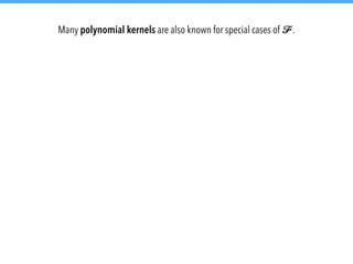
![Many polynomial kernels are also known for special cases of 퓕.
Feedback Vertex Set has a Thomasse O(k2) instance kernel.
[2009]](https://image.slidesharecdn.com/g5csnepyspc0ltr6s0dn-signature-589a2e0a828d35c778544bfcd9130f953b90843638b793665c1663a7419e6a74-poli-141214233504-conversion-gate02/85/Graph-Modification-Algorithms-158-320.jpg)
![Many polynomial kernels are also known for special cases of 퓕.
Thomasse Feedback Vertex Set has a O(k2) instance kernel.
[2009]
Vertex Cover has (Various) a O(k) vertex kernel.](https://image.slidesharecdn.com/g5csnepyspc0ltr6s0dn-signature-589a2e0a828d35c778544bfcd9130f953b90843638b793665c1663a7419e6a74-poli-141214233504-conversion-gate02/85/Graph-Modification-Algorithms-159-320.jpg)
![Many polynomial kernels are also known for special cases of 퓕.
Thomasse Feedback Vertex Set has a O(k2) instance kernel.
[2009]
Vertex Cover has (Various) a O(k) vertex kernel.
Pathwidth-1-Deletion has a polynomial kernel
Cygan, Pilipczuk,
Pilipczuk & Wojtaszczyk
[2010]](https://image.slidesharecdn.com/g5csnepyspc0ltr6s0dn-signature-589a2e0a828d35c778544bfcd9130f953b90843638b793665c1663a7419e6a74-poli-141214233504-conversion-gate02/85/Graph-Modification-Algorithms-160-320.jpg)
![Many polynomial kernels are also known for special cases of 퓕.
Thomasse Feedback Vertex Set has a O(k2) instance kernel.
[2009]
Vertex Cover has (Various) a O(k) vertex kernel.
Pathwidth-1-Deletion has a polynomial kernel
Cygan, Pilipczuk,
Pilipczuk & Wojtaszczyk
[2010]
Fomin, Lokshtanov,
M. & Saurabh
[2013]
Planar 퓕-Deletion admits a polynomial kernel.](https://image.slidesharecdn.com/g5csnepyspc0ltr6s0dn-signature-589a2e0a828d35c778544bfcd9130f953b90843638b793665c1663a7419e6a74-poli-141214233504-conversion-gate02/85/Graph-Modification-Algorithms-161-320.jpg)
![Many polynomial kernels are also known for special cases of 퓕.
Thomasse Feedback Vertex Set has a O(k2) instance kernel.
[2009]
Vertex Cover has (Various) a O(k) vertex kernel.
Pathwidth-1-Deletion has a polynomial kernel
Cygan, Pilipczuk,
Pilipczuk & Wojtaszczyk
[2010]
Fomin, Lokshtanov,
M. & Saurabh
[2013]
Planar 퓕-Deletion admits a polynomial kernel.
Best possible under standard assumptions.](https://image.slidesharecdn.com/g5csnepyspc0ltr6s0dn-signature-589a2e0a828d35c778544bfcd9130f953b90843638b793665c1663a7419e6a74-poli-141214233504-conversion-gate02/85/Graph-Modification-Algorithms-162-320.jpg)

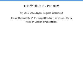
![The 퓕-Deletion Problem
Very little is known beyond the graph minors result.
The most fundamental 퓕-deletion problem that is not accounted for by
Planar 퓕-Deletion is Planarization.
Marx and Schlotter
[2012]
Planarization admits an algorithm with running time
O(2g(k)n2) where g(k) = kO(k3)](https://image.slidesharecdn.com/g5csnepyspc0ltr6s0dn-signature-589a2e0a828d35c778544bfcd9130f953b90843638b793665c1663a7419e6a74-poli-141214233504-conversion-gate02/85/Graph-Modification-Algorithms-166-320.jpg)
![The 퓕-Deletion Problem
Very little is known beyond the graph minors result.
The most fundamental 퓕-deletion problem that is not accounted for by
Planar 퓕-Deletion is Planarization.
Marx and Schlotter
[2012]
Planarization admits an algorithm with running time
O(2g(k)n2) where g(k) = kO(k3)
Kawarabayashi
[2009]
Planarization admits an algorithm with running time
O(f(k)n) where f(k) is not explicitly specified.](https://image.slidesharecdn.com/g5csnepyspc0ltr6s0dn-signature-589a2e0a828d35c778544bfcd9130f953b90843638b793665c1663a7419e6a74-poli-141214233504-conversion-gate02/85/Graph-Modification-Algorithms-167-320.jpg)
![The 퓕-Deletion Problem
Very little is known beyond the graph minors result.
The most fundamental 퓕-deletion problem that is not accounted for by
Planar 퓕-Deletion is Planarization.
Marx and Schlotter
[2012]
Planarization admits an algorithm with running time
O(2g(k)n2) where g(k) = kO(k3)
Kawarabayashi
[2009]
Planarization admits an algorithm with running time
O(f(k)n) where f(k) is not explicitly specified.
Jansen, Lokshtanov &
Saurabh
[2014]
Planarization admits an algorithm with running time
2O(k log k)n, achieving the best combined dependence on k and n.](https://image.slidesharecdn.com/g5csnepyspc0ltr6s0dn-signature-589a2e0a828d35c778544bfcd9130f953b90843638b793665c1663a7419e6a74-poli-141214233504-conversion-gate02/85/Graph-Modification-Algorithms-168-320.jpg)
![The 퓕-Deletion Problem
Very little is known beyond the graph minors result.
The most fundamental 퓕-deletion problem that is not accounted for by
Planar 퓕-Deletion is Planarization.
The question of kernels is completely open.
Marx and Schlotter
[2012]
Planarization admits an algorithm with running time
O(2g(k)n2) where g(k) = kO(k3)
Kawarabayashi
[2009]
Planarization admits an algorithm with running time
O(f(k)n) where f(k) is not explicitly specified.
Jansen, Lokshtanov &
Saurabh
[2014]
Planarization admits an algorithm with running time
2O(k log k)n, achieving the best combined dependence on k and n.](https://image.slidesharecdn.com/g5csnepyspc0ltr6s0dn-signature-589a2e0a828d35c778544bfcd9130f953b90843638b793665c1663a7419e6a74-poli-141214233504-conversion-gate02/85/Graph-Modification-Algorithms-169-320.jpg)


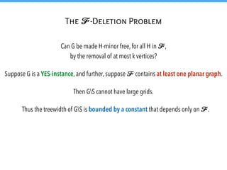
![Contraction To C4-free graphs
Can G be made C4-free by the contraction of at most k edges?
W[2]-hard by a simple reduction from Hitting Set.](https://image.slidesharecdn.com/g5csnepyspc0ltr6s0dn-signature-589a2e0a828d35c778544bfcd9130f953b90843638b793665c1663a7419e6a74-poli-141214233504-conversion-gate02/85/Graph-Modification-Algorithms-174-320.jpg)
![Contraction To C4-free graphs
Can G be made C4-free by the contraction of at most k edges?
W[2]-hard by a simple reduction from Hitting Set.](https://image.slidesharecdn.com/g5csnepyspc0ltr6s0dn-signature-589a2e0a828d35c778544bfcd9130f953b90843638b793665c1663a7419e6a74-poli-141214233504-conversion-gate02/85/Graph-Modification-Algorithms-175-320.jpg)

![Ct-free Contraction isW[2]-hard if t ⩾ 4 and FPT if t⩽ 3.
Pt-free Contraction isW[2]-hard if t ⩾ 5 and FPT if t ⩽ 4.
Lokshtanov, M. &
Saurabh
[2013]](https://image.slidesharecdn.com/g5csnepyspc0ltr6s0dn-signature-589a2e0a828d35c778544bfcd9130f953b90843638b793665c1663a7419e6a74-poli-141214233504-conversion-gate02/85/Graph-Modification-Algorithms-177-320.jpg)
![Ct-free Contraction isW[2]-hard if t ⩾ 4 and FPT if t⩽ 3.
Pt-free Contraction isW[2]-hard if t ⩾ 5 and FPT if t ⩽ 4.
Lokshtanov, M. &
Saurabh
[2013]
Chordal Contraction isW[2]-hard while Clique contraction is FPT
but is unlikely to admit a polynomial kernel.
Cai and Guo
[2013]](https://image.slidesharecdn.com/g5csnepyspc0ltr6s0dn-signature-589a2e0a828d35c778544bfcd9130f953b90843638b793665c1663a7419e6a74-poli-141214233504-conversion-gate02/85/Graph-Modification-Algorithms-178-320.jpg)
![Ct-free Contraction isW[2]-hard if t ⩾ 4 and FPT if t⩽ 3.
Pt-free Contraction isW[2]-hard if t ⩾ 5 and FPT if t ⩽ 4.
Lokshtanov, M. &
Saurabh
[2013]
Chordal Contraction isW[2]-hard while Clique contraction is FPT
but is unlikely to admit a polynomial kernel.
Characeterizations are open.
Cai and Guo
[2013]](https://image.slidesharecdn.com/g5csnepyspc0ltr6s0dn-signature-589a2e0a828d35c778544bfcd9130f953b90843638b793665c1663a7419e6a74-poli-141214233504-conversion-gate02/85/Graph-Modification-Algorithms-179-320.jpg)
![Heggernes, van’t Hof,
Lokshtanov & Paul
[2011]
Ct-free Contraction isW[2]-hard if t ⩾ 4 and FPT if t⩽ 3.
Pt-free Contraction isW[2]-hard if t ⩾ 5 and FPT if t ⩽ 4.
Chordal Contraction isW[2]-hard while Clique contraction is FPT
but is unlikely to admit a polynomial kernel.
Contracting to Bipartite graphs is fixed-parameter tractable with
a double-exponential running time.
Lokshtanov, M. &
Saurabh
[2013]
Characeterizations are open.
Cai and Guo
[2013]](https://image.slidesharecdn.com/g5csnepyspc0ltr6s0dn-signature-589a2e0a828d35c778544bfcd9130f953b90843638b793665c1663a7419e6a74-poli-141214233504-conversion-gate02/85/Graph-Modification-Algorithms-180-320.jpg)
![Heggernes, van’t Hof,
Lokshtanov & Paul
[2011]
Ct-free Contraction isW[2]-hard if t ⩾ 4 and FPT if t⩽ 3.
Pt-free Contraction isW[2]-hard if t ⩾ 5 and FPT if t ⩽ 4.
Chordal Contraction isW[2]-hard while Clique contraction is FPT
but is unlikely to admit a polynomial kernel.
Characeterizations are open.
Contracting to Bipartite graphs is fixed-parameter tractable with
a double-exponential running time.
Lokshtanov, M. &
Saurabh
[2013]
Polynomial kernels are open.
Cai and Guo
[2013]](https://image.slidesharecdn.com/g5csnepyspc0ltr6s0dn-signature-589a2e0a828d35c778544bfcd9130f953b90843638b793665c1663a7419e6a74-poli-141214233504-conversion-gate02/85/Graph-Modification-Algorithms-181-320.jpg)
![Heggernes, van’t Hof,
Lokshtanov & Paul
[2011]
Ct-free Contraction isW[2]-hard if t ⩾ 4 and FPT if t⩽ 3.
Pt-free Contraction isW[2]-hard if t ⩾ 5 and FPT if t ⩽ 4.
Chordal Contraction isW[2]-hard while Clique contraction is FPT
but is unlikely to admit a polynomial kernel.
Characeterizations are open.
Contracting to Bipartite graphs is fixed-parameter tractable with
a double-exponential running time.
Lokshtanov, M. &
Saurabh
[2013]
Polynomial kernels are open.
Heggernes, van’t Hof,
Lévêque, Lokshtanov
& Paul
[2011]
Contracting to paths is FPT and has a linear-vertex kernel; while
contracting to trees is FPT but is unlikely to admit a polynomial kernel.
Cai and Guo
[2013]](https://image.slidesharecdn.com/g5csnepyspc0ltr6s0dn-signature-589a2e0a828d35c778544bfcd9130f953b90843638b793665c1663a7419e6a74-poli-141214233504-conversion-gate02/85/Graph-Modification-Algorithms-182-320.jpg)

![Yannakakis
[1981]
Chordal Completion
The minimum fill-in problem is NP-complete
(was left open in the first edition of Garey and Johnson).](https://image.slidesharecdn.com/g5csnepyspc0ltr6s0dn-signature-589a2e0a828d35c778544bfcd9130f953b90843638b793665c1663a7419e6a74-poli-141214233504-conversion-gate02/85/Graph-Modification-Algorithms-185-320.jpg)
![Yannakakis
[1981]
Chordal Completion
The minimum fill-in problem is NP-complete
(was left open in the first edition of Garey and Johnson).
Kaplan, Shamir &
Tarjan
[1999]
Chordal Completion is fixed-parameter tractable (FPT) with
a running time of O(k616k + k2mn).](https://image.slidesharecdn.com/g5csnepyspc0ltr6s0dn-signature-589a2e0a828d35c778544bfcd9130f953b90843638b793665c1663a7419e6a74-poli-141214233504-conversion-gate02/85/Graph-Modification-Algorithms-186-320.jpg)
![Yannakakis
[1981]
Chordal Completion
The minimum fill-in problem is NP-complete
(was left open in the first edition of Garey and Johnson).
Kaplan, Shamir &
Tarjan
[1999]
Chordal Completion is fixed-parameter tractable (FPT) with
a running time of O(k616k + k2mn).
Bodlaender,
Heggernes, & Villanger
[2011]
Chordal Completion is fixed-parameter tractable (FPT) with
a running time of O(2.36k + k2mn).](https://image.slidesharecdn.com/g5csnepyspc0ltr6s0dn-signature-589a2e0a828d35c778544bfcd9130f953b90843638b793665c1663a7419e6a74-poli-141214233504-conversion-gate02/85/Graph-Modification-Algorithms-187-320.jpg)
![Yannakakis
[1981]
Chordal Completion
The minimum fill-in problem is NP-complete
(was left open in the first edition of Garey and Johnson).
Kaplan, Shamir &
Tarjan
[1999]
Chordal Completion is fixed-parameter tractable (FPT) with
a running time of O(k616k + k2mn).
Bodlaender,
Heggernes, & Villanger
[2011]
Chordal Completion is fixed-parameter tractable (FPT) with
a running time of O(2.36k + k2mn).
Fomin & Villanger
[2013]
Chordal Completion admits a sub exponential
parameterized algorithm with a running time of O(2√k log k + k2mn).](https://image.slidesharecdn.com/g5csnepyspc0ltr6s0dn-signature-589a2e0a828d35c778544bfcd9130f953b90843638b793665c1663a7419e6a74-poli-141214233504-conversion-gate02/85/Graph-Modification-Algorithms-188-320.jpg)

![Kaplan, Shamir &
Tarjan
[1999]
Interval Completion
Chordal Completion, Strongly Chordal Completion, and
Proper Interval Completion are fixed-parameter tractable (FPT).](https://image.slidesharecdn.com/g5csnepyspc0ltr6s0dn-signature-589a2e0a828d35c778544bfcd9130f953b90843638b793665c1663a7419e6a74-poli-141214233504-conversion-gate02/85/Graph-Modification-Algorithms-190-320.jpg)
![Kaplan, Shamir &
Tarjan
[1999]
Interval Completion
Chordal Completion, Strongly Chordal Completion, and
Proper Interval Completion are fixed-parameter tractable (FPT).
Heggernes, Paul,
Telle & Villanger
[2007]
Interval Completion is fixed-parameter tractable (FPT),
with a running time of O(k2kn3m).](https://image.slidesharecdn.com/g5csnepyspc0ltr6s0dn-signature-589a2e0a828d35c778544bfcd9130f953b90843638b793665c1663a7419e6a74-poli-141214233504-conversion-gate02/85/Graph-Modification-Algorithms-191-320.jpg)
![Kaplan, Shamir &
Tarjan
[1999]
Interval Completion
Chordal Completion, Strongly Chordal Completion, and
Proper Interval Completion are fixed-parameter tractable (FPT).
Heggernes, Paul,
Telle & Villanger
[2007]
Interval Completion is fixed-parameter tractable (FPT),
with a running time of O(k2kn3m).
Cao
[2007]
Interval Completion has a single-exponential parameterized algorithm,
with a running time of O(6k(n+m)).](https://image.slidesharecdn.com/g5csnepyspc0ltr6s0dn-signature-589a2e0a828d35c778544bfcd9130f953b90843638b793665c1663a7419e6a74-poli-141214233504-conversion-gate02/85/Graph-Modification-Algorithms-192-320.jpg)
![Kaplan, Shamir &
Tarjan
[1999]
Interval Completion
Chordal Completion, Strongly Chordal Completion, and
Proper Interval Completion are fixed-parameter tractable (FPT).
Heggernes, Paul,
Telle & Villanger
[2007]
Interval Completion is fixed-parameter tractable (FPT),
with a running time of O(k2kn3m).
Cao
[2007]
Interval Completion has a single-exponential parameterized algorithm,
with a running time of O(6k(n+m)).
Bliznets, Fomin,
Pilipczuk & Pilipczuk
[2014]
Interval Completion admits a subexponential parameterized algorithm
with a running time of kO(√k)nO(1).](https://image.slidesharecdn.com/g5csnepyspc0ltr6s0dn-signature-589a2e0a828d35c778544bfcd9130f953b90843638b793665c1663a7419e6a74-poli-141214233504-conversion-gate02/85/Graph-Modification-Algorithms-193-320.jpg)


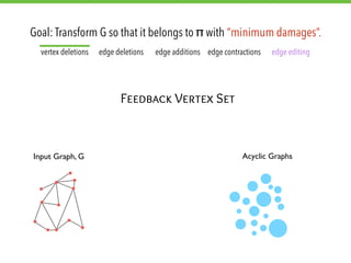
The document explores graph modification problems, focusing on the goal of transforming an input graph to belong to a specified class or property with minimal changes. It discusses various modification operations, such as vertex deletions and edge additions, and their implications on different graph classes and properties. Additionally, the document touches on algorithmic complexity and problem-solving approaches related to graph classification and modification.


![Human Reproduction [ Reproductive System ] Notes @irfanullah_mehar Irfanullah...](https://cdn.slidesharecdn.com/ss_thumbnails/humanreproductionreproductivesystemnotesirfanullahmeharirfanullahmeharjanantantra-260111172350-56e85778-thumbnail.jpg?width=640&height=640&fit=bounds)


