SlideShare a Scribd company logo
1 of 23
Download to read offline
Page 1 of 23
GeneTools Demonstration Notes
Syngene
A Division of the Synoptics Group
Beacon House
Nuffield Road
Cambridge
CB4 1TF
Tel: +44 (0)1223 727123
Fax: +44 (0)1223 727101
www.syngene.com
Version: January 2009
Page 2 of 23
GeneTools Demonstration Guide
Upon opening an image or transferring an image from GeneSnap to GeneTools, the first
window seen contains the Sample Properties.
There are 4 tabs within the Sample Properties window. The first, General, contains a
thumbnail of the image and a number of options which may be selected by the user.
These options depend upon the type of analysis selected. Analysis type determines the
type of analysis required. There are four options:
Gel should be selected for band detection, molecular weight analysis, peak profiling and
densitometry.
Manual Band Quantification is for specific band densitometry.
Page 3 of 23
Spot Blot will automatically detect gridded or non-gridded spot or slot blots or other
samples with ‘round’ data such as ELISA plates. It will perform densitometry,
thresholding and area comparisons etc.
Colony (pour plate) is for colony counting and analysis.
The other tabs within Sample Properties are as follows:
Information – lists the user name (at time of capture), capture date, unique ID number,
darkroom, camera, lighting and exposure settings.
Acquisition notes and Analysis notes – optional notes which may be added by the
user.
Now we will look at the different analysis types and their content.
GEL
When a Gel document is selected, we are looking at tracks of bands upon an
electrophoresis gel. Before proceeding to analysis, ensure that all information is
correctly entered in the Sample Properties window. Whether the image is fluorescence
(white bands on black background) or absorption (vice versa) is automatically detected
– but always check it is correct. The direction of electrophoresis is defaulted to Down
(this can be changed under individual preferences) so ensure this is checked.
The ‘Areas of interest’ Columns and Rows boxes need only be altered if analysing a
multi-layer gel, or multiple gels within the same image. The red box or boxes determine
areas of interest for analysis, and these should be set accordingly. Clicking within each
red box enables track detection to be set for that area. The Tracks menu determines
Page 4 of 23
how tracks are located. If ‘Locate tracks automatically’ is selected, GeneTools will use
unique algorithms to determine where tracks are located, even if they are distorted.
Occasionally the detection algorithm will not locate the tracks accurately. Reasons for
this include insufficient resolution and old gels with diffuse bands. (For more information
read the track finding document on the GeneTools CD).
In these cases the ‘Hint’ facility can be used. The red area of interest box should be
positioned as accurately around the tracks as possible (excluding the borders of the gel).
Enter the approximate number of tracks in the selection box and select ‘OK’.
If the user prefers an exact number of tracks can be manually entered (select the
‘Create’ option), this will often require some further manipulation to ensure tracks are
precisely placed.
Gels or layers within the same image may have tracks detected automatically or
manually. It is possible to return to the Sample Properties window and adjust selections
if the tracks are not located to your satisfaction. Simply select the ‘Sample Properties’
option from the toolbar:
If you are analysing a multi-layer gel and wish to change some rows and not others,
ensure the ‘Leave the tracks unchanged’ function is selected for the rows that are
satisfactory.
GeneSnap annotations can be viewed in GeneTools
Annotations that were added to an sgd file in GeneSnap can now be viewed in
GeneTools. By default the annotations are not visible but by selecting ‘Annotations’ from
the ‘View’ menu they become visible. It is not currently possible to add annotations in
GeneTools.
Mouse zoom/pan
All of the analysis types (gel, spotblot, colony counting) now have the standard mouse
zoom/ pan control that we already have in GeneSnap and Dymension. In addition the
zoom buttons are still present. To zoom in on the image, simply left click then roll the
roller ball forwards.
Once tracks have been overlaid automatically or manually they can be manipulated in
many ways. Manipulation can be either for a single track or all tracks. Track width, well
position, dye front and Rf can all be adjusted. Individual tracks can be bent and
distorted into almost any position. To begin manual manipulation, simply click on the
appropriate icon. Once happy with the position of the tracks, they should be locked by
clicking on the padlock icon. A warning will appear before re-calculating data if
appropriate. NB: for descriptions of all the functions of the track adjustment icons see the
track menu.
Track manipulation icons
Page 5 of 23
Any tracks that you do not wish to include in analysis can be removed from results tables
etc. by selecting ‘disable’ from the track menu.
In the lower part of the screen a data table is displayed which can be used to view one
or all tracks at once. Individual peaks within tracks can be added, deleted or adjusted
by clicking in the right hand top pane, which contains the track histogram.
GeneTools enables the user to analyse gels containing both dark and light bands. This
is a unique feature that makes the software suitable for the analysis of Zyma gels. To
invert a track simply select it and use either a right hand mouse click to reveal the ‘invert’
option or use the Track menu.
Align banks of tracks
This option appears in the view menu.
If analysing a gel with tracks running horizontally, this function will rotate them through
90 degrees so they are vertical. This makes the analysis easier to follow on the screen
Once all tracks and bands have been detected there are many analysis options.
Molecular weights and Quantities can easily be calculated if there are known
standards present on the image. Select the lane containing the standards and click on
the Assign Molecular Weight/Quantity Standard icon.
A window will appear which allows the user to enter values for Molecular weights and
Quantities using one of three methods. In the ‘manual’ tab the user simply selects
peaks with known values and assigns the values manually, moving up and down the
track as appropriate with the arrow keys. The ‘from standard’ tab contains a library of
pre-entered standards which may be loaded. Simply ensure that the first peak is
selected before hitting the assign button. If the appropriate standard is not in the library,
Molecular Weight Parameters
Assign Molecular Weight/Quantity Standard
Page 6 of 23
simply edit an existing one or create a new standard. Once created, the new standard
will enter the library for the next analysis. Any standards assigned can be checked in the
curve window before clicking the OK button to accept them. Once entered and assigned,
the molecular weight values will appear in red in the appropriate track result box, and all
unknown peak values will be calculated from them.
If required the base pairs value may be displayed in the track result box. To select this
option right click in the results table and all available options will be displayed.
If more than one set of markers is used the results are based on both sets. This can
help to correct for smiling. If one selects the Molecular Weight Parameters:
Several variables can be applied to data including curve type, distance measurement
and propagation.
Propagation controls how the different standards are utilised. Interpolation helps to
correct for smiling. Alternatively, use the nearest standard to each track or combine
standards if you have both small and large values.
If a Quantity is known for one of the bands on the gel, the others can be calculated from
it. Click on the known band and then on the Assign Quantity icon.
Quantity Calibration Parameters
Assign Quantity
Enter the value for the band in the window. The value will appear in red under a
‘quantity’ column in the data window, and all unknown values are calculated relative to it.
If the Quantity Calibration Parameters icon is selected one can alter the curve type to
Page 7 of 23
enter a number of known standards (increases accuracy) or to enter some units for the
quantity (e.g.nanograms).
Quantity calculations may be made using one calibration curve for the whole image, or
treating each track as a separate sub-image with its own standard curve. Select the
appropriate setting for your sample in ‘quantity calibration parameters’. If choosing the
latter method, it is possible to propagate a quantity across each track, using either peak
number or peak position (Rf) to achieve this. Select your chosen method of propagation
in ‘assign quantity’.
Within Multi-layer gels it is possible to use a quantity calibration standard from one set of
tracks for another set of tracks or indeed another gel. Simply select as appropriate. If the
‘use another track as standard’ box is ticked, the desired track set may then be selected
from the drop down menu.
Band Matching is another component of GeneTools. This function allows bands on a
selected track to be matched against other bands in other tracks on the gel. Matching
may also be carried out by profile, which takes the shape and size of each peak into
account. Click on the Band Matching Parameters icon to select detailed matching
parameters.
Band Matching Parameters
Set Matching Standard
Page 8 of 23
Once happy, select the track of interest and click on the Band Matching icon.
The bands within the selected track will be joined to any matching ones within the set
detection limits. A Dendrogram will also be produced which can be maximised by using
the right hand mouse button. The dendrograms in GeneTools are based on the
Neighbor-joining or UPGMA methods. For more information on these processes please
consult GeneTools online help under the heading ‘Dendrograms’. For further
information concerning matching, view Matching Comparisons, Matching Matrix and
Matching Coefficients in the data table.
To view one or more of the tracks on the same graph, click on the Profile Comparison
icon:
This feature can be used to compare tracks on the same or different gels. This is an
incredibly useful feature and represents a major advantage over most competitor
software. Just ensure that all gels of interest have an image window open within
GeneTools before clicking on profile comparison. Expand the gel icon on the RHS of the
screen by clicking on +. Then double left click on tracks as required adding or removing
them from the graph. Any track may be selected as the reference by selecting it and
clicking on right hand mouse button. The reference track will automatically be added to
the graph but it can be removed although it will remain the reference until unselected or
another track is selected. The track properties may also be selected by clicking the right
hand mouse button.
To alter the scale of the graph, click on the zoom in button. To view the required section
of graph when in zoom use the scroll bar. If wished, up to twelve different colours can be
assigned to tracks under the Extras/ Configuration menu.
Page 9 of 23
The Profile comparison may be exported to Word or saved to clipboard as required
(see later for more details on reporting functions).
Profile view report in Word now reports colour index
In previous version of GeneTools the profile comparison report was missing the colours
when exported to Word. In the latest version the track names are coloured in the
appropriate colour for the profile.
Within Profile comparison there are now many new functions, one of which is the ability
to export the profile as a series of figures into Excel, so that it may be plotted out. To
select this right click on the track and select ‘Export to Excel’.
The profile comparison view has undergone a fairly radical transformation. Where
previously there were two windows for a tree view of the tracks and the profiles
themselves, there are now three windows.
The third window contains two tabs. The first displays the similarity matrix and the
second the dendrogram. The tracks can be broken down into a number of categories,
depending on what options have been set for a particular track:
1) Displayed in the profile window only:- a profile graph symbol and a line showing
the colour of the profile in the comparison window (e.g. track 2).
2) Displayed in profile and used in matching:- a profile symbol and a dendrogram
symbol (e.g. track 11).
3) Not displayed in profile window and not used in matching:- a profile symbol but
no line (e.g. track 6)
4) Not displayed in profile window but used in matching:- Dendrogram symbol only
(e.g. track 3).
If less than three tracks are displayed no similarity matrix or dendrogram is drawn. The
dialog for altering the matching parameters is the same as that in the gel view
(Matching->Parameters). If the matching is performed by bands then a reference track
must be set (red line with a box [e.g. track 1], as previously).
Page 10 of 23
There are now a number of menu items that make displaying/ matching somewhat
easier:
1) Profile->Show all:- Displays all profiles in the current set.
2) Profile->Hide all:- Hides all profiles in the current set.
3) Matching->Include all in matching:- Adds all tracks from a set to the matching.
4) Matching->Exclude all from matching:- Remove all tracks in a set from the
matching.
There are also menu items to show/ hide and include/ exclude on an individual profile
basis.
The Integration Parameters menu also relates to gel analysis.
Page 11 of 23
In this menu various parameters can be adjusted. Baseline correction is defaulted to
the ‘Rolling disk’ option which is popular in the analysis of ethidium bromide stained
gels and coomassie and silver stained protein gels. These gels may have an intrinsically
high background and results are improved dramatically by applying a correction. For this
method the program first calculates the position of the line formed by the centre of a disk
with the set radius rolled along below the profile.
The baseline is then one radius length above this line, and the corrected signal is
measured as the height above this baseline.
Other methods available are:
‘Lowest slope’ (this method uses a line that connects all the points on the profile, using
the lowest possible slope) but several options are provided:
‘Track borders’ uses the border of the track as a background.
‘Track borders and slope’ is a combination method. The signal is corrected for the
track borders, then the lowest slope method is used.
‘None’ will not apply a background correction.
Please note that selecting ‘edit manual baseline’ from the Track menu enables the user
to set a manual baseline.
Peak detection parameters may be altered to modify the sensitivity of automatic
location. Lower the default values to increase sensitivity and vice versa.
Page 12 of 23
The Savitsky-Golay filter is used in integrating the image. The greater the set width the
greater the smoothing effect of the filter.
Detection filters are for use when working with coloured images. Selecting a particular
filter enables analysis of only that colour within the image. To analyse the whole image,
use no filter.
Using Save Sample Defaults under the Extras menu will save all the settings within
Integration Parameters.
To switch back to a saved set of defaults select Load Sample Defaults from the Extras
menu. If necessary GeneTools will automatically re-locate tracks and extract data.
Please note that only one set of sample defaults per analysis type may be saved under a
user name at one time.
MANUAL BAND QUANTIFICATION
This document type should be selected if the user wishes to carry out densitometry
analysis on a typical electrophoresis gel. The function will automatically open with the
rectangular drawing tool selected.
Mouse zoom/pan
All of the analysis types (gel, spotblot, colony counting) now have the standard mouse
zoom/ pan control that we already have in GeneSnap and Dymension. In addition the
zoom buttons are still present. To zoom in on the image, simply left click then roll the
roller ball forwards.
Click and drag on left mouse button to draw around bands of interest. A double left
mouse click will produce a box identical to the last drawn.
Boxes are automatically numbered in order of drawing and will appear, complete with
Raw volume figures, in a data box at the base of the screen (to display various other
properties in this table, click the right-hand mouse button and select options as
required). If you require all sample boxes to be of identical size, select the Spots same
size icon. The boxes will be the same size when the icon is depressed. In manual band
quantification, the default setting is for different sized bands.
If bands are not rectangular, use the ‘freehand drawing’ tool:
Page 13 of 23
Click and hold the left-hand mouse button to draw around the band. Once drawn the
shape can be altered by clicking and dragging on the blue drag handles.
When all required bands have been drawn around click on the Lock Position icon to
prevent accidental changes:
If you require repositioning after locking, you will need to select the Position any spot
icon:
Background correction is set by clicking the icon:
This will produce a window with a drop down menu. The default setting is ‘None’.
For the most accurate analysis it is best to apply a background correction. There are two
choices:
If you select ‘Automatic’, an individual background measurement will be calculated
from the four pixels at the corners of each sample box. This is suitable for most gel
samples whose background is uneven across the image.
If ‘Manual’ is selected, the user can now draw any number of background boxes upon
the image. The background measurement for each data box will now be taken from the
nearest manual background box.
NB: When using this option please ensure that you draw at least one background box on
the sample, do not just select ‘manual’ then click ‘OK’.
To assign a quantity to a known band, click on the Quantity icon.
A window will appear and the calibrated quantity can be entered. Quantities of the other
bands are now automatically calculated. For greater accuracy more than one known
value may be added. To enable this, click on the Quantity Calibration Parameters
icon. A window will appear and the curve type may be altered to allow multiple standard
values. A unit type e.g.: nanograms may also be entered at this stage. To view the
quantity calibration graph click on the tab in the lower half of the screen.
NB: Quantities may also be assigned by using a right hand mouse button click.
Page 14 of 23
Quantity Calibration Parameters
Assign Quantity
Incidence Parameters
Within Manual Band quantification it is possibly to calculate the incidence of bands
based upon upper and lower limits of various parameters. To use this function, click on
the icon:
A window will appear :
Incidence type can be set according to Raw volume, % Total Raw Volume, Pixel Area or
Quantity. The Incidence value range may have an upper and lower cut-off (select two-
value range) or may be greater than or less than an input value. To obtain values to
define incidence, simply click on the appropriate sample box and click ‘Get spot value’.
To display the selected bands, select the Incidence tab in the data window.
Page 15 of 23
SPOT BLOT
Select Spot Blot as document type. A Sample Properties window will appear:
Firstly, select whether the spot type is circle (most usual), or rectangular (slot blot).
This software option will automatically detect spots whether they are in a gridded or
random formation. If your spots are in a grid then select this setting. Please note
however, that you will be unable to add or delete spots from the grid without returning to
the Sample Properties box to amend row and column numbers. If the boxes for numbers
of rows and columns are left blank, GeneTools will search for all spots within the image.
On a poor image or in cases when only part of the array is of interest, enter numbers for
columns and rows to obtain a template that may be adjusted as required.
When happy, click OK and wait for GeneTools to locate spots. Once located, you must
firstly decide whether or not all spots are the same size. Set this by clicking on the icon
Spots same size. When the icon is faded, this is the same-size setting.
The default settings are same-size for gridded arrays, and not for non-gridded arrays.
Page 16 of 23
Mouse zoom/pan
All of the analysis types (gel, spotblot, colony counting) now have the standard mouse
zoom/ pan control that we already have in GeneSnap and Dymension. In addition the
zoom buttons are still present. To zoom in on the image, simply left click then roll the
roller ball forwards.
For a grid, any adjustment in positioning is best made by moving the control point spots.
These spots are shown in red. These will default to be the corner spots. If these are not
visible, click on the appropriate icon:
To alter the control points, double-click on the spot no longer required. The spot will turn
green. To designate another spot as a control point, simply double click. Only three
control points may be used at any one time.
To position individual spots, select the Position any spot icon:
When analysing a non-gridded spot blot, spots can be added by double clicking, and
deleted by right hand mouse button click.
To locate spots based on an intensity threshold, select the Locate spots icon:
Page 17 of 23
A window will be displayed:
Using the mouse, move the red lines on the
Binary threshold to determine which
spots are included in the analysis.
Please note that this tool is most
useful when analysing non-gridded
samples. Spots which are not coloured
blue will not be included in the analysis.
For gridded samples, the spot locator is
useful if spots are of variable size.
Spots that are part of a grid will not be
removed from the results table even
If they are not coloured blue.
Spots can also be selected/rejected by
altering the minimum/maximum pixel
areas.
Background correction is set by clicking the icon:
This will produce a window with a drop down menu. The default setting is ‘None’.
For the most accurate analysis it is best to apply a background correction. There are two
choices:
If you select ‘Automatic’, an individual background measurement will be calculated
from the four corner pixels of each spot. This is suitable for most gel samples whose
background is uneven across the image.
If ‘Manual’ is selected, the user can now draw any number of background boxes upon
the image. The background measurement for each spot will now be taken from the
nearest manual background box.
NB: When using this option please ensure that you draw at least one background box on
the sample, do not just select ‘manual’ then click ‘OK’.
To assign a quantity to a known spot, click on the Assign Quantity icon.
A window will appear and the calibrated quantity can be entered. Quantities of the other
spots are now automatically calculated. For greater accuracy more than one known
value may be added. To enable this, click on the Quantity Calibration Parameters
icon. A window will appear and the curve type may be altered to allow multiple standard
Page 18 of 23
values. A unit type e.g. nanograms may also be entered at this stage. To view the
quantity calibration graph click on the tab in the lower half of the screen.
NB: Quantities may also be assigned by using a right hand mouse button click.
Spot Incidence Parameters
Within Manual Band quantification it is possibly to calculate the incidence of spots based
upon upper and lower limits of various parameters. To use this function, click on the
icon:
A window will appear :
Incidence type can be set according to Raw volume, % Total Raw Volume, Pixel Area or
Quantity. The Incidence value range may have an upper and lower cut-off (select two-
value range) or may be greater than or less than an input value. To obtain values to
define incidence, simply click on the appropriate spot and click ‘Get spot value’.
To display the selected spots, select the Incidence tab in the data window.
COLONY COUNTING
Select Colony option (pour plate) under Sample Properties. Before proceeding to
analysis, select whether you wish to count dark colonies, light colonies or both together.
(A dark colony is determined as one appearing darker than the background media.
Remember that when using transillumination, colonies normally considered light, usually
appear dark against the background agar).
Also select whether your plate type is circular or square.
Quantity Calibration Parameters
Assign Quantity
Page 19 of 23
Upon entering colony counting, your image will appear on the right hand side of the
screen, with all analysis functions to the left.
Mouse zoom/pan
All of the analysis types (gel, spotblot, colony counting) now have the standard mouse
zoom/ pan control that we already have in GeneSnap and Dymension. In addition the
zoom buttons are still present. To zoom in on the image, simply left click then roll the
roller ball forwards.
The first task is to define the frame.
Use the mouse to position the circular frame over the colony plate. Avoid taking the
frame right up to the edges, where shadowing may be mistaken for colonies.
Page 20 of 23
If there are regions within the plate that you do not wish to include, such as areas of
contamination or pen markings, these can be excluded. Select ‘Draw exclude region’
and then use to mouse to draw as accurately as possible around the unwanted region.
This will no longer be included in the analysis. Exclude regions may be adjusted after
drawing if required.
Next, adjust the sensitivity of detection to include all the colonies of interest.
Select ‘Show shapes’ to determine what is being picked up as colonies and to help avoid
picking up shadows or undissolved agar.
Select ‘Hide outlines’ for a better view of colonies detected.
Choose from a range of settings between Very
Low and Very High.
Once happy with sensitivity, click on Separate
Colonies to apply the separation algorithm.
In order to be more specific about which colonies are detected, select Set area limits
tab. Here it is possible to input maximum and minimum colony sizes. It may take some
experimentation to obtain the correct set of parameters for your colony, but once done
these settings can be saved as Sample Defaults (see later)
Maximum and minimum colony size filter can be set from colonies
When the user right-mouse clicks inside a colony, a pop-up menu appears which allows
them to set either the maximum or minimum area for a colony. This sets the area limits
based on the size of the colony underneath the cursor
The Class Split window is used when looking at two
shades of dark or light colonies. Use the mouse to
adjust the red line and split the colonies into two
class types.
Manual Detection
To use the manual detection function, select Add/remove colonies option
Page 21 of 23
This will enable the manual detection option.
For a single colour colony plate have Class 1 selected. Add or delete colonies by double
clicking the left-hand mouse button. Double-clicking an existing colony will delete it,
double clicking elsewhere will add a colony. Class 2 will be required if two colour plates
are being counted.
When printing to the thermal printer within the colony counting package, the image is
printed along with colony counts and % area readings. All of the usual capture settings
are also displayed.
SAMPLE PROPERTIES
If you change your mind about the type of analysis being carried out at any time, simply
click on the Sample Properties icon to return to this window.
REPORT GENERATION
GeneTools is capable of producing a fully GLP compliant report with details of all
analysis carried out. By clicking on Report Setup icon
the required features can be selected or removed. Headings for report setup are
changed under GeneTools configuration in the Extras menu. Default settings from a
previous report may also be imported using this menu.
Review the report prior to printing using the Print Preview icon.
Be aware that to print out your report you must have an A4 printer attached, and this
should be selected prior to viewing the Print preview.
ONE BUTTON WORD TRANSFER
Page 22 of 23
Simply by clicking on the appropriate icon, the entire GeneTools report, including
graphs, will be transferred to Microsoft Word. This is a very powerful function enabling
the end user to have complete flexibility concerning report production and further
analysis.
ONE BUTTON EXCEL TRANSFER
Any data generated in a results table during a GeneTools analysis can be transferred to
Excel with a single mouse click. Simply select the table of interest if appropriate i.e.:
in molecular weight analysis you may want all tracks or a single track or even matching
comparisons. Click on the Excel icon and the displayed data will instantly be dropped
into a spreadsheet, along with capture information to identify the data source.
NB: Obviously, Excel software must be loaded onto the PC you are using! Some older
versions of Excel will not accept data directly. In these instances, firstly save the data
as a CSV file (see below).
SAVING DATA AS CSV (TEXT) FILES
By clicking the appropriate icon it is possible to save data as a CSV (comma separated
variable) file. This can be opened in most software packages.
SAVE TO CLIPBOARD
This icon, when selected in the main GeneTools analysis, will place the image onto
clipboard. This can then be pasted into Word or alternative applications. By right
clicking within the dendrogram, quantity calibration or molecular weight curve windows,
this information may also be placed onto clipboard. This feature adds to the reporting
flexibility of GeneTools.
CONFIGURATION WINDOW
This window, found within the ‘Extras’ drop down menu allows various adjustments to be
made and stored under user preferences. There are four tabs within the menu:
General – for setting of document type, font, auto-location of tracks etc.
Page 23 of 23
Import – for importation of defaults from previous analyses e.g. mol weight, sample
track and report settings.
Colours – to alter the colours of various lines and plots appearing within the analysis
program to suit personal preferences.
Molecular Weight – to import libraries and set the graph default to log or linear.
USER PREFERENCES
These are stored under your username so when returning to GeneTools it is not
necessary to reset various parameters from Sample properties to molecular weight
libraries. To change username select the function from the Extras menu. This function
makes GeneTools the most flexible and user specific analysis package on the market
today.
TUTORIALS
There are now a number of tutorial available within GeneTools to guide the user through
commonly used features such as report generation, quantitation or calculation of
molecular weight. These can be found in the Help menu and require an internet
connection to run.

More Related Content

Viewers also liked

LTF Labortechnik präsentiert: Geldokumentationssysteme von Syngene
LTF Labortechnik präsentiert: Geldokumentationssysteme von SyngeneLTF Labortechnik präsentiert: Geldokumentationssysteme von Syngene
LTF Labortechnik präsentiert: Geldokumentationssysteme von SyngeneLTF Labortechnik GmbH & Co. KG
 
MyGo Pro - das Original! Nur erhältlich bei LTF Labortechnik
MyGo Pro - das Original! Nur erhältlich bei LTF LabortechnikMyGo Pro - das Original! Nur erhältlich bei LTF Labortechnik
MyGo Pro - das Original! Nur erhältlich bei LTF LabortechnikLTF Labortechnik GmbH & Co. KG
 
Rough Cut 2: Evaluation
Rough Cut 2: EvaluationRough Cut 2: Evaluation
Rough Cut 2: Evaluationomar konteh
 
Διερεύνηση χλωριδικής σύνθεσης επιβαρυμένων μεταλλευτικών και μεταλλουργικών ...
Διερεύνηση χλωριδικής σύνθεσης επιβαρυμένων μεταλλευτικών και μεταλλουργικών ...Διερεύνηση χλωριδικής σύνθεσης επιβαρυμένων μεταλλευτικών και μεταλλουργικών ...
Διερεύνηση χλωριδικής σύνθεσης επιβαρυμένων μεταλλευτικών και μεταλλουργικών ...Anastasia Kondyli
 
Tnl college tour
Tnl college tourTnl college tour
Tnl college tourTNLCUY
 
Business ppt-template-014
Business ppt-template-014Business ppt-template-014
Business ppt-template-014Saeed Bhatti
 
Presentación sobre el sofware educativo y plataforma educativa
Presentación sobre el sofware  educativo y plataforma educativaPresentación sobre el sofware  educativo y plataforma educativa
Presentación sobre el sofware educativo y plataforma educativaEmma Amanda Villaman Morrobel
 

Viewers also liked (12)

LTF Labortechnik präsentiert: Geldokumentationssysteme von Syngene
LTF Labortechnik präsentiert: Geldokumentationssysteme von SyngeneLTF Labortechnik präsentiert: Geldokumentationssysteme von Syngene
LTF Labortechnik präsentiert: Geldokumentationssysteme von Syngene
 
RIDASCREEN Weihnachtstestkit der Firma R-Biopharm
RIDASCREEN Weihnachtstestkit der Firma R-BiopharmRIDASCREEN Weihnachtstestkit der Firma R-Biopharm
RIDASCREEN Weihnachtstestkit der Firma R-Biopharm
 
Se sekjen ttg penyesuaian ak guru
Se sekjen ttg penyesuaian ak guruSe sekjen ttg penyesuaian ak guru
Se sekjen ttg penyesuaian ak guru
 
MyGo Pro - das Original! Nur erhältlich bei LTF Labortechnik
MyGo Pro - das Original! Nur erhältlich bei LTF LabortechnikMyGo Pro - das Original! Nur erhältlich bei LTF Labortechnik
MyGo Pro - das Original! Nur erhältlich bei LTF Labortechnik
 
Rough Cut 2: Evaluation
Rough Cut 2: EvaluationRough Cut 2: Evaluation
Rough Cut 2: Evaluation
 
Preguntas
PreguntasPreguntas
Preguntas
 
Διερεύνηση χλωριδικής σύνθεσης επιβαρυμένων μεταλλευτικών και μεταλλουργικών ...
Διερεύνηση χλωριδικής σύνθεσης επιβαρυμένων μεταλλευτικών και μεταλλουργικών ...Διερεύνηση χλωριδικής σύνθεσης επιβαρυμένων μεταλλευτικών και μεταλλουργικών ...
Διερεύνηση χλωριδικής σύνθεσης επιβαρυμένων μεταλλευτικών και μεταλλουργικών ...
 
Tnl college tour
Tnl college tourTnl college tour
Tnl college tour
 
Business ppt-template-014
Business ppt-template-014Business ppt-template-014
Business ppt-template-014
 
Presentación sobre el sofware educativo y plataforma educativa
Presentación sobre el sofware  educativo y plataforma educativaPresentación sobre el sofware  educativo y plataforma educativa
Presentación sobre el sofware educativo y plataforma educativa
 
Semana de mayo
Semana de mayoSemana de mayo
Semana de mayo
 
RIDASCREEN Christmas Testkit from R-Biopharm
RIDASCREEN Christmas Testkit from R-BiopharmRIDASCREEN Christmas Testkit from R-Biopharm
RIDASCREEN Christmas Testkit from R-Biopharm
 

Similar to GeneTools Demonstration Guide Analysis Software Functions

Dips 7.0 whats_new_quick_start_guide
Dips 7.0 whats_new_quick_start_guideDips 7.0 whats_new_quick_start_guide
Dips 7.0 whats_new_quick_start_guideJoaoManuelLucamba
 
Instructions(1) Work through the pages below.(2) Use the us_demog.docx
Instructions(1) Work through the pages below.(2) Use the us_demog.docxInstructions(1) Work through the pages below.(2) Use the us_demog.docx
Instructions(1) Work through the pages below.(2) Use the us_demog.docxdirkrplav
 
Tools for modeling protein 3 d structure
Tools for modeling protein 3 d structureTools for modeling protein 3 d structure
Tools for modeling protein 3 d structurePriyanka Kashyap
 
InnerSoft STATS - Graphs
InnerSoft STATS - GraphsInnerSoft STATS - Graphs
InnerSoft STATS - GraphsInnerSoft
 
Utilização do SGeMS
Utilização do SGeMSUtilização do SGeMS
Utilização do SGeMSAlex Ramires
 
SPSS User Guide
SPSS User GuideSPSS User Guide
SPSS User GuideBrian Bond
 
InnerSoft STATS - Analyze
InnerSoft STATS - AnalyzeInnerSoft STATS - Analyze
InnerSoft STATS - AnalyzeInnerSoft
 
Diffusion Tensor Imaging Analysis-3749
Diffusion Tensor Imaging Analysis-3749Diffusion Tensor Imaging Analysis-3749
Diffusion Tensor Imaging Analysis-3749Kitware Kitware
 
annotation_tutorial_2008
annotation_tutorial_2008annotation_tutorial_2008
annotation_tutorial_2008tutorialsruby
 
annotation_tutorial_2008
annotation_tutorial_2008annotation_tutorial_2008
annotation_tutorial_2008tutorialsruby
 
T - test independent samples
T - test  independent samplesT - test  independent samples
T - test independent samplesAmit Sharma
 
T test independent samples
T test  independent samplesT test  independent samples
T test independent samplesAmit Sharma
 

Similar to GeneTools Demonstration Guide Analysis Software Functions (20)

Dips 7.0 whats_new_quick_start_guide
Dips 7.0 whats_new_quick_start_guideDips 7.0 whats_new_quick_start_guide
Dips 7.0 whats_new_quick_start_guide
 
Instructions(1) Work through the pages below.(2) Use the us_demog.docx
Instructions(1) Work through the pages below.(2) Use the us_demog.docxInstructions(1) Work through the pages below.(2) Use the us_demog.docx
Instructions(1) Work through the pages below.(2) Use the us_demog.docx
 
Tools for modeling protein 3 d structure
Tools for modeling protein 3 d structureTools for modeling protein 3 d structure
Tools for modeling protein 3 d structure
 
InnerSoft STATS - Graphs
InnerSoft STATS - GraphsInnerSoft STATS - Graphs
InnerSoft STATS - Graphs
 
Utilização do SGeMS
Utilização do SGeMSUtilização do SGeMS
Utilização do SGeMS
 
Axis vm stepbystep
Axis vm stepbystepAxis vm stepbystep
Axis vm stepbystep
 
SPSS User Guide
SPSS User GuideSPSS User Guide
SPSS User Guide
 
datacolor spectrophotometer working procedure
datacolor spectrophotometer working procedure datacolor spectrophotometer working procedure
datacolor spectrophotometer working procedure
 
Sampling
SamplingSampling
Sampling
 
Photoshop tools
Photoshop toolsPhotoshop tools
Photoshop tools
 
InnerSoft STATS - Analyze
InnerSoft STATS - AnalyzeInnerSoft STATS - Analyze
InnerSoft STATS - Analyze
 
ERDAS_1.pdf
ERDAS_1.pdfERDAS_1.pdf
ERDAS_1.pdf
 
Spectrophotometer wroking procedur
Spectrophotometer wroking procedurSpectrophotometer wroking procedur
Spectrophotometer wroking procedur
 
Diffusion Tensor Imaging Analysis-3749
Diffusion Tensor Imaging Analysis-3749Diffusion Tensor Imaging Analysis-3749
Diffusion Tensor Imaging Analysis-3749
 
annotation_tutorial_2008
annotation_tutorial_2008annotation_tutorial_2008
annotation_tutorial_2008
 
annotation_tutorial_2008
annotation_tutorial_2008annotation_tutorial_2008
annotation_tutorial_2008
 
UV - VIS SW
UV - VIS SWUV - VIS SW
UV - VIS SW
 
Adobe photoshop
Adobe photoshopAdobe photoshop
Adobe photoshop
 
T - test independent samples
T - test  independent samplesT - test  independent samples
T - test independent samples
 
T test independent samples
T test  independent samplesT test  independent samples
T test independent samples
 

Recently uploaded

Green chemistry and Sustainable development.pptx
Green chemistry  and Sustainable development.pptxGreen chemistry  and Sustainable development.pptx
Green chemistry and Sustainable development.pptxRajatChauhan518211
 
Unlocking the Potential: Deep dive into ocean of Ceramic Magnets.pptx
Unlocking  the Potential: Deep dive into ocean of Ceramic Magnets.pptxUnlocking  the Potential: Deep dive into ocean of Ceramic Magnets.pptx
Unlocking the Potential: Deep dive into ocean of Ceramic Magnets.pptxanandsmhk
 
PossibleEoarcheanRecordsoftheGeomagneticFieldPreservedintheIsuaSupracrustalBe...
PossibleEoarcheanRecordsoftheGeomagneticFieldPreservedintheIsuaSupracrustalBe...PossibleEoarcheanRecordsoftheGeomagneticFieldPreservedintheIsuaSupracrustalBe...
PossibleEoarcheanRecordsoftheGeomagneticFieldPreservedintheIsuaSupracrustalBe...Sérgio Sacani
 
Labelling Requirements and Label Claims for Dietary Supplements and Recommend...
Labelling Requirements and Label Claims for Dietary Supplements and Recommend...Labelling Requirements and Label Claims for Dietary Supplements and Recommend...
Labelling Requirements and Label Claims for Dietary Supplements and Recommend...Lokesh Kothari
 
Pests of cotton_Borer_Pests_Binomics_Dr.UPR.pdf
Pests of cotton_Borer_Pests_Binomics_Dr.UPR.pdfPests of cotton_Borer_Pests_Binomics_Dr.UPR.pdf
Pests of cotton_Borer_Pests_Binomics_Dr.UPR.pdfPirithiRaju
 
Traditional Agroforestry System in India- Shifting Cultivation, Taungya, Home...
Traditional Agroforestry System in India- Shifting Cultivation, Taungya, Home...Traditional Agroforestry System in India- Shifting Cultivation, Taungya, Home...
Traditional Agroforestry System in India- Shifting Cultivation, Taungya, Home...jana861314
 
SOLUBLE PATTERN RECOGNITION RECEPTORS.pptx
SOLUBLE PATTERN RECOGNITION RECEPTORS.pptxSOLUBLE PATTERN RECOGNITION RECEPTORS.pptx
SOLUBLE PATTERN RECOGNITION RECEPTORS.pptxkessiyaTpeter
 
Formation of low mass protostars and their circumstellar disks
Formation of low mass protostars and their circumstellar disksFormation of low mass protostars and their circumstellar disks
Formation of low mass protostars and their circumstellar disksSérgio Sacani
 
Chromatin Structure | EUCHROMATIN | HETEROCHROMATIN
Chromatin Structure | EUCHROMATIN | HETEROCHROMATINChromatin Structure | EUCHROMATIN | HETEROCHROMATIN
Chromatin Structure | EUCHROMATIN | HETEROCHROMATINsankalpkumarsahoo174
 
STERILITY TESTING OF PHARMACEUTICALS ppt by DR.C.P.PRINCE
STERILITY TESTING OF PHARMACEUTICALS ppt by DR.C.P.PRINCESTERILITY TESTING OF PHARMACEUTICALS ppt by DR.C.P.PRINCE
STERILITY TESTING OF PHARMACEUTICALS ppt by DR.C.P.PRINCEPRINCE C P
 
GFP in rDNA Technology (Biotechnology).pptx
GFP in rDNA Technology (Biotechnology).pptxGFP in rDNA Technology (Biotechnology).pptx
GFP in rDNA Technology (Biotechnology).pptxAleenaTreesaSaji
 
Hubble Asteroid Hunter III. Physical properties of newly found asteroids
Hubble Asteroid Hunter III. Physical properties of newly found asteroidsHubble Asteroid Hunter III. Physical properties of newly found asteroids
Hubble Asteroid Hunter III. Physical properties of newly found asteroidsSérgio Sacani
 
Botany 4th semester file By Sumit Kumar yadav.pdf
Botany 4th semester file By Sumit Kumar yadav.pdfBotany 4th semester file By Sumit Kumar yadav.pdf
Botany 4th semester file By Sumit Kumar yadav.pdfSumit Kumar yadav
 
Broad bean, Lima Bean, Jack bean, Ullucus.pptx
Broad bean, Lima Bean, Jack bean, Ullucus.pptxBroad bean, Lima Bean, Jack bean, Ullucus.pptx
Broad bean, Lima Bean, Jack bean, Ullucus.pptxjana861314
 
Zoology 4th semester series (krishna).pdf
Zoology 4th semester series (krishna).pdfZoology 4th semester series (krishna).pdf
Zoology 4th semester series (krishna).pdfSumit Kumar yadav
 
Discovery of an Accretion Streamer and a Slow Wide-angle Outflow around FUOri...
Discovery of an Accretion Streamer and a Slow Wide-angle Outflow around FUOri...Discovery of an Accretion Streamer and a Slow Wide-angle Outflow around FUOri...
Discovery of an Accretion Streamer and a Slow Wide-angle Outflow around FUOri...Sérgio Sacani
 
Botany 4th semester series (krishna).pdf
Botany 4th semester series (krishna).pdfBotany 4th semester series (krishna).pdf
Botany 4th semester series (krishna).pdfSumit Kumar yadav
 
9654467111 Call Girls In Raj Nagar Delhi Short 1500 Night 6000
9654467111 Call Girls In Raj Nagar Delhi Short 1500 Night 60009654467111 Call Girls In Raj Nagar Delhi Short 1500 Night 6000
9654467111 Call Girls In Raj Nagar Delhi Short 1500 Night 6000Sapana Sha
 
Orientation, design and principles of polyhouse
Orientation, design and principles of polyhouseOrientation, design and principles of polyhouse
Orientation, design and principles of polyhousejana861314
 

Recently uploaded (20)

Green chemistry and Sustainable development.pptx
Green chemistry  and Sustainable development.pptxGreen chemistry  and Sustainable development.pptx
Green chemistry and Sustainable development.pptx
 
Unlocking the Potential: Deep dive into ocean of Ceramic Magnets.pptx
Unlocking  the Potential: Deep dive into ocean of Ceramic Magnets.pptxUnlocking  the Potential: Deep dive into ocean of Ceramic Magnets.pptx
Unlocking the Potential: Deep dive into ocean of Ceramic Magnets.pptx
 
PossibleEoarcheanRecordsoftheGeomagneticFieldPreservedintheIsuaSupracrustalBe...
PossibleEoarcheanRecordsoftheGeomagneticFieldPreservedintheIsuaSupracrustalBe...PossibleEoarcheanRecordsoftheGeomagneticFieldPreservedintheIsuaSupracrustalBe...
PossibleEoarcheanRecordsoftheGeomagneticFieldPreservedintheIsuaSupracrustalBe...
 
Labelling Requirements and Label Claims for Dietary Supplements and Recommend...
Labelling Requirements and Label Claims for Dietary Supplements and Recommend...Labelling Requirements and Label Claims for Dietary Supplements and Recommend...
Labelling Requirements and Label Claims for Dietary Supplements and Recommend...
 
Pests of cotton_Borer_Pests_Binomics_Dr.UPR.pdf
Pests of cotton_Borer_Pests_Binomics_Dr.UPR.pdfPests of cotton_Borer_Pests_Binomics_Dr.UPR.pdf
Pests of cotton_Borer_Pests_Binomics_Dr.UPR.pdf
 
Traditional Agroforestry System in India- Shifting Cultivation, Taungya, Home...
Traditional Agroforestry System in India- Shifting Cultivation, Taungya, Home...Traditional Agroforestry System in India- Shifting Cultivation, Taungya, Home...
Traditional Agroforestry System in India- Shifting Cultivation, Taungya, Home...
 
SOLUBLE PATTERN RECOGNITION RECEPTORS.pptx
SOLUBLE PATTERN RECOGNITION RECEPTORS.pptxSOLUBLE PATTERN RECOGNITION RECEPTORS.pptx
SOLUBLE PATTERN RECOGNITION RECEPTORS.pptx
 
Formation of low mass protostars and their circumstellar disks
Formation of low mass protostars and their circumstellar disksFormation of low mass protostars and their circumstellar disks
Formation of low mass protostars and their circumstellar disks
 
Chromatin Structure | EUCHROMATIN | HETEROCHROMATIN
Chromatin Structure | EUCHROMATIN | HETEROCHROMATINChromatin Structure | EUCHROMATIN | HETEROCHROMATIN
Chromatin Structure | EUCHROMATIN | HETEROCHROMATIN
 
STERILITY TESTING OF PHARMACEUTICALS ppt by DR.C.P.PRINCE
STERILITY TESTING OF PHARMACEUTICALS ppt by DR.C.P.PRINCESTERILITY TESTING OF PHARMACEUTICALS ppt by DR.C.P.PRINCE
STERILITY TESTING OF PHARMACEUTICALS ppt by DR.C.P.PRINCE
 
GFP in rDNA Technology (Biotechnology).pptx
GFP in rDNA Technology (Biotechnology).pptxGFP in rDNA Technology (Biotechnology).pptx
GFP in rDNA Technology (Biotechnology).pptx
 
Hubble Asteroid Hunter III. Physical properties of newly found asteroids
Hubble Asteroid Hunter III. Physical properties of newly found asteroidsHubble Asteroid Hunter III. Physical properties of newly found asteroids
Hubble Asteroid Hunter III. Physical properties of newly found asteroids
 
CELL -Structural and Functional unit of life.pdf
CELL -Structural and Functional unit of life.pdfCELL -Structural and Functional unit of life.pdf
CELL -Structural and Functional unit of life.pdf
 
Botany 4th semester file By Sumit Kumar yadav.pdf
Botany 4th semester file By Sumit Kumar yadav.pdfBotany 4th semester file By Sumit Kumar yadav.pdf
Botany 4th semester file By Sumit Kumar yadav.pdf
 
Broad bean, Lima Bean, Jack bean, Ullucus.pptx
Broad bean, Lima Bean, Jack bean, Ullucus.pptxBroad bean, Lima Bean, Jack bean, Ullucus.pptx
Broad bean, Lima Bean, Jack bean, Ullucus.pptx
 
Zoology 4th semester series (krishna).pdf
Zoology 4th semester series (krishna).pdfZoology 4th semester series (krishna).pdf
Zoology 4th semester series (krishna).pdf
 
Discovery of an Accretion Streamer and a Slow Wide-angle Outflow around FUOri...
Discovery of an Accretion Streamer and a Slow Wide-angle Outflow around FUOri...Discovery of an Accretion Streamer and a Slow Wide-angle Outflow around FUOri...
Discovery of an Accretion Streamer and a Slow Wide-angle Outflow around FUOri...
 
Botany 4th semester series (krishna).pdf
Botany 4th semester series (krishna).pdfBotany 4th semester series (krishna).pdf
Botany 4th semester series (krishna).pdf
 
9654467111 Call Girls In Raj Nagar Delhi Short 1500 Night 6000
9654467111 Call Girls In Raj Nagar Delhi Short 1500 Night 60009654467111 Call Girls In Raj Nagar Delhi Short 1500 Night 6000
9654467111 Call Girls In Raj Nagar Delhi Short 1500 Night 6000
 
Orientation, design and principles of polyhouse
Orientation, design and principles of polyhouseOrientation, design and principles of polyhouse
Orientation, design and principles of polyhouse
 

GeneTools Demonstration Guide Analysis Software Functions

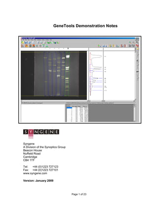
  • 1. Page 1 of 23 GeneTools Demonstration Notes Syngene A Division of the Synoptics Group Beacon House Nuffield Road Cambridge CB4 1TF Tel: +44 (0)1223 727123 Fax: +44 (0)1223 727101 www.syngene.com Version: January 2009
  • 2. Page 2 of 23 GeneTools Demonstration Guide Upon opening an image or transferring an image from GeneSnap to GeneTools, the first window seen contains the Sample Properties. There are 4 tabs within the Sample Properties window. The first, General, contains a thumbnail of the image and a number of options which may be selected by the user. These options depend upon the type of analysis selected. Analysis type determines the type of analysis required. There are four options: Gel should be selected for band detection, molecular weight analysis, peak profiling and densitometry. Manual Band Quantification is for specific band densitometry.
  • 3. Page 3 of 23 Spot Blot will automatically detect gridded or non-gridded spot or slot blots or other samples with ‘round’ data such as ELISA plates. It will perform densitometry, thresholding and area comparisons etc. Colony (pour plate) is for colony counting and analysis. The other tabs within Sample Properties are as follows: Information – lists the user name (at time of capture), capture date, unique ID number, darkroom, camera, lighting and exposure settings. Acquisition notes and Analysis notes – optional notes which may be added by the user. Now we will look at the different analysis types and their content. GEL When a Gel document is selected, we are looking at tracks of bands upon an electrophoresis gel. Before proceeding to analysis, ensure that all information is correctly entered in the Sample Properties window. Whether the image is fluorescence (white bands on black background) or absorption (vice versa) is automatically detected – but always check it is correct. The direction of electrophoresis is defaulted to Down (this can be changed under individual preferences) so ensure this is checked. The ‘Areas of interest’ Columns and Rows boxes need only be altered if analysing a multi-layer gel, or multiple gels within the same image. The red box or boxes determine areas of interest for analysis, and these should be set accordingly. Clicking within each red box enables track detection to be set for that area. The Tracks menu determines
  • 4. Page 4 of 23 how tracks are located. If ‘Locate tracks automatically’ is selected, GeneTools will use unique algorithms to determine where tracks are located, even if they are distorted. Occasionally the detection algorithm will not locate the tracks accurately. Reasons for this include insufficient resolution and old gels with diffuse bands. (For more information read the track finding document on the GeneTools CD). In these cases the ‘Hint’ facility can be used. The red area of interest box should be positioned as accurately around the tracks as possible (excluding the borders of the gel). Enter the approximate number of tracks in the selection box and select ‘OK’. If the user prefers an exact number of tracks can be manually entered (select the ‘Create’ option), this will often require some further manipulation to ensure tracks are precisely placed. Gels or layers within the same image may have tracks detected automatically or manually. It is possible to return to the Sample Properties window and adjust selections if the tracks are not located to your satisfaction. Simply select the ‘Sample Properties’ option from the toolbar: If you are analysing a multi-layer gel and wish to change some rows and not others, ensure the ‘Leave the tracks unchanged’ function is selected for the rows that are satisfactory. GeneSnap annotations can be viewed in GeneTools Annotations that were added to an sgd file in GeneSnap can now be viewed in GeneTools. By default the annotations are not visible but by selecting ‘Annotations’ from the ‘View’ menu they become visible. It is not currently possible to add annotations in GeneTools. Mouse zoom/pan All of the analysis types (gel, spotblot, colony counting) now have the standard mouse zoom/ pan control that we already have in GeneSnap and Dymension. In addition the zoom buttons are still present. To zoom in on the image, simply left click then roll the roller ball forwards. Once tracks have been overlaid automatically or manually they can be manipulated in many ways. Manipulation can be either for a single track or all tracks. Track width, well position, dye front and Rf can all be adjusted. Individual tracks can be bent and distorted into almost any position. To begin manual manipulation, simply click on the appropriate icon. Once happy with the position of the tracks, they should be locked by clicking on the padlock icon. A warning will appear before re-calculating data if appropriate. NB: for descriptions of all the functions of the track adjustment icons see the track menu. Track manipulation icons
  • 5. Page 5 of 23 Any tracks that you do not wish to include in analysis can be removed from results tables etc. by selecting ‘disable’ from the track menu. In the lower part of the screen a data table is displayed which can be used to view one or all tracks at once. Individual peaks within tracks can be added, deleted or adjusted by clicking in the right hand top pane, which contains the track histogram. GeneTools enables the user to analyse gels containing both dark and light bands. This is a unique feature that makes the software suitable for the analysis of Zyma gels. To invert a track simply select it and use either a right hand mouse click to reveal the ‘invert’ option or use the Track menu. Align banks of tracks This option appears in the view menu. If analysing a gel with tracks running horizontally, this function will rotate them through 90 degrees so they are vertical. This makes the analysis easier to follow on the screen Once all tracks and bands have been detected there are many analysis options. Molecular weights and Quantities can easily be calculated if there are known standards present on the image. Select the lane containing the standards and click on the Assign Molecular Weight/Quantity Standard icon. A window will appear which allows the user to enter values for Molecular weights and Quantities using one of three methods. In the ‘manual’ tab the user simply selects peaks with known values and assigns the values manually, moving up and down the track as appropriate with the arrow keys. The ‘from standard’ tab contains a library of pre-entered standards which may be loaded. Simply ensure that the first peak is selected before hitting the assign button. If the appropriate standard is not in the library, Molecular Weight Parameters Assign Molecular Weight/Quantity Standard
  • 6. Page 6 of 23 simply edit an existing one or create a new standard. Once created, the new standard will enter the library for the next analysis. Any standards assigned can be checked in the curve window before clicking the OK button to accept them. Once entered and assigned, the molecular weight values will appear in red in the appropriate track result box, and all unknown peak values will be calculated from them. If required the base pairs value may be displayed in the track result box. To select this option right click in the results table and all available options will be displayed. If more than one set of markers is used the results are based on both sets. This can help to correct for smiling. If one selects the Molecular Weight Parameters: Several variables can be applied to data including curve type, distance measurement and propagation. Propagation controls how the different standards are utilised. Interpolation helps to correct for smiling. Alternatively, use the nearest standard to each track or combine standards if you have both small and large values. If a Quantity is known for one of the bands on the gel, the others can be calculated from it. Click on the known band and then on the Assign Quantity icon. Quantity Calibration Parameters Assign Quantity Enter the value for the band in the window. The value will appear in red under a ‘quantity’ column in the data window, and all unknown values are calculated relative to it. If the Quantity Calibration Parameters icon is selected one can alter the curve type to
  • 7. Page 7 of 23 enter a number of known standards (increases accuracy) or to enter some units for the quantity (e.g.nanograms). Quantity calculations may be made using one calibration curve for the whole image, or treating each track as a separate sub-image with its own standard curve. Select the appropriate setting for your sample in ‘quantity calibration parameters’. If choosing the latter method, it is possible to propagate a quantity across each track, using either peak number or peak position (Rf) to achieve this. Select your chosen method of propagation in ‘assign quantity’. Within Multi-layer gels it is possible to use a quantity calibration standard from one set of tracks for another set of tracks or indeed another gel. Simply select as appropriate. If the ‘use another track as standard’ box is ticked, the desired track set may then be selected from the drop down menu. Band Matching is another component of GeneTools. This function allows bands on a selected track to be matched against other bands in other tracks on the gel. Matching may also be carried out by profile, which takes the shape and size of each peak into account. Click on the Band Matching Parameters icon to select detailed matching parameters. Band Matching Parameters Set Matching Standard
  • 8. Page 8 of 23 Once happy, select the track of interest and click on the Band Matching icon. The bands within the selected track will be joined to any matching ones within the set detection limits. A Dendrogram will also be produced which can be maximised by using the right hand mouse button. The dendrograms in GeneTools are based on the Neighbor-joining or UPGMA methods. For more information on these processes please consult GeneTools online help under the heading ‘Dendrograms’. For further information concerning matching, view Matching Comparisons, Matching Matrix and Matching Coefficients in the data table. To view one or more of the tracks on the same graph, click on the Profile Comparison icon: This feature can be used to compare tracks on the same or different gels. This is an incredibly useful feature and represents a major advantage over most competitor software. Just ensure that all gels of interest have an image window open within GeneTools before clicking on profile comparison. Expand the gel icon on the RHS of the screen by clicking on +. Then double left click on tracks as required adding or removing them from the graph. Any track may be selected as the reference by selecting it and clicking on right hand mouse button. The reference track will automatically be added to the graph but it can be removed although it will remain the reference until unselected or another track is selected. The track properties may also be selected by clicking the right hand mouse button. To alter the scale of the graph, click on the zoom in button. To view the required section of graph when in zoom use the scroll bar. If wished, up to twelve different colours can be assigned to tracks under the Extras/ Configuration menu.
  • 9. Page 9 of 23 The Profile comparison may be exported to Word or saved to clipboard as required (see later for more details on reporting functions). Profile view report in Word now reports colour index In previous version of GeneTools the profile comparison report was missing the colours when exported to Word. In the latest version the track names are coloured in the appropriate colour for the profile. Within Profile comparison there are now many new functions, one of which is the ability to export the profile as a series of figures into Excel, so that it may be plotted out. To select this right click on the track and select ‘Export to Excel’. The profile comparison view has undergone a fairly radical transformation. Where previously there were two windows for a tree view of the tracks and the profiles themselves, there are now three windows. The third window contains two tabs. The first displays the similarity matrix and the second the dendrogram. The tracks can be broken down into a number of categories, depending on what options have been set for a particular track: 1) Displayed in the profile window only:- a profile graph symbol and a line showing the colour of the profile in the comparison window (e.g. track 2). 2) Displayed in profile and used in matching:- a profile symbol and a dendrogram symbol (e.g. track 11). 3) Not displayed in profile window and not used in matching:- a profile symbol but no line (e.g. track 6) 4) Not displayed in profile window but used in matching:- Dendrogram symbol only (e.g. track 3). If less than three tracks are displayed no similarity matrix or dendrogram is drawn. The dialog for altering the matching parameters is the same as that in the gel view (Matching->Parameters). If the matching is performed by bands then a reference track must be set (red line with a box [e.g. track 1], as previously).
  • 10. Page 10 of 23 There are now a number of menu items that make displaying/ matching somewhat easier: 1) Profile->Show all:- Displays all profiles in the current set. 2) Profile->Hide all:- Hides all profiles in the current set. 3) Matching->Include all in matching:- Adds all tracks from a set to the matching. 4) Matching->Exclude all from matching:- Remove all tracks in a set from the matching. There are also menu items to show/ hide and include/ exclude on an individual profile basis. The Integration Parameters menu also relates to gel analysis.
  • 11. Page 11 of 23 In this menu various parameters can be adjusted. Baseline correction is defaulted to the ‘Rolling disk’ option which is popular in the analysis of ethidium bromide stained gels and coomassie and silver stained protein gels. These gels may have an intrinsically high background and results are improved dramatically by applying a correction. For this method the program first calculates the position of the line formed by the centre of a disk with the set radius rolled along below the profile. The baseline is then one radius length above this line, and the corrected signal is measured as the height above this baseline. Other methods available are: ‘Lowest slope’ (this method uses a line that connects all the points on the profile, using the lowest possible slope) but several options are provided: ‘Track borders’ uses the border of the track as a background. ‘Track borders and slope’ is a combination method. The signal is corrected for the track borders, then the lowest slope method is used. ‘None’ will not apply a background correction. Please note that selecting ‘edit manual baseline’ from the Track menu enables the user to set a manual baseline. Peak detection parameters may be altered to modify the sensitivity of automatic location. Lower the default values to increase sensitivity and vice versa.
  • 12. Page 12 of 23 The Savitsky-Golay filter is used in integrating the image. The greater the set width the greater the smoothing effect of the filter. Detection filters are for use when working with coloured images. Selecting a particular filter enables analysis of only that colour within the image. To analyse the whole image, use no filter. Using Save Sample Defaults under the Extras menu will save all the settings within Integration Parameters. To switch back to a saved set of defaults select Load Sample Defaults from the Extras menu. If necessary GeneTools will automatically re-locate tracks and extract data. Please note that only one set of sample defaults per analysis type may be saved under a user name at one time. MANUAL BAND QUANTIFICATION This document type should be selected if the user wishes to carry out densitometry analysis on a typical electrophoresis gel. The function will automatically open with the rectangular drawing tool selected. Mouse zoom/pan All of the analysis types (gel, spotblot, colony counting) now have the standard mouse zoom/ pan control that we already have in GeneSnap and Dymension. In addition the zoom buttons are still present. To zoom in on the image, simply left click then roll the roller ball forwards. Click and drag on left mouse button to draw around bands of interest. A double left mouse click will produce a box identical to the last drawn. Boxes are automatically numbered in order of drawing and will appear, complete with Raw volume figures, in a data box at the base of the screen (to display various other properties in this table, click the right-hand mouse button and select options as required). If you require all sample boxes to be of identical size, select the Spots same size icon. The boxes will be the same size when the icon is depressed. In manual band quantification, the default setting is for different sized bands. If bands are not rectangular, use the ‘freehand drawing’ tool:
  • 13. Page 13 of 23 Click and hold the left-hand mouse button to draw around the band. Once drawn the shape can be altered by clicking and dragging on the blue drag handles. When all required bands have been drawn around click on the Lock Position icon to prevent accidental changes: If you require repositioning after locking, you will need to select the Position any spot icon: Background correction is set by clicking the icon: This will produce a window with a drop down menu. The default setting is ‘None’. For the most accurate analysis it is best to apply a background correction. There are two choices: If you select ‘Automatic’, an individual background measurement will be calculated from the four pixels at the corners of each sample box. This is suitable for most gel samples whose background is uneven across the image. If ‘Manual’ is selected, the user can now draw any number of background boxes upon the image. The background measurement for each data box will now be taken from the nearest manual background box. NB: When using this option please ensure that you draw at least one background box on the sample, do not just select ‘manual’ then click ‘OK’. To assign a quantity to a known band, click on the Quantity icon. A window will appear and the calibrated quantity can be entered. Quantities of the other bands are now automatically calculated. For greater accuracy more than one known value may be added. To enable this, click on the Quantity Calibration Parameters icon. A window will appear and the curve type may be altered to allow multiple standard values. A unit type e.g.: nanograms may also be entered at this stage. To view the quantity calibration graph click on the tab in the lower half of the screen. NB: Quantities may also be assigned by using a right hand mouse button click.
  • 14. Page 14 of 23 Quantity Calibration Parameters Assign Quantity Incidence Parameters Within Manual Band quantification it is possibly to calculate the incidence of bands based upon upper and lower limits of various parameters. To use this function, click on the icon: A window will appear : Incidence type can be set according to Raw volume, % Total Raw Volume, Pixel Area or Quantity. The Incidence value range may have an upper and lower cut-off (select two- value range) or may be greater than or less than an input value. To obtain values to define incidence, simply click on the appropriate sample box and click ‘Get spot value’. To display the selected bands, select the Incidence tab in the data window.
  • 15. Page 15 of 23 SPOT BLOT Select Spot Blot as document type. A Sample Properties window will appear: Firstly, select whether the spot type is circle (most usual), or rectangular (slot blot). This software option will automatically detect spots whether they are in a gridded or random formation. If your spots are in a grid then select this setting. Please note however, that you will be unable to add or delete spots from the grid without returning to the Sample Properties box to amend row and column numbers. If the boxes for numbers of rows and columns are left blank, GeneTools will search for all spots within the image. On a poor image or in cases when only part of the array is of interest, enter numbers for columns and rows to obtain a template that may be adjusted as required. When happy, click OK and wait for GeneTools to locate spots. Once located, you must firstly decide whether or not all spots are the same size. Set this by clicking on the icon Spots same size. When the icon is faded, this is the same-size setting. The default settings are same-size for gridded arrays, and not for non-gridded arrays.
  • 16. Page 16 of 23 Mouse zoom/pan All of the analysis types (gel, spotblot, colony counting) now have the standard mouse zoom/ pan control that we already have in GeneSnap and Dymension. In addition the zoom buttons are still present. To zoom in on the image, simply left click then roll the roller ball forwards. For a grid, any adjustment in positioning is best made by moving the control point spots. These spots are shown in red. These will default to be the corner spots. If these are not visible, click on the appropriate icon: To alter the control points, double-click on the spot no longer required. The spot will turn green. To designate another spot as a control point, simply double click. Only three control points may be used at any one time. To position individual spots, select the Position any spot icon: When analysing a non-gridded spot blot, spots can be added by double clicking, and deleted by right hand mouse button click. To locate spots based on an intensity threshold, select the Locate spots icon:
  • 17. Page 17 of 23 A window will be displayed: Using the mouse, move the red lines on the Binary threshold to determine which spots are included in the analysis. Please note that this tool is most useful when analysing non-gridded samples. Spots which are not coloured blue will not be included in the analysis. For gridded samples, the spot locator is useful if spots are of variable size. Spots that are part of a grid will not be removed from the results table even If they are not coloured blue. Spots can also be selected/rejected by altering the minimum/maximum pixel areas. Background correction is set by clicking the icon: This will produce a window with a drop down menu. The default setting is ‘None’. For the most accurate analysis it is best to apply a background correction. There are two choices: If you select ‘Automatic’, an individual background measurement will be calculated from the four corner pixels of each spot. This is suitable for most gel samples whose background is uneven across the image. If ‘Manual’ is selected, the user can now draw any number of background boxes upon the image. The background measurement for each spot will now be taken from the nearest manual background box. NB: When using this option please ensure that you draw at least one background box on the sample, do not just select ‘manual’ then click ‘OK’. To assign a quantity to a known spot, click on the Assign Quantity icon. A window will appear and the calibrated quantity can be entered. Quantities of the other spots are now automatically calculated. For greater accuracy more than one known value may be added. To enable this, click on the Quantity Calibration Parameters icon. A window will appear and the curve type may be altered to allow multiple standard
  • 18. Page 18 of 23 values. A unit type e.g. nanograms may also be entered at this stage. To view the quantity calibration graph click on the tab in the lower half of the screen. NB: Quantities may also be assigned by using a right hand mouse button click. Spot Incidence Parameters Within Manual Band quantification it is possibly to calculate the incidence of spots based upon upper and lower limits of various parameters. To use this function, click on the icon: A window will appear : Incidence type can be set according to Raw volume, % Total Raw Volume, Pixel Area or Quantity. The Incidence value range may have an upper and lower cut-off (select two- value range) or may be greater than or less than an input value. To obtain values to define incidence, simply click on the appropriate spot and click ‘Get spot value’. To display the selected spots, select the Incidence tab in the data window. COLONY COUNTING Select Colony option (pour plate) under Sample Properties. Before proceeding to analysis, select whether you wish to count dark colonies, light colonies or both together. (A dark colony is determined as one appearing darker than the background media. Remember that when using transillumination, colonies normally considered light, usually appear dark against the background agar). Also select whether your plate type is circular or square. Quantity Calibration Parameters Assign Quantity
  • 19. Page 19 of 23 Upon entering colony counting, your image will appear on the right hand side of the screen, with all analysis functions to the left. Mouse zoom/pan All of the analysis types (gel, spotblot, colony counting) now have the standard mouse zoom/ pan control that we already have in GeneSnap and Dymension. In addition the zoom buttons are still present. To zoom in on the image, simply left click then roll the roller ball forwards. The first task is to define the frame. Use the mouse to position the circular frame over the colony plate. Avoid taking the frame right up to the edges, where shadowing may be mistaken for colonies.
  • 20. Page 20 of 23 If there are regions within the plate that you do not wish to include, such as areas of contamination or pen markings, these can be excluded. Select ‘Draw exclude region’ and then use to mouse to draw as accurately as possible around the unwanted region. This will no longer be included in the analysis. Exclude regions may be adjusted after drawing if required. Next, adjust the sensitivity of detection to include all the colonies of interest. Select ‘Show shapes’ to determine what is being picked up as colonies and to help avoid picking up shadows or undissolved agar. Select ‘Hide outlines’ for a better view of colonies detected. Choose from a range of settings between Very Low and Very High. Once happy with sensitivity, click on Separate Colonies to apply the separation algorithm. In order to be more specific about which colonies are detected, select Set area limits tab. Here it is possible to input maximum and minimum colony sizes. It may take some experimentation to obtain the correct set of parameters for your colony, but once done these settings can be saved as Sample Defaults (see later) Maximum and minimum colony size filter can be set from colonies When the user right-mouse clicks inside a colony, a pop-up menu appears which allows them to set either the maximum or minimum area for a colony. This sets the area limits based on the size of the colony underneath the cursor The Class Split window is used when looking at two shades of dark or light colonies. Use the mouse to adjust the red line and split the colonies into two class types. Manual Detection To use the manual detection function, select Add/remove colonies option
  • 21. Page 21 of 23 This will enable the manual detection option. For a single colour colony plate have Class 1 selected. Add or delete colonies by double clicking the left-hand mouse button. Double-clicking an existing colony will delete it, double clicking elsewhere will add a colony. Class 2 will be required if two colour plates are being counted. When printing to the thermal printer within the colony counting package, the image is printed along with colony counts and % area readings. All of the usual capture settings are also displayed. SAMPLE PROPERTIES If you change your mind about the type of analysis being carried out at any time, simply click on the Sample Properties icon to return to this window. REPORT GENERATION GeneTools is capable of producing a fully GLP compliant report with details of all analysis carried out. By clicking on Report Setup icon the required features can be selected or removed. Headings for report setup are changed under GeneTools configuration in the Extras menu. Default settings from a previous report may also be imported using this menu. Review the report prior to printing using the Print Preview icon. Be aware that to print out your report you must have an A4 printer attached, and this should be selected prior to viewing the Print preview. ONE BUTTON WORD TRANSFER
  • 22. Page 22 of 23 Simply by clicking on the appropriate icon, the entire GeneTools report, including graphs, will be transferred to Microsoft Word. This is a very powerful function enabling the end user to have complete flexibility concerning report production and further analysis. ONE BUTTON EXCEL TRANSFER Any data generated in a results table during a GeneTools analysis can be transferred to Excel with a single mouse click. Simply select the table of interest if appropriate i.e.: in molecular weight analysis you may want all tracks or a single track or even matching comparisons. Click on the Excel icon and the displayed data will instantly be dropped into a spreadsheet, along with capture information to identify the data source. NB: Obviously, Excel software must be loaded onto the PC you are using! Some older versions of Excel will not accept data directly. In these instances, firstly save the data as a CSV file (see below). SAVING DATA AS CSV (TEXT) FILES By clicking the appropriate icon it is possible to save data as a CSV (comma separated variable) file. This can be opened in most software packages. SAVE TO CLIPBOARD This icon, when selected in the main GeneTools analysis, will place the image onto clipboard. This can then be pasted into Word or alternative applications. By right clicking within the dendrogram, quantity calibration or molecular weight curve windows, this information may also be placed onto clipboard. This feature adds to the reporting flexibility of GeneTools. CONFIGURATION WINDOW This window, found within the ‘Extras’ drop down menu allows various adjustments to be made and stored under user preferences. There are four tabs within the menu: General – for setting of document type, font, auto-location of tracks etc.
  • 23. Page 23 of 23 Import – for importation of defaults from previous analyses e.g. mol weight, sample track and report settings. Colours – to alter the colours of various lines and plots appearing within the analysis program to suit personal preferences. Molecular Weight – to import libraries and set the graph default to log or linear. USER PREFERENCES These are stored under your username so when returning to GeneTools it is not necessary to reset various parameters from Sample properties to molecular weight libraries. To change username select the function from the Extras menu. This function makes GeneTools the most flexible and user specific analysis package on the market today. TUTORIALS There are now a number of tutorial available within GeneTools to guide the user through commonly used features such as report generation, quantitation or calculation of molecular weight. These can be found in the Help menu and require an internet connection to run.