This document is the thesis presented by Joanie Michellene Claudette Geldenhuys to Stellenbosch University for the degree of Master of Science in Electrical and Electronic Engineering. The thesis investigates the use of model predictive control for current control of a three-phase grid-tied voltage source converter with an LCL filter. A cost function is formulated to minimize reference tracking error and switching frequency. The grid voltage is incorporated into the system model as an additional input. Simulation results show the controller provides fast transient response and good reference tracking at high switching frequencies but is unable to meet harmonic limits at low switching frequencies as required by the South African grid code.


![List of Figures
1.1 Total electricity produced globally, analysed according to source.
Produced from data in [1; 2; 3]. . . . . . . . . . . . . . . . . . . . 1
1.2 Comparison of LCOE costs for PV and coal-generated electricity
from actual and predicted data. Reproduced from [4; 5]. . . . . . . 3
1.3 Different types of renewable energy. Reproduced from [6; 7]. . . . . 4
1.4 General configuration to connect a photovoltaic power plant to the
grid [8]. . . . . . . . . . . . . . . . . . . . . . . . . . . . . . . . . . 5
1.5 Brief overview of the thesis chapters. . . . . . . . . . . . . . . . . . 7
2.1 System diagram for a renewable energy power converter
application. Amended from [9]. . . . . . . . . . . . . . . . . . . . . 10
2.2 A classification of converter control methods for power converters
and drives. Amended from [10]. . . . . . . . . . . . . . . . . . . . . 11
2.3 Characteristics of power converters, the nature of control platforms
presently available and their relation to predictive control
approaches. Amended from [10]. . . . . . . . . . . . . . . . . . . . . 13
2.4 Classification of predictive control methods. Amended from [11]. . 14
2.5 Example of a physical model of the system. A single-phase,
two-level grid-tied converter with LCL-filter is used per illustration.
From such a model a mathematical model is derived. . . . . . . . . 16
2.6 Diagram of how the MPC control scheme functions. Amended
from [10]. . . . . . . . . . . . . . . . . . . . . . . . . . . . . . . . . 17
2.7 Mapping of all the possible switching actions and their resulting
current trajectories. Amended from [12]. . . . . . . . . . . . . . . . 18
2.8 Exhaustive solution search tree of a three-level converter setup over
a horison length of three steps into the future. Amended from [13]. 19
2.9 Solution space of a three-level converter, evaluated over a horison
of N = 3 time steps, containing the 27 solution points of which
two fall within the search sphere centred around the unconstrained
solution. . . . . . . . . . . . . . . . . . . . . . . . . . . . . . . . . . 20
2.10 Pruning of the search tree for a three-level converter setup by means
of the sphere decoding algorithm over a horison length of three time
steps into the future [13]. . . . . . . . . . . . . . . . . . . . . . . . . 21
2.11 System topology used by [14]. Amended from [14]. . . . . . . . . . 24
ix
Stellenbosch University https://scholar.sun.ac.za](https://image.slidesharecdn.com/geldenhuysmodel20418-220210175802/85/Geldenhuys-model-20418-10-320.jpg)
![LIST OF FIGURES x
2.12 Frequency response of the digital filters W1, W2 and Wr. Amended
from [14]. . . . . . . . . . . . . . . . . . . . . . . . . . . . . . . . . 26
2.13 Spectrum of the converter-side current i1 compared to its filter.
Amended from [14]. . . . . . . . . . . . . . . . . . . . . . . . . . . . 26
2.14 Spectrum of the grid-side current i2 compared to its filter.
Amended from [14]. . . . . . . . . . . . . . . . . . . . . . . . . . . . 27
2.15 Brief overview of the thesis chapters. . . . . . . . . . . . . . . . . . 28
3.1 Three-phase grid-connected converter with LCL-filter. . . . . . . . . 30
3.2 Per-phase model of the LCL-filter. . . . . . . . . . . . . . . . . . . 31
3.3 Per-phase model of the LCL-filter. . . . . . . . . . . . . . . . . . . 34
3.4 Reference tracking and evolution of the output y as a function of
the input switching sequence for a horison of N = 2. Amended
from [12]. . . . . . . . . . . . . . . . . . . . . . . . . . . . . . . . . 36
3.5 Visualisation of the optimisation problem for a three-phase system
with a horison of N = 1 in an orthogonal coordinate system (dashed
blue line) and how it compares with the transformed problem (solid
green line). . . . . . . . . . . . . . . . . . . . . . . . . . . . . . . . 41
3.6 Top view of Figure 3.5 showing the ab-plane to gain perspective on
the sphere and the points which lie closest to its centre. . . . . . . . 44
3.7 Brief overview of the thesis chapters. . . . . . . . . . . . . . . . . . 45
4.1 Main function flow diagram of the direct MPC simulation script. . . 47
4.2 An example of how adjustment of the weighting factor can influence
the current-tracking error for a single-phase controller with a long
horison of N = 12. . . . . . . . . . . . . . . . . . . . . . . . . . . . 49
4.3 An example of how switching frequency changes with the
adjustment of the weighting factor for a single-phase controller with
a long horison of N = 12. . . . . . . . . . . . . . . . . . . . . . . . 50
4.4 FLOPS executed during an exhaustive search, and during an
optimised search using sphere decoding. . . . . . . . . . . . . . . . 51
4.5 Resulting grid-side current and reference for a controller that
disregards the grid-voltage in the optimisation approach. . . . . . 52
4.6 Steady-state three-phase output currents and references using a
long horison of N = 12. . . . . . . . . . . . . . . . . . . . . . . . . 53
4.7 Inductor currents and references in the a-phase during steady-state
operation with a long horison of N = 12. . . . . . . . . . . . . . . . 53
4.8 Capacitor voltage and its reference in the a-phase during
steady-state operation with a long horison of N = 12. . . . . . . . . 54
4.9 Response of inductor currents to a step in the reference amplitude
using a short horison of N = 1. . . . . . . . . . . . . . . . . . . . . 55
4.10 Response of inductor currents to a step in the reference amplitude
using a long horison of N = 12. . . . . . . . . . . . . . . . . . . . . 55
Stellenbosch University https://scholar.sun.ac.za](https://image.slidesharecdn.com/geldenhuysmodel20418-220210175802/85/Geldenhuys-model-20418-11-320.jpg)
![LIST OF FIGURES xi
4.11 Response of inductor currents to an unanticipated step in the
reference amplitude using a long horison of N = 12. . . . . . . . . . 56
4.12 Output-current spectrum of the a-phase. . . . . . . . . . . . . . . . 57
4.13 Output-current spectrum of the a-phase with discrete harmonics. . 57
4.14 Converter-current spectrum of the a-phase with discrete harmonics. 58
4.15 Per-phase model of the LCL-filter. . . . . . . . . . . . . . . . . . . 59
4.16 Output current spectrum of the a-phase (PWM). . . . . . . . . . . 61
4.17 Triangular carrier, space-vector modulation signal and sinusoidal
waveform generated to determine the switching pulse widths. . . . . 62
4.18 Space-vector modulated switching pulses. . . . . . . . . . . . . . . . 62
4.19 Output current spectrum obtained from space vector modulation. . 64
4.20 Results for the MPC short-horison (N = 1) case at fsw = 1.2 kHz. . 66
4.21 Results for the MPC long-horison (N = 12) case at fsw = 1.2 kHz. . 67
4.22 Results for the PWM case at fsw = 1.2 kHz. . . . . . . . . . . . . . 68
4.23 Results for the SVM case at fsw = 1.2 kHz. . . . . . . . . . . . . . 69
4.24 Results for the MPC short-horison (N = 1) case at fsw = 10.3 kHz. 71
4.25 Results for the MPC long-horison (N = 12) case at fsw = 10.3 kHz. 72
4.26 Results for the PWM case at fsw = 10.3 kHz. . . . . . . . . . . . . 73
4.27 Results for the SVM case at fsw = 10.3 kHz. . . . . . . . . . . . . . 74
4.28 Brief overview of the thesis chapters. . . . . . . . . . . . . . . . . . 76
A.1 Output of a first order Bessel function. [15]. . . . . . . . . . . . . . 85
Stellenbosch University https://scholar.sun.ac.za](https://image.slidesharecdn.com/geldenhuysmodel20418-220210175802/85/Geldenhuys-model-20418-12-320.jpg)
![List of Tables
4.1 System parameters . . . . . . . . . . . . . . . . . . . . . . . . . . . 48
4.2 Summary of the simulation results . . . . . . . . . . . . . . . . . . 70
A.1 Current distortion limits according to harmonics [16]. . . . . . . . . 86
xii
Stellenbosch University https://scholar.sun.ac.za](https://image.slidesharecdn.com/geldenhuysmodel20418-220210175802/85/Geldenhuys-model-20418-13-320.jpg)
![Nomenclature
Constants
π = 3.14159
j =
p
(−1)
Variables
C Capacitance . . . . . . . . . . . . . . . . . . . . . [ F ]
f Frequency . . . . . . . . . . . . . . . . . . . . . . [ Hz ]
fs Sampling frequency . . . . . . . . . . . . . . . . [ Hz ]
fsw Switching frequency . . . . . . . . . . . . . . . . [ Hz ]
i Instantaneous current . . . . . . . . . . . . . . . [ A ]
J Cost . . . . . . . . . . . . . . . . . . . . . . . . . [ ]
k Discrete time index . . . . . . . . . . . . . . . . [ ]
L Inductance . . . . . . . . . . . . . . . . . . . . . [ H ]
ma Amplitude modulation index . . . . . . . . . . [ ]
N Horison length . . . . . . . . . . . . . . . . . . . [ ]
R Resistance . . . . . . . . . . . . . . . . . . . . . . [ Ω ]
t Time . . . . . . . . . . . . . . . . . . . . . . . . . [ s ]
Ts Sampling period . . . . . . . . . . . . . . . . . . [ s ]
u Switch state . . . . . . . . . . . . . . . . . . . . . [ ]
v Instantaneous voltage . . . . . . . . . . . . . . . [ V ]
Z Impeadance . . . . . . . . . . . . . . . . . . . . . [ Ω ]
λ Weighting factor . . . . . . . . . . . . . . . . . . [ ]
φ Modulation angle . . . . . . . . . . . . . . . . . [ deg ]
ρ Radius . . . . . . . . . . . . . . . . . . . . . . . . [ ]
ω Angular velocity . . . . . . . . . . . . . . . . . . [ rad/s ]
Vectors and Matrices
H Lattice-generator (transformation) matrix
u Switch state (three-phase)
xiii
Stellenbosch University https://scholar.sun.ac.za](https://image.slidesharecdn.com/geldenhuysmodel20418-220210175802/85/Geldenhuys-model-20418-14-320.jpg)


![Chapter 1
Introduction
1.1 Background to the research problem
Energy is regarded as an important building block of society and is required for
the creation of goods from natural resources [17]. Fossil fuels such as oil, coal
and gas are still predominantly used for electricity production, but renewable
energy sources have since the 1970s slowly gained importance [17]. Global
energy demand and access of renewable energy sources to the electricity grid
are rapidly growing in proportion [18], as can be seen in Figure 1.1. Despite an
increase in energy efficiencies over time, an immense increase in global energy
demand is predicted from now until 2040, especially in developing countries
[19; 20; 21].
Renewable energy is currently projected as the fastest-growing energy
Figure 1.1: Total electricity produced globally, analysed according to source.
Produced from data in [1; 2; 3].
1
Stellenbosch University https://scholar.sun.ac.za](https://image.slidesharecdn.com/geldenhuysmodel20418-220210175802/85/Geldenhuys-model-20418-18-320.jpg)
![CHAPTER 1. INTRODUCTION 2
source with its global consumption predicted to increase by an average of 2.6%
per year until 2040 [19]. Integrating renewable energy sources into the grid
can bring many environmental and economic benefits [22]. Key challenges
entail managing variability of supply from renewable energy sources with
regards to integration with the power grid, and remaining competitive with
traditional power generation [21]. Renewable energy sources have received
growing interest as a valuable means for nations to reduce their carbon
emission [23; 24; 25].
Political commitments were made at the United Nations conference on
climate change where nations agreed to promote the universal access to
renewable energy and its deployment [26; 24; 21]. The South African national
objective is to have 30% clean energy by 2025 [27].
South Africa’s solar potential is among the highest in the world, yet
coal-generated electricity still dominates [28]. Coal, linked to high carbon
emissions, supplies 93% of South-African energy [29], and can be dated to the
early 1880s when the Kimberley diamond fields were supplied with coal from
Vereeniging [30]. This is high compared to the world average which is around
40% [31]. Coal has for many years been the preferred source of electricity
generation in South Africa due to abundant local coal reserves, relative cost
effectiveness and reliability [30].
In the SA White Paper on Energy Policy published in 1998 it is advocated
that South Africa should improve on its energy efficiency [32] in order for
the country to maintain its economic competitiveness [33] since worldwide
economic development is influenced by the production of electricity [34].
The South African government has realised the importance of creating a
sustainable energy mix by investing in renewable energy resources. This led
to the White Paper on Renewable Energy in 2003 in which renewable energy
investment through well-structured tariffs and creating public awareness on
the use of renewable energy and energy efficiency is promoted [35]. The
Integrated Resource Plan (IRP) followed in 2010 and the Renewable Energy
Independent Power Producer Procurement Programme (REI4P) in 2014 to
drive the installation of renewable electricity generation capacity until 2030.
Initially the REI4P was seen as an expensive option used to counter criticism
of the country’s coal dependance and high carbon footprint [4]. However,
this later changed due to the increasing competitiveness of the REI4P bidding
process, the escalating costs of coal-based electricity generation and the rapidly
decreasing costs for wind and photovoltaic power [4]. This trend is supported
by the comparison of the levelised cost of electricity (LCOE) for PV and
coal-generated electricity in Figure 1.2. Renewable energy is finally gathering
momentum in South Africa [4]. In 2014 South Africa was the country with the
largest renewable energy asset growth and made the eighth largest investments
in renewable energy [36].
Stellenbosch University https://scholar.sun.ac.za](https://image.slidesharecdn.com/geldenhuysmodel20418-220210175802/85/Geldenhuys-model-20418-19-320.jpg)
![CHAPTER 1. INTRODUCTION 3
Figure 1.2: Comparison of LCOE costs for PV and coal-generated electricity
from actual and predicted data. Reproduced from [4; 5].
1.2 Renewable energy
Sources of electricity generation such as nuclear and fossil fuels (oil, coal
and natural gas) are unsustainable as the replenish rate of these resources
cannot indefinitely support continued electricity generation in the future
[37; 38; 39; 40]. The process of generating electricity from these non-renewable
sources also leads to damage of the environment [37]. A more sustainable
option is renewable energy as it holds the potential to be economically
viable, environmentally friendly and to bring socio-economic benefits such as
employment creation [4; 41], which align with the three pillars of sustainable
development (economic, environmental and social sustainability).
Renewable energy sources are constantly replenished by the environment
with the energy obtained from the sun either directly (for example
photo-electric, photo-chemical and thermal), or indirectly (bioenergy, hydro
and wind), as well as from other natural phenomena (such as tidal and
geothermal energy) [42]. In Figure 1.3 the different types of renewable energy
are listed [6; 7].
In South Africa renewable energy can be traced back to 100 years ago when
farmers used windmills for pumping water or grinding grain [43; 44]. However
it is only from the 1970s that the first attempts were made as to develop
renewable energy technologies on a commercially viable scale [43].
These renewable energy technologies have evolved and passed the stage
of trying to catch up with fossil fuel technologies and are now rather
positioned to have equivalent or surpassing performance [43]. Traditional
Stellenbosch University https://scholar.sun.ac.za](https://image.slidesharecdn.com/geldenhuysmodel20418-220210175802/85/Geldenhuys-model-20418-20-320.jpg)
![CHAPTER 1. INTRODUCTION 4
Figure 1.3: Different types of renewable energy. Reproduced from [6; 7].
fossil fuel technologies have undergone a process of refinement spanning
over more than a century, requiring trillions of dollars in subsidies, research
and development [43]. Currently these traditional technologies require large
investment to produce marginal improvement, while many renewable energy
technologies are in an innovation phase where small investments are bringing
about large performance gains and cost reductions [43].
One of the technologies that greatly influence the performance of renewable
energy systems is power electronics [42; 45]. Wind energy systems use
power electronic converters to regulate the variable input power and maximise
electrical energy converted from the wind energy [42]. Inverters are used in
photovoltaic (PV) systems to effectively convert the DC voltage to AC for
connection to the electrical grid or other AC applications [42]. A typical
grid-connected setup for a PV system is presented in Figure 1.4.
1.2.1 Research focus
Power electronics entail the control and conversion of electricity by means of
applying a certain sequence of operation to semiconductor switches [42]. In
renewable energy technologies efficiency is a priority especially in high power
systems. One measure that can reduce losses in the system is to minimise
switching losses by switching the semiconductor devices at lower frequencies.
This however compromises the quality of the current injected into the grid.
Model predictive control (MPC) can be used to perform current control by
effectively managing the trade-off between switching frequency and current
reference tracking. It is a control method that has received increasing attention
within power electronics and entails online optimisation of a cost function that
encompasses the control objectives. Finite control set (FCS) model predictive
control, alternatively known as direct MPC, directly changes the switch states
of the semiconductor switches, which is therefore seen as the manipulated
Stellenbosch University https://scholar.sun.ac.za](https://image.slidesharecdn.com/geldenhuysmodel20418-220210175802/85/Geldenhuys-model-20418-21-320.jpg)
![CHAPTER 1. INTRODUCTION 5
Figure 1.4: General configuration to connect a photovoltaic power plant to the
grid [8].
variable of the controller. MPC addresses the modulation and current control
need in one computational stage, not needing a modulator, and is an attractive
alternative to traditional controllers such as PWM and PI control. However,
the optimisation problem of determining the optimal value for the discrete
optimisation variable (switching sequence) is very challenging computationally,
especially when predictions are considered further into the future, known as
long prediction horisons.
In [46] an efficient optimisation algorithm is derived by an amalgamation
between sphere decoding concepts and the optimisation approach. The
development of this algorithm makes it possible to efficiently solve the
optimisation problem for longer prediction horisons by reducing the
exponentially increasing computational burden.
There are MPC strategies available that can perform current control for an
inverter, but they do not provide for the effect of the grid voltage. The direct
model predictive control method used in the research done by [46] seems most
suitable for this application, but will have to be extended to incorporate the
grid voltage.
Stellenbosch University https://scholar.sun.ac.za](https://image.slidesharecdn.com/geldenhuysmodel20418-220210175802/85/Geldenhuys-model-20418-22-320.jpg)
![CHAPTER 1. INTRODUCTION 6
1.3 Research statement
Evaluate the suitability of a direct model predictive control technique with
long prediction horisons for the current control of a grid-tied inverter with
LCL-filter.
1.4 Research objectives
The researcher aims to fulfil the following objectives:
• To develop a mathematical model that describes the behaviour of the
three-phase grid-connected converter with a LCL-filter.
• To extend on the work done in [46] regarding the optimisation approach
underlying MPC for long horisons to incorporate the effect of the grid
voltage.
• To incorporate the following control objectives into a cost function;
– To minimise current tracking error.
– To minimise switching frequency.
• To solve the optimisation problem in a computationally efficient manner
using the sphere decoding algorithm.
• To implement and evaluate the developed mathematical model and
sphere decoder by MATLAB-based simulations.
1.5 Brief overview of the research
Figure 1.5 provides a concise illustration of the process followed in this research:
In Chapter 2 the background and literature study regarding the research
statement are presented in order to provide the reader with the necessary
introductory knowledge of the main concepts and theory involved in the
study. An overview of the role and application of power converters is given,
as well as a review of the different types of control methods available. The
suitability of predictive control is described at the hand of the characteristics
present in modern control systems and power converters. The model predictive
control (MPC) approach is then introduced, where-after the advantages and
disadvantages of this approach are discussed. The basic principles according to
which MPC functions is also explained before a review is given of the existing
research relevant to the study.
Stellenbosch University https://scholar.sun.ac.za](https://image.slidesharecdn.com/geldenhuysmodel20418-220210175802/85/Geldenhuys-model-20418-23-320.jpg)
![CHAPTER 1. INTRODUCTION 7
Figure 1.5: Brief overview of the thesis chapters.
The design of the system and controller are discussed in Chapter 3. A
state-space model is derived to describe the behaviour of the system according
to the actuation applied to the switches. The model is similar to the one in
[46], except that the grid voltage is included in the model as an input vector
alongside the actuation input vector, which differs from the augmented models
in [47; 48]. The continuous-time model is then discretised to a discrete-time
model. A cost function is compiled according to the control objectives for the
system, namely accurate reference tracking and minimisation of the switching
frequency. The cost function uses the state-space model to predict system
behaviour across the time steps in a prediction horison in order to calculate
the overall cost of each available actuation sequence. The actuation sequence
that minimises the cost function is the optimal solution, but as the horison
length is increased, the solution search enlarges exponentially, implying an
exhaustive search through each of the many candidates. The optimisation
approach that changes the cost function minimisation problem into an integer
least-squares (ILS) problem, is reworked to include the additional input vector
of the cost function for the grid voltage. An efficient solving algorithm known
as the sphere decoder is used to reduce the computational burden associated
with longer horisons by excluding as many sub-optimal solutions from the
search as possible.
In Chapter 4 the control scheme developed in Chapter 3 is implemented
as a simulation in order to evaluate its performance. In the first part of the
chapter an explanation is given on how the mathematical model is implemented
in a MATLAB-based simulation in order to obtain and analyse the results in
the time and frequency domain. In the second part the suitability of the
developed model is evaluated in terms of the grid-code harmonic distortion
limits for the grid current. The evaluation is performed at two different
switching frequencies by comparison between four control approaches: MPC
Stellenbosch University https://scholar.sun.ac.za](https://image.slidesharecdn.com/geldenhuysmodel20418-220210175802/85/Geldenhuys-model-20418-24-320.jpg)

![Chapter 2
Background and Literature
Review
In this chapter a literature review is presented in order to provide background
on the applications of power converters and the types of converter control
schemes. A motivation as to why predictive control is the preferred method,
and an explanation of the characteristics and basic principles of model
predictive control, are provided. The need to implement an optimisation
algorithm, specifically sphere decoding, will also be explained.
2.1 Power converters
Power converters are used for diverse applications and in many industries,
such as the industrial, transportation, power systems, residential sectors and
renewable energy. In photovoltaic (PV) systems the power from the solar panel
passes through a DC-DC converter that manages the optimal operation of the
panel. Thereafter the DC power is converted to AC by an inverter, so that
sinusoidal current can be injected into the grid. In Figure 2.1 an example of
this setup is given. Power converters for renewable energy generation offer
the optimisation of energy extraction, performance and quality of the power
injected into the grid [10; 49], and in the case of wind energy eliminates the
need for a mechanical gearbox [50].
System stability and dynamic performance were the main focus in
traditional control requirements, but today the industry requirements pose
more demanding constraints, technical specifications, codes and regulations.
These requirements cannot be satisfied with hardware alone, and have to
be dealt with by the control system. Therefore more advanced control
systems have emerged and power electronic converter design has become an
optimisation problem, also having to satisfy various objectives and constraints
at once. A list of important objectives, constraints and challenges regarding
control in power electronics follows [10]:
9
Stellenbosch University https://scholar.sun.ac.za](https://image.slidesharecdn.com/geldenhuysmodel20418-220210175802/85/Geldenhuys-model-20418-26-320.jpg)
![CHAPTER 2. BACKGROUND AND LITERATURE REVIEW 10
Figure 2.1: System diagram for a renewable energy power converter
application. Amended from [9].
• Reduction of switching losses, related to the switching frequency. This
drives efficiency and optimal utilisation of semiconductor components.
• Improved dynamics for minimising the tracking error between the
controlled variables and their references, as well as optimal disturbance
rejection.
• It is challenging to acquire good performance of a non-linear system if
its linearised control model is adjusted for a specific operating point. It
is desirable to achieve good operation for a wide range of conditions.
• The modulation stage generates harmonic content, which is an inherent
characteristic of switched systems. Many applications have restrictions
regarding the total harmonic distortion (THD).
• Common-mode voltages are a concern because they induce leakage
currents that threaten the lifetime and safety of the system.
• Attention must be paid to the standards and regulations regarding the
electromagnetic compatibility (EMC) of the system.
• Each converter topology has its own specific limitations, requirements
and constraints, for example forbidden actions such as changing a switch
state in a three-level converter from -1 directly to 1 by avoiding the 0
state in-between.
2.2 Types of control methods
In Figure 2.2 a classification of power electronic control methods that are
generally applied to power converters and drives is presented. Some of the
techniques are only used for drive applications, indicated by the grey boxes
in Figure 2.2, and are therefore not applicable to the system described in
this study. This classification includes some classical methods and the more
complex and recent methods requiring higher computational capabilities. A
more detailed discussion on the main control methods follows.
Stellenbosch University https://scholar.sun.ac.za](https://image.slidesharecdn.com/geldenhuysmodel20418-220210175802/85/Geldenhuys-model-20418-27-320.jpg)
![CHAPTER 2. BACKGROUND AND LITERATURE REVIEW 11
Figure 2.2: A classification of converter control methods for power converters
and drives. Amended from [10].
With hysteresis control the switch states are determined by comparing
the measured variable to a hysteresis error boundary around the reference
signal. The switch state is changed as soon as the controlled current reaches
the boundary. The method’s applications are in the most cases simple like
current control, but can also be applied to higher complexity applications like
direct torque control (DTC) [51] and direct power control (DPC) [52]. The
implementation is simple and does not require highly complex technology [10].
Hysteresis control is well established [11] and originated from analogue
electronics. When implemented digitally the scheme requires a very high
sampling frequency to continually keep the controlled variables within the
hysteresis band. Hysteresis control is problematic for low power applications
due to the switching losses [53]. A significant drawback of this control method
is its variable switching frequency, dependent on the hysteresis width, load
parameters, non-linearity and operating conditions. This causes resonance
and a spread of spectral content requiring costly and unwieldy filters [10].
Any linear controller can be applied to a power converter that has
a modulation stage. A modulator linearises the non-linear converter by
generating control signals for the switching devices. The most common
linear controller is the proportional-integral (PI) controller. Field-orientated
control (FOC) is a general choice for drives [51; 54], while voltage-orientated
control (VOC) can be used for grid-connected converters to control the
current [55]. A very established approach used in conjunction with linear
control is pulse width modulation (PWM) [11]. In this approach a PWM
modulator compares the sinusoidal reference signal to a triangular carrier
signal, generating a pulsed waveform to control the switching. For example,
when the instantaneous value of the carrier is less than that of the reference
Stellenbosch University https://scholar.sun.ac.za](https://image.slidesharecdn.com/geldenhuysmodel20418-220210175802/85/Geldenhuys-model-20418-28-320.jpg)
![CHAPTER 2. BACKGROUND AND LITERATURE REVIEW 12
signal, the switch state is changed so that the output signal increases, and vice
versa [10].
The drawback of applying linear schemes to control non-linear systems
is that they can produce uneven performance throughout the dynamic
range. With linear controller design, the various system constraints and
requirements (like the maximum current and switching frequency or total
harmonic distortion) cannot be directly incorporated [10].
Sliding mode control takes into account the switching characteristics of
the power converter and offers robustness [11] during line and load variations,
but it is a complex control algorithm [56].
Artificial intelligence techniques are used for applications where some
parameters are unknown or where the system is undetermined; fuzzy logic is a
suitable technique. Other advanced control schemes include neural networks
and neuro-fuzzy control [10; 11].
Predictive control uses a model of the system to describe and predict
the behaviour of the system according to its inputs. It applies optimisation
criteria to select the actuation that will produce the most desirable outcome.
With predictive control the cascaded structure, as found in linear schemes, can
be avoided so as to produce very fast transient responses [11].
Deadbeat control uses the system model to determine the voltage that
will eliminate the error in a single sampling interval, and applies this voltage
by means of a modulator [11]. Model predictive control (MPC) evaluates its
actuation options by means of a cost function consisting of the weighted control
objectives. This method can be used to make predictions many time steps into
the future so as to select a more optimal switching sequence, but this is also
more demanding computationally [10].
2.3 Suitability of predictive control schemes
In Figure 2.3 the characteristics of power converters and the nature of control
platforms that are presently available are set out to show their relation to
predictive control approaches.
In order to improve the performance and efficiency of a system, its real
nature and characteristics have to be taken into consideration. A power
converter is a non-linear system comprising of both linear and non-linear
components. A converter also comprises of a finite number of switches and
switching states. The on and off transitions of each switch are commanded
by discrete input signals. The system poses inherent restrictions, such as
maximum output voltage, and requires protective restrictions, for the sake of
its components and loads, such as current limitations [10].
Currently, it is the norm for control strategies to use discrete time steps
and to be implemented on digital platforms. The models of converters are
well known and can be used to adapt the controller to the system and its
Stellenbosch University https://scholar.sun.ac.za](https://image.slidesharecdn.com/geldenhuysmodel20418-220210175802/85/Geldenhuys-model-20418-29-320.jpg)
![CHAPTER 2. BACKGROUND AND LITERATURE REVIEW 13
Figure 2.3: Characteristics of power converters, the nature of control platforms
presently available and their relation to predictive control approaches.
Amended from [10].
parameters. The computational abilities of control platforms have improved
over the years, making computationally large and demanding algorithms more
feasible today, such as MPC [10; 11].
In Figure 2.4 a breakdown is provided of the predictive control schemes
used in power electronics. The dominant feature of predictive control is its
use of a system model to predict the values of the controlled variables. Using
this prediction it can determine the optimal actuation evaluated against the
predefined optimisation criterion. The optimal actuation in deadbeat control
is the option that eliminates the error within the next single sampling interval.
The optimisation criterion for hysteresis-based predictive control requires
the actuation to keep the controlled variable within the suitable hysteresis
error boundary around the reference signal. Trajectory-based control has a
predefined trajectory which the controlled variable is forced to track. The
criteria involved for MPC are more flexible as they entail the minimisation of
a cost function comprising of weighted control objectives. Of these types of
predictive controllers, only deadbeat control and MPC (with the continuous
control set) need modulators to produce the required voltage signal, resulting
in a fixed switching frequency. The other methods generate the switching
signals directly and their switching frequencies vary [11].
For predictive control non-linearities are easily included in the system
model, eliminating the need to linearise it according to a specific operating
Stellenbosch University https://scholar.sun.ac.za](https://image.slidesharecdn.com/geldenhuysmodel20418-220210175802/85/Geldenhuys-model-20418-30-320.jpg)
![CHAPTER 2. BACKGROUND AND LITERATURE REVIEW 14
Figure 2.4: Classification of predictive control methods. Amended from [11].
point. This allows operation under any condition. Variable restrictions can
also be included in the design. These advantages are easy to implement in some
of the controller methods such as MPC, but very challenging in for instance
deadbeat control [11].
2.4 Model predictive control
MPC is based on the following basic concepts [10]:
• A model is derived that describes the behaviour of the system. This
model is then used to predict the system’s behaviour over a predefined
horison length (number of time steps) into the future.
• A cost function represents the control objectives, and assigns a weighting
to each objective. The cost is used to evaluate and compare the
suitability of future actuation options.
• The actuation sequence that minimises the cost function is selected as
the optimal solution. Only the first actuation of the optimal sequence
is applied, discarding the rest of the sequence. Hereafter the process is
repeated in order to re-evaluate the state and performance of the system
resulting from this actuation. In this sense the prediction horison is
Stellenbosch University https://scholar.sun.ac.za](https://image.slidesharecdn.com/geldenhuysmodel20418-220210175802/85/Geldenhuys-model-20418-31-320.jpg)
![CHAPTER 2. BACKGROUND AND LITERATURE REVIEW 15
shifted forward in time along with the control actions applied at each
new time step. The controller thus never applies the rest of the sequence
predicted during a specific time step. This concept is known as the
receding horison principle.
The basic principles of MPC were developed in the 1960s and attracted
interest from industry in the 1970s [57]. Thereafter MPC has been applied
in the chemical and process industries. The time constants were sufficiently
long for calculations to be completed. In the 1980s MPC was introduced in
the power electronics industry in high-power applications with low switching
frequencies [55]. The control algorithm needed long calculation times therefore
applications with high switching frequencies were not possible at the time.
As the technology regarding microprocessors rapidly developed, MPC started
to receive more interest due to increased computational capabilities being
available [10; 11]. MPC has several advantages to offer [10]:
• Multi-variable problems become simple.
• It allows compensation of dead time.
• The controller offers simple implementation for a wide variety of systems.
There are many possibilities for adaptations and extensions to suit
specific applications.
• Non-linearities are easily included in the system model, eliminating
the need to linearise it according to a specific operating point. This
allows operation under any conditions. Variable restrictions can also
be included in the design. Aside from MPC, this advantage is very
challenging to implement in other types of predictive controllers such as
deadbeat control [11].
The disadvantages that come with MPC are [10]:
• The computational complexity involved in evaluating and selecting the
optimal solution candidate increases exponentially as the prediction
horison is lengthened further into the future. This can however be
managed and mitigated by applying intelligent optimisation algorithms.
• The controller is dependent on the system’s model. Therefore the
quality of the model derived for the system will determine the quality
of the controller and its performance [11]. If the system parameters
change throughout time, an estimation or adaptation algorithm has to
be incorporated.
Stellenbosch University https://scholar.sun.ac.za](https://image.slidesharecdn.com/geldenhuysmodel20418-220210175802/85/Geldenhuys-model-20418-32-320.jpg)
![CHAPTER 2. BACKGROUND AND LITERATURE REVIEW 17
Figure 2.6: Diagram of how the MPC control scheme functions. Amended
from [10].
For a two-level system the switches within the same phase leg are changed
complementary of each other, so both cannot be on or off simultaneously, thus
at any discrete instance in time , only one of the two switches is on. There are
therefore two switch states in this case: u = −1 when only the bottom switch
is on and u = 1 when only the top switch is on, as labelled in Figure 2.5.
2.5.3 The prediction horison
The controller makes predictions for a pre-defined horison length of N time
steps into the future. The controller can directly manipulate the switch state
u at every discrete position in time to best control the output sequence
Y = [ y(k + 1) y(k + 2) . . . y(k + N) ]T
to follow a reference
Y ∗
= [ y∗
(k + 1) . . . y∗
(k + N) ]T
of the desired system behaviour, as
illustrated in Figures 2.7a and 2.7b. Of the N switch positions in the sequence
selected as most optimal, Uopt, only the first is applied, namely u(k). This
principle where the rest of the switch states in the sequence, determined for
each of the N time steps in the horison, is never applied but rather discarded
and recalculated as the controller advances to the next time step to once again
only implement the first one, is known as the receding horison principle. The
controller will always predict a fixed number of steps ahead from its current
point in time where the selected actuation is applied to the switches. In
Figures 2.7a and 2.7b all possible current trajectories Y1, Y2, Y3 and Y4 are
predicted for all the possible candidate switching sequences U1, U2, U3 and
U4.
2.5.4 Cost function and control objectives
The cost function J evaluates each of the candidate switching sequences
U(k) = [ u(k) u(k + 1) . . . u(k + N − 1) ]T
over the horison of N time
.
Stellenbosch University https://scholar.sun.ac.za](https://image.slidesharecdn.com/geldenhuysmodel20418-220210175802/85/Geldenhuys-model-20418-34-320.jpg)
![CHAPTER 2. BACKGROUND AND LITERATURE REVIEW 18
(a) Predicted current trajectories Y compared to the reference Y ∗.
(b) Candidate switching sequences
Figure 2.7: Mapping of all the possible switching actions and their resulting
current trajectories. Amended from [12].
steps into the future according to a combination of weighted control objective
costs:
J =
k+N−1
X
`=k
λeJe(`) + λuJu(`) where ` = k, . . . , k + N − 1.
For example, the first objective is to minimise the reference tracking error,
penalised by the error cost Je and prioritised by the weighting factor λe. The
Stellenbosch University https://scholar.sun.ac.za](https://image.slidesharecdn.com/geldenhuysmodel20418-220210175802/85/Geldenhuys-model-20418-35-320.jpg)
![CHAPTER 2. BACKGROUND AND LITERATURE REVIEW 19
second objective is to reduce the frequency of switching which is also treated
according to its specific cost Ju and weighting λu.
Figure 2.8 provides an example of how the number of predicted solution
sequences increases exponentially with longer prediction horisons in a
three-level converter, having three possible switch states in its finite control
set u ∈ {−1, 0, 1}. To evaluate each of these outcomes becomes an exhaustive
search and is computationally challenging. Various optimised search strategies
exist by which the computational complexity of the search can be reduced.
This makes it easier to evaluate outcomes over longer prediction horisons into
the future and therefore improve the overall system performance [58].
The optimal control sequence Uopt(k) = [ u(k) u(k+1) . . . u(k+N −1) ]T
is determined by solving the following problem [58]:
Uopt(k) = arg min
U(k)
J
subject to predictive extension of the plant model:
x(` + 1) = Ax(`) + Bu(`)
y(` + 1) = Cx(`),
for ` = k, . . . , k + N − 1. This problem is eventually rewritten as an integer
least-squares (ILS) problem with U as the optimisation variable [58]:
Uopt(k) = arg min
U(k)
kHU(k) − HUunc(k)k2
2 .
All of the 27 possible actuation vectors identified in Figure 2.8 for the
three-level converter with horison N = 3, can be mapped in a N-dimensional
discrete solution space according to their characteristics, as illustrated in
Figure 2.9. The non-singular, upper triangular matrix H is referred to as the
Figure 2.8: Exhaustive solution search tree of a three-level converter setup
over a horison length of three steps into the future. Amended from [13].
Stellenbosch University https://scholar.sun.ac.za](https://image.slidesharecdn.com/geldenhuysmodel20418-220210175802/85/Geldenhuys-model-20418-36-320.jpg)
![CHAPTER 2. BACKGROUND AND LITERATURE REVIEW 20
Figure 2.9: Solution space of a three-level converter, evaluated over a horison
of N = 3 time steps, containing the 27 solution points of which two fall within
the search sphere centred around the unconstrained solution.
transformation matrix or lattice generator matrix, as it is crucial to generating
the discrete solution space [58].
In essence, the above-mentioned ILS problem takes the distance (Euclidean
norm) between a candidate U(k) and the unconstrained solution Uunc(k),
which is the most optimal actuation the system could offer in the case where
the actuation voltage is not limited by the integer constraints incorporated
by the switching setup. Traditionally, the distances regarding all 27 possible
actuation vectors were investigated to identify the candidate U(k) that is the
closest to the unconstrained optimum (and thus minimises the cost). This is
known as the exhaustive search and becomes computationally intractable with
longer horisons and increased system complexity [58].
2.5.5 Sphere decoding
To solve the ILS problem in a more efficient manner, the sphere decoding
approach, adopted into power electronics from the communications field [59],
is implemented to exclude as many sub-optimal solutions from the search
as possible. The name of the sphere decoder is derived from the way the
decoder compares the candidate solutions to the unconstrained optimum.
Stellenbosch University https://scholar.sun.ac.za](https://image.slidesharecdn.com/geldenhuysmodel20418-220210175802/85/Geldenhuys-model-20418-37-320.jpg)
![CHAPTER 2. BACKGROUND AND LITERATURE REVIEW 21
The unconstrained optimum serves as the midpoint of a hypersphere with
a shrinking search radius, so as to narrow the search space to include the most
favourable solutions and exclude as many sub-optimal solution options from
the sphere as possible. The initial radius is determined by rounding the real
values in the unconstrained optimum Uunc to the nearest integers, for instance
u ∈ {−1, 0, 1}. The radius is reduced each time a candidate is found that is
closer than the previously discovered, while those that lie outside the radius are
automatically excluded from the search, pruning the branching of the search
tree at early stages.
Figure 2.10 shows the approach by which the sphere decoder explores the
search tree. The decoder starts at the origin of the tree and explores the
branching options, starting with the left most branch and moving downward,
prioritising middle and right branches for later. Therefore the left branch in
the first level (which is representative of the first time step of the horison)
is evaluated first. A node is evaluated to determine whether the solutions
associated with it fall within the sphere or not. Those that comply with the
criteria are open for further exploration, whereas a non-compliant node serves
as a dead-end because it offers no improvement, and is pruned from the search
tree. In Figure 2.10 the red nodes indicate the paths that fell outside the
sphere during the search. The decoder then explores the next path alongside
its current path, returning to previous nodes as it completes the evaluation of
all three nodes in its current level. When the decoder reaches the bottom of the
tree, these solutions represent a complete switching sequence for the specified
horison. If such a node falls within the sphere, the sphere’s radius is tightened
to the current solution distance from the sphere’s centre. This solution point
is then recorded as a temporary optimum solution. After the decoder has
completed its search, the last complete solution that was discovered as a better
optimum is declared the official optimum solution.
Figure 2.10: Pruning of the search tree for a three-level converter setup by
means of the sphere decoding algorithm over a horison length of three time
steps into the future [13].
Stellenbosch University https://scholar.sun.ac.za](https://image.slidesharecdn.com/geldenhuysmodel20418-220210175802/85/Geldenhuys-model-20418-38-320.jpg)
![CHAPTER 2. BACKGROUND AND LITERATURE REVIEW 22
2.6 Existing research
Model predictive control (MPC) provides a simplified way of handling
non-linear dynamics, multiple inputs and outputs, as well as constraints
for the inputs, states and outputs [60]. The MPC strategy is investigated
as an alternative to traditional PWM modulation for grid-connected
applications [61; 62; 63].
Inverters with pulse width modulation (PWM) modulators produce output
voltages with significant harmonic content which need to be removed for
grid-connected applications by means of a filter [64]. An LCL-filter is the
most popular for this application as it offers better harmonic attenuation than
the traditional series inductors and offers medium-voltage (MV) converters
a reduction in switching frequencies while functioning within the acceptable
harmonic limits [61]. The size, cost and filtering capacity trade-off of an L-filter
becomes a limitation with increased power applications [65]. However, the
LCL-filter capacitance causes a delay between the grid and converter making
it difficult to perform control on grid-side quantities [47]. Active or passive
damping can be used to perform damping. With passive damping, passive
elements such as resistors are connected in series or parallel to the reactive
elements in the LCL-filter [66]. This however is very costly in terms of the
system’s conduction losses and efficiency. For this reason active damping
is preferred to passive damping and is based on closed-loop control [67].
Active damping is generally software-based relying on feedback of other control
variables, acting as an additional damping term to suppress filter resonance,
such as capacitor voltage, or current to the current control loop [65]. With
active damping use is not made of physical components to perform damping,
but additional sensors and circuitry could be incorporated which can result in
increased system cost and complexity [65].
In [65] a control scheme is developed for a three-phase grid-connected
converter with LCL-filter using a reduced order LCL-filter model by
approximating it as an L-filter and adding an additional disturbance term
to the state-space equation to represent the resonance of the LCL-filter. The
controller design is a combination of state feedback and disturbance rejection
(designed off-line) and MPC computed on-line. The control objectives are to
perform fast reference-tracking response of active and reactive components and
the damping of the LCL-filter resonance [65].
An unconstrained MPC approach is used in [64] to control the grid-side
current of a single-phase grid-connected inverter with a space-vector
PWM modulation stage and LCL-filter. Multiple resonant controllers are
implemented into an augmented system model to provide disturbance rejection
of the grid-voltage harmonics of the 3rd, 5th and 7th fundamental harmonics
in order to effectively track the sinusoidal reference [64]. For validation by
simulation the reference tracking accuracy was evaluated over a prediction
horison of N = 100 time steps at a sampling frequency of 20 kHz, resulting
Stellenbosch University https://scholar.sun.ac.za](https://image.slidesharecdn.com/geldenhuysmodel20418-220210175802/85/Geldenhuys-model-20418-39-320.jpg)
![CHAPTER 2. BACKGROUND AND LITERATURE REVIEW 23
in a 5ms horison into the future, and only included the cost related to
commutation over a control horison of 20 time steps [64]. The closed-loop
system could perform current tracking with no steady-state error and a fast
transient response of one 60 Hz cycle [64]. The grid-voltage harmonic rejection
was tested by inserting disturbances into the grid voltage; the system is able
to reject every disturbance with fast settling time [64]. The system proves that
unconstrained MPC approaches provide good closed loop behaviour, however
they do not address constraints in the system, such as a finite control set
limiting the voltage values that can be applied at the ac-side output terminals
of the converter, which poses a greater challenge in terms of efficient solving
within one sampling period [64].
Many variations of MPC have been developed for power electronic
applications, of which finite control set model predictive control (FCS-MPC) is
among the most prominent [68; 60]. FCS-MPC handles the control task as an
online optimisation problem where the responses to the possible switch-state
options are predicted at every time step to effectively minimise the cost
function [69]. The strategy is often only applied over a prediction horison
length of one time step [68], but by using adequate optimisation techniques
predictions can easily be performed over longer horisons [46; 70].
Different state feedback approaches of online optimised FCS-MPC are
presented in [63] for a grid-tied three-phase two-level voltage-source converter
(VSC) with LCL-filter. Converter-side current feedback, multi-variable
control and direct line-side current control were compared. The approach
most favourable for reducing switching frequency and current distortion is
the line-side current control strategy in conjunction with long prediction
horisons, which is also more demanding computationally and challenging to
implement on control hardware, but can be managed by incorporating efficient
algorithms [63].
Another MPC-based strategy that developed alongside FCS-MPC is model
predictive direct torque control (MPDTC) as in [71; 72; 73; 74]. Its specific
application is MV induction machine (IM) drives. It also directly manipulates
the semi-conductor switches as with FCS-MPC. Model predictive direct
current control (MPDCC) is an extension of MPDTC which directly regulates
the stator currents of the IM [75; 76; 77].
In [61] a new MPDCC strategy is proposed for a MV neutral-point-clamped
grid-connected converter with LCL-filter to address both the challenges of filter
resonance damping and grid-voltage harmonic attenuation by means of the
virtual resistor (VR) approach. The control strategy is thus referred to as
MPDCC-VR. For filter resonance damping a resistor can be added in series
or parallel to the filter capacitor. However, instead of inserting an actual
passive damping resistor, a damping reference term is incorporated into the
converter-side current reference. The VR-based references are predicted at
each time step in conjunction with the state trajectories. Because the grid
voltage harmonics are not similar to that in the capacitor voltage, the related
Stellenbosch University https://scholar.sun.ac.za](https://image.slidesharecdn.com/geldenhuysmodel20418-220210175802/85/Geldenhuys-model-20418-40-320.jpg)
![CHAPTER 2. BACKGROUND AND LITERATURE REVIEW 24
grid current harmonics can be attenuated by emulating a resistor in series
with the grid-side inductor [61]. The study in [61] provided good steady-state
performance even with grid-voltage distortion present. At the operating point
it is able to surpass the performance of multi-loop control with space vector
modulation [61].
A FCS-MPC strategy is presented by [14] that performs control on
the active and reactive power injected into the grid from a three-phase
three-level neutral-point-clamped (NPC) converter, as shown in Figure 2.11,
with LCL-filter over a prediction horison of one time step. The cost function is
formulated to include four control objectives. Firstly to provide the adequate
active and reactive power to the grid by performing fundamental current
tracking, secondly to reduce switching frequency, thirdly to maintain balance
between the DC-link capacitor voltages and lastly to avoid excitation of
the resonant frequencies of the LCL-filter [14]. These four objectives were
incorporated into the cost function,
J = λunbJunb + λswJsw + λi1 Ji1 + λi2 Ji2 ,
by summing the individual cost terms of each objective and assigning a
relevant weighting factor λ to each. The cost related to unbalanced DC-link
capacitor voltages, Junb, is incorporated by predicting the future voltages of
the DC-link capacitors and taking the square of their difference [14]. The
switching cost Jsw is calculated by squaring the number of commutations that
took place in the last fundamental period (20ms) [14]. The last two costs Ji1
and Ji2 are formulated around the performance of reference tracking and filter
resonance damping in both the converter current i1 and grid-side current i2.
The controller must try to avoid putting energy into the LCL-filter resonance
frequencies. The first resonance relates to the parallel impedance between the
grid-side inductor and the filter capacitor [14]. It can be expressed as
ω1 =
1
√
CL2
.
Figure 2.11: System topology used by [14]. Amended from [14].
Stellenbosch University https://scholar.sun.ac.za](https://image.slidesharecdn.com/geldenhuysmodel20418-220210175802/85/Geldenhuys-model-20418-41-320.jpg)
![CHAPTER 2. BACKGROUND AND LITERATURE REVIEW 25
The second resonance frequency is derived from the parallel connection
of converter current L1, filter capacitance C and grid-side inductance L2:
ω2 =
1
r
C
L1L2
L1 + L2
.
For the converter current, high gain around ω1 is needed to incur a high cost
for harmonic components close to that frequency. Distortion generated from
the resonance in the converter current is penalised by means of a first-order
band-pass filter tuned around ω1 [14]. A stop-band filter is also needed at
the fundamental frequency ωf so that the controller prioritises placing energy
there [14]. The cost related to the performance of the converter current can
be expressed as
Ji1 = W1(i2
1α + i2
1β)
where a digital filter W1 performs the required filtering and the converter
current, i1 = [i1α i1β]T
, is expressed in αβ-coordinates. For resonance
damping at ω2 a first-order pass-band filter is included in the cost Ji2 related
to the grid-side current behaviour. To improve the grid-side current tracking
a pass-band filter at the fundamental frequency is added to both the predicted
current i2(k +1) and the reference current i∗
2. The cost related to the grid-side
current behaviour is expressed as follows:
Ji2 = (W2i2α(k + 1) − Wri∗
2α)2
+ W2i2β(k + 1) − Wri∗
2β
2
.
Figure 2.12 shows the frequency response of the digital filters W1, W2
and Wr. The same digital filter is used for both i2 and W1, thus it can be seen
that the filter for i1 in Figure 2.13 has peaks at both ω1 and ω2 but low cost
at ωf . Comparing the harmonics of the converter-side and grid-side currents
to the corresponding filters applied to them as in Figures 2.13 and 2.14, it
is observed that the controller avoided injecting harmonics at the frequencies
associated with high cost.
The system in [14] was tested through MATLAB-Simulink simulations
in which a 3 kV grid voltage and a 6 MW three-level NPC converter were
considered. The THD of the NPC converter-side current was 13.49% and that
of the grid-side current 3.74%, indicating the functioning of the LCL-filter.
When the switching-cost weighting is set to λsw = 0, a switching frequency
of about 2.5 kHz is obtained. By applying the switching cost, the switching
frequency could be reduced to 1 kHz.
After reviewing the literature it is noted that it was a general occurrence
that MPC controllers were mostly implemented with short horisons, such as
only one time step long, in order to avoid an unmanageable computational
burden. The availability of efficient solving algorithms makes it possible
to simulate MPC controllers with long prediction horisons in order to draw
upon the performance gain. Grid-side current control using a FCS MPC with
Stellenbosch University https://scholar.sun.ac.za](https://image.slidesharecdn.com/geldenhuysmodel20418-220210175802/85/Geldenhuys-model-20418-42-320.jpg)
![CHAPTER 2. BACKGROUND AND LITERATURE REVIEW 26
Figure 2.12: Frequency response of the digital filters W1, W2 and Wr. Amended
from [14].
Figure 2.13: Spectrum of the converter-side current i1 compared to its filter.
Amended from [14].
the long-horisons approach was found by [63] to be the most favourable for
reducing switching frequency and current distortion. An LCL-filter will be
used to remove harmonic content from the current injected into the grid.
This filter is preferred above the traditional series inductors as it offers better
Stellenbosch University https://scholar.sun.ac.za](https://image.slidesharecdn.com/geldenhuysmodel20418-220210175802/85/Geldenhuys-model-20418-43-320.jpg)
![CHAPTER 2. BACKGROUND AND LITERATURE REVIEW 27
Figure 2.14: Spectrum of the grid-side current i2 compared to its filter.
Amended from [14].
harmonic attenuation. Passive damping will not be considered as the power
losses associated with it conflict with the efficiency aim of the MPC controller
to be designed in this study. This study will include not only the grid-side
current, but all the state variables in the controlled output vector to improve
stability. Along with the ability of the long prediction horison to anticipate the
reaction of the system to possible control sequences further into the future, the
system is able to better distribute the switching energy to reduce resonance.
2.7 Summary
A brief overview of the main themes addressed within this chapter is
provided in Figure 2.15. Background is given on power converters, predictive
control methods and the advantages, drawbacks and basic principles of
model predictive control (MPC). MPC provides a simplified way of handling
non-linear dynamics, multiple variables and their related constraints. When
applied over long horisons MPC can offer optimised control, but also brings
a larger computational challenge along with it. Optimised search strategies
such as the sphere decoder exist to solve the optimisation problem in a more
computationally efficient way.
There is little existing literature on current control for a grid-connected
converter with LCL-filter by means of finite control set MPC with long
horisons. It is proposed that all state variables be controlled and that the
grid voltage be incorporated into the state space model as an additional
Stellenbosch University https://scholar.sun.ac.za](https://image.slidesharecdn.com/geldenhuysmodel20418-220210175802/85/Geldenhuys-model-20418-44-320.jpg)

![CHAPTER 3. SYSTEM AND CONTROLLER DESIGN 30
Figure 3.1: Three-phase grid-connected converter with LCL-filter.
3.3 Constraints
It is assumed that the switching components of the system are ideal. At any
given time instance, each phase leg of the system may only assume one of two
possible switch states contained in the finite control set:
ua, ub, uc ∈ {−1, 1}, (3.3.1)
where u = −1 represents closing the bottom switch and u = 1 closing the
top switch. The voltage supplied to the filter by the converter can thus be
expressed as vi = VD
2
u, as in Figure 3.2.
3.4 Reference frames
Three-phase quantities can be transformed from the three-phase abc reference
frame ξabc = [ξa ξb ξc]T
to the stationary orthogonal αβ reference frame
ξαβ = [ξα ξβ]T
by multiplication with the transformation matrix Kαβ [47]:
ξαβ = Kαβξabc
Kαβ =
2
3
1 −1
2
−1
2
0
√
3
2
−
√
3
2
In order to convert quantities from the αβ reference frame back to the
three-phase reference frame the following transformation can be used:
ξabc = Kabcξαβ
Kabc =
3
2
2
3
0
−1
3
√
3
3
−1
3
−
√
3
3
Stellenbosch University https://scholar.sun.ac.za](https://image.slidesharecdn.com/geldenhuysmodel20418-220210175802/85/Geldenhuys-model-20418-47-320.jpg)
![CHAPTER 3. SYSTEM AND CONTROLLER DESIGN 31
3.5 State-space model
In order to capture the dynamics of the system, comprising of the converter,
filter and grid, a model thereof is needed. Figure 3.2 provides a simple look at
the filter as it is connected in the system by looking at its per-phase model.
Figure 3.2: Per-phase model of the LCL-filter.
It is most convenient to describe the state of the system with i1, i2 and vc as
the state variables. Kirchoff’s Voltage Law (KVL) is applied to the per-phase
model in Figure 3.2 to obtain the following equations in the continuous-time
domain:
0 = −u
VD
2
+ i1R1 + L1
di1
dt
+ (i1 − i2)Rc + vc
0 = −vc − (i1 − i2)Rc + i2R2 + L2
di2
dt
+ vg
i1 − i2 = C
dvc
dt
These equations are rewritten to expose the terms that make up the
state-space model:
di1
dt
= −
Rc + R1
L1
i1 +
Rc
L1
i2 −
1
L1
vc +
VD
2L1
u
di2
dt
=
Rc
L2
i1 −
Rc + R2
L2
i2 +
1
L2
vc −
1
L2
vg
dvc
dt
=
1
C
i1 −
1
C
i2
The state vector x(t) contains the converter-side current i1(t) =
[i1α i1β]T
, the grid-side current i2(t) = [i2α i2β]T
and the capacitor voltage
Stellenbosch University https://scholar.sun.ac.za](https://image.slidesharecdn.com/geldenhuysmodel20418-220210175802/85/Geldenhuys-model-20418-48-320.jpg)
![CHAPTER 3. SYSTEM AND CONTROLLER DESIGN 32
vc(t) = [vcα vcβ]T
as the state variables in the stationary αβ reference frame:
x(t) = [i1α i1β i2α i2β vcα vcβ]T
The controller provides the three-phase switch states that serve as an input
vector:
u(t) = [ua ub uc]T
The grid voltage also serves as another input vector:
vg(t) = [vga vgb
vgc ]T
The continuous-time state-space model is derived from the KVL equations:
dx(t)
dt
= F x(t) + Gu(t) + P vg(t) (3.5.1)
y(t) = Cx(t),
where
F =
Rc+R1
−L1
0 Rc
L1
0 1
−L1
0
0 Rc+R1
−L1
0 Rc
L1
0 1
−L1
Rc
L2
0 Rc+R2
−L2
0 1
L2
0
0 Rc
L2
0 Rc+R2
−L2
0 1
L2
1
C
0 1
−C
0 0 0
0 1
C
0 1
−C
0 0
G =
VD
2L1
0
0 VD
2L1
0 0
0 0
0 0
0 0
Kαβ P =
0 0
0 0
1
−L2
0
0 1
−L2
0 0
0 0
Kαβ
C =
λ1 0 0 0 0 0
0 λ1 0 0 0 0
0 0 λ2 0 0 0
0 0 0 λ2 0 0
0 0 0 0 λ3 0
0 0 0 0 0 λ3
In the state-space output equation, y(t) = Cx(t), the state variables
that need to be controlled are selected and assigned the constant weighting
factors contained in the C matrix. The weighting factors provide the option
of customised control priorities of the selected variables. In the output vector,
y = [ λ1i1αβ λ2i2αβ λ3vCαβ ]T
, all three of the state variables are controlled
simultaneously, as this improves the transient response, and stabilises control
over short horisons.
Stellenbosch University https://scholar.sun.ac.za](https://image.slidesharecdn.com/geldenhuysmodel20418-220210175802/85/Geldenhuys-model-20418-49-320.jpg)
![CHAPTER 3. SYSTEM AND CONTROLLER DESIGN 33
This state-space model differs from those used in [46] as it contains an
additional term, P vg(t), to incorporate the presence of the grid into the
model. Both the input vectors u and vg are in the abc reference frame and
are transformed to the αβ reference frame within the state space model by
multiplication with Kαβ included in the input matrices G and P .
The continuous-time model is discretised in order to obtain a discrete-time
model. Time is divided into fixed sampling intervals of length Ts, and k denotes
the current position in time such that t = kTs, k ∈ N. At each time instance k,
each phase leg of the system may only assume one of two possible switch states
contained in the finite control set ua, ub, uc ∈ {−1, 1} and u(t) = u(k) remains
constant during each interval. Du Hamel’s formula [78] is applied to integrate
the continuous-time state-space equations from t = kTs to t = (k + 1)Ts to
obtain the discrete-time representation:
x(k + 1) = Ax(k) + Bu(k) + T vg(k) (3.5.2)
y(k) = Cx(k),
where
A = eF Ts
B = −F −1
(I − A)G
T = −F −1
(I − A)P
The model is evaluated at each time instant k to determine the state x in the
next time-step k + 1 which is a result of the applied switch state u(k).
3.6 Cost function
The discrete-time state-space model predicts the outcome of the system output
y for each possible switch state input u(k). These outcomes are evaluated by
a cost function:
J =
k+N−1
X
`=k
||ye(` + 1)||2
2 + λu ||∆u(`)||2
2 (3.6.1)
consisting of two control objectives. This cost function calculates the cost J
associated with a certain choice of switching sequence and is also generally
known as the objective function. The cost always has a non-negative scalar
value. The first part of the cost function implements the objective to minimise
the tracking error, ye(` + 1) = y∗
(` + 1) − y(` + 1), by penalising deviation
of the predicted outcomes y from their references y∗
. All three of the state
variables i1, i2 and vc are being controlled. The reference for the grid-side
current i2 is known, but the references for the other variables are calculated
Stellenbosch University https://scholar.sun.ac.za](https://image.slidesharecdn.com/geldenhuysmodel20418-220210175802/85/Geldenhuys-model-20418-50-320.jpg)

![CHAPTER 3. SYSTEM AND CONTROLLER DESIGN 35
function penalises the tracking error and switching effort by adding the squared
Euclidean norm of each vector:
||∆u(`)||2 =
q
∆u2
a(`) + ∆u2
b(`) + ∆u2
c(`)
A non-negative scalar weighting factor λu is applied to control the trade-off
between the two control objectives. The length of the prediction horison N
represents the finite number of discrete time steps into the future over which
the outcomes are predicted and evaluated by the cost function [46].
3.7 Optimisation approach
At the current discrete position in time, k, the output reference tracking and
switching effort is evaluated by the cost function for N steps into the future,
in other words from time step k + 1 to k + N. The switching sequence
that has to be determined for the finite number of horisons into the future
is contained in U(k) and must be compiled in such a way that it minimises
the cost function. Y (k) represents the predicted output sequence, as a result
of a candidate switching sequence. The reference for the output sequence
is denoted as Y ∗
(k). Figure 3.4 offers a simple example of how the output
sequence tracks its reference as the switch state is manipulated.
U(k) =
u(k)
u(k + 1)
.
.
.
u(k + N − 1)
Y (k) =
y(k + 1)
y(k + 2)
.
.
.
y(k + N)
.
The optimisation problem can be expressed as:
Uopt(k) = arg min
U(k)
J
where the optimal switching sequence Uopt(k) is obtained by selecting the
candidate solution sequence U(k), which results in the minimum cost. The
cost function is dependent on the current state x(k) of the system, the
previously chosen and applied switch state u(k − 1), the reference Y ∗
(k) for
the output sequence Y (k) and finally a candidate switching sequence U(k)
requiring cost evaluation.
Stellenbosch University https://scholar.sun.ac.za](https://image.slidesharecdn.com/geldenhuysmodel20418-220210175802/85/Geldenhuys-model-20418-52-320.jpg)
![CHAPTER 3. SYSTEM AND CONTROLLER DESIGN 36
(a) Reference and predicted output
(b) Switching sequence
Figure 3.4: Reference tracking and evolution of the output y as a function of
the input switching sequence for a horison of N = 2. Amended from [12].
The state equation is applied successively over the prediction horison:
x(k + 1) = Ax(k) + Bu(k) + T vg(k)
x(k + 2) = Ax(k + 1) + Bu(k + 1) + T vg(k + 1)
= A2
x(k) + ABu(k) + AT vg(k) + Bu(k + 1) + T vg(k + 1)
x(k + 3) = A3
x(k) + A2
Bu(k) + ABu(k + 1) + B(u(k + 2))
+A2
T vg(k) + AT vg(k + 1) + T (vg(k + 2))
.
.
.
x(k + N) = AN
x(k) + AN−1
Bu(k) + · · · + A0
u(k + N − 1)
+AN−1
T vg(k) + AN−2
T vg(k + 1) + · · · + A0
vg(k + N − 1)
Stellenbosch University https://scholar.sun.ac.za](https://image.slidesharecdn.com/geldenhuysmodel20418-220210175802/85/Geldenhuys-model-20418-53-320.jpg)
![CHAPTER 3. SYSTEM AND CONTROLLER DESIGN 37
From this the general expression for the state of the system is deduced:
x(k + m) = Am
x(k) +
m−1
X
`=0
Am−1−`
Bu(k + `)
+
m−1
X
`=0
Am−1−`
T vg(k + `),
therefore y(k + m) = Cx(k + m)
= CAm
x(k) +
m−1
X
`=0
CAm−1−`
Bu(k + `)
+
m−1
X
`=0
CAm−1−`
T vg(k + `)
for m = 1, . . . , N.
The output sequence Y (k) = [y(k + 1) . . . y(k + N)]T
is rewritten in matrix
notation as:
Y (k) = Γx(k) + ΥU(k) + ΨVg(k),
ΨVg(k) being an extension with regards to the equation from [46], where:
Γ =
CA CA2
CA3
. . . CAN
T
,
Υ =
CB 0 · · · 0
CAB CB · · · 0
.
.
.
.
.
.
.
.
.
CAN−1
B CAN−2
B · · · CB
and therefore Ψ can be derived in a similar manner as:
Ψ =
CT 0 · · · 0
CAT CT · · · 0
.
.
.
.
.
.
.
.
.
CAN−1
T CAN−2
T · · · CT
.
Each of the zero matrices have the same number of rows as the C matrix and
columns as the B matrix. Incorporating this dynamic evolution of the model
into the cost function produces:
J = kΓx(k) + ΥU(k) + ΨVg(k) − Y ?
(k)k2
2 + λu kSU(k) − Eu(k − 1)k2
2 ,
where the first part penalises reference tracking error and the second part
the switching frequency. This cost function is then sectioned into these two
Stellenbosch University https://scholar.sun.ac.za](https://image.slidesharecdn.com/geldenhuysmodel20418-220210175802/85/Geldenhuys-model-20418-54-320.jpg)
![CHAPTER 3. SYSTEM AND CONTROLLER DESIGN 38
parts, JA and JB, to make the matrix multiplication and simplification more
manageable:
J = kΓx(k) + ΥU(k) + ΨVg(k) − Y ?
(k)k2
2 + λu kSU(k) − Eu(k − 1)k2
2
= JA + JB,
JA = kΓx(k) + ΥU(k) + ΨVg(k) − Y ?
(k)k2
2
= [Γx(k) + ΥU(k) + ΨVg(k) − Y ?
(k)]T
[Γx(k) + ΥU(k) + ΨVg(k) − Y ?
(k)]
= [Γx(k) + ΥU(k) − Y ?
(k)]T
[Γx(k) + ΥU(k) − Y ?
(k)]
+ [Γx(k) + ΥU(k) − Y ?
(k)]T
ΨVg(k)
+ [ΨVg(k)]T
[Γx(k) + ΥU(k) − Y ?
(k)] + [ΨVg(k)]T
[ΨVg(k)]
=
n
[Γx(k) − Y ?
(k)]T
[Γx(k) − Y ?
(k)] + [Γx(k) − Y ?
(k)]T
ΥU(k)
+ [ΥU(k)]T
[Γx(k) − Y ?
(k)] + [ΥU(k)]T
[ΥU(k)]
o
+2 [Γx(k) + ΥU(k) − Y ?
(k)]T
ΨVg(k) + Vg(k)T
ΨT
Ψ
Vg(k)
=
n
kΓx(k) − Y ?
(k)k2
2 + 2 [Γx(k) − Y ?
(k)]T
ΥU(k) + U(k)T
ΥT
Υ
U(k)
o
+2 [Γx(k) + ΥU(k) − Y ?
(k)]T
ΨVg(k) + kΨVg(k)k2
2
JB = λu kSU(k) − Eu(k − 1)k2
2
= λu [SU(k) − Eu(k − 1)]T
[SU(k) − Eu(k − 1)]
= λu
n
[SU(k)]T
SU(k) − [SU(k)]T
Eu(k − 1)
− [Eu(k − 1)]T
SU(k) − [Eu(k − 1)]T
Eu(k − 1)
o
= λu
n
− [SU(k)]T
Eu(k − 1) − [Eu(k − 1)]T
SU(k)
o
+ U(k)T
λuST
S
U(k)
= λu kEu(k − 1)k2
2 − 2λu
n
[Eu(k − 1)]T
SU(k)
o
+ U(k)T
λuST
S
U(k),
J = JA + JB
= kΓx(k) − Y ?
(k)k2
2 + kΨVg(k)k2
2 + λu kEu(k − 1)k2
2
+2 [Γx(k) − Y ?
(k)]T
ΥU(k) + 2 [Γx(k) + ΥU(k) − Y ?
(k)]T
ΨVg(k)
−2λu
n
[Eu(k − 1)]T
SU(k)
o
+U(k)T
ΥT
Υ + λuST
S
U(k)
= kΓx(k) − Y ?
(k)k2
2 + kΨVg(k)k2
2 + λu kEu(k − 1)k2
2 + 2 [Γx(k) − Y ?
(k)]T
ΨVg(k)
+2 [Γx(k) − Y ?
(k)]T
ΥU(k) + 2 [ΥU(k)]T
ΨVg(k) − 2λu
n
[Eu(k − 1)]T
SU(k)
o
+U(k)T
ΥT
Υ + λuST
S
U(k), (3.7.1)
Stellenbosch University https://scholar.sun.ac.za](https://image.slidesharecdn.com/geldenhuysmodel20418-220210175802/85/Geldenhuys-model-20418-55-320.jpg)
![CHAPTER 3. SYSTEM AND CONTROLLER DESIGN 39
where
S =
I3 03×3 · · · 03×3
−I3 I3 · · · 03×3
03×3 −I3 · · · 03×3
.
.
.
.
.
.
.
.
.
03×3 03×3 · · · I3
and E =
I3
03×3
03×3
.
.
.
03×3
.
The matrices S and E consist of zero and identity matrices dimensioned 3-by-3
in accordance to the three phases of the system. More detail can be obtained
in [46]. The eight terms in equation (3.7.1) are all added together to produce
the cost J, which is a constant. Each of these terms are therefore also constants
and can be seen as 1-by-1 matrices. A 1-by-1 matrix is a special case for
which the following is permitted: (JL)T
= LT
JT
. Therefore the sixth term in
equation (3.7.1) can be manipulated as follows:
2 [ΥU(k)]T
ΨVg(k) = 2
n
[ΥU(k)]T
[ΨVg(k)]
oT
= 2 [ΨVg(k)]T
[ΥU(k)]
= 2V T
g (k)ΨT
ΥU(k)
From (3.7.1) the cost function can be written in the more compact form:
J = θ(k) + 2ΘT
(k)U(k) + UT
(k)QU(k)
= θ(k) + 2ΘT
(k)U(k) + kU(k)k2
Q ,
where
θ(k) = kΓx(k) − Y ?
(k)k2
2 + kΨVg(k)k2
2
+λu kEu(k − 1)k2
2 + 2 [Γx(k) − Y ?
(k)]T
ΨVg(k),
Θ(k) = {[Γx(k) − Y ?
(k)]T
Υ + V T
g (k)ΨT
Υ
−λu [Eu(k − 1)]T
S}T
,
Q = ΥT
Υ + λuST
S,
and Q is symmetric and positive definite. Hereby a vector ξ weighted with
the matrix Q is given by kξk2
Q = ξT
Qξ. Only the first two variables of the
new cost function, namely θ(k) and Θ(k) change due to the inclusion of the
grid voltage as an input vector Vg in the model, while Q remains the same as
in [46]. The second term 2ΘT
(k)U(k) of the new cost function is also a 1-by-1
vector, therefore
2ΘT
(k)U(k) = 2
ΘT
(k)U(k)
T
= 2UT
(k)Θ(k)
Stellenbosch University https://scholar.sun.ac.za](https://image.slidesharecdn.com/geldenhuysmodel20418-220210175802/85/Geldenhuys-model-20418-56-320.jpg)
![CHAPTER 3. SYSTEM AND CONTROLLER DESIGN 40
By considering this, the following algebraic manipulation and grouping can
further be performed on the cost function:
J = kU(k)k2
Q + 2ΘT
(k)U(k) + θ(k)
= UT
(k)QU(k) +
ΘT
(k)U(k) + UT
(k)Θ(k)
+
ΘT
(k)Q−T
Θ(k) − ΘT
(k)Q−T
Θ(k)
+ θ(k)
= [UT
(k)QU(k) + UT
(k)QQ−1
Θ(k) + ΘT
(k)Q−T
QU(k)
+ΘT
(k)Q−T
QQ−1
Θ(k)] − ΘT
(k)Q−T
Θ(k) + θ(k)
=
U(k) + Q−1
Θ(k)
T
Q
U(k) + Q−1
Θ(k)
− ΘT
(k)Q−T
Θ(k) + θ(k)
=
U(k) + Q−1
Θ(k)
T
Q
U(k) + Q−1
Θ(k)
+ const(k)
The constant term, consisting of Q, Θ(k) and θ(k), is dependent on the current
state x(k), switch state u(k − 1), reference Y ∗
and grid voltage Vg which are
known values that remain constant during the search. The constant term is
not dependent on U, which changes as each of the available solution sequences
are investigated for optimality. For these reasons the constant term may be
omitted from the minimisation problem. The rest of the cost function is
however a function of the variable U, this is the part that needs minimisation.
Q is a positive semidefinite matrix as zT
Q z 0 for all z ∈ R. The
transformation matrix H is a lower triangular matrix obtained by taking the
Cholesky decomposition of Q−1
, as:
HT
H = Q where H =
h11 0 0
h21 h22 0
h31 h32 h33
. (3.7.2)
H remains the same after the inclusion of the grid voltage because Q remains
unchanged with regards to [46]. The unconstrained optimum Uunc is the
optimal solution sequence obtained by removing the integer constraints of the
switch state u as set out in equation (3.3.1) and is calculated as follows [46]:
Uunc(k) = −Q−1
Θ(k).
Due to a changed Θ(k), the unconstrained optimum Uunc differs from that in
[46] due to the influence of the grid. In the cost function Q and Q−1
Θ(k) are
now replaced by HT
H and Uunc respectively:
J = [U(k) − Uunc(k)]T
HT
H [U(k) − Uunc(k)] + const(k)
= [H (U(k) − Uunc(k))]T
[HU(k) − HUunc(k)] + const(k)
=
HU(k) − Ūunc(k)
T
HU(k) − Ūunc(k)
+ const(k).
The optimal switching sequence is identified by searching for the sequence
that results in the minimum cost J as in equation (3.6.1). This problem is
Stellenbosch University https://scholar.sun.ac.za](https://image.slidesharecdn.com/geldenhuysmodel20418-220210175802/85/Geldenhuys-model-20418-57-320.jpg)
![CHAPTER 3. SYSTEM AND CONTROLLER DESIGN 41
now reformulated into an integer least-squares (ILS) problem in vector form
with U as the optimisation variable:
Uopt(k) = arg min
U(k)
HU(k) − Ūunc(k)
2
2
, (3.7.3)
Ūunc is obtained by multiplying the unconstrained solution with the
transformation matrix H:
Ūunc(k) = HUunc(k). (3.7.4)
To illustrate the influence of the H matrix, an example is presented in
Figure 3.5 of a three-phase system over a horison of N = 1. Each axis in
the orthogonal coordinate system represents the switch state of one phase-leg.
The dashed line cube represents the orthogonal solution space and the points
on its vertices, all candidate sequences. The orthogonal coordinate system is
transformed by multiplication with the transformation matrix H and delivers
a scaled and skewed solution space, indicated by the small solid line cube in
Figure 3.5. An exhaustive search has to be performed by evaluating every point
HU with equation (3.7.3) to identify the solution with the shortest euclidean
distance from the transformed unconstrained solution Ūunc [12].
Figure 3.5: Visualisation of the optimisation problem for a three-phase system
with a horison of N = 1 in an orthogonal coordinate system (dashed blue line)
and how it compares with the transformed problem (solid green line).
In a system with p phases (or legs) each with s possible switch positions,
the number of possible switching states u(k) can be expressed as sp
. The
number of candidate switching sequences U(k) that exist over a horisons of
Stellenbosch University https://scholar.sun.ac.za](https://image.slidesharecdn.com/geldenhuysmodel20418-220210175802/85/Geldenhuys-model-20418-58-320.jpg)
![CHAPTER 3. SYSTEM AND CONTROLLER DESIGN 42
N time steps are spN
. For this three-phase system with two possible switch
positions per phase, there are 23N
candidate sequences. Traditionally, in the
search for an optimal sequence within the set of all candidate sequences, each
one of these sequences are evaluated by the cost function to find the least costly
one. This approach is only feasible for short horisons because as N increases
the number of candidate solutions increases exponentially. In the case of long
horisons a sphere decoding algorithm can optimise the search process.
3.8 Sphere Decoding
The aim of sphere decoding is to exclude as many sub-optimal solutions as
possible from the search by only evaluating solution points within the radius
ρ of a sphere centred around the transformed unconstrained optimum Ūunc.
ρ(k) ≥
Ūunc(k) − HU(k)
2
Because H is a lower triangular matrix, the equation for the sphere radius can
be rewritten as follows [12]:
ρ2
(k) ≥ (ūunc,1(k) − h11u1(k))2
(3.8.1)
+ (ūunc,2(k) − h21u1(k) − h22u2(k))2
+ (ūunc,3(k) − h31u1(k) − h32u2(k) − h33u3(k))2
+...
where hij represents the (i, j)th
element in the transformation matrix H as
in Equation 3.7.2, and ūunc,i(k) and ui(k) represent the ith
elements in the
vectors Ūunc(k) and U(k). Hereby the radius calculation can be simplified
into one-dimensional parts that can be solved sequentially. These parts can be
associated with the dimensions in the solution space illustrated in Figure 2.9 or
with the levels in the solution-search tree provided in Figure 2.8. This search
tree is based on the branch-and-bound principle: branching entails exploring
the possible switching sequences available, while bounding limits the search to
sequences that fall within the sphere.
It is important to choose the initial radius in such a way that it is small
enough to eliminate as many candidate switching sequences as possible, yet
large enough to avoid having an empty solution due to all solutions falling
outside of the sphere. The initial radius is calculated with an initial estimate
Uini(k) of a possible optimum solution:
ρini(k) =
Ūunc(k) − HUini(k)
2
.
The initial solution estimate is determined by component-wise rounding
(represented by the floor and ceiling rounding indicators b and e) of the
Stellenbosch University https://scholar.sun.ac.za](https://image.slidesharecdn.com/geldenhuysmodel20418-220210175802/85/Geldenhuys-model-20418-59-320.jpg)
![CHAPTER 3. SYSTEM AND CONTROLLER DESIGN 43
unconstrained solution to the nearest finite control set values of 1 or −1. This
is known as the Babai estimate [79]:
Uini(k) = bUunc(k)e.
In Figure 3.6, viewing the solution space in Figure 3.5 from above,
an example is given of how the sphere is applied. The unconstrained
optimum Uunc of the orthogonal solution space is an equal distance away from
two possible solution points, [1 1 1]T
and [1−1 1]T
. The optimal solution cannot
be declared before the transformation by applying H has been performed as
in (3.7.4). In the transformed solution space it is observed that the one solution
point falls outside of the sphere before the other, therefore exposing the true
optimal solution Uopt [12].
The sphere decoder is a recursive function and for a three-phase system it
will enter 3N recursive levels. The structure of the function is provided in the
sphere decoding algorithm, adapted from [12]:
function Uopt, ρ2
= SphDec(U, d2
, i, ρ2
, Ūunc)
for each u ∈ {−1, 1} do
Ui = u
d
02
=
Ūi,unc − Hi,1:iU1:i
2
2
+ d2
if d
02
≤ ρ2
then
if i 3N then
U
0
opt, ρ
02
= SphDec(U, d
02
, i + 1, ρ2
, Ūunc)
Uopt = U
0
opt
ρ2
= ρ
02
else
Uopt= U
ρ2
= d
02
end if
end if
end for end function
U is compiled one component at a time evaluating the switch-state options
from the set u ∈ {−1, 1} for each phase leg. As the sphere decoder advances
from one level to the next, the distance of the possible solutions from its centre
is calculated according to the simplified one-dimensional problem provided in
Equation 3.8.1. The triangular H matrix makes it possible to determine the
squared distances d
02
component-by-component by adding to the summed total
d2
of the preceding levels. If the particular squared Euclidean distance d
02
is
smaller than the current squared radius ρ2
of the sphere, the decoder proceeds
Stellenbosch University https://scholar.sun.ac.za](https://image.slidesharecdn.com/geldenhuysmodel20418-220210175802/85/Geldenhuys-model-20418-60-320.jpg)
![CHAPTER 3. SYSTEM AND CONTROLLER DESIGN 44
to the next switch component Ui+1 in U. When the decoder reaches the last
component U3N , a complete candidate solution sequence U is obtained, and if
its distance is less than that of the current optimum from the sphere centre,
the radius is updated to this distance and the value of U is stored as the new
optimum Uopt.
Figure 3.6: Top view of Figure 3.5 showing the ab-plane to gain perspective
on the sphere and the points which lie closest to its centre.
3.9 Summary
In Figure 3.7 the main themes of this chapter are briefly listed. Within the
chapter a current controller design for a three-phase grid-connected converter
with LCL-filter is provided. Finite control set (FCS) model predictive control
(MPC) is used to manipulate the semiconductor switches in the converter
directly in order to perform control in the system. The dynamics of the
switches are incorporated as an integer constraint. A state-space model was
derived to capture the dynamics of the system and calculate its response to
the switching actions included as an input vector. The output vector includes
all state variables for control. The grid voltage was incorporated into the
model as an additional input vector along-side the switching vector. Therefore
the optimisation approach, used to transform the cost-function minimisation
problem towards the integer least-squares (ILS) problem, had to be reworked
to consider this additional element, hereby extending on the work done in [46].
The cost function consisting of two control objectives, namely minimising
tracking-error and switching losses, was compiled for the means of evaluating
the future impact and optimality of possible switching sequences. A sphere
Stellenbosch University https://scholar.sun.ac.za](https://image.slidesharecdn.com/geldenhuysmodel20418-220210175802/85/Geldenhuys-model-20418-61-320.jpg)
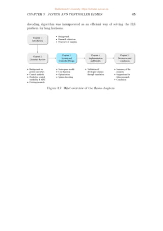
![Chapter 4
Implementation and Results
4.1 Introduction
In this chapter the current control strategy developed in Chapter 3 is evaluated
in terms of its applicability to grid-tied converters by comparing the following
approaches through simulation:
• model predictive control (MPC) with a short prediction horison of one
time step,
• model predictive control with a long prediction horison of twelve time
steps,
• open-loop pulse width modulation (PWM), a general technology that is
used with grid-connecting power converters [18], and
• naturally-sampled space vector modulation (SVM), a variation of PWM.
Firstly the simulation design provides an explanation on how these control
scenarios are implemented in simulation to allow for their evaluation.
Thereafter the results produced by the simulation are presented and discussed.
Finally the conclusion provides a summary of the findings.
4.2 Simulation design
4.2.1 Model predictive control
A MATLAB script was written to simulate the controller that is discussed in
Chapter 3. In Figure 4.1 a flow diagramme is presented which explains the
logic processes within the written MATLAB script. The first task is to initialise
the system parameters such as the filter’s component values, and provide the
state-space matrices that describe the system behaviour. These are then used
to build the integer quadratic formulation matrices Γ, Υ, Ψ, S and E. The
46
Stellenbosch University https://scholar.sun.ac.za](https://image.slidesharecdn.com/geldenhuysmodel20418-220210175802/85/Geldenhuys-model-20418-63-320.jpg)
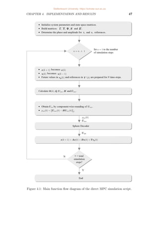
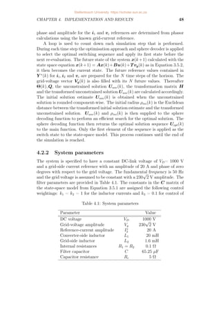
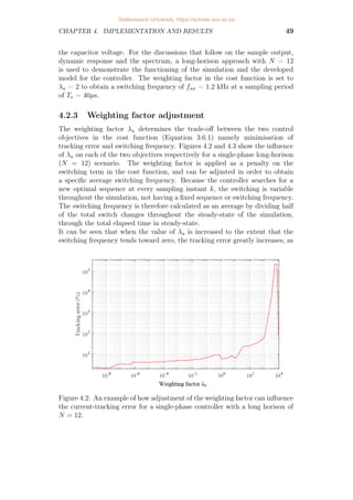
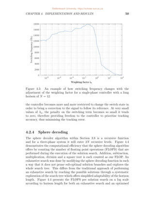
![CHAPTER 4. IMPLEMENTATION AND RESULTS 51
Figure 4.4: FLOPS executed during an exhaustive search, and during an
optimised search using sphere decoding.
search completed by the sphere decoder. The FLOPS are counted for each
time step of the first fundamental period from t = 0s to t = 0.02s and then
averaged. It can be seen that an exhaustive search becomes computationally
overwhelming [12] at a horison length of about N = 8, but it indicates a definite
trend for what can be expected from the longer horisons. Both the exhaustive
and sphere decoding methods display exponential growth as the horison length
increases. The sphere decoding algorithm provides a very significant reduction
in computational effort and is able to allow predictions of up to fifteen time
steps long.
4.2.5 Disregarding the grid
The MPC strategy developed incorporates the grid voltage in the optimisation
approach building on previous work done [46]. To determine the performance
of a controller that does not consider the grid voltage, the grid voltage vector
Vg = [vg(k) vg(k + 1) . . . vg(k + N − 1)] is set to zero for the solution search.
When calculating the outcome of the state variables as a result of the selected
switching action, the grid-voltage is given its true value to determine the effect
in a grid-connected scenario. Figure 4.5 provides the resulting grid-side current
waveform i2a and the reference signal i∗
2a. It is seen that the controller is unable
to provide accurate current tracking with the amplitude of i2a about a quarter
of that of its reference.
Stellenbosch University https://scholar.sun.ac.za](https://image.slidesharecdn.com/geldenhuysmodel20418-220210175802/85/Geldenhuys-model-20418-68-320.jpg)
![CHAPTER 4. IMPLEMENTATION AND RESULTS 52
Figure 4.5: Resulting grid-side current and reference for a controller that
disregards the grid-voltage in the optimisation approach.
4.2.6 Sample output
Figure 4.6 provides the steady-state grid-side current i2 against its reference
i∗
2 in all three phases. It can be seen how the values of i2 vary around the
corresponding references as a result of the switching ripple. This variation
coincides with the changing switch states. It can be seen that the waveforms
are not identical. The switch state in a specific phase leg does have an influence
on the future states of the system across all phases. During the selection
of an optimal control sequence, the switching sequence within each phase
may differ in any way, as long as the resulting three-phase waveforms are
collectively most optimal according to the weighted objectives within the cost
function. Therefore the selected three-phase switching sequence must minimise
the cost J by providing the best trade-off between the number of switching
and reference-tracking error combined.
Figure 4.7 shows the two a-phase inductor currents i1a and i2a with their
references. A phase difference which is introduced by the filter capacitance
[47] is observed between the two inductor currents. The converter-side current
i1 is a result of large ripple. After this ripple current passes through the filter
capacitor, the ripple in the grid-side current i2 is greatly reduced compared
to that in i1. The a-phase capacitor voltage and its reference are provided in
Figure 4.8. The capacitor voltage is very smooth and follows its reference very
well without noticeable ripple.
Stellenbosch University https://scholar.sun.ac.za](https://image.slidesharecdn.com/geldenhuysmodel20418-220210175802/85/Geldenhuys-model-20418-69-320.jpg)
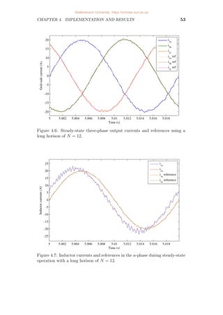
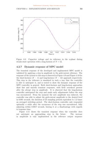
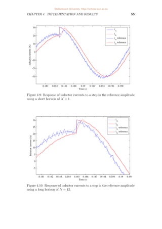
![CHAPTER 4. IMPLEMENTATION AND RESULTS 56
Figure 4.11: Response of inductor currents to an unanticipated step in the
reference amplitude using a long horison of N = 12.
Y ∗
(k) = [y∗
(k + 1) . . . y∗
(k + N)]T
once the step reaches time step k.
The long-horison controller has minimal overshoot and is also able to adjust
quickly within 0.001 seconds, but is not able to minimise the tracking error as
effectively as an anticipated step where the controller implements adjustments
before the step is reached.
4.3 Spectral analysis of MPC
Figure 4.12 provides the resulting spectrum I2(f) in decibels (dB) for a
long-horison approach with N=12, fsw=1.2 kHz and Ts=40µs calculated
from the grid-side current’s values between 250 and 350 simulated periodic
50 Hz cycles using a rectangular window. Model predictive control spreads
the spectral content by transferring some of the switching energy into noise
instead of harmonics. For this reason the spectrum is divided up into 50 Hz
frequency bands which serve as bins within which all energy is summed to
produce the discrete harmonics that take into account all energy, including
that dispersed as noise. The resulting harmonics of I2(f) and I1(f), at
multiples of the fundamental 50 Hz frequency, are provided in Figure 4.13 and
Figure 4.14 respectively. The first harmonic is at the fundamental frequency
f1 and represents the amplitude of the sinusoidal grid-side current i2 and
converter-side current i1. The harmonics that follow represent the distortion
in the signals.
Stellenbosch University https://scholar.sun.ac.za](https://image.slidesharecdn.com/geldenhuysmodel20418-220210175802/85/Geldenhuys-model-20418-73-320.jpg)
![CHAPTER 4. IMPLEMENTATION AND RESULTS 57
Figure 4.12: Output-current spectrum of the a-phase.
Figure 4.13: Output-current spectrum of the a-phase with discrete harmonics.
The total harmonic distortion (THD) of the grid-side current is calculated
by taking the square root of the sum of squared harmonic amplitudes excluding
the fundamental component I2(1), then dividing that square root by I2(1) [16;
80]. The overall THD for the three phases was determined by summing the
Stellenbosch University https://scholar.sun.ac.za](https://image.slidesharecdn.com/geldenhuysmodel20418-220210175802/85/Geldenhuys-model-20418-74-320.jpg)
![CHAPTER 4. IMPLEMENTATION AND RESULTS 58
Figure 4.14: Converter-current spectrum of the a-phase with discrete
harmonics.
THD’s of the individual phases and taking their mean [12].
THD =
1
I2(1)
v
u
u
t
∞
X
n=2](https://image.slidesharecdn.com/geldenhuysmodel20418-220210175802/85/Geldenhuys-model-20418-75-320.jpg)


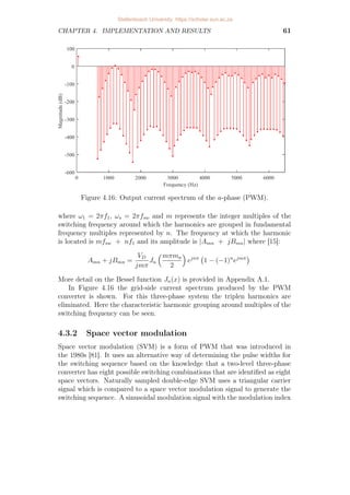
![2
× 100%
4.3.1 Pulse width modulation
The direct MPC current-control model developed during this study is
compared to the performance of an open-loop, naturally sampled PWM control
scheme. Pulse width modulation (PWM) is studied extensively as a classic
method for current control. The comparator of a pulse width modulator
generates a pulsed signal by comparing a sinusoidal reference voltage to a
triangular carrier signal. This pulsed signal drives the semiconductor switches
and has a fundamental component that is proportional to the reference
signal [10]. To implement the PWM controller and obtain its resulting
grid-current spectrum, the amplitude and phase of the reference signal has to
be determined. Firstly the impedances in the system, provided in Figure 4.15,
are grouped as follows:
Stellenbosch University https://scholar.sun.ac.za](https://image.slidesharecdn.com/geldenhuysmodel20418-220210175802/85/Geldenhuys-model-20418-79-320.jpg)

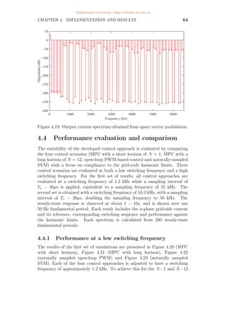
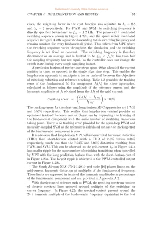
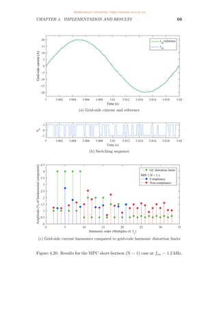
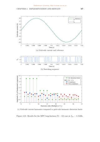
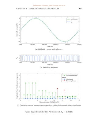
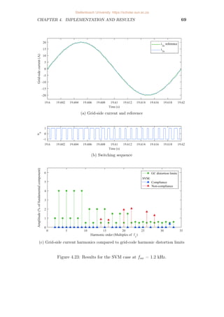
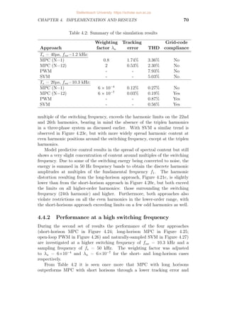
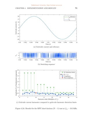
![.
The Fourier series expansion of the output voltage from the inverter can be
expressed as follows [15]:
vi(t) =
1
2
A00 +
∞
X
n=1
[A0n cos(nω1t) + B0n sin(nω1t)]
+
∞
X
m=1
[Am0 cos(mωst) + Bm0 sin(mωst)]
+
∞
X
m=1
±∞
X
n=±1
[Amn cos(mωst + nω1t) + Bmn sin(mωst + nω1t)] ,
Stellenbosch University https://scholar.sun.ac.za](https://image.slidesharecdn.com/geldenhuysmodel20418-220210175802/85/Geldenhuys-model-20418-89-320.jpg)
![CHAPTER 4. IMPLEMENTATION AND RESULTS 61
Figure 4.16: Output current spectrum of the a-phase (PWM).
where ω1 = 2πf1, ωs = 2πfsw and m represents the integer multiples of the
switching frequency around which the harmonics are grouped in fundamental
frequency multiples represented by n. The frequency at which the harmonic
is located is mfsw + nf1 and its amplitude is |Amn + jBmn| where [15]:
Amn + jBmn =
VD
jmπ
Jn
mπma
2
ejnπ
1 − (−1)n
ejmπ
More detail on the Bessel function Jn(x) is provided in Appendix A.1.
In Figure 4.16 the grid-side current spectrum produced by the PWM
converter is shown. For this three-phase system the triplen harmonics are
eliminated. Here the characteristic harmonic grouping around multiples of the
switching frequency can be seen.
4.3.2 Space vector modulation
Space vector modulation (SVM) is a form of PWM that was introduced in
the 1980s [81]. It uses an alternative way of determining the pulse widths for
the switching sequence based on the knowledge that a two-level three-phase
converter has eight possible switching combinations that are identified as eight
space vectors. Naturally sampled double-edge SVM uses a triangular carrier
signal which is compared to a space vector modulation signal to generate the
switching sequence. A sinusoidal modulation signal with the modulation index
Stellenbosch University https://scholar.sun.ac.za](https://image.slidesharecdn.com/geldenhuysmodel20418-220210175802/85/Geldenhuys-model-20418-90-320.jpg)
![CHAPTER 4. IMPLEMENTATION AND RESULTS 62
ma as amplitude and the modulation angle φ added to the phase:
i∗
abc = ma
sin(2πft + φ)
sin(2πft + φ − 2π
3
)
sin(2πft + φ − 4π
3
)
is modified to generate the space-vector equivalent modulation waveform [81]:
i∗
mod = i∗
abc −
1
2
(max(i∗
abc) + min(i∗
abc))
In Figure 4.17 the space-vector modulation waveform is compared to the
triangular carrier signal. For instance, intervals where the instantaneous value
of the modulation waveform is greater than the carrier signal, the switch state
is set to u = 1. In the opposite case the switch state becomes u = −1, as can
be seen in Figure 4.18.
Figure 4.17: Triangular carrier, space-vector modulation signal and sinusoidal
waveform generated to determine the switching pulse widths.
Figure 4.18: Space-vector modulated switching pulses.
Stellenbosch University https://scholar.sun.ac.za](https://image.slidesharecdn.com/geldenhuysmodel20418-220210175802/85/Geldenhuys-model-20418-91-320.jpg)
![CHAPTER 4. IMPLEMENTATION AND RESULTS 63
The frequency at which the harmonic is located is mfsw + nf1 and its
amplitude is |Amn + jBmn| where
A0n + jB0n|n1 =
√
3maVD
π
1
n + 1
sin
[n + 1]
π
6
cos
[n + 1]
π
2
×
n√
3 + 2 cos
[n + 1]
π
3
+
π
6
o
+
1
n − 1
sin
[n − 1]
π
6
cos
[n − 1]
π
2
×
n√
3 + 2 cos
[n − 1]
π
3
−
π
6
o
for the baseband harmonics (m = 0, n 1) [81]. More detail is provided on
the Bessel function Jn(x) in Appendix A.1. In the case of the carrier harmonics
(m 0, n = 0) and sideband harmonics (m 0, n 6= 0) the next equation is
used to determine the harmonic amplitudes [81]:
Amn + jBmn =
8VD
mπ2
π
6
sin
[m + n]
π
2
(
Jn
m
3π
4
ma
+ 2 cos n
π
6
Jn m
√
3π
4
ma
!)
+
1
n
sin m
π
2
cos n
π
2
sin n
π
6
(
J0
m
3π
4
ma
− J0 m
√
3π
4
ma
!)](https://image.slidesharecdn.com/geldenhuysmodel20418-220210175802/85/Geldenhuys-model-20418-92-320.jpg)
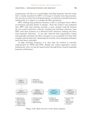

![n6=0
+
∞
X
k=1
k6=−n
1
[n + k]
sin
[m + k]
π
2
cos
[n + k]
π
2
sin
[n + k]
π
6
×
(
Jk
m
3π
4
ma
+ 2 cos
[2n + 3k]
π
6
Jk m
√
3π
4
ma
!)
+
∞
X
k=1
k6=n
1
[n − k]
sin
[m + k]
π
2
cos
[n − k]
π
2
sin
[n − k]
π
6
×
(
Jk
m
3π
4
ma
+ 2 cos
[2n − 3k]
π
6
Jk m
√
3π
4
ma
!)
Figure 4.19 provides the spectrum of the converter’s space-vector
modulated grid-side current. In three-phase systems the triplen harmonics are
eliminated. It can be seen that the harmonic content is concentrated around
multiples of the switching frequency, which is fsw = 1.2 kHz in this case.
Stellenbosch University https://scholar.sun.ac.za](https://image.slidesharecdn.com/geldenhuysmodel20418-220210175802/85/Geldenhuys-model-20418-96-320.jpg)
![CHAPTER 4. IMPLEMENTATION AND RESULTS 65
cases, the weighting factor in the cost function was adjusted to λu = 0.8
and λu = 2 respectively. For PWM and SVM the switching frequency is
directly specified beforehand as fsw = 1.2 kHz. The pulse-width modulated
switching sequence shown in Figure 4.22b, and the space vector modulated
sequence in Figure 4.23b is generated according to this switching frequency and
remains constant for every fundamental period. This differs from MPC where
the switching sequence varies throughout the simulation and the switching
frequency is not fixed or constant. The switching frequency is therefore
determined as an average and is limited to be fsw fs/2, less than half
the sampling frequency but not equal, as the controller does not change the
switch state during every single sampling instant.
A prediction horison of twelve time steps spans 480µs ahead of the current
position in time, as opposed to the single 40µs time step. This enables the
long-horison approach to anticipate a better trade-off between the objectives
of switching reduction and reference tracking. Table 4.2 provides the tracking
error of the fundamental 50 Hz component I2(f1) for these approaches,
calculated as follows using the amplitude of the reference current and the
harmonic amplitude at f1 obtained from the fft of the grid current:
tracking error =
I2(f1) − I2 ref
I2 ref
× 100%
The tracking errors for the short- and long-horison MPC approaches are 1.74%
and 0.53% respectively. This verifies that long-horison control provides an
optimised trade-off between control objectives by improving the tracking of
the fundamental component with the same number of switching transitions
taking place. There is no tracking error provided for the open-loop PWM and
naturally-sampled SVM as the reference is calculated so that the tracking error
of the fundamental component is zero.
It is also seen that long-horison MPC offers lower total harmonic distortion
(THD) than short-horison control with a THD of 2.3% versus 3.36%
respectively, much less than the 7.93% and 5.03% distortion resulting from
PWM and SVM. This can be observed as the grid-current i2a in Figure 4.21a
has smaller ripple for the same number of switching transitions when controlled
by MPC with the long prediction horison than with the short-horison control
in Figure 4.20a. The largest ripple is observed in the PWM-controlled output
current in Figure 4.22a.
The South African NRS 079-2-1:2010 grid code [16] places limits on the
grid-current harmonic distortion at multiples of the fundamental frequency.
These limits are expressed in terms of the harmonic amplitudes as percentages
of the fundamental component and are provided in Appendix A.2.
With classic control schemes such as PWM, the resulting spectrum consists
of discrete spectral lines grouped around multiples of the switching- or
carrier frequency. In Figure 4.22c the spectral content present around the
24th harmonic multiple of the fundamental frequency, equivalent to the first
Stellenbosch University https://scholar.sun.ac.za](https://image.slidesharecdn.com/geldenhuysmodel20418-220210175802/85/Geldenhuys-model-20418-98-320.jpg)
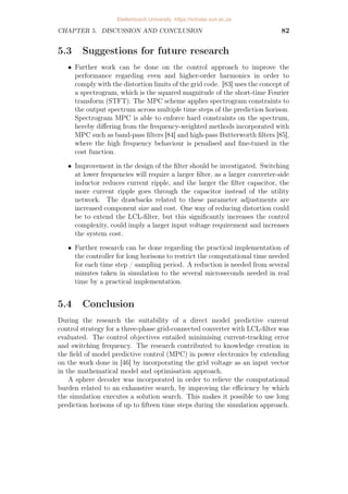


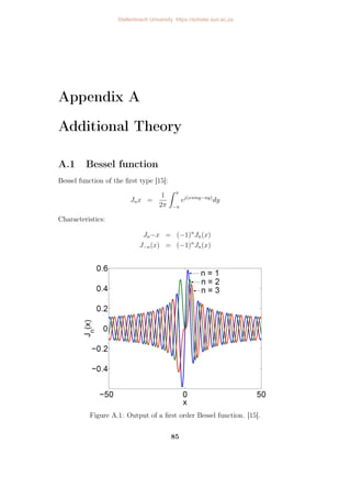


![CHAPTER 4. IMPLEMENTATION AND RESULTS 75
THD percentage. Both the tracking error and THD are much lower at a high
switching frequency than those obtained at the low switching frequency. The
grid-side currents for all four scenarios are smooth with no noticeable ripple.
MPC with long horisons, PWM and SVM manage to perform within the
grid-code current-distortion limits. The grid-current spectrum produced by
MPC with a short horison adheres to all harmonic limits, except at the
tenth harmonic (500 Hz). This coincides with the resonant frequencies of
the LCL-filter [14]:
fres1 =
1
2π
√
CL2
and fres2 =
1
2π
r
C
L1L2
L1 + L2
,
which delivers fres1 = 493 Hz and fres2 = 512 Hz when substituting the
filter’s component values, provided in Table 4.1, into the equations. Through
the application of a longer prediction horison the MPC controller manages
to displace enough energy away from the filter’s resonant frequencies at the
tenth harmonic to fully comply with the harmonic distortion limits. This
eliminates the need for active damping (AD) of filter resonance (e.g.: through
virtual resistance (VR)-based approaches [63; 82; 48; 47]) as required by linear
controllers which make use of classic control techniques.
4.5 Summary
Figure 4.28 provides a glance on how this chapter relates to those
that surround it. This chapter provides the evaluation of the
model-predictive direct current-control strategy developed in Chapter 3, for
a three-phase grid-connected converter with LCL-filter by implementation in
a MATLAB-based simulation for evaluation. A sphere decoding algorithm was
implemented as a computationally efficient solver for the solution search. The
model shows correct functioning as current controller, fast transient response
and good reference tracking of the fundamental 50 Hz component. The
suitability of the current-control scheme for a grid-connected converter setup
was investigated by comparing it with open-loop PWM, naturally-sampled
SVM, as well as the short- and long-horison application of the developed MPC
scheme. The spectrum of the grid-side current was tested against the harmonic
distortion limits of the NRS 079-2-1:2010 grid code for current injected into
the grid. The evaluation was performed at both a low and a high switching
frequency.
At low frequencies both MPC with short- and long-horison approaches show
non-compliance with the harmonic limits in the higher frequency range around
the switching frequency and onwards, as well as limits at even harmonics in
the lower frequency range. With an increase in switching frequency a point
is reached where the method manages to comply with the grid-code harmonic
Stellenbosch University https://scholar.sun.ac.za](https://image.slidesharecdn.com/geldenhuysmodel20418-220210175802/85/Geldenhuys-model-20418-108-320.jpg)
![Chapter 5
Discussion and Conclusion
In this chapter a summary is given of the whole thesis and how the research
objectives were met, where-after the main findings and recommendations for
future research are made before the final conclusion is drawn.
5.1 Summary of the research
The focus of the research is the development and evaluation of a MPC
current-control strategy for a three-phase grid-connected converter with
LCL-filter. All of the research objectives were achieved during the study:
• A discrete-time state space model was derived that describes the grid-tied
converter.
• The optimisation approach for MPC with long horisons as described in
[46] was adapted and extended to incorporate the grid voltage.
• The following control objectives were incorporated into the cost function:
– To minimise current tracking error.
– To minimise switching frequency.
• A sphere decoding algorithm was described and implemented as
a recursive function that solved the optimisation problem in a
computationally efficient manner.
• The developed control approach was implemented and evaluated by
MATLAB-based simulations.
A review follows on each chapter to summarise the main points that were
addressed in the thesis and how they support the objectives of the study.
77
Stellenbosch University https://scholar.sun.ac.za](https://image.slidesharecdn.com/geldenhuysmodel20418-220210175802/85/Geldenhuys-model-20418-110-320.jpg)
![CHAPTER 5. DISCUSSION AND CONCLUSION 78
5.1.1 Chapter 1
The first chapter introduced the background and context of the research, stated
the main focus and objectives of the thesis and provided a roadmap of the thesis
chapters.
5.1.2 Chapter 2
A literature review was conducted to provide an understanding of and
background on the history and applications of power converters. A
classification and discussion was provided on the types of control methods that
are applied to power converters, followed by a discussion on the suitability
of predictive control methods to present-day control systems and power
converters. The specific types of predictive control methods and specifically
model predictive control (MPC), its benefits, drawbacks and basic concepts,
were discussed. A review was done on existing research relevant to model
predictive control of grid-tied converters.
5.1.3 Chapter 3
In Chapter 3 the three-phase system and the proposed controller are described
and developed mathematically by defining the constraints of the finite control
set regarding the integer switch states, and deriving a state-space model that
can be used to describe and predict the behaviour of the system according to
its inputs, hereby achieving the first objective.
This model differs from that developed in [46] as within the state-space
equation the grid voltage is considered as an additional input vector alongside
the switch-state input vector, rather than being included in the state vector
as is the general trend in [47; 48]. This meant that the algebra of the standard
MPC optimisation approach be reworked to accommodate the inclusion of the
grid voltage as an input vector and this achieved the second objective of the
research.
For the third objective a cost function was formulated to include two
weighted control objectives, namely reducing reference tracking error and
secondly switching frequency reduction as a means to reduce losses in the
converter. This cost function was used to evaluate the optimality of available
switching actions, as the option that minimises the cost is the most optimal.
The state-space equation was used to predict the future behaviour of the
system according to a specific sequence of switching states applied. The
cost of each switch action was summed over the prediction horison of N time
steps to give the overall cost of a specific switching-sequence. The number of
possible sequences and their predicted outcomes increased exponentially the
longer the chosen horison length, posing an exhaustive search computationally
if every available sequence was to be evaluated. The minimisation of the
Stellenbosch University https://scholar.sun.ac.za](https://image.slidesharecdn.com/geldenhuysmodel20418-220210175802/85/Geldenhuys-model-20418-111-320.jpg)

![[9_CV] FCS-Model Predictive Control of Induction Motors feed by MultilLevel C...](https://cdn.slidesharecdn.com/ss_thumbnails/9cvfcs-modelpredictivecontrolofinductionmotorsfeedbymultillevelcasadedh-bridgeinverter-190418083950-thumbnail.jpg?width=640&height=640&fit=bounds)


