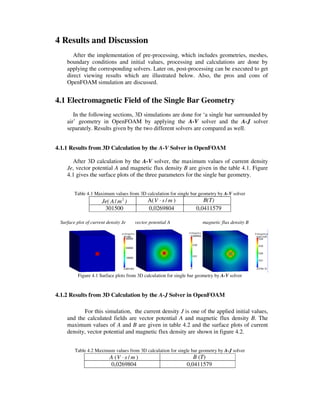
This thesis extends the electromagnetic field calculation capabilities of the open-source CFD software OpenFOAM. It develops new solvers within OpenFOAM to solve magnetostatic problems for materials like copper, steel, and permanent magnets. Two formulations (A-V and A-J) are derived from Maxwell's equations and implemented as OpenFOAM solvers through custom C++ code. Force calculation methods are also implemented to calculate Lorenz force and Maxwell stress. Simple test cases are modeled and solved to validate the new solvers. Results are compared to COMSOL Multiphysics and good agreement is found. The developed solvers could be applied to the design of electromagnetic devices like electric machines.

1. OpenFOAM Simulation for
Electromagnetic Problems
Zhe Huang
Master of Science Thesis in Electric Power Engineering
Department of Energy and Environment
Division of Electric Power Engineering
CHALMERS UNIVERSITY OF TECHNOLOGY
Göteborg, Sweden, 2010

2. September, 2010
Department of Energy and Environment
Chalmers University of Technology
SE-412 96 Gothenburg
Sweden
Telephone + 46 (0)31-772 1000
Cover:
[Simulation results from ANSYS software]
[Chalmers Reproservice]
Gothenburg, Sweden 2010
OpenFOAM Simulation for Electromagnetic Problems
Zhe Huang
Department of Energy and Environment
Chalmers University of Technology

3. SUMMARY
Simulation is considered as one of the most important and cost efficient approach of
industry research and development. OpenFOAM is one simulation tool with manual
solver compilation ability and 3D calculation capability, used for instance for
computational fluid dynamics (CFD) [1].
This thesis work is based on the OpenFOAM ‘rodFoamcase’ and the ‘rodFoam’ solver
used for plasma arc welding simulations which calculates the magnetic field in air. The
thesis work extends the case and the solver to solve electromagnetic field problems for
more materials including copper, linear steel and permanent magnets with different
geometries. In the future, this work can be applied into the design procedures of
electromagnetic devices, like electrical machines.
Based on the Maxwell equations, two different formulations (the A-V formulation and
the A-J formulation) are derived to solve magnetrostatic field problems. Formulations are
compiled manually into OpenFOAM solvers according to mathematic models by specific
program codes. Furthermore, force calculation equations are derived with the Lorenz
Force Method and the Maxwell Stress Tensor method. Then, simple geometries with
specific initial values and boundary conditions are calculated to test the new solvers.
The results of the developed simulation procedures in OpenFOAM are compared to the
results of another simulation software; COMSOL Multiphysics. It is found that the
simulation results show a very good agreement between OpenFOAM simulations and
COMSOL simulations.
Prediction of the future utilization of this thesis work and directions of development
are also discussed.
Keywords: OpenFOAM, electromagnetic field calculation, force calculation.

4. Contents
Symbols and Abbreviations .....................................................................6
1 Introduction ..........................................................................................7
2 Theoretical Background........................................................................8
2.1 Maxwell Equations..........................................................................................8
2.2 Derived Formulations for 3D Electromagnetic Field Problems ........................8
2.2.1 A-V formulations .........................................................................................9
2.2.2 A-J formulations......................................................................................... 10
2.2.3 Equations for Magnetostatic Field Problems with Permanent Magnets........ 10
2.2.4 Transient State Formulations for Electromagnetic Field Problem................ 10
2.3 Formulations for Force Calculations of 3D Problems..................................... 11
2.3.1 Lorenz Force Method ................................................................................. 11
2.3.2 Maxwell Stress Tensor ............................................................................... 11
2.4 Brief Overview of OpenFOAM ..................................................................... 12
2.4.1 Competitive Strength of OpenFOAM ......................................................... 12
2.4.2 File Structure of OpenFOAM Cases ........................................................... 13
2.4.3 Solvers Compilation ................................................................................... 14
3 Implementation in OpenFOAM ..........................................................16
3.1 Modelling Methods ....................................................................................... 16
3.2 Electromagnetic Field Calculation for a Single Bar Geometry ....................... 16
3.2.1 A-V Solver and A-J solver Comparison on a 3D Geometry ......................... 16
3.2.2 Comparison between OpenFOAM and COMSOL Simulations on a 2D Axis
Symmetric Geometry .......................................................................................... 21
3.3 Single Bar with Copper Ring Geometry......................................................... 24
3.3.1 Geometry Properties................................................................................... 24
3.3.2 Mesh Generation ........................................................................................ 24
3.3.3 Boundary Conditions and Initial Values...................................................... 25
3.3.4 Solver Compilation..................................................................................... 27
3.4 Single Bar with Copper Ring and Permanent Magnets Geometry .................. 28
3.4.1 Geometry Properties and Mesh Generation................................................. 28
3.4.2 Boundary Condition and Initial Values....................................................... 29
3.4.3 Solver Compilation..................................................................................... 29
3.5 Force Calculation for Two Parallel Current-Carrying Bars ............................ 30
3.5.1 Geometry Properties................................................................................... 30
3.5.2 Boundary Conditions and Initial Values...................................................... 31
3.5.3 Lorenz Force Solver Compilation............................................................... 31
3.5.4 Maxwell Stress Tensor Solver .................................................................... 32
4 Results and Discussion .......................................................................33
4.1 Electromagnetic Field of the Single Bar Geometry ........................................ 33
4.1.1 Results from 3D Calculation by the A-V Solver in OpenFOAM.................. 33
4.1.2 Results from 3D Calculation by the A-J Solver in OpenFOAM................... 33
4.1.3 OpenFOAM and COMSOL Simulation Comparisons on a 2D Axis ........... 34
Symmetric Geometry .......................................................................................... 34

5. 4.2 Simulation Results of Single Bar with Copper Ring Geometry ...................... 37
4.3 Simulation Results of the Single Bar with a Copper Ring and Permanent
Magnets .............................................................................................................. 37
4.4 Simulation Results Comparison of Force Calculation .................................... 39
4.4.1 Field Distribution Comparison between OpenFOAM and COMSOL.......... 39
4.4.2 Numerical Results of Lorenz Force Method and Maxwell Stress Tensor..... 40
Method................................................................................................................ 40
5 Conclusions and Future Work.............................................................42
Appendix 1 ............................................................................................44
Appendix 2 ............................................................................................48
Appendix 3 ............................................................................................50
Appendix 4 ............................................................................................52
Appendix 5 ............................................................................................53
References .............................................................................................54

6. Symbols and Abbreviations
⋅∇ divergence operator
×∇ curl operator
∇ gradient operator
t∂
∂ partial derivative
A magnetic vector potential msV /⋅
B magnetic flux density T
D electric displacement field 2
/ mC
E electric field intensity V/m
H magnetic field intensity A/m
CH coercive magnetic field of permanent magnets A/m
I current of conductor A
J current density 2
/ mA
L total length of conductor m
R resistance Ω
S total area of conductor 2
m
V electrical scalar potential V
ρ electric charge density 3
/ mC
ε permittivity F/m
µ magnetic permeability mAWb ⋅/
rµ relative magnetic permeability
0µ permeability in the free space
ν magnetic reluctivity
rν relative magnetic reluctivity
σ electrical conductivity S/m

7. 1 Introduction
Since ‘Energy Shortage’ and ‘Greenhouse Effect’ are two of the most severe
problems nowadays, energy efficiency and clean energy are becoming more and
more important. Further, simulation is considered as one of the most important and
cost efficient approach of industry research and development. OpenFOAM is one
simulation tool with manual solver compilation ability and 3D calculation capability,
used for instance for computational fluid dynamics (CFD) [1].
This thesis work aims at expanding the calculation range of OpenFOAM, by using
C++ syntax in OpenFOAM, in order to solve electromagnetic field problems, which
can be applied into the design procedures of electromagnetic devices, like electrical
machines. The work is one part of electromagnetic devices design performed by the
vehicle company Volvo, and will be one step towards reaching the goal of the
highest electrical efficiency in electrical machines.
In order to design the optimized geometry and predict the operation behaviour, an
accurate knowledge of the field quantities inside the magnetic circuit is necessary
[2]. OpenFOAM is a powerful calculation tools for obtaining complex PDE
solutions. It has its own superiority compared to other commercial software, which
is not only on its free-of-charge and open source licence, but also on its numerous
solvers, utilities and libraries [1]. Compared to the ‘black-box’ solvers in other
commercial softwares, new physics-mathematics models can be compiled into new
solvers based on these features of OpenFOAM.
With implemented methods of the finite element method (FEM), the finite volume
method (FVM) and the finite area method (FAM), OpenFOAM is the majority
investigated simulation software of this thesis work aimed to enlarge the calculation
range to calculate electromagnetic fields. Meanwhile, some of the OpenFOAM cases
are simulated in another commercial software COMSOL with the same initial field
values and boundary settings. This is done in order to check the validity of the edited
solvers with different mathematic models in the OpenFOAM simulations.
These new solvers can be applied into any electromagnetic devices such as an
electrical machine, in order to obtain the lowest cost and optimal design.
Chapter 2 describes different ways of formulating static electromagnetic field
problems according to Maxwell Equations. Based on the obtained electromagnetic
field, two electromagnetic force calculation methods are discussed. Besides, the
structure of OpenFOAM files is briefly illustrated.
Chapter 3 gives four practical examples of electromagnetic field and force
calculations by OpenFOAM. Each calculation contains the solver compilation and
pre-processing, which includes mesh generation, initial values and boundary
condition application, and post-processing.
Chapter 4 shows the results of all applications in chapter 3 and also discusses pros
and cons of OpenFOAM calculations.
Chapter 5 summarises the thesis work and predicts its future utilizations.
Meanwhile other interesting research trends about this topic are also discussed.

8. 2 Theoretical Background
2.1 Maxwell Equations
The complete set of Maxwell equations is shown as below:
t
D
JH
∂
∂
+=×∇ (2.1)
0=⋅∇ B (2.2)
t
B
E
∂
∂
−=×∇ (2.3)
ρ=⋅∇ D (2.4)
where H is the magnetic field intensity, J is the current density, D is the electric flux
density, B is the magnetic flux density, t is the time, E is the electric field intensity,
and ρ is the electric charge density. There is interdependency between all variables
in the equations and, therefore, a unique solution [3].
For stationary or quasi-stationary electromagnetic field distribution cases, the
displacement current density term
t
D
∂
∂
is neglected, which gives the equation as
below
JH =×∇ (2.5)
Since the divergence of the curl of any vector field in three dimensions is equal to
zero, the following equation is obtained
0)( =×∇⋅∇=⋅∇ HJ (2.6)
The macroscopic material properties are defined by the constitutive relations [3]:
ED ε= (2.7)
HHB r 0µµµ == (2.8)
EJ σ= (2.9)
where ε is the permittivity, µ is the magnetic permeability, rµ is the relative
permeability, 0µ is the permeability in free space and σ is the electrical
conductivity.
2.2 Derived Formulations for 3D Electromagnetic Field
Problems
There are several possible formulations used for electromagnetic field
calculations. This thesis work, which focuses on magnetostatic calculations of three-
dimensional field problems, are based on the magnetic vector potential A which is
defined by
BA =×∇ (2.10)

9. 2.2.1 A-V formulations
One type of the magnetic vector potential formulations is the A-V formulation
based on magnetic vector potential A coupled with the reduced electric scalar
potential V. V is defined in equation (2.11):
V
t
A
E ∇−
∂
∂
−= (2.11)
According to (2.10), the magnetic flux density B can be calculated if the magnetic
vector potential A is known. A is defined in the whole problem region. While for the
electric scalar potential V, at the two ends of conductor region, a high value of V and
a low value of V are defined separately. Also at the non-conducting region, the value
of V is zero. Further, the permeability is assumed constant in each material, thus
non-linearity of for instance electrical machine core parts are not considered.
For magnetostatic cases, the displacement magnetic vector potential term
t
A
∂
∂
is
neglected, which gives equation (2.12):
VE −∇= (2.12)
Combining (2.5) and (2.8) and (2.9) and (2.10) and (2.11), we will get
)(
)(
1
)(
VEJ
A
B
H
−∇===
×∇×∇=×∇=×∇
σσ
µµ (2.13)
which is equal to the equation
VA ∇−=×∇×∇ σ
µ
)(
1
(2.14)
By using the Coulomb Gauge [4],
0=⋅∇ A (2.15)
the A-V formulation in the static case will get the unique solution of A obtained as
below
0
11
=∇+





⋅∇∇−





×∇×∇ VAA σ
µµ
(2.16)
where the second term is a penalty term with the Coulomb gage. Due to the
addition of the Coulomb gauge, the solenoidality of the flux density must be
satisfied separately [4]. This is done by combining equations (2.6), (2.9) and (2.12)
into
0)( =∇−⋅∇ Vσ (2.17)
Equations (2.16) and (2.17) are compiled into an OpenFOAM solver and is applied
for the current-carrying single bar case, which will be further discussed in chapter 3.

10. 2.2.2 A-J formulations
Another type of formula used for static magnetic field calculations is the A-J
formulation which uses the electric current density J as driving force.
Combining (2.5) and (2.8) and (2.10), we will get
JA
B
H =×∇×∇=×∇=×∇ )(
1
)(
µµ
(2.18)
Using the Coulomb Gauge similar to (2.16), the A-J equation is descripted as
JAA =





⋅∇∇−





×∇×∇
µµ
11
(2.19)
Compared to the A-V formulation, the A-J formulation does not have V∇σ terms,
which means it is more time-saving when applying FEM or FVM in the calculation
softwares.
2.2.3 Equations for Magnetostatic Field Problems with Permanent Magnets
When different types of magnetic materials are utilized as driving source, the
magnetostatic equations below can be applied to calculate the electromagnetic fields,
where CH is the coercive magnetic field of permanent magnets.
0
11
=×∇−





⋅∇∇−





×∇×∇ CHAA
µµ
(2.20)[5]
This equation can be considered as a transition to equation (2.21) which will
calculate the fields generated by two driving sources including electric and magnetic
energy sources.
JHAA C =×∇−





⋅∇∇−





×∇×∇
µµ
11
(2.21)
2.2.4 Transient State Formulations for Electromagnetic Field Problem
Because of the time limitation of thesis work, transient equations of field
calculation are not used in this report. However, equation (2.22) shows the method
to calculate fields for transient electromagnetic problems, which can be helpful for
the continuing study.
0
11
=∇+
∂
∂
+×∇−





⋅∇∇−





×∇×∇ V
t
A
HAA C σσ
µµ
(2.22)[5]
As it is discussed before, due to the Coulomb Gauge [4] eqation (2.15), the
solenoidality of the flux density must be satisfied separately. If formulas (2.6), (2.9)
and (2.11) are combined, equation (2.23) will be obtained.
0=





∇−
∂
∂
⋅∇ V
t
A
σσ (2.23)

11. 2.3 Formulations for Force Calculations of 3D Problems
From the solution of an electromagnetic field problem, the potential or field flux
values are calculated firstly. Furthermore, other important parameters, such as force
or torque acting on various parts of machines can be obtained from the calculated
potential values. Four force or torque calculation methods are mostly used in finite
element analysis [6]:
(1) Lorenz Force Method
(2) Maxwell Stress Tensor Method
(3) Virtual Work Method
(4) Equivalent Source method
In this thesis work, the Lorenz Force method and the Maxwell Stress Tensor
method formulas have been investigated and applied into OpenFOAM in order to
calculate electromagnetic force, which are discussed in the following parts.
2.3.1 Lorenz Force Method
The Lorenz Force method can calculate the total force on a current-carrying
conductor by volume integration of the force density acting on each differential
current-carrying element. The Lorenz force can be calculated by
dVBJF V )( ×∫= (2.24)
where BJ × is the force density of the conductor.
By this method, the total current density J is necessary for the force calculation,
which means that this method is relatively easy to get numerical results of coil
forces of electrical machines. In contrast, it cannot determine the force acting on
ferromagnetic materials [7].
2.3.2 Maxwell Stress Tensor
The Maxwell Stress Tensor method can calculate force acting on a body by
integrating force density over a surface enclosing the body. The expression of the
Maxwell Stress Tensor is [6]:
)
2
1
(
1 2
ijjiij BBBT δ
µ
−=
(2.25)
where i and j can be replaced by (x, y, z) , 1=ijδ when i=j and 0=ijδ when i≠ j.
Therefore the Maxwell Stress Tensor can be expressed in another way as (2.26)
[6]:

12. [ ] [ ]
[ ] [ ]
[ ] [ ]
























−






−






−
=










=
22
22
22
2
1
)(
111
1
2
1
)(
11
11
2
1
)(
1
BBBBBB
BBBBBB
BBBBBB
TTT
TTT
TTT
T
zyzxz
zyyxy
zxyxx
zzzyzx
yzyyyx
xzxyxx
µµµ
µµµ
µµµ
(2.26)
The force calculation formula in terms of the force density vector is given by
TdSdSnBnBBF SS ∫=−⋅∫= )
2
1
)(
1
( 2
µµ
(2.27)[6]
where n is the normal unit vector to the surface under consideration.
Compared to the Lorenz Force method, the Maxwell Stress Tensor method is
more accurate, because this surface integral is not affected by the current density
distribution within the object but only by the accuracy of calculated magnetic field
density [7]. And this method can be applied to calculate electromagnetic force not
only for current source materials but also for ferromagnetic materials. Besides, the
integrating surface does not need to be the physical surface of the object, which can
be arbitrarily chosen but must be entirely placed in air. Further comparison between
the two different force calculation methods is given in chapter 4.
2.4 Brief Overview of OpenFOAM
2.4.1 Competitive Strength of OpenFOAM
OpenFOAM is a C++ based toolbox with revisable solvers to calculate partial
differential equations (PDE) and to simulate multi-physics problems, including
computational fluid dynamics (CFD). OpenFOAM includes a standard library and
great range of solvers, which shows as below [8]:
• Basic CFD
• Incompressible flows
• Compressible flows
• Multiphase flows
• Direct numerical simulations (DNS) and large eddy simulations (LES)
• Combustion
• Heat transfer and buoyancy-driven flows
• Particle-tracking flows
• Molecular dynamics
• Direct simulation Monte Carlo
• Electromagnetics
• Stress analysis of solids
• Finance
This thesis work is focused on extending the ‘Electromagnetics’ solver by using
C++ syntax in OpenFOAM.

13. In order to accomplish one simulation, two branches of files are needed in
OpenFOAM. One branch of files which is called ‘case file’ is used to illustrate
specific pre-processing, such as geometry, boundary conditions, initiate fields
setting and calculation steps and time and so on. The other branch of files which is
called ‘solver file’ includes the mathematic model and solution of a certain physic or
chemical or economic problem. In 2.4.2, the structures of OpenFOAM cases are
shortly introduced. In 2.4.3, the easy and quick equation editing method of
OpenFOAM is further described.
Besides, OpenFOAM is also supplied with mesh generator tools, such as
blockMesh, extrudeMesh, etc. Meanwhile, it accepts meshes generated by any of the
major mesh generators and CAD systems such as ANSYS mesh, CFX 4 mesh,
Fluent mesh, etc.
Furthermore, paraFoam, a reader module for OpenFOAM data for the open source
visualization application ParaView makes the post-processing of OpenFOAM
convenient and user-friendly.
Another reason of simulating in OpenFOAM is its availability of parallel
computing, which shows the great potential and opportunity for solving increasingly
complex problems.
2.4.2 File Structure of OpenFOAM Cases
The basic directory structure of an OpenFOAM case, which contains the
minimum set of files required to run an application, is shown in figure 2.1 [8]:
Figure 2.1 Directory structure of an OpenFOAM case
Case
System
Constant
ControlDict
fvSchemes
fvSolution
xProperties
Time directories
polyMesh
blockMeshDict
points
cells
faces
boundary

14. A ‘system’ directory defines simulation time and calculation algorithms.
Meanwhile, it can be used to define different inner fields by using specific utilities,
such as ‘setFieldDict’ and ‘funkySetFieldDict’. ‘funkySetFieldDict’ utility is
explained in chapter 3 when it is applied into simulation.
A ‘constant’ directory is used to describe the geometry and mesh case in the
subdirectory ‘polyMesh’, and specific physical properties (‘xProperties’) for a
certain case.
The ‘time’ directories contain different data files of particular fields for a case.
Different subdirectories with the name of numbers, which stands for different
calculation time steps are included. The ‘0’ directory contains the data files of
initialized field values.
The specific functions of each file will be illustrated more detailed in chapter 3.
2.4.3 Solvers Compilation
While OpenFOAM can be used as a standard simulation package, it is also
possible to look deep into the ‘black box’ to edit or program different partial
differential equations (PDE) by using the finite volume method (FVM) or the finite
element method (FEM) or the finite area method (FAM).
As other C++ programming codes, every piece of the original code in the
OpenFOAM solvers has to be organised by a standard structure in order to access
dependent components of the OpenFOAM library. The top level source file with the
.C extension, together with other source files, can be compiled by using the
command ‘wmake’, which is included in the directory ‘Make/files’. Figure 2.2
shows the basic directory structure of an OpenFOAM solver [8]:
Figure 2.2 Directory structure of an OpenFOAM solver
In OpenFOAM, there is a top-level code which is applied in the .C file and can
represent PDEs directly and flexibly.
For example, if the governing equation is given as equation (2.11):
V
t
A
E ∇−
∂
∂
−= (2.11)
OpenFOAM will represent this equation in its natural language:
solve ( E = = -fvm::ddt(A)-fvm::div(V))
newSolver
newSolver.C
otherHeader.H
Make
files
options

15. where fvm stands for Finite Volume Method and returns an fvMatrix, fvc stands
for Finite Volume Calculus and returns a geometricField.
Table 2.1 shows some of the correspondence between the mathematic expression
and the OpenFOAM expression [8]:
Table 2.1 Correspondence between mathematic expression and OpenFOAM expression [8]
Term
description
Mathematical expression fvm::/fvc:: functions
Laplacian φ∇Γ⋅∇ laplacian(Gamma,phi)
φ2
∇ laplacian(phi)
Time derivative t∂∂ /φ ddt(phi)
Gradient φ∇ grad(phi)
Divergence )(ϕ⋅∇ div(psi)
Curl φ×∇ curl(phi)
The application of these clear structures of ‘case’ and ‘solver’ is further
discussed in chapter 3.

16. 3. Implementation in OpenFOAM
3.1 Modelling Methods
With the implemented methods of the finite element method (FEM), the finite
volume method (FVM) and the finite area method (FAM), OpenFOAM is the
majority investigated simulation software of this thesis work used to calculate
electromagnetic fields. Meanwhile, some of the OpenFOAM cases are simulated in
another commercial software; COMSOL with the same initial field values and
boundary settings, in order to check the validity of the edited OpenFOAM solvers.
This thesis work is based on the OpenFOAM ‘rodFoamcase’ and the ‘rodFoam’
solver used for plasma arc welding simulations which calculates the magnetic field
in air. The thesis work extends the case and the solver to solve the electromagnetic
field problems for more materials including copper, linear steel and permanent
magnets with different geometries.
3.2 Electromagnetic Field Calculation for a Single Bar
Geometry
Simulation results from problems with the same 3D geometry and initial values
are compared of both A-V and A-J solvers. Another comparison is taken between
OpenFOAM and COMSOL on the 2D axis symmetric geometry in order to check
the calculation accuracy of the new OpenFOAM solvers. The problem used for the
comparisons consists of a single copper bar, surrounded by air, as described further
below.
3.2.1 A-V Solver and A-J solver Comparison on a 3D Geometry
(1)Geometry Properties
The problem is defined as follows:
Solution domain:
The calculated domain is a cuboid copper wire surrounded by a cuboid air box in
3 dimensions. The geometry data in 3D is given in table 3.1 and figure 3.1 shows the
problem region. For the SingleBarCase3D1, high voltage and low voltage are
applied to the two ends of the copper bar separately. For the SingleBarCase3D2,
current density J is applied to the copper bar. Magnetic fields are calculated for both
cases.
Table 3.1 Dimension of single bar geometry
x(m) y(m) z(m)
Conductor 0.4 0,4 6
Air box 4 4 6

17. Figure 3.1 Geometry of the single bar case
Solver name:
SingleBarFoam1 (with A-V solver)
SingleBarFoam2 (with A-J solver)
Case name:
SingleBarCase3D1 (with A-V solver)
SingleBarCase3D2 (with A-J solver)
(2) Mesh Generation
Figure 3.2 shows patches and points defined on the x-y plane (when z=0).
Numbers without circles represent different points and numbers with circles
represent different patches. The number 0 patch in the middle of the surface
represents the cuboid current-carrying cable.
67
238 11
9 0 1 10
54 12 13
1415
1
234
5
6 7 8
0
z x
y
Figure 3.2 Patches and points defined on the x-y plane (z=0)
x
y
leftleft
right
front
back
up
down

18. Generally, there are four validity constraints used in OpenFOAM: points, faces,
cells and boundary faces. These are basic constraints that a mesh must satisfy. As it
is shown in the figure 3.2, 16 points and 9 faces are defined for the front surface on
the x-y plane (z=0). For the whole 3 dimensional geometry, the length along the z-
direction is 6 m. Furthermore, the whole length along the z direction is divided into
10 units.
The OpenFOAM ‘BlockMesh’ utility is used to generate meshes in the file
constant /polyMesh/ blockMeshDict of the ‘case’directory. Inside this file, cell shape
and mesh density can be defined. Hexahedral, wedge, pyramid, tetrahedron, and
tetrahedral wedge cell shapes can be defined by ordering of point labels in
accordance with the numbering scheme contained in the shape model. Hexahedral
cell shape is used in this thesis work. One example of geometry definition is given in
the codes below [8]:
8 //declare the total number of points
(
(0 0 0) //point 0
(1 0 0) //point 1
(1 1 0) //point 2
(0 1 0) //point 3
(0 0 0.5) //point 4
(1 0 0.5) //point 5
(1 1 0.5) //point 6
(0 1 0.5) //point 7
A hexahedral block with 101010 ×× mesh density in OpenFOAM is written as:
hex (0 1 2 3 4 5 6 7) (10 10 10) simpleGrading (1 1 1)
The same geometry definition approach is applied to obtain more complex
geometry in this thesis work. The comprehensive mesh generation codes of this
geometry are given in Appendix 1, which has 400 cells in total.
Besides, the file boundary in the constant /polyMesh directory is used to define
type and total number of cells for each patch.
(3) Boundary Condition and Initial Fields for the 3D Geometry Cases
Boundary types are defined in the OpenFOAM file constant /polyMesh
/boundary. There are three attributes associated with a patch; the basic type, the
primitive type and the derived type. The ‘basic type’ is the one that has been used
most often in this thesis work and the different types of basic patches are shown in
table 3.2:

19. Table 3.2 Basic patch types in OpenFOAM
Name Description
Patch generic patch
symmetryPlane plane of symmetry
Empty front and back planes of a 2D geometry
Wedge wedge front and back for an axi-symmmetric geometry
Cyclic cyclic plane
Wall wall—used for wall functions in turbulent flows
For the 3D single bar problem,, ‘patch’ is used for every boundary. The boundary
type ‘wedge’ and ‘empty’ are used for the 2D axis symmetric cases later on. One
example of ‘boundary’ file is given in Appendix 2.
Field initial values of the boundaries are defined in the so called ‘0’ directory. For
the cases using the A-V formulation, the magnetic vector potential A, the electrical
scalar potential V and the electrical conductivity σ are pre-defined in the ‘0’
directory. Consequently, for the cases using the A-J formulation, the magnetic
vector potential A and the current density J are pre-defined in the ‘0’ directory. The
field initial values which need to apply in the inner region of geometries, such as
electrical conductivity σ in the cases which use the A-V solver and current density J
in the cases which use the A-J solver cases, are defined in file system/setFieldDict.
Table 3.3 shows the boundary conditions and initial values of the single bar 3D
problem when using the A-V formulation. The naming of boundaries are shown in
Fig. 3.1.
Table 3.3 Boundary conditions and initial values of the Single Bar 3D problem when using the A-V
formulation
Boundary names
(see Fig. 3.1)
A σ metalair µµ ≈ V
Air left and right
and back and
front
Fixed value 0 Fixed value 1e-
5
1.26e-6 Zero gradient
Air up and down Zero gradient Fixed value 1e-
5
1.26e-6 Zero gradient
Conductor up Zero gradient Fixed value
2700
1.26e-6 670 V
Conductor down Zero gradient Fixed value
2700
1.26e-6 0 V
Regarding figure 3.1, the left, right, back and front patches of the air box should
be infinitely far from the cable where the magnetic vector potential A is set to 0. The
boundary condition “zero gradient” represents that the normal gradient of the field is
zero. Since the values of the electrical conductivity are almost zero in air but quite
large in metal, 1e-5 S/m is chosen to represent air and 2700 S/m for the metallic
material. Furthermore, since the magnetic permeability µ of air in some cases is
almost equal to the value of metal, such as copper, 1.26e-6 mAWb ⋅/ is chosen in
this simulation.

20. In order to have the same driving force with the A-J formulation as it is using the
A-V formulation (which applies 670V) a current density of 2
/310500 mA is applied,
according to the calculation below:
σσ
L
J
S
L
IRIU ⋅=
⋅
⋅=⋅=
i.e.
2
/301500
6
2700670
mA
L
U
J =
⋅
=
⋅
=
σ
where U is the voltage of the conductor, I is the current of the conductor, L is the
total length of the conductor, and S is the total area of the conductor.
Table 3.4 shows the boundary condition and initial values of the single bar 3D
simulation when the A-J formulation is applied.
Table 3.4 Boundary condition and initial values of the single bar 3D problem when
using the A-J formulation
A copperair µµ ≈ J
Air left and right and
back and front
Fixed value 0 1.26e-6 Zero gradient
Air up and down Zero gradient 1.26e-6 Zero gradient
Conductor up Zero gradient 1.26e-6 Fixed value
(0,0,301500)
Conductor down Zero gradient 1.26e-6 Fixed value
(0,0,301500)
Appendix 3 gives an example of an initial field setting file ‘A’ in the ‘0’
directory. Further, Appendix 4 shows the inner field setting method of the current
density J.
(4)Solver Compilation and Calculation
As it is shown in chapter 2, the A-V formulation in the magneto static case is
given as in (2.16) and (2.17) where (2.16) is repeated below:
0
11
=∇+





⋅∇∇−





×∇×∇ VAA σ
µµ
(2.16)
The A-J formulation in the magneto static case is given as the following:
JAA =





⋅∇∇−





×∇×∇
µµ
11
(2.19)
Since
( ) ( ) FFF 2
∇−⋅∇∇=×∇×∇ (3.1)
the A-V formulation and the A-J formulation can be transformed into formula (3.2)
and (3.3):

21. 0
1 2
=∇+∇− VA σ
µ
(3.2)
JA =∇− 21
µ
(3.3)
Together with equation (2.17), these partial differential equations can be
expressed by the following OpenFOAM codes:
(a) A-V Solver equations
solve ( fvm::laplacian(sigma, ElPot) );
solve ( fvm::laplacian(A)==sigma*muMag*(fvc::grad(ElPot)) );
B= fvc::curl(A);
Je=-sigma*(fvc::grad(ElPot));
(b) A-J Solver equations
solve ( fvm::laplacian(A)==-muMag*J);
B= fvc::curl(A);
where muMag is the permeability (of air and the copper conductor).
Appendix 5 gives an example of the .C file of the A-J solver. This .C file
combined with the files in the ‘Make’ directory (refer to figure 2.2) can be compiled
by the ‘wmake’ command. After compilation, an executable file of the new solver is
generated. The executable file should be copied into the ‘Case’ directory and it is
used for calculations with specific boundary conditions and initial values.
(5)Post-processing
Post-processing is executed by the command ‘paraFoam’ which will call the
‘paraView’ software which is the main post-processor of OpenFOAM. After
calculation, the maximum value of current density, magnetic vector potential and
magnetic field density are compared between the A-V solver and the A-J solver
which is further discussed in chapter 4.1.
3.2.2 Comparison between OpenFOAM and COMSOL Simulations on a 2D Axis
Symmetric Geometry
Chapter 4.1 will show great similarity of calculation results from the OpenFOAM
A-V solver and A-J solvers applied to the same 3D geometry. Hence, if OpenFOAM
calculation results from the A-V solver show similarity to COMSOL calculation
results from this simulation test, the validity of the A-J solver in the 2D axis-
symmetric case should also be proved.

22. OpenFOAM needs 3D control volumes even for the 2D cases. However, the patch
type ‘empty’ can be applied to generate 2D or even 1D geometries by specifying
special patches into empty in one dimension or in two dimensions. Meanwhile, the
patch type ‘wedge’ can be used to specify a geometry as a wedge with a small angle
and being one cell thick along the plane of symmetry to obtain a 2D axi-symmetric
geometry, which is applied in the simulation below.
(1) Geometry properties for 2D axi-symmetric simulation applied in
OpenFOAM and COMSOL
2D axi-symmetric simulations are done both in OpenFOAM and COMSOL to
calculate electromagnetic fields of a cylindrical conductor placed in a cylindrical air
box. The 2D axi-symmetric geometry is shown in the right figure of figure 3.3 and
the geometry data is shown in table 3.5, where R is the radius of the cylindrical air
box, r is the radius of the cylindrical conductor, and L is the total length of the
geometry.
Figure 3.3 Geometry from 3D to 2D axis symmetric
Table 3.5 Data of 2D axis symmetric geometry
r(inner)(m) R(outer)(m) L(m)
0.2 2 6
x
L
R
y
r
Symmetry Axis
R
Air box
Cylindrical
conductor

23. (2) Mesh Generation
In OpenFOAM, the square meshes are still applied in the 2D axis symmetric
geometry; 10 cells are applied on the x direction and 30 cells are applied on the y
direction. Meanwhile, 1 cell unit is applied along the z direction to express the 2D
geometry. In COMSOL, the mesh generation is done by the default mesh type
‘Normal’.
(3) Boundary Condition and Initial Field
As shown in table 3.6 and table 3.7, the current density is used as the driving force
in COMSOL and the equivalent voltage is applied for the A-V solver in
OpenFOAM. In COMSOL, the current density is set to 0.3 2
/ mmA along y direction.
Consequently, in OpenFOAM, a voltage value of 670V is applied to the cylindrical
conductor, in order to introduce a current density of 0.3 2
/ mmA .
Table 3.6 Initial values for single bar simulation with 2D axis symmetric geometry in COMSOL
µ ( mH / ) J ( 2
/ mmA ) σ (S/m)
copper 1.26e-6 0.3 2700
air 1.26e-6 0 1e-5
Table 3.7 Initial values for single bar simulation with 2D axis symmetric geometry in OpenFOAM
µ ( mH / ) U(V) σ (S/m)
copper 1.26e-6 High: 670, Low: 0 2700
Air 1.26e-6 0 1e-5
There is one difference between OpenFOAM and COMSOL when they are used
for 2D axis symmetric simulation. In COMSOL, when 2D simulation is taken, 2D
geometry is drawn at the first place. In OpenFOAM, though 2D simulation is needed
to be done, 3D geometry is always needed to be drawn first. Then 2D axis
symmetric simulation is needed, the boundary conditions of two surfaces which are
parallel to the rotating axis are treated as type ‘wedge’. Table 3.8 shows the
boundary conditions applied in this single bar 2D axis symmetric simulation.
Table 3.8 Boundary conditions for single bar simulation with 2D axis symmetric geometry in
OpenFOAM
A( msV /⋅ ) U(V)
Air up and down and
back and front
Fixed value 0 Zero gradient
Air left and right Wedge Wedge
Copper bar up Zero gradient Fixed value 670
Copper bar down Zero gradient Fixed value 0
The simulation results from both soft-wares are discussed in chapter 4.1.

24. 3.3 Single Bar with Copper Ring
In this simulation, three different materials; a copper ring conductor, a steel bar
and air, are involved. As it is shown in figure 3.4 below, the cuboid steel bar is put
in the middle of the copper ring conductor.
Figure 3.4 Geometry of a steel cuboid bar with a ring-shape copper conductor
3.3.1 Geometry Properties
The geometry data of a steel cuboid bar with a ring-shape copper conductor is
shown as the table 3.9 below.
Table 3.9 Geometry data table of single bar with copper ring case
x(m) y(m) z(m)
Air Box 4 4 6
Steel Bar 0.14 0.14 3
Inner R Outer R Z
Copper Ring 0.2 0.21 1
3.3.2 Mesh Generation
The mesh on x-y plate, for the simulation with one copper conductor and one
cuboid steel bar, is generated as it is shown in figure 3.5.
z
x
y
up
down
front
back
left
right
air box
steel bar
copper conductor

25. Figure 3.5 Patches and points definition in the x-y plane
As it is shown in figure 3.5 of the ‘up surface’ in the x-y plane, 41 points are
defined. For the whole 3D geometry, 82 points and 35 blocks are defined to
illustrate the steel bar rounded by the copper tube which is surrounded by air. The
mesh definition approach is similar to the approach applied in the single bar case.
3.3.3 Boundary Conditions and Initial Values
The current density, J, in the ring shaped coil (with a magnitude of unity) can
be expressed as below:




=
++
−
0,, 2222
yx
x
yx
y
J
In order to set the coil different permeability values, the ‘funkySetField’ utility is
used. Compared to the utilization of the utility setFieldDict used in previous cases,
this utility can set non-uniform field values and non-uniform field application regions
by C++ commands whereas the utility setFieldDict can only set uniform fields. The
OpenFOAM C++ commands used instead of the mathematic expressions to set the
fields are given in the text below. The commands are put in the file
system/funkySetFieldsDict.
0 1
2
34
5
6
78
9
10
11
12
13
1516
17
18
19
20
2122
23
25 2624
27
28
29
30
31
3233
34
35 36 37
38 40 39
14
x
y

26. currentdensity2
{
field J; //field initialise
expression “vector( -301500*pos().y/sqrt(pow(pos().x,2)+pow(pos().y,2)),
301500*pos().x/sqrt(pow(pos().x,2) +pow(pos().y,2)), 0)”; //ring-shaped current
condition “sqrt(pow(pos().x,2)+pow(pos().y,2))>=0.2 &&
sqrt(pow(pos().x,2)+pow(pos().y,2))<=0.21 && pos().z>=3 && pos().z<=4”;
keepPatches 1;
dimensions [0 -2 0 0 0 1 0];
}
In the code above, ‘field’ is used to declare one field, ‘expression’ is used to write
field values, ‘condition’ will select a subset of the cells, and ‘dimensions’ describes
the dimension of the field in SI units.
In this simulation, the relative permeability is assumed to be constant (thus
saturation effects are ignored), and relative reluctivity can be expressed as in
formula (3.4),
µµµ
νν
11
0
0 =
⋅
=⋅
r
r (3.4)
where 0ν is the reluctivity of air, rν is the relative reluctivity of other materials, 0µ
is the permeability of air and rµ is the relative permeability of other materials.
The ‘funkySetField’ utility is used to express different permeabilities for different
regions in the following simulations. In the ‘funkySetField’ utility, one parameter,
such as permeability (or reluctivity), can be assigned with different values in
different volumes by changing the commands ‘expression’ and ‘condition’. The
field values are assigned by command ‘expression’, and the regions applying the
corresponding field values are declared by command ‘condition’. Besides, the latter
applied field value will overlap the previous field value for the same region.
Different relative permeabilities (or reluctivities) are defined by the command below
in the ‘funkySetFieldDict’ file.
relativereluctivity2 //copper ring
{
field viR; //field to initialise
expression “1”; //relative reluctivity in ring
condition “sqrt(pow(pos().x,2)+pow(pos().y,2))>=0.2 &&
sqrt(pow(pos().x,2)+pow(pos().y,2))<=0.21 && pos().z>=3 && pos().z<=4”;
keepPatches 1;
dimensions [0 0 0 0 0 0 0];
}

27. relativereluctivity3 //cuboid bar
{
field viR; //field initialise
expression “0.0005”; //relative reluctivity in bar
condition “pos().x>=-0.14 && pos().x<=0.14 && pos().y>=-0.14 &&
pos().y<=0.14 && pos().z>=2 && pos().z<=5”;
keepPatches 1;
dimensions [0 0 0 0 0 0 0];
}
In order to show the permeability difference between the coil and the steel, a high
permeability value (2000) is chosen for the steel bar. Table 3.10.1 and table 3.10.2
show the initial values and boundary conditions after executing funkySetField utility.
Table 3.10.1 Initial values for a copper coil with steel bar geometry:
J( 2
/ mA )(absolute value) rµ ( rν )
Air 0 1 (1)
Coil 301500 1 (1)
Steel bar 0 2000 (0.0005 )
Table 3.10.2 Boundary conditions for a copper coil with steel bar geometry:
A( msV /⋅ ) J( 2
/ mA )
Air left and right and
back and front
Fixed value 0 Zero gradient
Air up and down Zero gradient Zero gradient
Steel bar up Zero gradient Zero gradient
Steel bar down Zero gradient Zero gradient
Since the copper conductor only have inner boundaries in this simulation, there
is no outer boundary definition for the conductor.
3.3.4 Solver Compilation
In order to solve the problem, a general solver including permanent magnets
materials (which will be contained in the next simulation) is treated, and thus this
new solver, JAHcFoam, includes the coercive magnetic field, CH .
According to the equation in section 2.2.3, the following equation (2.21)
JHAA C =×∇−





⋅∇∇−





×∇×∇
µµ
11
(2.21)
can be changed into

28. CHJA ×∇−−=∇21
µ
(3.5)
In order to simplify the equation expression in OpenFOAM, equation 3.4 is
applied.
Then (2.21) can be changed into equation (3.6):
( ) ( ) JHAA Crr =×∇−⋅∇⋅∇−×∇⋅×∇ νννν 00 (3.6)
Equation (3.6) can be written in OpenFOAM by the following code:
solve ( viMag*viR*fvm::laplacian(A)==-J-fvc::curl(Hc));
Since there are no permanent magnetic materials in this simulation, Hc is set to 0
in the file funkySetFieldDict when applying the new solver.
The simulation results are discussed in chapter 4.
3.4 Single Bar with Copper Ring and Permanent Magnets
Compared to the geometry of the previous problem (the steel bar with the ring
coil) the dimensions of the steel bar, ring-coil and the air box are kept. However, a
permanent magnet block is inserted as another magnetic field generating source.
3.4.1 Geometry Properties and Mesh Generation
The geometry data is given in table 3.11 and seen in figure 3.7.
Table 3.11 Geometry data of a single bar and copper ring and a permanent magnet
x(m) y(m) z(m)
Air box 4 4 6
Steel bar 0.14 0.14 3
Permanent magnetic block 0.14 0.14 0.2
Inner R Outer R z
Ring-shape coil 0.2 0.21 1

29. Figure 3.7 Geometry of a single bar with a copper ring and a permanent magnet
The same mesh generation method as in the previous case (which includes a
cuboid steel bar and a copper conductor) is applied in this simulation. But the mesh
along the z dimension is increased from 10 to 60 in order to obtain accurate enough
calculation results for the permanent magnet of which the thickness is 0.2m.
3.4.2 Boundary Condition and Initial Values
Compared to the the previous case (the cuboid steel bar and a copper conductor),
the coercive magnetic field value of a permanent magnet is added by the following
command.
magnetization4
{
field M; //field initialise
expression “vector(724000,0,0)”; //coercive magnetic field in permanent
magnets
condition “pos().x>=-0.14 && pos().x<=0.14 && pos().y>=-0.1 && pos().y<=0.1 &&
pos().z>=1.3 && pos().z<=1.5”;
keepPatches 1;
dimensions [0 -1 0 0 0 1 0];
}
Since the copper conductor and magnet block only have inner boundaries in this
simulation, there is no outer boundary definition for the conductor and magnet block.
3.4.3 Solver Compilation
The new solver based on formulation (3.6) can be applied to calculate
electromagnetic field including permanent magnetic materials. Simulation results are
discussed in chapter 4.
z
x
y
Air box
Permenant
magnet
Steel bar
Copper
conductor

30. 3.5 Force Calculation for Two Parallel Current-Carrying
Bars
Based on the methodologies of electromagnetic force calculation in chapter 2,
formulations of the Lorenz Force Method and the Maxwell Stress Tensor Method are
compiled in OpenFOAM. Furthermore, the results calculated from the compiled
solvers in OpenFOAM are compared with the results calculated from COMSOL.
3.5.1 Geometry Properties
In this simulation, force is calculated between two current-carrying cuboid bars
which are placed in parallel and surrounded by air, see figure 3.8. The distance (in
the x-y plane, from centre to centre) between bar1 and bar2 is 0.6m. In order to
obtain the infinite long and thin cables, 10m is applied for the length and 0.4m is
applied to the width for both cables. Geometry data is given in table 3.13.
Figure 3.8 Geometry of two parallel bars for force calculation
Table 3.13 Geometry data of two parallel bars for force calculation
X(m) Y(m) Z(m)
Air box 2 2 10
Bar1 0.4 0,4 10
Bar2 0,4 0,4 10
x
z
y

31. 3.5.2 Boundary Conditions and Initial Values
In this simulation, 1A and -1A current with opposite directions are applied into the
two parallel bars separately. The current densities are calculated using the formula
below, where J is the current density, I is the current flowing through one conductor
and S is the total area of one conductor.
==
S
I
J 2
2
/25.6
4.04.0
1
mA
m
A
=
×
Table 3.14.1 and table 3.14.2 show the initial values and boundary conditions of
the force calculation case.
Table 3.14.1 Initial value for force calculation case
J( 2
/ mA ) )/( mAHc rµ )/( 2
0 ANµ
Air box (0, 0, 0) 0 1 1.26e-6
Bar 1 (0, 0, 6.25) 0 0.999 994 1.26e-6
Bar 2 (0, 0, -6.25) 0 0.999 994 1.26e-6
Table 3.14.2 Boundary condition for force calculation case
A( msV /⋅ ) J( 2
/ mA ) CH ( A/m)
Air left and right and
back and front
Fixed value 0 Zero gradient Zero gradient
Air up and down Zero gradient Zero gradient Zero gradient
Left bar up and down Zero gradient Fixed value
(0,0,6.25)
Zero gradient
Right bar up and
down
Zero gradient Fixed value
(0,0,-6.25)
Zero gradient
3.5.3 Lorenz Force Solver Compilation
One header file Force.H is applied to calculate Lorenz Force by executing volume
integration of Lorenz Force density. This header file is called by the major solver
file (.C file). The formulation of Lorenz Force calculation in the header file is given
as below:
F= Jtot^B
A loop of the volume integration for Lorenz Force density on one of the bars in
file Force.H is calculated using the method below, where dz1 is the length of one
cell in the z direction.

32. //--- loop for calculating Lorenz Force in the cross section
forAll(mesh.C(), celli)
{
if(C1x[celli]>=-0.7 && C1x[celli]<=-0.3 && C1y[celli]>=-0.2 && C1y[celli]<=0.2)
// ---define the volume which will be applied volume integration for
{
F11[celli]=J[celli] ^ B[celli];
//---Lorenz Force density is calculated cell by cell
Force11=Force11+F11[celli]*(mesh.V()[celli]);
//---Lorenz Force is obtained by the volume integration of the whole defined
volume
}
}
3.5.4 Maxwell Stress Tensor Solver
According to equation (2.26), nine components of Maxwell Stress Tensor are
expressed in the major solver file (.C file) by the code below.
Txx = 1/muMag*((B.component(0)*B.component(0))-(0.5*(B&B)));
Txy= 1/muMag*(B.component(0)*B.component(1));
Txz=1/muMag*(B.component(0)*B.component(2));
Tyx = 1/muMag*(B.component(1)*B.component(0));
Tyy = 1/muMag*((B.component(1)*B.component(1))-(0.5*(B&B)));
Tyz = 1/muMag*(B.component(1)*B.component(2));
Tzx = 1/muMag*(B.component(2)*B.component(0));
Tzy = 1/muMag*(B.component(2)*B.component(1));
Tzz = 1/muMag*((B.component(2)*B.component(2))-(0.5*(B&B)));
In order to calculate electromagnetic force from Maxwell Stress Tensor, a surface
enclosing the object which the force is acting on is chosen to execute surface
integration. Since the force along the z dimension is small enough to be neglected,
only the surface integral of four surfaces which are parallel to the z direction around
each cuboid bar is treated. One surface integration example is given below:
//---force in the cross section 1
//--- read force density 1 for the whole volume
F2[celli]=(T[celli]&vector(1,0,0));
//---surface integral
if((mag(C2x[celli]+0.1)<=0.015) && C2y[celli]>=-0.8 && C2y[celli]<=0.8)
{
F2s=F2s+(F2[celli]*(mesh.V()[celli]/0.03));
}

33. 4 Results and Discussion
After the implementation of pre-processing, which includes geometries, meshes,
boundary conditions and initial values, processing and calculations are done by
applying the corresponding solvers. Later on, post-processing can be executed to get
direct viewing results which are illustrated below. Also, the pros and cons of
OpenFOAM simulation are discussed.
4.1 Electromagnetic Field of the Single Bar Geometry
In the following sections, 3D simulations are done for ‘a single bar surrounded by
air’ geometry in OpenFOAM by applying the A-V solver and the A-J solver
separately. Results given by the two different solvers are compared as well.
4.1.1 Results from 3D Calculation by the A-V Solver in OpenFOAM
After 3D calculation by the A-V solver, the maximum values of current density
Je, vector potential A and magnetic flux density B are given in the table 4.1. Figure
4.1 gives the surface plots of the three parameters for the single bar geometry.
Table 4.1 Maximum values from 3D calculation for single bar geometry by A-V solver
Je( 2
/ mA ) A( msV /⋅ ) B(T)
301500 0,0269804 0,0411579
Figure 4.1 Surface plots from 3D calculation for single bar geometry by A-V solver
4.1.2 Results from 3D Calculation by the A-J Solver in OpenFOAM
For this simulation, the current density J is one of the applied initial values,
and the calculated fields are vector potential A and magnetic flux density B. The
maximum values of A and B are given in table 4.2 and the surface plots of current
density, vector potential and magnetic flux density are shown in figure 4.2.
Table 4.2 Maximum values from 3D calculation for single bar geometry by A-J solver
A ( msV /⋅ ) B (T)
0,0269804 0,0411579
Surface plot of current density Je vector potential A magnetic flux density B

34. Figure 4.2 Surface plots from 3D calculation for single bar geometry by A-J solver
As seen in the OpenFOAM calculation results above, the maximum values and
field distribution of magnetic flux density are the same no matter if voltage or
equivalent current density is applied as driving source. In both of the cases, the
maximum values of magnetic flux density B are obtained in close proximity to the
edge of the conductor.
4.1.3 OpenFOAM and COMSOL Simulation Comparisons on a 2D Axis
Symmetric Geometry
Next section shows the simulation results from OpenFOAM and COMSOL about
the single bar geometry by the 2D axis symmetric method.
As discussed in chapter 3, the same values of magnetic permeability µ and
electrical conductivity σ are applied both in OpenFOAM and COMSOL. Current
density is applied in COMSOL and the equivalent voltage as driving source is
applied in OpenFOAM.
(a) The maximum field values calculated by both softwares are given in table 4.3 and
table 4.4 separately. Figure 4.3 uses bar chart to illustrate the difference of
maximum values between the OpenFOAM calculation and the COMSOL
calculation.
Table 4.3 Maximum field values from OpenFOAM
J( 2
/ mA ) B (T) A ( msV /⋅ )
3.015e5 0.0370033011 0.0224271994
Table 4.4 Maximum field values from COMSOL
J( 2
/ mA ) B (T) A ( msV /⋅ )
3e5 0.0377 0.0212
Figure 4.3 Comparison of results given by OpenFOAM and COMSOL
Surface plot of current density Je vector potential A magnetic flux density B

35. As shown in table 4.3 and table 4.4, the results from OpenFOAM and COMSOL
show a 5.7% difference in the magnetic vector potential A and 1.8% for the magnetic
flux density B. This comparison shows great similarity between the calculations from
OpenFOAM and COMSOL.
(b) Figure 4.4 and figure 4.5 show the field distributions of the magnetic vector
potential A and magnetic field density B:
Figure 4.4 Surface plots of magnetic vector potential and magnetic field density in OpenFOAM
Figure 4.5 Surface plots of magnetic vector potential and magnetic field density in COMSOL
As one can see here, the surface plots on magnetic vector potential A and magnetic
field density B from OpenFOAM and COMSOL show great similarity, which can
prove the accuracy of OpenFOAM calculation.
(c) Magnetic field distributions obtained from OpenFOAM and COMSOL
calculations are further compared by using a line plot approach along a line which
is parallel to the x axis and passes through point (0, 3). Figure 4.5 and figure 4.6
show the line plots obtained by the two softwares:

36. Figure 4.6 Line plot of magnetic flux density B along the x coordinate when y=3 in OpenFOAM (length
VS magnetic flux density B)
Figure 4.7 Line plot of magnetic flux density B along the x coordinate when y=3 in COMSOL (length VS
magnetic flux density B)
According to the results above, when current density values are around 3e5 2
/ mA
the maximum value of magnetic flux density B is about 0.37T from both
OpenFOAM and COMSOL calculations.
From the distribution plot of flux density B from COMSOL calculation in figure
4.7, the magnetic flux density is increased from zero obtained at x=0m to the
maximum value at the rim of the conductor when x=0.2m. Later on, the flux density
B is decreased again from the rim of the conductor (when x=0.2m) to the rim of the
air box (when x=2m). This distribution of flux density B also confirms the
distribution of B obtained from 3D simulations above.
Comparing the field distribution plot of flux density B from the OpenFOAM
calculation in figure 4.6 to figure 4.7, the main distribution trends are the same, but
one calculation difference can be observed. In figure 4.6, the magnetic flux density
B is started from a small non-zero value at x=0 and is ended at x=2.25m. The reason
to this phenomenon in OpenFOAM can be the unit square mesh application. Thus,
the calculation procedure cannot distinguish the starting calculation point within one
cell distance. This problem should be solved by applying a finer mesh in the future
work.

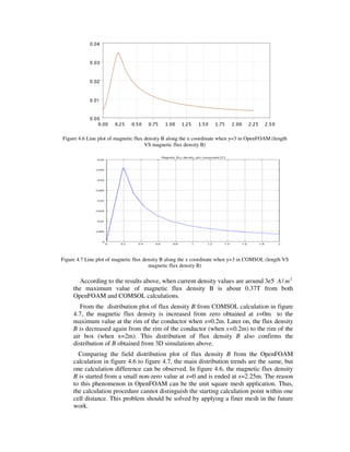
37. One problem should be pointed out that, in 2D axis-symmetric geometry, the A-V
solver can solve the electromagnetic problems with low electrical conductivity σ
values but not the cases with high electrical conductivity. The reason of this problem
has not been defined. But since the A-J solver will not involve any electrical
conductivityσ , it doesn’t have this issue at all.
4.2 Simulation Results of the Single Bar with Copper Ring
Relative permeability refers to a material’s ability to attract and conduct magnetic
lines of flux. The more conductive a material is to magnetic fields, the higher its
permeability [9]. As it is shown in the comparison figure 4.8, after setting a high
permeability (low reluctivity) in the steel bar in the middle of the ring-shape
conductor, the magnetic flux density B is confined to a path which closely couples
the ring –shape conductor and more flux density lines go through the more
conductive path- the steel bar. The simulation with the same geometry, boundary
conditions and initial values is done in COMSOL as well. The results are compared
in the left hand side pictures of fig 4.9 and 4.10.
Figure 4.8 Line plots comparison between cases with and without high permeability steel bar
4.3 Simulation Results of the Single Bar with a Copper Ring
and Permanent Magnets
As it is discussed in chapter 3.4.2, the initial values and boundary conditions in
table 3.11 are applied both in OpenFOAM and COMSOL. A coercive magnetic field
Hc with a value of (72400, 0, 0) is applied to represent permanent magnetic material
in both soft-wares. As it is shown in figure 4.9 and 4.10 (the two pictures at the right
side), coercive magnetic field Hc is applied along the x axis. The magnetic fields
distribution plots for geometries with (the plots at the right side) and without (the
plots at the left side) permanent magnetic materials are obtained from COMSOL and
OpenFOAM separately. Results are shown in figure 4.9 and figure 4.10.
Line Plot of
Magnetic Flux Density B
when Relative
Reluctivity=1 in steel bar
Line Plot of
Magnetic Flux Density B
when Relative
Reluctivity=5e-4 in steel bar

38. Figure 4.9 Surface plots from COMSOL
Figure 4.10 Surface plots from OpenFOAM
In both surface plots from COMSOL in figure 4.9 and OpenFOAM in figure 4.10,
the comparisons between the figures at the left side and the figures at the right side
show that, the magnetic flux density B is greatly increased after adding permanent
magnetic material.
Furthermore, the comparison between the two plots on the right side in figure 4.9
and figure 4.10 shows better computing ability in OpenFOAM than COMSOL for
this 3D simulation case including a permanent magnet. In OpenFOAM, a suitable
mesh approach can be decided according to the complexity of one specific
geometry. For this simulation done by the author, COMSOL can only solve this
problem with ‘coarser’ mesh because of the limitation of computer memory, which
gives the worse field distribution stream line as plot of 4.9 (to the right).
x
z
y
x
y
z

39. On the other hand, regarding to this simulation in OpenFOAM, there is no inner
boundary that can be set for the permanent magnetic block. Meanwhile, the size of
the permanent magnet block is defined by setting application areas of coercive
magnetic field in funkySetField utility as it is shown in chapter 3. Hereby, the
minimum length of each mesh volume on every dimension for a 3D geometry will
influence the accuracy of the calculation. For example, the thickness in the z
direction of the permanent magnet block is 0.2m in this simulation. If 40 cells are
chosen for a 6 m long geometry, the maximum cell length will be 0.15m along z,
which can bring large errors into the calculation. In this simulation, 60 cells are
applied for the magnet block on the z direction to avoid this mistake.
4.4 Simulation Results Comparison of Force Calculation
Force calculations are applied for two parallel current carrying bars. In order to
obtain the infinite long and thin bars, 10m as length and 0.4m as width are applied
for both bars. The distance between two bars from centre to centre is 0.6m.
4.4.1 Field Distribution Comparison between OpenFOAM and COMSOL
In figure 4.11, the surface plots of force density distribution calculated from
OpenFOAM and COMSOL are compared. For the convenience of the following
discussion, the terms ‘inner edge’ and ‘outer edge’ are defined as shown in figure
4.11. Both plots illustrate that the forces acting on the inner edges of two parallel
cables are larger than the forces acting on the outer edges. Further the shorter
distance between the two bars, the larger the magnetic force is.
Figure 4.11 Surface plots of force density distribution from OpenFOAM and COMSOL calculations
surface plot of Lorenz Force density
in OpenFOAM
surface plot of Lorenz Force density
in COMSOL
inner
edge
outer
edge left right
x dimension

40. 4.4.2 Numerical Results of Lorenz Force Method and Maxwell Stress Tensor
Method
Both the Lorenz force method and the Maxwell stress tensor method are applied
in OpenFOAM. The numerical values of the magnetic force from the OpenFOAM
calculation are given in table 4.5.
Table 4.5 Numerical values comparison of magnetic forces calculated by two different methods in
OpenFOAM
Results by Lorenz Force method in OpenFOAM (N/m)
Force acting on the left cable (-1.57206e-07 -7.64703e-23 0)
Force acting on the right cable (1.57206e-07 -7.41412e-23 0)
Results by the Maxwell Stress Tensor method in OpenFOAM (N/m)
Force on the Left Cable
Force on surface 1 (1.20408e-08 -1.2851e-23 0)
Force on surface 2 (-1.61322e-07 5.35406e-23 0)
Force on surface 3 (-3.98597e-09 -3.3557e-09 0)
Force on surface 4 (-3.98597e-09 3.3557e-09 0)
Force acting on left cable (-1.57253e-07 6.4851e-23 0)
Force on the Right Cable
Force on surface 1 (1.61322e-07 -3.90662e-23 0)
Force on surface 2 (-1.20408e-08 -1.44123e-23 0)
Force on surface 3 (3.98597e-09 -3.3557e-09 0)
Force on surface 4 (3.98597e-09 3.3557e-09 0)
Force acting on the right cable (1.57253e-07 -7.94093e-23 0)
In order to simplify the calculation in COMSOL, a 2D simulation instead of a 3D
simulation is taken. The same initial values are applied in COMSOL as the ones applied
in OpenFOAM. The magnetic forces calculated by the Lorenz Force method in
COMSOL are obtained in table 4.6. Figure 4.12 uses a bar chart to show the differences
between the OpenFOAM calculation and the COMSOL calculation.
Table 4.6 Results by the Lorenz force calculation in COMSOL
Results by the Lorenz Force method in COMSOL (N/m)
Force acting on the left cable -1.55704e-07
Force acting on the right cable 1.557316e-07

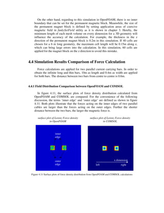
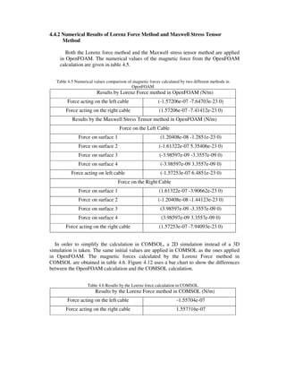
41. Figure 4.12 Results comparison on force calculation
As the results shows in figure 4.12, with opposite current direction flowing in the two
cables, the left side cable undertakes a force pointing to the left direction and vice versa.
In other words, a repulsive force is applied to both of the cables. And when 1A of current
is flowing though two parallel cuboid cables, the force between them is around 1.57e-
7N/m according to the OpenFOAM calculation. Compared to the COMSOL case with the
same geometry and boundary condition and initial values, the repulsive force is around
1.55e-7N/m. Figure 4.12 shows that the force calculation difference which acts on the
right or left cable is less than 0.1%, which shows great calculation accuracy in
OpenFOAM.
Since the force calculation is based on the first calculation results of electromagnetic
fields, new errors will be introduced which can be quite large. For the Maxwell Stress
Tensor method, the solution also depends on the choice of the integration path which will
bring calculation results difference for different paths [10].
Force(N/m)

42. 5 Conclusions and Future Work
By utilizing the huge calculation potential of OpenFOAM, this thesis work focuses on
solving static electromagnetic fields problems and force calculation problems. Hence, the
task of extending the calculation solvers library OpenFOAM software is successfully
accomplished. The finished tests and calculations by this thesis work are shown in table
5.1.
Table 5.1 Thesis coverage list
No. solver Case function
1 A-V solver SingleBarCase3D1 Electromagnetic fields of a single bar
conductor in 3D geometry
2 A-J solver SingleBarCase3D2 Electromagnetic fields of a single bar
conductor in 3D geometry
3 A-V solver SingleBarCase2D1 Electromagnetic fields of a single bar
conductor in 2D axis-symmetric
geometry
4 A-J solver SingleBarCase2D2 Electromagnetic fields of a single bar
conductor in 2D axis-symmetric
geometry
4 A-J solver with Hc tubeandbarCase16 Electromagnetic fields of a single bar and
a copper ring in 3D
5 A-J solver with Hc tbmCase12 Electromagnetic fields of a single bar and
a copper ring and a permanent magnet
block in 3D
6 A-J solver with
force calculation
2barsCase17 Force calculation for two parallel cable
After comparisons between COMSOL simulations and OpenFOAM simulations,
OpenFOAM shows its calculation possibilities and accuracy on electromagnetic field
problems and its calculation potential especially for finer mesh geometries.
In a long run, these basic calculations can be applied into the analysis of complex
electromagnetic devices such as electrical machines in, for instance electric vehicles, to
achieve less loss and an optimal design. Besides, this report also illustrates OpenFOAM
solver compilation and case application procedures clearly, which can be examples for
the new learner of OpenFOAM.
Because of the time limitation of this thesis work, there are still a lot of interesting
tasks left to be studied next.
Transient solvers and non-linear material application in OpenFOAM can be two
important study directions. Furthermore, though the editable solver is one of the
advantages of OpenFOAM, a manual geometry generated method is not so practical for
complex machine simulations. So, the mesh transfer utilization in OpenFOAM should be
paid attention to and applied for the next investigation step. Based on these works, a
movable mesh generation approach should be figured out to simulate movements of real
machines.

43. In general, a more complex mesh takes more simulation time. From the perspective of
simulation speed, OpenFOAM has its great advantage to handle parallel computing,
which can divide one task into several processors in order to decrease the total simulation
time. Along with more and more complex mesh, parallel computing utility should be
another research division of OpenFOAM.

44. Appendix 1
Mesh generation in file constant/polyMesh/blockMeshDict by ‘blockMesh’ utility of
‘SingleBarCase3D1’
/*---------------------------------------------------------------------------*
| ========= | |
| / F ield | OpenFOAM: The Open Source CFD Toolbox |
| / O peration | Version: 1.5 |
| / A nd | Web: http://www.openfoam.org |
| / M anipulation | |
*---------------------------------------------------------------------------*/
FoamFile
{
version 2.0;
format ascii;
class dictionary;
object blockMeshDict;
}
// * * * * * * * * * * * * * * * * * * * * * * * * * * * * * * * * * * * * * //
convertToMeters 1;
vertices
(
(-0.2 0.2 0) //0
(0.2 0.2 0) //1
(0.2 -0.2 0) //2
(-0.2 -0.2 0) //3
(-2 2 0) //4
(2 2 0) //5
(2 -2 0) //6
(-2 -2 0) //7
(-2 -0.2 0) //8
(-2 0.2 0) //9
(2 0.2 0) //10
(2 -0.2 0) //11
(-0.2 2 0) //12
(0.2 2 0) //13

45. (0.2 -2 0) //14
(-0.2 -2 0) //15
(-0.2 0.2 6) //16
(0.2 0.2 6) //17
(0.2 -0.2 6) //18
(-0.2 -0.2 6) //19
(-2 2 6) //20
(2 2 6) //21
(2 -2 6) //22
(-2 -2 6) //23
(-2 -0.2 6) //24
(-2 0.2 6) //25
(2 0.2 6) //26
(2 -0.2 6) //27
(-0.2 2 6) //28
(0.2 2 6) //29
(0.2 -2 6) //30
(-0.2 -2 6) //31
);
blocks
(
hex (0 3 2 1 16 19 18 17) (20 20 10) simpleGrading (1 1 1) //0
hex (1 2 11 10 17 18 27 26) (20 10 10) simpleGrading (1 1 1) //1
hex (2 14 6 11 18 30 22 27) (10 10 10) simpleGrading (1 1 1) //2
hex (3 15 14 2 19 31 30 18) (10 20 10) simpleGrading (1 1 1) //3
hex (8 7 15 3 24 23 31 19) (10 10 10) simpleGrading (1 1 1) //4
hex (9 8 3 0 25 24 19 16) (20 10 10) simpleGrading (1 1 1) //5
hex (4 9 0 12 20 25 16 28) (10 10 10) simpleGrading (1 1 1) //6
hex (12 0 1 13 28 16 17 29) (10 20 10) simpleGrading (1 1 1) //7
hex (13 1 10 5 29 17 26 21) (10 10 10) simpleGrading (1 1 1) //8
);
edges
(
);
patches
(
patch airleft //patch 0
(
(8 7 23 24) //face 0

46. (9 8 24 25) //face 1
(4 9 25 20) //2
)
patch airright // patch 1
(
(21 26 10 5) //3
(26 27 11 10) //4
(27 22 6 11) //5
)
patch airdown //patch 2
(
(4 20 28 12) //6
(12 28 29 13) //7
(13 29 21 5) //8
)
patch airup //patch 3
(
(14 6 22 30) //9
(15 14 30 31) //10
(7 15 31 23) //11
)
patch rod //patch 4
(
(0 1 2 3) //12
(16 19 18 17) //13
)
patch backandfront //patch 5
(
(1 10 11 2) //0
(2 11 6 14) //1
(3 2 14 15) //2
(8 3 15 7) //3
(9 0 3 8) //4
(4 12 0 9) //5
(12 13 1 0) //6
(13 5 10 1) //7
(18 27 26 17) //8
(30 22 27 18) //9

47. (31 30 18 19) //10
(23 31 19 24) //11
(24 19 16 25) //12
(25 16 28 20) //13
(16 17 29 28) //14
(17 26 21 29) //15
)
);
mergePatchPairs
(
);
// ************************************************************** //

48. Appendix 2
Boundary type definition in ‘constant /polyMesh /boundary’ file of
‘SingleBarCase3D2’
/*--------------------------------*- C++ -*----------------------------------*
| ========= | |
| / F ield | OpenFOAM: The Open Source CFD Toolbox |
| / O peration | Version: 1.6 |
| / A nd | Web: www.OpenFOAM.org |
| / M anipulation | |
*---------------------------------------------------------------------------*/
FoamFile
{
version 2.0;
format ascii;
class polyBoundaryMesh;
location "constant/polyMesh";
object boundary;
}
// * * * * * * * * * * * * * * * * * * * * * * * * * * * * * * * * * * * * * //
6
(
airleft
{
type patch;
nFaces 400;
startFace 45600;
}
airright
{
type patch;
nFaces 400;
startFace 46000;
}
airdown
{
type patch;
nFaces 400;
startFace 46400;

49. }
airup
{
type patch;
nFaces 400;
startFace 46800;
}
rod
{
type patch;
nFaces 800;
startFace 47200;
}
backandfront
{
type patch;
nFaces 2400;
startFace 48000;
}
)
// ********************************************************************* //

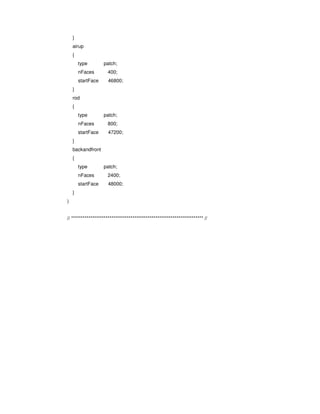
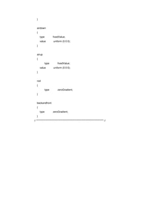
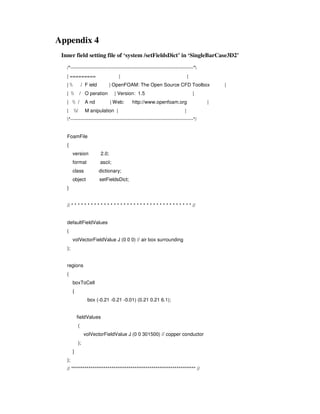
50. Appendix 3
Initial field setting file of ‘0 /A’ in ‘SingleBarCase3D1’
/*---------------------------------------------------------------------------*
| ========= | |
| / F ield | OpenFOAM: The Open Source CFD Toolbox |
| / O peration | Version: 1.4 |
| / A nd | Web: http://www.openfoam.org |
| / M anipulation | |
*---------------------------------------------------------------------------*/
// Field Dictionary
FoamFile
{
version 2.0;
format ascii;
class volVectorField;
object A;
}
// * * * * * * * * * * * * * * * * * * * * * * * * * * * * * * * * * * * * * //
dimensions [1 1 -2 0 0 -1 0];
internalField uniform (0 0 0);
boundaryField
{
airleft
{
type fixedValue;
value uniform (0 0 0);
}
airright
{
type fixedValue;
value uniform (0 0 0);

51. }
airdown
{
type fixedValue;
value uniform (0 0 0);
}
airup
{
type fixedValue;
value uniform (0 0 0);
}
rod
{
type zeroGradient;
}
backandfront
{
type zeroGradient;
}
// ********************************************************************* //

52. Appendix 4
Inner field setting file of ‘system /setFieldsDict’ in ‘SingleBarCase3D2’
/*---------------------------------------------------------------------------*
| ========= | |
| / F ield | OpenFOAM: The Open Source CFD Toolbox |
| / O peration | Version: 1.5 |
| / A nd | Web: http://www.openfoam.org |
| / M anipulation | |
*---------------------------------------------------------------------------*/
FoamFile
{
version 2.0;
format ascii;
class dictionary;
object setFieldsDict;
}
// * * * * * * * * * * * * * * * * * * * * * * * * * * * * * * * * * * * * * //
defaultFieldValues
(
volVectorFieldValue J (0 0 0) // air box surrounding
);
regions
(
boxToCell
{
box (-0.21 -0.21 -0.01) (0.21 0.21 6.1);
fieldValues
(
volVectorFieldValue J (0 0 301500) // copper conductor
);
}
);
// ***************************************************************** //

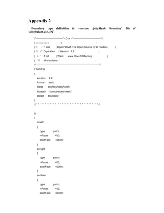
53. Appendix 5
.C file of A-J solver
#include "fvCFD.H"
// * * * * * * * * * * * * * * * * * * * * * * * * * * * * * * * * * * * * * //
int main(int argc, char *argv[])
{
# include "setRootCase.H"
# include "createTime.H"
# include "createMesh.H"
# include "createFields.H"
// * * * * * * * * * * * * * * * * * * * * * * * * * * * * * * * * * * * * * //
solve ( fvm::laplacian(A)==-muMag*J);
B= fvc::curl(A);
# include "IeEqn.H"
runTime++;
J.write();
A.write();
B.write();
Info<< "ExecutionTime = " << runTime.elapsedCpuTime() << " s"
<< " ClockTime = " << runTime.elapsedClockTime() << " s"
<< nl << endl;
return(0);
}
// ********************************************************************* //

54. References
1 http://openfoamwiki.net/index.php/Main_Page, “Main Page of Unofficial OpenFOAM
wiki”.
2 Christoph Schlensok, Thomas Scheermesser, Dirk van Riesen, and Gerhard
Henneberger, “Finite-Element Models of Electrical Machines and their Calculation”,
Institut fur Elektrische Maschinen, RWTH Aachen, Germany, 2003.
3 João Pedro A. Bastos Nelson Sadowski, “Electromagnetic Modeling by Finite
Element Methods”, Marcel Dekker, Inc, 2003, p. 35-285.
4 Marguerite Touma and Sonja Tidblad Lundmark, “Three-Dimensional Computation
of Eddy Currents in End Regions of Synchronous Generators”. Technical Report No.
231 L, Göteborg, Sweden 1996, p. 18-58.
5 Group CEDRAT, “Flux 10 user guide”. K101-10-EN-07/09, 2009, volume 3, p. 26-
104 and volume 4, p. 105.
6 Anogh V. Kank and S. V. Kulkarni, “Analysis of Lorenz and Saliency Forces in
Rotation Machines”, Indian Institute of Technology Bombay, Mumbai-400076.
7 Sonja Lundmark, “Review of force and torque calculations from numerical field
solutions”.
8 http://www.openfoam.com/, “Official Website of OpenFOAM”.
9 http://www.microwaves101.com/encyclopedia/highpermeability.cfm,“High
Permeability Materials”.
10 Stanley Humphries, “Theory and Application of the Maxwell Stress Tensor”.
Copyright 2010, p. 4.