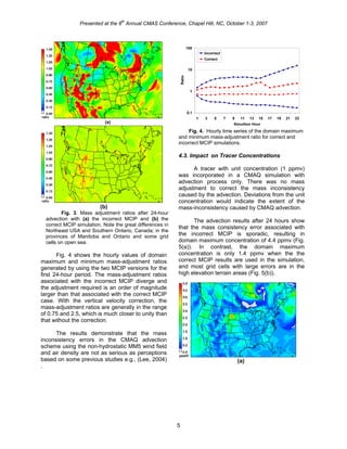
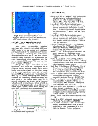
Presented at the 6
th
Annual CMAS Conference, Chapel Hill, NC, October 1-3, 2007
A CORRECTION TO MCIP CALCULATION OF VERTICAL CONTRAVARIANT
VELOCITY OF NON-HYDROSTATIC MM5 IN MCIP AND ITS IMPACT ON AIR
QUALITY SIMULATION
Fuquan Yang*, Jack Chen, Weimin Jiang, Helmut Roth, Steven C. Smyth,
Institute for Chemical Process and Environment Technology, National Research Council of Canada,
Ottawa, Ontario, Canada
1. INTRODUCTION
The contravariant vertical velocity used in the
Community Multi-scale Air Quality (CMAQ) Model
is calculated by the Meteorology-Chemistry
Interface Processor (MCIP). It is a key parameter
in controlling vertical advection and describing the
static stability of atmosphere. Large errors in the
vertical wind can significantly deteriorate the
consistency between the air density and wind
fields. Such consistency is a fundamental
requirement to ensure mass consistency in air
quality modeling studies (Byun, 1999).
Recently, we found an error in MCIP (version
3.2 and its earlier versions) in the computation of
the contravariant vertical wind velocity. Instead of
using the surface reference state pressure, the
total surface pressure from the first time period
processed by MCIP was mistakenly used in the
calculation of contravariant vertical velocity.
The error led to unphysical contravariant
vertical wind fields, caused exaggerated
perception of air mass inconsistency within the
non-hydrostatic MM5 meteorological model
outputs, and affected the advection scheme
analysis. After the error was reported, it was
subsequently corrected in the current release of
MCIP version 3.3.
This paper presents a detailed analysis of the
error and the correction. It also shows the impacts
of the correction on the extent of CMAQ mass
consistency adjustment and advected tracer
concentration.
2. CORRECTION OF THE
CONTRAVARIANT VERTICAL VELOCITY
ERROR
*Corresponding author: Fuquan Yang, National
Research Council of Canada, Room 233, M2,1200
Montreal Road, Ottawa, Ontario, Canada K1A 0R6; e-
mail: Fuquan.Yang@nrc-cnrc.gc.ca
2.1 Calculation of the contravariant vertical
velocity in MCIP
In MCIP, the contravariant vertical wind
velocity should be calculated as (Byun, 1999):
( ) ( ) w
p
g
mv
x
p
p
mu
x
p
p
pp
*
0
2
*
0
*
0
1
*
0
*
0
ˆˆ
ρσσ
ξ +
⎥
⎥
⎦
⎤
⎢
⎢
⎣
⎡
∂
∂
+
⎥
⎥
⎦
⎤
⎢
⎢
⎣
⎡
∂
∂
=& (1)
where, is the contravariant vertical wind
velocity, and are map scaled wind
velocities along the and direction, is
the normal vertical wind velocity component from
non-hydrostatic MM5,
ξ&
mu mv
1
ˆx 2
ˆx w
0pσ is the sigma value, 0ρ
is the reference state air density, g is
gravitational acceleration constant, and is the
difference between the reference state surface
pressure ( ) and the model top pressure ( ) ,
i.e.,
*
p
0sp tp
ts ppp −= 0
*
(2)
The reference state surface pressure can be
calculated from:
⎟
⎟
⎠
⎞
⎜
⎜
⎝
⎛
⎟
⎠
⎞
⎜
⎝
⎛
−−⎟
⎠
⎞
⎜
⎝
⎛
=
A
T
RA
gH
A
T
pps
00
2
00
000
2
exp
(3)
where R is the gas constant for dry air , H is the
terrain height, is the sea level pressure
(100,000Pa), is the temperature at (290
K), and
00P
00T 00P
A is the temperature lapse rate (50K),
representing the temperature difference between
and = 36788 Pa. The model reference
state does not change with time in the simulation.
00P eP /00
2.2 Error in the calculation of the contravariant
vertical velocity in previous MCIP versions
In the previous MCIP versions (version 3.2
and earlier), the in equation (1) was incorrectly
calculated as the difference between the total
*
p
1
Presented at the 6
th
Annual CMAS Conference, Chapel Hill, NC, October 1-3, 2007
surface pressure from the first time period
processed by MCIP ( ) and the pressure at the
model top, i.e.,
sp
tsincorrect ppp −=*
. (4)
The total surface pressure, , in Eq. (4) is
calculated by adding the perturbation pressure
sp
p′
from the first time period processed by MCIP to
the surface reference state pressure, i.e.,
ppp ss
′+= 0 (5)
where . From Eqs. (4) and (5), we can get:0spp <<′
tsincorrect pppp −′+= 0
*
. (6)
From Eqs.(2) and (6), it can be easily seen
that the perturbation pressure from the first time
period processed by MCIP was introduced into the
calculation of the incorrect in Eq. (4). The
incorrect was then used to calculate the
contravaraint vertical velocity in Eq. (1).
*
p
*
p
Note that this error exists only when the non-
hydrostatic MM5 results are processed by MCIP
and the vertical contravariant wind velocity
generated by MCIP is used in CMAQ. It does not
exist for the calculation of contravariant vertical
velocity with hydrostatic MM5 and has no impact
on CMAQ simulations that use the Yamartino
scheme where the contravariant vertical velocity is
recalculated in CMAQ.
2.3 Mathematical differences between the
incorrect and the correct contravariant vertical
velocities
Mathematically, the difference between the
incorrect and the correct contravariant vertical
wind velocities can be expressed as:
( )mu
x
p
px
p
p
pincorrect
incorrect
p
incorrect ⎥
⎦
⎤
⎢
⎣
⎡
∂
∂
−
∂
∂
=− 1
*
*
0
1
*
*
0
ˆˆ
σσ
ξξ &&
( )mv
x
p
px
p
p
pincorrect
incorrect
p
⎥
⎦
⎤
⎢
⎣
⎡
∂
∂
−
∂
∂
+ 2
*
*
0
2
*
*
0
ˆ
)
σσ
w
p
g
p
g
incorrect
⎟⎟
⎠
⎞
⎜⎜
⎝
⎛
−+ *
0
*
0 ρρ (7)
where and are the contravariant vertical
velocities calculated by the previous (v3.2 and
older) and the current (v3.3) MCIP versions,
respectively.
incorrectξ& ξ&
The three terms on the right-hand side can be
approximated as:
( ) )(
ˆˆˆ 1
'
*
0
1
*
*
0
1
*
*
0
mu
x
p
p
mu
x
p
px
p
p
ppincorrect
incorrect
p
∂
∂
≅⎥
⎦
⎤
⎢
⎣
⎡
∂
∂
−
∂
∂ σσσ (8)
( ) )(
ˆˆˆ 2
'
*
0
2
*
*
0
2
*
*
0
mv
x
p
p
mv
x
p
px
p
p
ppincorrect
incorrect
p
∂
∂
≅⎥
⎦
⎤
⎢
⎣
⎡
∂
∂
−
∂
∂ σσσ (9)
0*
0
*
0
≅⎟⎟
⎠
⎞
⎜⎜
⎝
⎛
− w
p
g
p
g
incorrect
ρρ (10)
The derivation processes for the above equations
are not given here for brevity.
From Eqs. (8), (9) and (10), it can be seen that
the difference of the contravariant vertical wind
velocity at a specified time is largely produced by
the contravariant horizontal wind velocity
( )mvmu, at that time and the gradient of
perturbation pressure (
1
'
ˆx
p
∂
∂ and 2
'
ˆx
p
∂
∂
) from the first
time period processed by MCIP.
The perturbation pressure from the first time
period processed by MCIP is kept to be constant
in the incorrect MCIP run and is used to calculate
the contravariant vertical velocity. Even for the
same non-hydrostatic MM5 output, the errors of
the contravariant vertical velocity generated by
different runs of the incorrect MCIP are different if
the runs start from different times.
Since the magnitude of formula Eq. (10)
approximates zero, the sign of the left hand side of
Eq. (7) is determined by the relative magnitudes of
the first two terms in the right hand side of the
equation, which can then be calculated
approximately by Eqs. (8) and (9).
There are two ideal situations in which the
sign of the left hand side of Eq. (7) can be
determined. First, when the signs of Eqs. (8) and
(9) are positive, a net positive upward
contravariant vertical wind is generated
( ). This can occur at grid cells which
are located southwest of a high perturbation
pressure center with southwest wind
(
0>−ξξ &&
incorrect
0,0
ˆ1
>>
∂
′∂
u
x
p ; 0,0
ˆ2
>>
∂
′∂
v
x
p ). Second, when the
2
Presented at the 6
th
Annual CMAS Conference, Chapel Hill, NC, October 1-3, 2007
signs of both Eqs. (8) and (9) are negative, a net
negative downward contravariant vertical wind is
produced ( ). This can occur at grid
cells which are located at the northeast of a low
perturbation pressure center with northeast wind
(
0<−ξξ &&
incorrect
0,0
ˆ1
<>
∂
′∂
u
x
p ; 0,0
ˆ2
<>
∂
′∂
v
x
p ).
When the signs of Eqs. (8) and (9) are
different, the sign of the left hand side of Eq. (7)
has to be determined by the relative magnitude of
Eqs. (8) and (9).
Since both the gradients of perturbation
pressure and horizontal winds are weak for high
perturbation pressure systems, the large
differences of vertical wind velocities are much
more pronounced in the low perturbation pressure
centers than that in the high perturbation pressure
centers
3. IMPACTS OF THE CORRECTION ON
THE CONTRAVARIANT VERTICAL
VELOCITIES GENERATED BY MCIP
3.1. Correlation of the vertical velocity error
with weather pattern
To investigate the contravariant vertical wind
velocity error and the impacts of the correction, the
non-hydrostatic MM5 was run for a 42-km grid
domain covering North America with 34 half-sigma
levels for July 15-20 2002. MM5 output was
processed with MCIPv3.2 (incorrect MCIP) and
MCIPv3.3 (correct MCIP). The Jacobian and air
density weighted contravariant vertical wind
velocity (WHAT_JD) from MCIPv3.2 is referred to
as the “incorrect vertical velocity” and that from
MCIPv3.3 is referred to as the “correct vertical
velocity”. Both MCIPv3.2 and MCIPv3.3 collapsed
the 34 layers in MM5 to 15 layers in MCIP.
As an example, Fig. 1(a) shows the surface
perturbation pressure at 00UTC July 16, which is
the beginning of the MCIP calculation, and the
horizontal wind vector at 06UTC, July 16, 2002,
and Fig. 1(b) shows the difference between the
incorrect and correct WHAT_JD (incorrect minus
correct values) at 06UTC, July 16. There are high
correlations between the locations of the low
perturbation pressure centers with strong western
winds and those grid cells where there are large
differences of vertical wind velocities. One deep
low perturbation pressure center with large vertical
wind difference can be seen over the northwestern
Atlantic Ocean. The scattered small scale low
perturbation pressure centers caused by high
elevation terrains in the southwest of the domain
also generate large differences of WHAT_JD.
(a)
(b)
Fig. 1(a). Surface perturbation pressure at 00UTC,
July, 16, and horizontal wind velocity vector at 06UTC,
July 16 (b). difference of Jacobian and air density
weighted contravariant vertical velocity (incorrect minus
correct values) at for 06UTC, July, 16.
3.2 Impact of the correction on the vertical
velocity when surface front passes
A weak surface front passes southern Ontario
around 18UTC (2pm EST), July 18 and terminates
a three-day ozone pollution episode. Fig. 2(a)
shows the hourly WHAT_JD values for the two
cases, and their difference (incorrect minus correct)
in the grid cell (99, 56), which is centered near
Hamilton in southern Ontario. Fig. 2(b) shows the
perturbation pressure at the first time step of the
MCIP run and surface horizontal wind fields at
18UTC (2pm EST), July 18, 2002 for the southern
Ontario areas. The upward vertical velocity is
weakest at 07UTC (3am EST), but regains its
peak value at 14UTC (10am EST). It weakens
3
Presented at the 6
th
Annual CMAS Conference, Chapel Hill, NC, October 1-3, 2007
again quickly after 18UTC (2pm EST) when the
front passes with intrusion of cold air (Fig. 2(a) ).
(a)
(b)
Fig. 2. (a) Hourly time series of the vertical wind
velocity for July 18, 2002 for grid (99,56), which is
centered with Hamilton, Southern Ontario; (b). Surface
horizontal wind vector at 2pm EST (18UTC), July 18,
2002 and perturbation pressure for 00UTC, 16, July,
2002 in the same grid cell
Before the fontal pass, there is a negative
difference in the vertical velocity because
0,0
ˆ1
><
∂
′∂
u
x
p , 0,0
ˆ2
≅≅
∂
′∂
v
x
p ( Fig. 2(b) ). The
correct MCIP gave larger vertical wind velocities
than the incorrect version. During the frontal
passage, the vertical velocity difference diminishes
because 0,0
ˆ1
≅<
∂
′∂
u
x
p and 0,0
ˆ2
<≅
∂
′∂
v
x
p . The
difference gradually shifts to positive after the front
passed because 0,0
ˆ1
<<
∂
′∂
u
x
p , 0,0
ˆ2
>≅
∂
′∂
v
x
p .
4. IMPACTS OF THE CORRECTION ON
CMAQ RESULTS
4.1. Impact on air density advection results
Air density is advected at each time step
and its ratio to the interpolated air density is used
to calibrate the mixing ratio of other species at
each step.
After 24 hours of advection, the incorrect
vertical wind velocity produces unphysical air
density with the domain maximum 6.9kg/m3
and
minimum 0.06kg/m3
. In contrast, the correct
vertical wind velocity produces more reasonable
air density, with the domain maximum 1.3 kg/m3
and minimum 0.44 kg/m3
(not shown).
4.2. Impact on Mass Consistency Adjustment
Hourly outputs from both the incorrect and
correct MCIP are used in CMAQ to quantify the
impact of the correction on mass consistency
adjustments required by the Parabolic Piecewise
Method (PPM) advection scheme used in CMAQ.
CMAQ employs two mass adjustment
approaches. The default “YAMO” approach
recalculates the vertical wind field with MCIP
horizontal contravariant wind components. The
MCIP error reported here does not affect the
advection results using this method.
The “DENRATE” approach in CMAQ
corrects concentration fields based on the ratio of
advected and interpolated air density, called
mass-adjustment ratio, at each advection time
step. The error in MCIP vertical contravariant
velocity significantly alters the mass consistency
adjustment ratio due to incorrect transport of the
air density ‘tracer’.
Fig. 3(a) and Fig. 3(b) show the spatial
distribution of the mass-adjustment ratio
calculated with the incorrect and correct MCIP,
respectively, after a 24 hour simulation. The air
density tracer is advected over 24 hours rather
than being updated at every advection time step.
Significant differences are observed both spatially
and in magnitude. Using the incorrect MCIP, the
adjustment ratio is more chaotic with magnitude
ranging from 0.17 to 22. In contrast, the correct
MCIP gives the ratio ranging from 0.76 to 2.5,
with few cells exceeding 1.5. The grid cells with
high ratios are mostly at the high elevation terrain
areas.
4
Presented at the 6
th
Annual CMAS Conference, Chapel Hill, NC, October 1-3, 2007
(a)
(b)
Fig. 3. Mass adjustment ratios after 24-hour
advection with (a) the incorrect MCIP and (b) the
correct MCIP simulation. Note the great differences in
Northeast USA and Southern Ontario, Canada; in the
provinces of Manitoba and Ontario and some grid
cells on open sea.
Fig. 4 shows the hourly values of domain
maximum and minimum mass-adjustment ratios
generated by using the two MCIP versions for the
first 24-hour period. The mass-adjustment ratios
associated with the incorrect MCIP diverge and
the adjustment required is an order of magnitude
larger than that associated with the correct MCIP
case. With the vertical velocity correction, the
mass-adjustment ratios are generally in the range
of 0.75 and 2.5, which is much closer to unity than
that without the correction.
The results demonstrate that the mass
inconsistency errors in the CMAQ advection
scheme using the non-hydrostatic MM5 wind field
and air density are not as serious as perceptions
based on some previous studies e.g., (Lee, 2004)
.
0.1
1
10
100
1 3 5 7 9 11 13 15 17 19 21 23
Simultion Hour
Ratio
Incorrect
Correct
Fig. 4. Hourly time series of the domain maximum
and minimum mass-adjustment ratio for correct and
incorrect MCIP simulations.
4.3. Impact on Tracer Concentrations
A tracer with unit concentration (1 ppmv)
was incorporated in a CMAQ simulation with
advection process only. There was no mass
adjustment to correct the mass inconsistency
caused by the advection. Deviations from the unit
concentration would indicate the extent of the
mass-inconsistency caused by CMAQ advection.
The advection results after 24 hours show
that the mass consistency error associated with
the incorrect MCIP is sporadic, resulting in
domain maximum concentration of 4.4 ppmv (Fig.
5(a)). In contrast, the domain maximum
concentration is only 1.4 ppmv when the the
correct MCIP results are used in the simulation,
and most grid cells with large errors are in the
high elevation terrain areas (Fig. 5(b)).
(a)
5
Presented at the 6
th
Annual CMAS Conference, Chapel Hill, NC, October 1-3, 2007
(b)
Fig. 5. Tracer concentrations after 24-hour
advection when (a) the incorrect and (b) the correct
MCIP results are used in the simulation.
5. CONCLUSION AND DISCUSSION
The mass inconsistency problem
associated with using non-hydrostatic MM5 and
MCIP results is not as serious as it has been
previously regarded. The problem is partly caused
by a mistake in calculating the contravariant
vertical wind velocity in MCIP. This error caused
incorrect tracer advection and exaggerated the
mass inconsistency ratios associated with the
non-hydrostatic MM5 results. The error has now
been corrected in MCIP3.3.
Although the sigma formulation in non-
hydrostatic MM5 allow the propagation of its
individual terrain features upward to all sigma
levels, even to the model top, this study shows
that the mass adjustment ratios at the middle
layers of CMAQ simulations are very close to unity
(see Fig. 6). When developing new advection
schemes, this consistency between air density and
wind fields in the middle layers need to be
carefully maintained and should not be disturbed
without sound physical basis. Efforts should be
spent to avoid propagating the errors at the lowest
sigma layers upward, which would destroy the
good mass consistency at the middle layers.
20
15
10
5
0
MassConsistencyAdjustmentRatio
1614121086420
Half Sigma Level
newMCIP
oldMCIP
Layer Maximum Value after 24 Hours
Fig. 6. Domain maximum mass adjustment ratios at
the model vertical half sigma layers
6. REFERENCES
Anthes, R.A. and T.T. Warner, 1978: Development
of hydrodynamic models suitable for air
pollution and other mesometeorological
studies. Mon. Wea. Rev., 106, 1045-1078.
Byun, D. W., 1999a: Dynamically consistent
formulations in meteorological and air quality
models for multiscale atmospheric studies.
Part I. Governing equations in a generalized
coordinate system. J. Atmos. Sci., 56, 3789-
3807.
Byun, D. W., 1999b: Dynamically consistent
formulations in meteorological and air quality,
models for multiscale atmospheric studies.
Part II: Mass conservations issues. J. Atmos
Sci., 56, 3808-3820.
Byun, D.W., and Ching, J.K.S., 1999: Science
algorithms of the EPA Models-3 Community
Multiscale Air Quality (CMAQ) Modeling
System, U.S. EPA/600/R-99/030.
Dudhia, J., 1993: A nonhydrostatic version of the
Penn State–NCAR, Mesoscale Model:
Validation tests. Mon. Wea. Rev., 121, 1493–
1513.
Dudhia J., Dave Gill, Kevin Manning, and Wei
Wang, 2005: PSU/NCAR Mesoscale Modeling
System Tutorial Class Notes and User’s Guide:
MM5 Modeling System, Version 3
Grell, G.A., J. Dudhia, and D.R. Stauffer, 1994: A
Description of the Fifth-Generation PENN
STATE/NCAR Mesoscale Model (MM5),
NCAR Technical Note, NCAR/TN-398+STR
Kitada, T., 1987: Effect of non-zero divergence
wind fields on atmospheric transport
calculations. Atmos. Environ., 21, 785–788
Klaus P. Hoinka and Günther Zängl., 2004: The
influence of the Vertical Coordinate on
Simulations of a PV Streamer Crossing the
Alps; Mon Wea Rev, 1860–1867
Lee, S.M., Yoon, S.C., and Byun D.W., 2004: The
effect of mass inconsistency of the
meteorological field generated by a common
meteorological model on air quality modeling.
Atmos. Environ. ,38, 2917-2926.
Murry L. Salby, 1996: Atmospheric physics, p166-
194
Pielke, R. A., 2002: Mesoscale Meteorological
Modeling. Academic Press, p122-160
Yin, D., 2004: A Description of the Extension for
Using Canadian GEM data in MCIP and a
Brief User’s Guide for GEM-MCIP. ICPET,
National Research Council of Canada.
6

Fuquan-Yang-MCIP-correrction-mass-inconsistency

  • 1.
    Presented at the6 th Annual CMAS Conference, Chapel Hill, NC, October 1-3, 2007 A CORRECTION TO MCIP CALCULATION OF VERTICAL CONTRAVARIANT VELOCITY OF NON-HYDROSTATIC MM5 IN MCIP AND ITS IMPACT ON AIR QUALITY SIMULATION Fuquan Yang*, Jack Chen, Weimin Jiang, Helmut Roth, Steven C. Smyth, Institute for Chemical Process and Environment Technology, National Research Council of Canada, Ottawa, Ontario, Canada 1. INTRODUCTION The contravariant vertical velocity used in the Community Multi-scale Air Quality (CMAQ) Model is calculated by the Meteorology-Chemistry Interface Processor (MCIP). It is a key parameter in controlling vertical advection and describing the static stability of atmosphere. Large errors in the vertical wind can significantly deteriorate the consistency between the air density and wind fields. Such consistency is a fundamental requirement to ensure mass consistency in air quality modeling studies (Byun, 1999). Recently, we found an error in MCIP (version 3.2 and its earlier versions) in the computation of the contravariant vertical wind velocity. Instead of using the surface reference state pressure, the total surface pressure from the first time period processed by MCIP was mistakenly used in the calculation of contravariant vertical velocity. The error led to unphysical contravariant vertical wind fields, caused exaggerated perception of air mass inconsistency within the non-hydrostatic MM5 meteorological model outputs, and affected the advection scheme analysis. After the error was reported, it was subsequently corrected in the current release of MCIP version 3.3. This paper presents a detailed analysis of the error and the correction. It also shows the impacts of the correction on the extent of CMAQ mass consistency adjustment and advected tracer concentration. 2. CORRECTION OF THE CONTRAVARIANT VERTICAL VELOCITY ERROR *Corresponding author: Fuquan Yang, National Research Council of Canada, Room 233, M2,1200 Montreal Road, Ottawa, Ontario, Canada K1A 0R6; e- mail: Fuquan.Yang@nrc-cnrc.gc.ca 2.1 Calculation of the contravariant vertical velocity in MCIP In MCIP, the contravariant vertical wind velocity should be calculated as (Byun, 1999): ( ) ( ) w p g mv x p p mu x p p pp * 0 2 * 0 * 0 1 * 0 * 0 ˆˆ ρσσ ξ + ⎥ ⎥ ⎦ ⎤ ⎢ ⎢ ⎣ ⎡ ∂ ∂ + ⎥ ⎥ ⎦ ⎤ ⎢ ⎢ ⎣ ⎡ ∂ ∂ =& (1) where, is the contravariant vertical wind velocity, and are map scaled wind velocities along the and direction, is the normal vertical wind velocity component from non-hydrostatic MM5, ξ& mu mv 1 ˆx 2 ˆx w 0pσ is the sigma value, 0ρ is the reference state air density, g is gravitational acceleration constant, and is the difference between the reference state surface pressure ( ) and the model top pressure ( ) , i.e., * p 0sp tp ts ppp −= 0 * (2) The reference state surface pressure can be calculated from: ⎟ ⎟ ⎠ ⎞ ⎜ ⎜ ⎝ ⎛ ⎟ ⎠ ⎞ ⎜ ⎝ ⎛ −−⎟ ⎠ ⎞ ⎜ ⎝ ⎛ = A T RA gH A T pps 00 2 00 000 2 exp (3) where R is the gas constant for dry air , H is the terrain height, is the sea level pressure (100,000Pa), is the temperature at (290 K), and 00P 00T 00P A is the temperature lapse rate (50K), representing the temperature difference between and = 36788 Pa. The model reference state does not change with time in the simulation. 00P eP /00 2.2 Error in the calculation of the contravariant vertical velocity in previous MCIP versions In the previous MCIP versions (version 3.2 and earlier), the in equation (1) was incorrectly calculated as the difference between the total * p 1
  • 2.
    Presented at the6 th Annual CMAS Conference, Chapel Hill, NC, October 1-3, 2007 surface pressure from the first time period processed by MCIP ( ) and the pressure at the model top, i.e., sp tsincorrect ppp −=* . (4) The total surface pressure, , in Eq. (4) is calculated by adding the perturbation pressure sp p′ from the first time period processed by MCIP to the surface reference state pressure, i.e., ppp ss ′+= 0 (5) where . From Eqs. (4) and (5), we can get:0spp <<′ tsincorrect pppp −′+= 0 * . (6) From Eqs.(2) and (6), it can be easily seen that the perturbation pressure from the first time period processed by MCIP was introduced into the calculation of the incorrect in Eq. (4). The incorrect was then used to calculate the contravaraint vertical velocity in Eq. (1). * p * p Note that this error exists only when the non- hydrostatic MM5 results are processed by MCIP and the vertical contravariant wind velocity generated by MCIP is used in CMAQ. It does not exist for the calculation of contravariant vertical velocity with hydrostatic MM5 and has no impact on CMAQ simulations that use the Yamartino scheme where the contravariant vertical velocity is recalculated in CMAQ. 2.3 Mathematical differences between the incorrect and the correct contravariant vertical velocities Mathematically, the difference between the incorrect and the correct contravariant vertical wind velocities can be expressed as: ( )mu x p px p p pincorrect incorrect p incorrect ⎥ ⎦ ⎤ ⎢ ⎣ ⎡ ∂ ∂ − ∂ ∂ =− 1 * * 0 1 * * 0 ˆˆ σσ ξξ && ( )mv x p px p p pincorrect incorrect p ⎥ ⎦ ⎤ ⎢ ⎣ ⎡ ∂ ∂ − ∂ ∂ + 2 * * 0 2 * * 0 ˆ ) σσ w p g p g incorrect ⎟⎟ ⎠ ⎞ ⎜⎜ ⎝ ⎛ −+ * 0 * 0 ρρ (7) where and are the contravariant vertical velocities calculated by the previous (v3.2 and older) and the current (v3.3) MCIP versions, respectively. incorrectξ& ξ& The three terms on the right-hand side can be approximated as: ( ) )( ˆˆˆ 1 ' * 0 1 * * 0 1 * * 0 mu x p p mu x p px p p ppincorrect incorrect p ∂ ∂ ≅⎥ ⎦ ⎤ ⎢ ⎣ ⎡ ∂ ∂ − ∂ ∂ σσσ (8) ( ) )( ˆˆˆ 2 ' * 0 2 * * 0 2 * * 0 mv x p p mv x p px p p ppincorrect incorrect p ∂ ∂ ≅⎥ ⎦ ⎤ ⎢ ⎣ ⎡ ∂ ∂ − ∂ ∂ σσσ (9) 0* 0 * 0 ≅⎟⎟ ⎠ ⎞ ⎜⎜ ⎝ ⎛ − w p g p g incorrect ρρ (10) The derivation processes for the above equations are not given here for brevity. From Eqs. (8), (9) and (10), it can be seen that the difference of the contravariant vertical wind velocity at a specified time is largely produced by the contravariant horizontal wind velocity ( )mvmu, at that time and the gradient of perturbation pressure ( 1 ' ˆx p ∂ ∂ and 2 ' ˆx p ∂ ∂ ) from the first time period processed by MCIP. The perturbation pressure from the first time period processed by MCIP is kept to be constant in the incorrect MCIP run and is used to calculate the contravariant vertical velocity. Even for the same non-hydrostatic MM5 output, the errors of the contravariant vertical velocity generated by different runs of the incorrect MCIP are different if the runs start from different times. Since the magnitude of formula Eq. (10) approximates zero, the sign of the left hand side of Eq. (7) is determined by the relative magnitudes of the first two terms in the right hand side of the equation, which can then be calculated approximately by Eqs. (8) and (9). There are two ideal situations in which the sign of the left hand side of Eq. (7) can be determined. First, when the signs of Eqs. (8) and (9) are positive, a net positive upward contravariant vertical wind is generated ( ). This can occur at grid cells which are located southwest of a high perturbation pressure center with southwest wind ( 0>−ξξ && incorrect 0,0 ˆ1 >> ∂ ′∂ u x p ; 0,0 ˆ2 >> ∂ ′∂ v x p ). Second, when the 2
  • 3.
    Presented at the6 th Annual CMAS Conference, Chapel Hill, NC, October 1-3, 2007 signs of both Eqs. (8) and (9) are negative, a net negative downward contravariant vertical wind is produced ( ). This can occur at grid cells which are located at the northeast of a low perturbation pressure center with northeast wind ( 0<−ξξ && incorrect 0,0 ˆ1 <> ∂ ′∂ u x p ; 0,0 ˆ2 <> ∂ ′∂ v x p ). When the signs of Eqs. (8) and (9) are different, the sign of the left hand side of Eq. (7) has to be determined by the relative magnitude of Eqs. (8) and (9). Since both the gradients of perturbation pressure and horizontal winds are weak for high perturbation pressure systems, the large differences of vertical wind velocities are much more pronounced in the low perturbation pressure centers than that in the high perturbation pressure centers 3. IMPACTS OF THE CORRECTION ON THE CONTRAVARIANT VERTICAL VELOCITIES GENERATED BY MCIP 3.1. Correlation of the vertical velocity error with weather pattern To investigate the contravariant vertical wind velocity error and the impacts of the correction, the non-hydrostatic MM5 was run for a 42-km grid domain covering North America with 34 half-sigma levels for July 15-20 2002. MM5 output was processed with MCIPv3.2 (incorrect MCIP) and MCIPv3.3 (correct MCIP). The Jacobian and air density weighted contravariant vertical wind velocity (WHAT_JD) from MCIPv3.2 is referred to as the “incorrect vertical velocity” and that from MCIPv3.3 is referred to as the “correct vertical velocity”. Both MCIPv3.2 and MCIPv3.3 collapsed the 34 layers in MM5 to 15 layers in MCIP. As an example, Fig. 1(a) shows the surface perturbation pressure at 00UTC July 16, which is the beginning of the MCIP calculation, and the horizontal wind vector at 06UTC, July 16, 2002, and Fig. 1(b) shows the difference between the incorrect and correct WHAT_JD (incorrect minus correct values) at 06UTC, July 16. There are high correlations between the locations of the low perturbation pressure centers with strong western winds and those grid cells where there are large differences of vertical wind velocities. One deep low perturbation pressure center with large vertical wind difference can be seen over the northwestern Atlantic Ocean. The scattered small scale low perturbation pressure centers caused by high elevation terrains in the southwest of the domain also generate large differences of WHAT_JD. (a) (b) Fig. 1(a). Surface perturbation pressure at 00UTC, July, 16, and horizontal wind velocity vector at 06UTC, July 16 (b). difference of Jacobian and air density weighted contravariant vertical velocity (incorrect minus correct values) at for 06UTC, July, 16. 3.2 Impact of the correction on the vertical velocity when surface front passes A weak surface front passes southern Ontario around 18UTC (2pm EST), July 18 and terminates a three-day ozone pollution episode. Fig. 2(a) shows the hourly WHAT_JD values for the two cases, and their difference (incorrect minus correct) in the grid cell (99, 56), which is centered near Hamilton in southern Ontario. Fig. 2(b) shows the perturbation pressure at the first time step of the MCIP run and surface horizontal wind fields at 18UTC (2pm EST), July 18, 2002 for the southern Ontario areas. The upward vertical velocity is weakest at 07UTC (3am EST), but regains its peak value at 14UTC (10am EST). It weakens 3
  • 4.
    Presented at the6 th Annual CMAS Conference, Chapel Hill, NC, October 1-3, 2007 again quickly after 18UTC (2pm EST) when the front passes with intrusion of cold air (Fig. 2(a) ). (a) (b) Fig. 2. (a) Hourly time series of the vertical wind velocity for July 18, 2002 for grid (99,56), which is centered with Hamilton, Southern Ontario; (b). Surface horizontal wind vector at 2pm EST (18UTC), July 18, 2002 and perturbation pressure for 00UTC, 16, July, 2002 in the same grid cell Before the fontal pass, there is a negative difference in the vertical velocity because 0,0 ˆ1 >< ∂ ′∂ u x p , 0,0 ˆ2 ≅≅ ∂ ′∂ v x p ( Fig. 2(b) ). The correct MCIP gave larger vertical wind velocities than the incorrect version. During the frontal passage, the vertical velocity difference diminishes because 0,0 ˆ1 ≅< ∂ ′∂ u x p and 0,0 ˆ2 <≅ ∂ ′∂ v x p . The difference gradually shifts to positive after the front passed because 0,0 ˆ1 << ∂ ′∂ u x p , 0,0 ˆ2 >≅ ∂ ′∂ v x p . 4. IMPACTS OF THE CORRECTION ON CMAQ RESULTS 4.1. Impact on air density advection results Air density is advected at each time step and its ratio to the interpolated air density is used to calibrate the mixing ratio of other species at each step. After 24 hours of advection, the incorrect vertical wind velocity produces unphysical air density with the domain maximum 6.9kg/m3 and minimum 0.06kg/m3 . In contrast, the correct vertical wind velocity produces more reasonable air density, with the domain maximum 1.3 kg/m3 and minimum 0.44 kg/m3 (not shown). 4.2. Impact on Mass Consistency Adjustment Hourly outputs from both the incorrect and correct MCIP are used in CMAQ to quantify the impact of the correction on mass consistency adjustments required by the Parabolic Piecewise Method (PPM) advection scheme used in CMAQ. CMAQ employs two mass adjustment approaches. The default “YAMO” approach recalculates the vertical wind field with MCIP horizontal contravariant wind components. The MCIP error reported here does not affect the advection results using this method. The “DENRATE” approach in CMAQ corrects concentration fields based on the ratio of advected and interpolated air density, called mass-adjustment ratio, at each advection time step. The error in MCIP vertical contravariant velocity significantly alters the mass consistency adjustment ratio due to incorrect transport of the air density ‘tracer’. Fig. 3(a) and Fig. 3(b) show the spatial distribution of the mass-adjustment ratio calculated with the incorrect and correct MCIP, respectively, after a 24 hour simulation. The air density tracer is advected over 24 hours rather than being updated at every advection time step. Significant differences are observed both spatially and in magnitude. Using the incorrect MCIP, the adjustment ratio is more chaotic with magnitude ranging from 0.17 to 22. In contrast, the correct MCIP gives the ratio ranging from 0.76 to 2.5, with few cells exceeding 1.5. The grid cells with high ratios are mostly at the high elevation terrain areas. 4
  • 5.
    Presented at the6 th Annual CMAS Conference, Chapel Hill, NC, October 1-3, 2007 (a) (b) Fig. 3. Mass adjustment ratios after 24-hour advection with (a) the incorrect MCIP and (b) the correct MCIP simulation. Note the great differences in Northeast USA and Southern Ontario, Canada; in the provinces of Manitoba and Ontario and some grid cells on open sea. Fig. 4 shows the hourly values of domain maximum and minimum mass-adjustment ratios generated by using the two MCIP versions for the first 24-hour period. The mass-adjustment ratios associated with the incorrect MCIP diverge and the adjustment required is an order of magnitude larger than that associated with the correct MCIP case. With the vertical velocity correction, the mass-adjustment ratios are generally in the range of 0.75 and 2.5, which is much closer to unity than that without the correction. The results demonstrate that the mass inconsistency errors in the CMAQ advection scheme using the non-hydrostatic MM5 wind field and air density are not as serious as perceptions based on some previous studies e.g., (Lee, 2004) . 0.1 1 10 100 1 3 5 7 9 11 13 15 17 19 21 23 Simultion Hour Ratio Incorrect Correct Fig. 4. Hourly time series of the domain maximum and minimum mass-adjustment ratio for correct and incorrect MCIP simulations. 4.3. Impact on Tracer Concentrations A tracer with unit concentration (1 ppmv) was incorporated in a CMAQ simulation with advection process only. There was no mass adjustment to correct the mass inconsistency caused by the advection. Deviations from the unit concentration would indicate the extent of the mass-inconsistency caused by CMAQ advection. The advection results after 24 hours show that the mass consistency error associated with the incorrect MCIP is sporadic, resulting in domain maximum concentration of 4.4 ppmv (Fig. 5(a)). In contrast, the domain maximum concentration is only 1.4 ppmv when the the correct MCIP results are used in the simulation, and most grid cells with large errors are in the high elevation terrain areas (Fig. 5(b)). (a) 5
  • 6.
    Presented at the6 th Annual CMAS Conference, Chapel Hill, NC, October 1-3, 2007 (b) Fig. 5. Tracer concentrations after 24-hour advection when (a) the incorrect and (b) the correct MCIP results are used in the simulation. 5. CONCLUSION AND DISCUSSION The mass inconsistency problem associated with using non-hydrostatic MM5 and MCIP results is not as serious as it has been previously regarded. The problem is partly caused by a mistake in calculating the contravariant vertical wind velocity in MCIP. This error caused incorrect tracer advection and exaggerated the mass inconsistency ratios associated with the non-hydrostatic MM5 results. The error has now been corrected in MCIP3.3. Although the sigma formulation in non- hydrostatic MM5 allow the propagation of its individual terrain features upward to all sigma levels, even to the model top, this study shows that the mass adjustment ratios at the middle layers of CMAQ simulations are very close to unity (see Fig. 6). When developing new advection schemes, this consistency between air density and wind fields in the middle layers need to be carefully maintained and should not be disturbed without sound physical basis. Efforts should be spent to avoid propagating the errors at the lowest sigma layers upward, which would destroy the good mass consistency at the middle layers. 20 15 10 5 0 MassConsistencyAdjustmentRatio 1614121086420 Half Sigma Level newMCIP oldMCIP Layer Maximum Value after 24 Hours Fig. 6. Domain maximum mass adjustment ratios at the model vertical half sigma layers 6. REFERENCES Anthes, R.A. and T.T. Warner, 1978: Development of hydrodynamic models suitable for air pollution and other mesometeorological studies. Mon. Wea. Rev., 106, 1045-1078. Byun, D. W., 1999a: Dynamically consistent formulations in meteorological and air quality models for multiscale atmospheric studies. Part I. Governing equations in a generalized coordinate system. J. Atmos. Sci., 56, 3789- 3807. Byun, D. W., 1999b: Dynamically consistent formulations in meteorological and air quality, models for multiscale atmospheric studies. Part II: Mass conservations issues. J. Atmos Sci., 56, 3808-3820. Byun, D.W., and Ching, J.K.S., 1999: Science algorithms of the EPA Models-3 Community Multiscale Air Quality (CMAQ) Modeling System, U.S. EPA/600/R-99/030. Dudhia, J., 1993: A nonhydrostatic version of the Penn State–NCAR, Mesoscale Model: Validation tests. Mon. Wea. Rev., 121, 1493– 1513. Dudhia J., Dave Gill, Kevin Manning, and Wei Wang, 2005: PSU/NCAR Mesoscale Modeling System Tutorial Class Notes and User’s Guide: MM5 Modeling System, Version 3 Grell, G.A., J. Dudhia, and D.R. Stauffer, 1994: A Description of the Fifth-Generation PENN STATE/NCAR Mesoscale Model (MM5), NCAR Technical Note, NCAR/TN-398+STR Kitada, T., 1987: Effect of non-zero divergence wind fields on atmospheric transport calculations. Atmos. Environ., 21, 785–788 Klaus P. Hoinka and Günther Zängl., 2004: The influence of the Vertical Coordinate on Simulations of a PV Streamer Crossing the Alps; Mon Wea Rev, 1860–1867 Lee, S.M., Yoon, S.C., and Byun D.W., 2004: The effect of mass inconsistency of the meteorological field generated by a common meteorological model on air quality modeling. Atmos. Environ. ,38, 2917-2926. Murry L. Salby, 1996: Atmospheric physics, p166- 194 Pielke, R. A., 2002: Mesoscale Meteorological Modeling. Academic Press, p122-160 Yin, D., 2004: A Description of the Extension for Using Canadian GEM data in MCIP and a Brief User’s Guide for GEM-MCIP. ICPET, National Research Council of Canada. 6