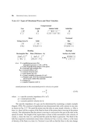
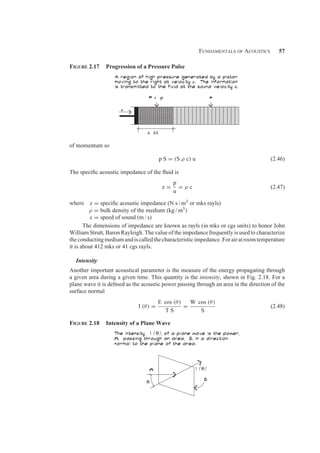
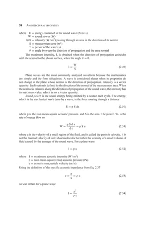
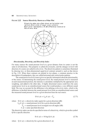
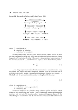
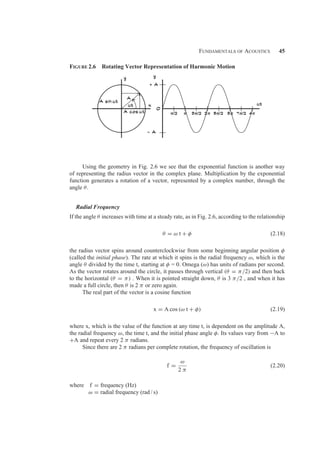
The document discusses the fundamentals of acoustics, focusing on concepts such as frequency and wavelength, harmonic motion, and the nature of sound waves. It explains the relationship between frequency, wavelength, and speed of sound, and introduces the concepts of simple harmonic motion, complex numbers, and wave superposition. Additionally, it covers the measurement of sound spectra and the use of filters in acoustic analysis.

![Fundamentals of Acoustics 51
element in the direction of propagation, which transfer energy through alternations of high
pressure and low velocity with low pressure and high velocity. It is the material properties
of mass and elasticity that ensure the propagation of the wave.
As a wave propagates through a medium such as air, the particles oscillate back and
forth when the wave passes. We can write an equation for the functional behavior of the
displacement y of a small volume of air away from its equilibrium position, caused by a
wave moving along the positive x axis (to the right) at some velocity c.
y = f(x − c t) (2.31)
Implicit in this equation is the notion that the displacement, or any other property of the
wave, will be the same for a given value of (x − c t). If the wave is sinusoidal then
y = A sin [k (x − c t)] (2.32)
where k is called the wave number and has units of radians per length. By comparison to
Eq. 2.19 the term (k c) is equal to the radial frequency omega.
k =
2 π
λ
=
ω
c
(2.33)
Wavelength of Sound
The wavelength of a sound wave is a particularly important measure. Much of the behavior
of a sound wave relates to the wavelength, so that it becomes the scale by which we judge
the physical size of objects. For example, sound will scatter (bounce) off a flat object that is
several wavelengths long in a specular (mirror-like) manner. If the object is much smaller
than a wavelength, the sound will simply flow around it as if it were not there. If we observe
the behavior of water waves we can clearly see this behavior. Ocean waves will pass by small
rocks in their path with little change, but will reflect off a long breakwater or similar barrier.
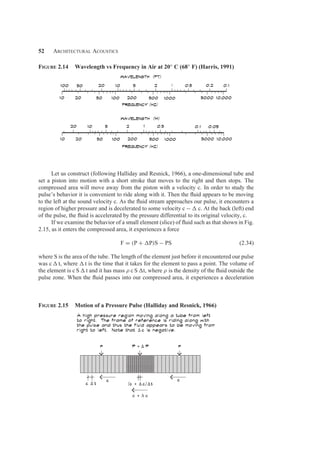
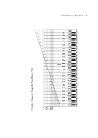
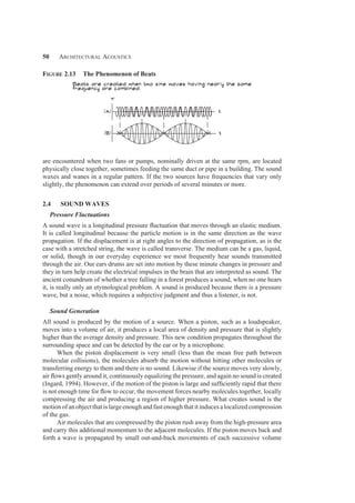
Figure2.14showstypicalvaluesofthewavelengthofsoundinairatvariousfrequencies.
At 1000 Hz, which is in the middle of the speech frequency range, the wavelength is about
0.3 m (1 ft) while for the lowest note on the piano the wavelength is about 13 m (42 ft). The
lowest note on a large pipe organ might be produced by a 10 m (32 ft) pipe that is half the
wavelength of the note. The highest frequency audible to humans is about 20,000 Hz and has
a wavelength of around half an inch. Bats, which use echolocation to find their prey, must
transmit frequencies as high as 100,000 Hz to scatter off a 2 mm (0.1 in) mosquito.
Velocity of Sound
The mathematical description of the changes in pressure and density induced by a sound
wave, which is called the wave equation, requires that certain assumptions be made about
the medium. In general we examine an element of volume (say a cube) small enough to
smoothly represent the local changes in pressure and density, but large enough to contain
very many molecules. When we mathematically describe physical phenomena created by a
sound wave, we are talking about the average properties associated with such a small volume
element.](https://image.slidesharecdn.com/acousticsnotes1-250212105117-d9d54111/85/fundamental-of-engineering-Acoustics_notes1-pdf-15-320.jpg)