Download as PDF, PPTX


![> hist(Val$AMEX, breaks=20, main="Distribution
AMEX Returns")
> sd(Val$AMEX)
[1] 0.01915489
ESGF 5IFM Q1 2012
vinzjeannin@hotmail.com
> hist(Val$SPX, breaks=20, main="Distribution
SPXX Returns")
> sd(Val$SPX)
[1] 0.01468776 26](https://image.slidesharecdn.com/financialeconometricmodelsi-13274911680315-phpapp02-120125053516-phpapp02/85/Financial-Econometric-Models-I-26-320.jpg)
![These are obvious negatively skewed distributions
ESGF 5IFM Q1 2012
Reminders
3
− − 3
= =
− 2 3/2
vinzjeannin@hotmail.com
• Negative skew: long left tail, mass on the right, skew to the left
• Positive skew: long right tail, mass on the left, skew to the right
> skewness(Val$AMEX)
[1] -0.2453693
> skewness(Val$SPX) 27
[1] -0.4178701](https://image.slidesharecdn.com/financialeconometricmodelsi-13274911680315-phpapp02-120125053516-phpapp02/85/Financial-Econometric-Models-I-27-320.jpg)
![These are obvious leptokurtic distributions
ESGF 5IFM Q1 2012
Reminders
4
− − 4
= =
− 2 2
vinzjeannin@hotmail.com
> library(moments)
> kurtosis(Val$AMEX) What is their K?
[1] 5.770583 (excess kurtosis)
> kurtosis(Val$SPX)
[1] 5.671254 28
Subtract 3 to make it relative to the
normal distribution…](https://image.slidesharecdn.com/financialeconometricmodelsi-13274911680315-phpapp02-120125053516-phpapp02/85/Financial-Econometric-Models-I-28-320.jpg)


![By the way, what is the most platykurtic distribution in the nature?
Toss it!
ESGF 4IFM Q1 2012
Head = Success = 1 / Tail = Failure = 0
vinzjeannin@hotmail.com
> require(moments)
> library(moments)
> toss<-rbinom(10000000,1,0.5)
> mean(toss)
[1] 0.5001777
> kurtosis(toss)
[1] 1.000001
> kurtosis(toss)-3
[1] -1.999999
> hist(toss, breaks=10,main="Tossing a
coin 10 millions times",xlab="Result
of the trial",ylab="Occurence") 31
> sum(toss)
[1] 5001777](https://image.slidesharecdn.com/financialeconometricmodelsi-13274911680315-phpapp02-120125053516-phpapp02/85/Financial-Econometric-Models-I-31-320.jpg)


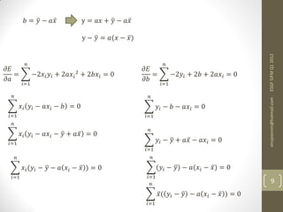
The document summarizes a session on financial econometric models. It will introduce models, their objectives of describing, modeling and forecasting data behavior. It will cover ordinary least squares regression, estimating intercepts and slopes to minimize residuals. It will also discuss calculating variances, covariances, correlation coefficients and assessing the quality of regressions. Examples using Excel functions like intercept, slope, var.p, covariance.p and stdev.p will be covered.