Financial Analysis Text

1
Financial Analysis of PepsiCo.
FNC 474-01
Intermediate Financial Management
Tyree Etheridge
October 20, 2015

2
Table of Contents
Introduction & History of PepsiCo.
Chapter 1: Financial Ratio Analysis of PepsiCo.
Chapter 2: The Extended DuPont System of Financial
Analysis
Chapter 3: The Long-term Growth Rate
Chapter4: TheBeta Coefficient & RequiredRateof Return
on Equity of PepsiCo.
Chapter 5: Free Cash Flow to Equity of PepsiCo.
Chapter 6: Valuing PepsiCo.

3
Introduction
PepsiCo, as it’s named today, was not always the company it is now. The soft drink giant
began its life as the 1893 creation of Caleb Davis Bradham, a North Carolina pharmacist who
created the drink to aid in digestion. The original mixture created by Bradham was made using
water, caramel, sugar, lemon oil, nutmeg, and other ingredients and was named Brad’s drink
after its creator. Brad’s drink was an immediate success among Bradham’s drugstore clients as it
was thought of as a healthy daily beverage. In August 1898, Caleb Bradham renamed his
beverage from Brad’s drink to Pepsi-Cola after purchasing the Pep Cola name from a competitor
for $100 and in 1902 formed the Pepsi-Cola company. The rising demand for the original Pepsi
syrup caused Bradham to trademark the mixture and name on June 16, 1903. Within its first
year of business, Pepsi-Cola sold 7,968 gallons and by 1904 Pepsi-Cola was selling
approximately 20,000 gallons of the syrup annually. The original Pepsi logo was designed by
Bradham’s artist of a neighbor in 1903. By 1904 Caleb Bradham had purchased a building in
New Bern, North Carolina to house Pepsi’s bottling operations and by 1906 there were 15
bottling plants resulting in syrup sales of 38,605 gallons. Pepsi was originally sold in 6 ounce
glass bottles with the Pepsi logo on the front until 1934 when Pepsi began offering 12 ounce
bottles for 5 cents.
Throughout the years from the early 1900’s to WWI, Pepsi grew exponentially and saw
great success; however, the firm suffered hard times during the years of WWI as the price of
sugar rose since it was being rationed by the U.S. government. The rationing and price of sugar
kept Pepsi from being able to meet its consumers’ supply demands. Despite Caleb Bradham’s
attempts at producing a sugar substitute, Pepsi fell short of major demand needs and ultimately
forced Caleb Bradham and Pepsi to file bankruptcy on May 31, 1923, with its assets being sold

4
for $30,000 to Craven Holding Corporation. In the same year Craven Holdings sold Pepsi to a
Wall Street broker named Roy C. Megargel, who purchased the firm for $35,000 forming the
Pepsi-Cola Corporation. After several years of continuous profit loss, Megargel was forced to
file bankruptcy; the second bankruptcy for Pepsi Cola. The firm was purchased in 1931 by
Charles G. Guth, president of the Loft Candy Company. In 1934 it was Guth who decided to
double the size of the Pepsi bottle to 12 ounces and sell it for 5 cents a bottle. In 1940 Pepsi
made history being the first company to have a nationally broadcast jingle with its “Nickel
Nickel” advertisement for the 5 cent 12 ounce bottle.
Pepsi continued to flourish for the next 30 years making major acquisitions along the way
such as its 1964 introduction of diet Pepsi as well as the acquisition of Mountain Dew from the
Tip Corporation. The following year Pepsi-Cola merged with Frito-Lay, a snack foods company
created in 1938 by Herman Lay. This merger created the Pepsi Corporation also known as Pepsi-
Co. After this successful merger, Pepsi-Co began a series of acquisitions of brands outside of its
soft drink industry such as Pizza Hut, Taco Bell, California Pizza Kitchen, and Wilson Sporting
Goods to name a few. PepsiCo held on to these acquisitions until 1997 when it sold some and
spun the others off into a new firm named Tricon Global Restaurants which was later renamed as
Yum Brands. In 2006 PepsiCo named Indra K Nooyi as its Chief Executive Officer, the first
female CEO in Pepsi’s 100 year history. Prior to becoming the CEO, Nooyi was the firm’s Chief
Financial Officer for five years. Prior to that she was Senior Vice President of Strategic Planning
for four years. As Chief Executive Officer, Indra Nooyi has directed Pepsi’s global strategy for
more than 8 years.

5
Chapter 1: Financial Ratio Analysis
Financial Statements
The financial statements for PepsiCo were retrieved from EDGAR SEC and included the
consolidated statement of income, consolidated balance sheets, and the consolidated statement of
cash flows. The ticker symbol for PepsiCo was retrieved from Yahoo Finance: EDGAR refers to
the Electronic Data Gathering Analysis and Retrieval system, operated by the Securities and
Exchange Commission. The statements of PepsiCo. Were pulled from the ten previous years of
10-K documents. The data retrieved from the consolidated statement of income includes sales,
cost of goods sold, operating expenses, EBIT, interest expense, and net income, while the
consolidated balance sheet gives us accounts receivable, inventory, current assets, depreciation,
net fixed assets, accounts payable, current liabilities, long-term debt, retained earnings, total
owners’ equity, total liabilities, and owners’ equity and shares outstanding. The data retrieved
from the consolidated statement of cash flows includes dividends, historical stock prices, and
historical shares outstanding for the last 11 years.

6
Financial Ratio Analysis
Financial ratio analysis is the quantitative analysis of information contained in a
company’s financial statements. It’s commonly utilized by investors to value firms for purchase.
Financial ratio analysis serves as an evaluation tool used to analyze a firm’s financial standing.
These ratios are commonly used to compare different firms within the same industry. Financial
ratios fall under five categories: liquidity ratios, asset management ratios, financial leverage
ratios, profitability ratios, and market based ratios.

8
Liquidity Ratios
Liquidity ratios measure the firm’s ability to pay off short term debts and obligations.
These ratios are metrics used to ensure that the firm has the required amount of cash and short
term assets that include accounts receivables and inventories, which are used to meet short term
debts such as accounts payable. It is generally understood that the higher the liquidity ratio, the
greater the ability that the firm has to meet short term obligations. There are two liquidity ratios,
which are the current ratio and the quick ratio. The current ratio is also known as the working
capital ratio and is the going concern that indicates the amount of short-term assets that firm has
with relation to each dollar of short-term liabilities and is calculated by dividing the firm’s
current assets by its current liabilities. The quick ratio is the ratio that is used to measure a firm’s
short term liquidity, or its abilities to meet short term obligations when inventory is not being
properly converted into cash. Ultimately the quick ratio measures the dollar amount of liquid
assets available for each dollar of current liabilities and is calculated by subtracting inventories
from current assets and dividing that number by current liabilities.

9
Asset Management Ratios
Assets are the most valuable aspects of any firm, and therefore, should be maintained and
ensured against error. Asset management ratios measures how efficiently the firm utilizes these
assets to generate business. There are four asset management ratios: day’s sales outstanding,
inventory turnover, net fixed assets, and total asset turnover. The day’s sales outstanding ratio
measures the average number of days it takes a company to collect revenue (accounts receivable)
once a sale has been made. While a small day’s sales outstanding value means that it’s taking a
firm a short amount of time to collect its revenue, a large day’s sales outstanding value means
that it’s taking a firm a long amount of time to collect its accounts receivable. The day’s sales
outstanding ratio can be calculated by dividing annual sales by 365, then dividing that number
into receivables. The inventory turnover ratio shows the amount of times that that the inventory
of a firm is sold and replaced over a fixed period. In addition the inventory turnover ratio also
depicts how many dollars of sales the company generates for each dollar of inventory and is

10
calculated by dividing sales by inventory. Net fixed assets turnover measures the number of
dollars of sales generated for each dollar of inventory and is calculated by dividing sales over
fixed assets. The highest level for net fixed asset turnover was .33 in 2006 and the lowest being
.26 in 2014. Total dollar of total assets. It is calculated by dividing sales over total assets asset
turnover ratio refers to the number of dollars of sales generated for each sale. The highest total
asset turnover ratio was 1.20 in 2008 while the lowest value was .75 in 2011.

11
Financial Leverage Ratios
Financial leverage ratios indicate how much debt and owner’s equity the firm uses to
finance its operations, or simply the extent to which Pepsi used debt to finance its assets. Using
debt to finance assets increases Pepsi’s return on equity. There are four financial leverage ratios:
total debt ratio, debt-to-equity ratio, equity multiplier, and times earned interest. The total debt
ratio defines the total amount of debt relative to the total amount of assets. It’s a measure of the
funds provided by creditors and includes both current and future liabilities. The total debt ratio is
calculated by dividing total debt over total assets with the highest value occurring in 2014 with a
value of .75 and the lowest occurring in 2006 with a value of .49. The debt-to-equity ratio

12
measures a firm’s financial leverage by calculating the total debt to total equity. A low debt to
equity ratio indicates low financial leverage and relatively low risk, while a higher debt to equity
value indicates higher financial leverage and more risk. The debt to equity ratio is calculated by
dividing total debt over total owner’s equity. The highest debt to equity value occurred in 2014
with a value of 3.80 and the lowest occurring in 2004 with a value of 2.16. The equity multiplier
is a measurement of the firm’s financial leverage and is the ratio of the firm’s assets to its
owner’s equity. The equity multiplier is calculated by dividing total debt over owner’s equity.
The highest equity multiplier occurred in 2014 with a value of 4.02 and the lowest occurring in
2004 with a value of 2.06. Times interest earned is the ratio of earnings before interest and taxes
and indicates how much earnings before interest and taxes can decrease before earnings before
interest and taxed is less than the interest expense. The highest times interest earned value
occurred in 2007 with a value of 34.12, while the lowest occurred in 2010 with a value of 2010.

13
Profitability Ratios
Profitability ratios are the indicators of a firm’s profitability and measure the firm’s
overall ability to generate earnings as compared to its sales and expenses. Profitability ratios are
operating margin, basic earning power, net profit margin, return on assets, and return on equity.
Operating margin is the measurement of operating income and sales. In addition operating
margin measures the amount of revenue that is left over once operating costs have been paid.
The operating margin is calculated by earnings before interest and taxes (EBIT) over sales. The
highest operating margin occurred in 2005 and 2006 with a value of .20, while the lowest value
occurred in 2011 and 2012 with a value of .13. In addition I noticed that 2004, 2007 and 2009

14
contained the same value of .19. Net profit margin refers to the ratio of net income to sales and
depicts how well revenue is turned into profits. In addition net profit margin measures the overall
operating efficiency of the firm and can be calculated by dividing net income over sales. Net
profit margin remained at a constant of .14 for 2004, 2007, and 2009. Return on assets indicates
the profitability of a firm compared to its total assets and measures how efficiently the firm uses
its assets to generate profit. The return on assets ratio can be calculated by dividing net income
over total assets. The highest return on assets value occurred in 2006 with a value of .19, while
the lowest value occurred in 2012 with a value of .08. The value of.09 occurred in 2010, 2011,
2013, and 2014. The final profitability ratio is return on equity which is the ratio of net income to
the equity of shareholders and measures the amount of profit that a firm generates for each dollar
of shareholder’s equity. Return on equity is calculated by dividing net income over owner’s
equity. The largest return on equity value occurred in 2008 with a value of .41, while the smallest
value occurred in 2005, with a value of .28; the same value also occurred in 2012 and 2013.

15
Market-Based Ratios
Market-based ratios show the value of the firm based on the opinions of shareholders.
This value is equal to the firm’s market capitalization, which is calculated by multiplying the
firm’s outstanding shares by the price of each share. There are eight market-based ratios that
include earnings per share, price to earnings ratio, book value ratio, market value ratio, payout
ratio, earnings retention ratio, dividends per share ratio, and dividend yield. The earnings per
share ratio measures the amount of income earned for each share of common stock issued to
shareholders and is calculated by dividing net income over the number of shares outstanding.
The largest earnings per share value occurred in 2013 with a value of 4.44, whole the smallest

16
value occurred in 2005 with a value of 2.29. The price-to-earnings ratio is a method used to
value firms and measures the amount that shareholders will pay for each company the firm earns.
The price to earnings ratio is calculated by dividing the market price per share over the earnings
per share. The highest value for this ratio occurred in 2005 with a value of 25.82, while the
lowest value occurred in 2011 with a value of 16.07. The book value ratio indicated the stock
price based on the value of the firm. It’s a measure to indicate the dollar value for shareholders
after all assets are liquidated and debtors paid, should the firm ever go belly up. The book value
per share can be calculated by dividing total owner’s equity over the number of shared
outstanding. The highest book value per share occurred in 2013 with a value of 15.95, while the
lowest value of 7.06, occurred in 2008. The market value ratio, used to value the current share
price of a firm, shows the number of dollars shareholder’s pay for each corresponding dollar of
book value. The market value ratio is calculated by dividing the current stock price per share by
the current book value per share. The largest market value was 8.02 and occurred in 2014, while
the smallest market value, which occurred in 2012, was 4.72. The payout ratio is the percentage
of net income paid out as dividends to shareholders and is used to determine the sustainability of
a firm’s dividend payments. The payout ratio is calculated by dividing dividends per share over
earnings per share. The largest payout ratio value occurred in 2013 with a value of 4.44, and the
smallest value of 2.29 was observed in 2005. The earnings retention ratio measures the
percentage of earnings that the firm keeps as retained earnings and is also the percentage of net
income used to grow the firm. The retention ratio is the opposite of the payout ratio because the
earnings are kept within the firm as opposed to being paid out as dividends to shareholders. The
earnings retention ratio can be calculated by dividing dividends over net income. The largest
earnings retention value of .57 was observed in 2014, while the smallest value of .32 occurred in

17
2004. The dividends per share ratio measures the total dividends paid out to shareholders and is
calculated by dividing the number of dividends over the number of shares. The highest dividends
per share value occurred in 2014 with a value of 2.51, while the lowest value occurred in 2004
with a value of .75. The final market based ratio is the dividend yield, which is a measure of how
much the firm pays out in dividends annually relative to the price per share. Dividend yield is
typically calculated as a percentage by dividing dividends per share over stock prices.

19
Summary and Conclusion:
Financial ratio analysis serves as an evaluation tool. There are five categories of financial
ratios which are used. They are liquidity ratios, asset management ratios, financial leverage ratios,
profitability ratios, and market-based ratios. Liquidity ratios include the current ratio and the quick
ratio which are used to determine a firm’s ability to quickly convert its assets into cash to meet its
short-term obligations. Since assets are resources used in a business to produce a profit or return,
asset management ratios are used to determine how effectively a company utilizes these assets to
such. Financial leverage ratios are used to determine the amount of debt used to finance a
company’s assets and allows one to determine how well the company can meet its long-term debt
obligations. Profitability ratios analyze the company’s profitability based on its relationship

20
between sales and expenses. Market based ratios provide an idea of what the company’s investors
think of its performance and future prospects.
References
1. "The History of Pepsi-Cola." The History of Pepsi-Cola. Leader Distribution Systems,
Inc., 2012. Web. 20 Oct. 2015.
2. "Journey: A Glimpse Into The History of Pepsi Bottles." Bottle Bonanza. Bottle Bonanza,
28 Nov. 2010. Web. 20 Oct. 2015.
3. "Pepsi Store - History of the Birthplace of Pepsi." Pepsi Store - History of the Birthplace
of Pepsi. Pepsi Store, n.d. Web. 20 Oct. 2015.
Chapter 2: DuPont System of Financial Analysis
The DuPont system of financial analysis utilizes a financial model that is based upon the
return on equity (ROE) of the business. The DuPont system of financial analysis was created by
the DuPont coporation in the mid 1920’s as a way to measure asets at their gross book value as
opposed to their net book value in order to produce a higher return on equity. DuPont analysis
relies on return on equity (ROE) as a way to estimate the value of a firm using its equity. Return
on equity relies on three variables, which include net profit margin (NPM), total asset turnover
(TAT), and the equity multiplier (EM). Net profit margin refers to the ratio of net income to sales
and depicts how well revenue is turned into profits. In addition net profit margin measures the
overall operating efficiency of the firm and can be calculated by dividing net income over sales.

21
Since net profit margin measures a firm’s profitability, firms with larger net profit margins are
more profitable and efficient than those with lesser values. Total asset turnover measures the firm’s
efficiency in using its assets to generate sales and can be calculated by dividing sales over total
assets. Firms with larger total asset turnover ratio values are more efficient at generating more
sales per dollar of assets than firms with smaller values. The equity multiplier serves as a measure
of the financial leverage of the firm and is the ratio of the firm’s assets to its owner’s equity. The
equity multiplier is calculated by dividing total debt over owner’s equity; therefore, a higher equity
multiplier ratio shows that the firm is relying heavily on debt to finance its assets. Return on equity
can be broken down into return on assets (ROA) and the equity multiplier. Return on assets can be
further broken down into net profit margin and total asset turnover.
ROE= (ROA)*(EM)
ROA= (NPM)*(TAT)
ROE= (NPM)*(TAT)*(EM)
Where,
ROE= Return on equity
ROA= Return on Assets
EM= Equity multiplier
NPM= Net Profit Margin
TAT= Total Asset Turnover
NPM= (NI)/(S)

22
TAT= (S)/ (TA)
EM= (TA)/ (OE)
Where,
NPM= Net Profit Margin
NI= Net Income
S= Sales
TAT= Total Asset Turnover
TA= Total Assets
EM= Equity Multiplier
OE= Owner’s equity
The DuPont system of financial analysis is one that is based on the return on equity
model that breaks down return on equity into three components which include net profit margin,
total asset turnover, and the equity multiplier. Net profit margin ratio gives the analyst the ability
to predict the income statement and components of it to include revenues and expenses. To
achieve the ideal return on equity to shareholders, a firm must first determine the amount of net
income required. Total revenue is then forecasted from the required net income which is based
on the net profit margin ratio. Total asset turnover gives the analyst the ability to forecast the
left-hand side of the balance sheet which corresponds to assets. The total revenue projection is
utilized to predict the required amount of total assets. Based on this information, managers can

23
determine the ratio of current assets to total assets and the composition of assets. Since total
assets must equal to liabilities plus owner’s equity, the equity multiplier gives the analyst the
ability to forecast the right-hand side of the balance sheet. Therefore, the company must issue
debt to keep its ratio constant. Based on the DuPont system of financial analysis, the company is
now able to develop pro forma financial statements, more specifically the income statement and
the balance sheet.
The DuPont system of financial analysis serves three functions within the company.
First, it allows the company to forecast future operations through pro forma financial statements
which may be depicted as a budget or financial plan. Second, it can be used a control mechanism
that can monitor the company’s performance throughout the year. This will allow the firm to take
the necessary corrective actions required if the company’s operating performance deviates from
the budget. Third, it can be used as a post-performance audit function. At the end of the year, the
firm can compare actual operating performance with planned operating performance to detect
any deviations from the plan. In the long run, effective performance budgeting should result in
the deviation from the budget being near zero. If not, the company may be under or over
budgeting.
Return on equity analysis provides a system for planning and for analyzing a company’s
performance. The net profit margin allows the analyst to develop a pro forma income statement,
as in figure 3-1. The top box of figure 3-1 shows an abbreviated income statement where net
income is equal to revenues minus expenses. Given a target ROE, the financial manager can
determine the net income needed to achieve the target ROE. From the target ROE, the financial
manager can determine the revenue level necessary to achieve the net income target. The middle
box of figure 3-1 shows how the financial manager can use the total asset turnover ratio to

24
project the total asset level necessary to generate the projected revenue level. Given a level of
projected revenue, the financial manager can project the level of total assets needed to produce
the projected level of revenues. The total asset requirement can be used to project the pro forma
levels of all of the asset accounts. The fundamental equation of accounting is that assets equal
liabilities plus owners’ equity. The bottom box of figure 3-1 shows how the financial manager
uses the equity multiplier ratio can be used to project the pro forma financial needs and the
financial structure of the company. Total liabilities and equity must be equal to the projected
total asset requirements.
Figure 3-1
Using the DuPont System of Financial Analysis to develop Pro Forma Financial Statements
NPM=(NI)(S)
Sales – Total Costs = Net Income
TAT= (S) (TA)
Current Assets + Fixed Assets = Total Assets
EM = (TA) (OE)
Total Liabilities + Total Equity = Total Liabilities + Owner’s Equity
The DuPont system of financial analysis has three uses. First, it can be used for forecast
purposes to construct pro forma financial statements for PepsiCo. Second, it can be used by

25
PepsiCo to monitor performance during the planning process. Third, it can be used to audit the
planning process.
Computing Sustainable Growth
This model is called the DuPont system of financial analysis and the extended DuPont
System is used to compute sustainable growth. Sustainable growth, G, is equal to ROE times the
retention rate which is one minus the payout ratio.
G = ROE (RR)
= (NI/OE)/ (1-D/NI)
Where,
G = sustainable growth
ROE = return on equity
RR = dividend retention rate
NI= Net Income
OE = Owners Equity
D = Dividends
Sustainable growth refers to the attainable growth that the firm can maintain without
running into problems. A business that grows too quickly may find it difficult to fund the growth,
while a business that grows too slowly or not at all, may become stagnate. Since the asset to
beginning of period equity ratio is constant and the firm's only source of new equity is retained

26
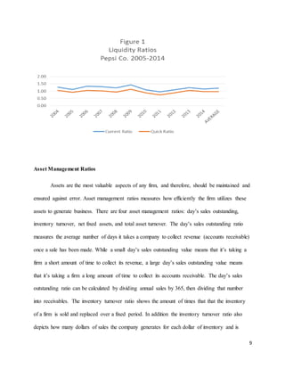
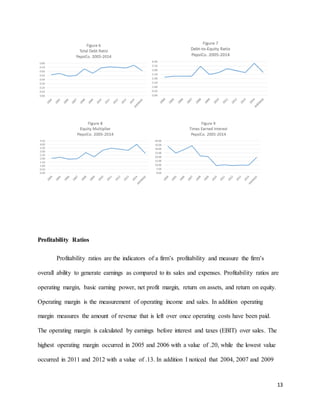
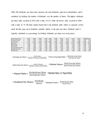
earnings, sales and assets cannot grow any faster than the retained earnings plus the additional
debt that the retained earnings can support.
Assets = Liabilities + Equity
As a result of this assumption requiring that assets equal liabilities plus owners’ equity, any
changes in assets must be equal to changes in liabilities plus changes in owners’ equity.
Δ Assets = Δ Liabilities + Δ Equity
Furthermore, the sustainable growth model assumes that any change in equity can only result
from a change in retained earnings. Therefore, the firm cannot sell additional owners’ equity.
Δ Assets = Δ Liabilities + Δ Retained Earnings
This means the company’s future increase in assets is equal to the future increase in retained
earnings plus the additional debt that is supported by the additional owners’ equity as determined
by the equity multiplier. The equity multiplier is equal to total assets divided by owners’ equity.
Δ Assets = (Δ Retained Earnings) (Equity Multiplier)
[3-10]
An increase in total revenue must be accompanied by a proportionate increase in total assets.
Since any increase in total revenue is limited by the increase in total assets, growth in total
revenue is limited by the increase in retained earnings. Total asset turnover is equal to sales
divided by total assets.

27
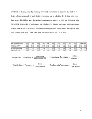
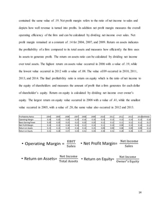
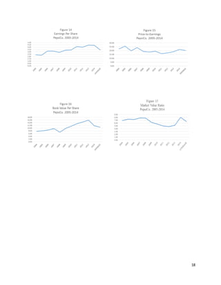
Δ Total Revenue = (Δ Total Assets) (Total Asset Turnover)
[3-11]
The net income required to achieve the target return on equity is determined by total revenue
times the net profit margin. Net profit margin is equal to net income divided by total revenue.
Δ Net Income = (Δ Total Revenue) (Net Profit Margin)
Earnings retention is equal to retained earnings divided by net income.
Earnings Retention = Retained Earnings/Net Income
Sustainable growth is equal to return on equity times the earnings retention rate of the company.
Sustainable Growth = (Return on Equity) (Earnings Retention)
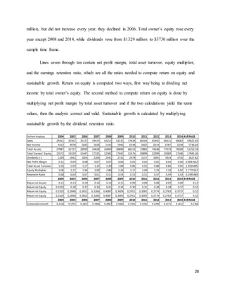
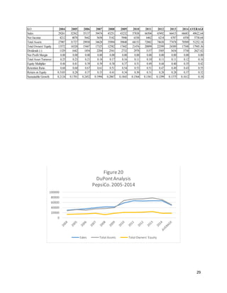
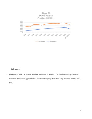
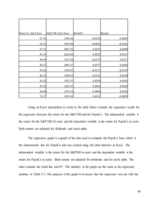
Analysis of ROE and Sustainable Growth for PepsiCo.
The following table contains the data and ratios for the DuPont system of financial
analysis of return on equity as well as the analysis of sustainable growth (G) for PepsiCo based
on data from 2005 to 2014. Lines two through 6 contain the raw data that was used to compute
the ratios used in the DuPont system of financial analysis as well as in the computation of the
sustainable growth rate. From 2004 to 2014, total revenue for PepsiCo increased from $29,261
million to $66,683 million. Total revenue for PepsiCo. Increased every year over the sample time
period except for 2009 due to the nationwide recession. Net income rose from $4,212 million to
$6,558 million over the course of ten years. Total assets rose from $27,987 million to $70,509

28
million, but did not increase every year, they declined in 2006. Total owner’s equity rose every
year except 2008 and 2014, while dividends rose from $1329 million to $3730 million over the
sample time frame.
Lines seven through ten contain net profit margin, total asset turnover, equity multiplier,
and the earnings retention ratio, which are all the ratios needed to compute return on equity and
sustainable growth. Return on equity is computed two ways, first way being to dividing net
income by total owner’s equity. The second method to compute return on equity is done by
multiplying net profit margin by total asset turnover and if the two calculations yield the same
values, then the analysis correct and valid. Sustainable growth is calculated by multiplying
sustainable growth by the dividend retention ratio.

29
KO 2004 2005 2006 2007 2008 2009 2010 2011 2012 2013 2014 AVERAGE
Sales 29261 32562 35137 39474 43251 43232 57838 66504 65492 66415 66683 49622.64
Net Income 4212 4078 5642 5658 5142 5946 6338 6462 6214 6787 6558 5730.64
Total Assets 27987 31727 29930 34628 35994 39848 68153 72882 74638 77478 70509 51252.18
Total Owners' Equity 13572 14320 15447 17325 12582 17442 21476 20899 22399 24389 17548 17945.36
Dividends (-) 1329 1642 1854 2204 2541 2732 2978 3157 3305 3434 3730 2627.82
Net Profit Margin 0.00 0.00 0.00 0.00 0.00 0.00 0.00 0.00 0.00 0.00 0.00 0.00
Total Asset Turnover 0.25 0.23 0.21 0.18 0.17 0.16 0.11 0.10 0.11 0.11 0.12 0.16
Equity Multiplier 0.44 0.41 0.39 0.39 0.38 0.37 0.51 0.49 0.44 0.40 0.35 0.42
Retention Ratio 0.68 0.60 0.67 0.61 0.51 0.54 0.53 0.51 0.47 0.49 0.43 0.55
Return on Equity 0.3103 0.28 0.37 0.33 0.41 0.34 0.30 0.31 0.28 0.28 0.37 0.32
Sustainable Growth 0.2124 0.1701 0.2452 0.1994 0.2067 0.1843 0.1564 0.1581 0.1299 0.1375 0.1612 0.18
0
20000
40000
60000
80000
100000
Figure20
DuPontAnalysis
PepsiCo. 2005-2014
Sales Total Assets Total Owners' Equity

31
References
1. McGowan, Carl B., Jr., John C. Gardner, and Susan E. Moeller. The Fundamentals of Financial
Statement Analysis as Applied to the Coca-Cola Company. New York City: Business Expert, 2015.
Print.

32
Chapter 3: Determining the Long-Term Growth Rate
When valuing a company, both the long-term growth rate and immediate growth rate are
required. Long-term growth rates provide a reflection of the economy as a whole; however, the
possibility of a company growing at an even higher rate than the economy does not last for a
very long time. Eventually, large companies begin to grow at the rate of GDP.
When estimating long term growth for the firm, an estimate of long-term growth for the
entire economy is essential. To do so, the “current dollar” and “real gross domestic product”,
which are published by the U.S. Bureau of Economic Analysis, are needed. Since we are
estimating nominal values, “GDP in billions of current dollars” is used. To estimate long-term
growth rate for PepsiCo, we use the eleven years of GDP. The annual change in GDP, ΔGDP1, is
the difference in GDP from the current year, GDP1, and GDP from the previous year, GDP0,
divided by GDP from the previous year.
The table shows the values for GDP of each year during the period of 2014 to 2004,
along with the changes in GDP for each year. The average change for the entire period was
3.545%. This value is then used in the estimation of long-term growth for PepsiCo.
ΔGDP1= {GDP1- GDP0)/GDP0}

34
-0.04
-0.02
0.00
0.02
0.04
0.06
0.08
2014 2013 2012 2011 2010 2009 2008 2007 2006 2005 2004
Figure21
Change in GDP
Pepsico 2005-2014

35
Chapter 4: Calculating the Beta Coefficientand the Required Rate of Return
for PepsiCo.
Chapter 4 demonstrates how the rate of return is computed for PepsiCo using the modern
portfolio theory with the necessary data downloaded from the internet. It will demonstrate how
to calculate the monthly returns for PepsiCo and the S&P 500 stock Index, then show how to use
the returns to compute the beta co-efficient and the required rate of return. Also shown is how to
validate the data for the market index and company and how to calculate the returns using the
dividends and stock split adjusted prices. Included in this chapter is a demonstration of how to
graph the characteristic line and use the graph to ensure that the regression was run correctly.
Any company can be used, however, in this paper we will evaluate PepsiCo and S&P 500 Index.
This paper can be used as a reference in analyzing PepsiCo for investment purposes.
In 1952 Harry Markowitz created the modern portfolio theory (MPT) which can be used
to explain the relationship between risk and return for assets with specific emphasis on stocks.
In general, when the stock of a company has a high rate of return, the risk associated with it is
usually high and vice versa. Also called "portfolio theory" or "portfolio management theory,"
MPT suggests that it is possible to construct an "efficient frontier" of optimal portfolios, offering
the maximum possible expected return for a given level of risk. It suggests that it is not enough
to look at the expected risk and return of one particular stock. By investing in more than one
stock, an investor can reap the benefits of diversification, particularly a reduction in the amount
of risk of the portfolio. MPT quantifies the benefits of diversification, also known as not putting
all of your eggs in one basket. Non-systematic risk is risk that is particular to a company and
doesn’t affect other companies. Investors can protect against non-systemic risk by diversifying

36
their investments. Non-systemic risk contrasts with systemic risk, which is risk that applies to all
companies in a market or industry. The beta coefficient shows the movement of the returns for
the stock with the market. A higher beta coefficient shows that the return for the stock moves
more than the market (aggressive stocks) and a lower beta coefficient shows that the return
moves less (defensive stocks).
This paper will show how to retrieve the data from the internet for PepsiCo, as well as
how to compute returns for both the market index and the stock, and how to run a regression
analysis to determine the beta coefficient in an attempt to measure the systematic risk of the
stock. A graph displaying the trend line and statistics to verify the first regression is run
correctly (with the correct variable and independent variable) will also be included. All of the
analysis is done using Excel.
All data used for this analysis is downloaded from the EDGAR SEC and the Yahoo
Finance website. Upon arrival to the webpage, the S&P 500 data can be found by clicking on the
“S&P 500” icon, followed by clicking on the “Historical Prices” icon. Click on the monthly
indicator to download monthly data and enter in the dates that are needed. For this, analysis we
downloaded sixty-one monthly observations to calculate sixty monthly returns. The data columns
are: Date, Open, High, Low, Close, Average Volume, and Adjusted Close. The index and the
PepsiCo price are adjusted for splits and dividends. Next, move the cursor to the bottom of the
data and click on “Download to Spreadsheet”. Save the data to a spreadsheet and repeat the
process for the PepsiCo data. Begin by entering the PepsiCo ticker symbol (PEP) and proceed to
download and save the data for the specific time period.

37
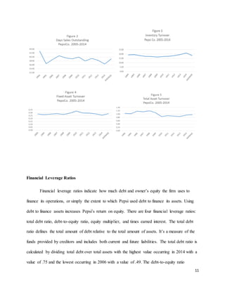
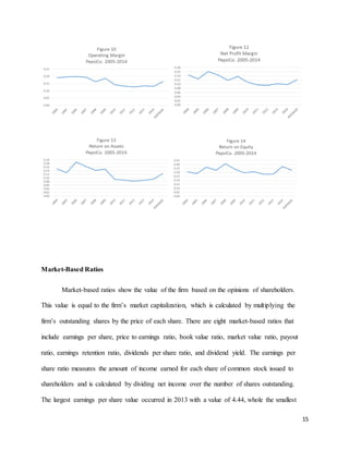
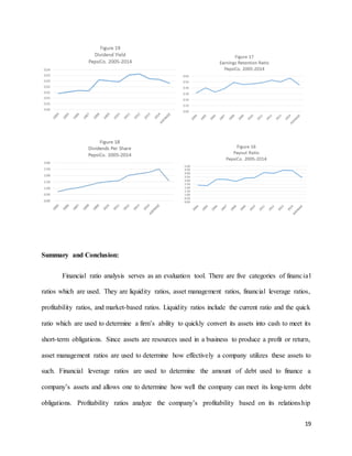
Calculating Returns for the S&P 500 Index and for PepsiCo
To compute the beta coefficient, arithmetic returns are used. Arithmetic returns are
calculated by dividing the ending index or stock value (𝑉𝑎𝑙𝑢𝑒1 ), by the beginning value
(𝑉𝑎𝑙𝑢𝑒0) and subtracting one, as in
Equation [5-1]. An alternative method to calculate the return is to subtract the beginning value
(𝑉𝑎𝑙𝑢𝑒0) from the ending value (𝑉𝑎𝑙𝑢𝑒1 ) and dividing by the beginning value (𝑉𝑎𝑙𝑢𝑒0), as in
Equation [5-2]. Both returns are adjusted for dividends and stock splits. The returns used in the
regression analysis are arithmetic returns.
Return = [(𝑉𝑎𝑙𝑢𝑒1 -𝑉𝑎𝑙𝑢𝑒0) – 1] [5-1]
Return = [(𝑉𝑎𝑙𝑢𝑒1 -𝑉𝑎𝑙𝑢𝑒0)/ 𝑉𝑎𝑙𝑢𝑒0)] [5-2]
Calculating Beta for PepsiCo
The Modern Portfolio Theory illustrates that investors not rewarded for the total risk of
an investment but for the systematic risk. This is because total risk includes those that are firm-
specific and that can be eliminated in a well-diversified portfolio. The regression line between
the monthly returns for the individual security and the market index, which is also the slope
coefficient, shows the specific risk of an individual stock. The coefficient lines are calculated
using a sixty month regression. In this analysis, the beta coefficient for PepsiCo is calculated

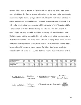
38
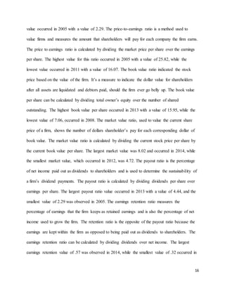
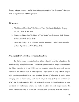
using sixty monthly observations of returns from 01/03/2004 to 01/03/2015 and returns for the
S&P 500 Index for the same time period. Beta is the covariance between returns for PepsiCo and
returns for the S&P 500 divided by the variance for the S&P 500.
𝑅 𝑃𝐸𝑃 = 𝐴𝑙𝑝ℎ𝑎 𝑃𝐸𝑃 + 𝐵𝑒𝑡𝑎 𝑃𝐸𝑃(𝑅 𝑀) [5-3]
Where,
𝑅 𝑃𝐸𝑃 The return for PepsiCo stock
𝐵𝑒𝑡𝑎 𝑃𝐸𝑃 The slope of the regression line between returns for the market and returns for
PepsiCo
𝐴𝑙𝑝ℎ𝑎 𝑃𝐸𝑃 The intercept coefficient for the regression line between returns for the market
and returns for PepsiCo.
𝑅 𝑀 The return on the S&P 500 Stock market Index
(𝑅 𝑀– 𝑅 𝐹) the market risk premium is the additional return that stock holders receive for the
additional risk of holding stocks rather than the risk free asset, long-term
government bonds.
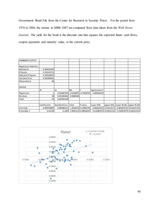
The following table contains the data used to compute the PepsiCo beta and are downloaded
from the yahoo finance website. Column 1 shows the date and Columns 2 and 3 contain the
stock split and dividend adjusted index and price values for the S&P 500 Index and for PepsiCo
stock, respectively. The independent variable is the return for the S&P 500 and the dependent
variable is the return for PepsiCo. The returns are calculated by dividing the ending index or
stock value by the beginning value and subtracting one. An alternative method to calculate the
return is to subtract the beginning value from the ending value and dividing by the beginning

39
value. Both returns are adjusted for dividend and stock splits. The returns used are arithmetic
returns.
In this paper, the CAPM is used to compute the required rate of return for PepsiCo. The
required rate of return for PepsiCo is the minimum rate of return demanded by stockholders of
PepsiCo stock. The model used in this paper is based on the CAPM derived from the work of
Sharpe (1964).
𝑅 𝑃𝐸𝑃 = 𝑅𝑓 + 𝐵𝑒𝑡𝑎 𝑃𝐸𝑃 (𝑅 𝑚 – 𝑅 𝐹)
[5-4]
𝑅 𝑃𝐸𝑃 = the required rate of return for PepsiCo Stock
𝑅𝑓 = the risk free rate of return
𝐵𝑒𝑡𝑎 𝑃𝐸𝑃= the beta coefficient for PepsiCo
𝑅 𝑚= the rate of return on the stock market
(𝑅 𝑚 – 𝑅 𝐹) = the market risk premium
The required rate of return for PepsiCo is the risk-free rate of return plus the risk
premium. The risk premium is the beta for PepsiCo times the market price of risk.

40
Using an Excel spreadsheet to create it, the table below contains the regression results for
the regression between the return for the S&P 500 and for PepsiCo. The independent variable is
the return for the S&P 500 (X-axis) and the dependent variable is the return for PepsiCo (y-axis).
Both returns are adjusted for dividends and stock splits.
The regression graph is a graph of the data used to compute the PepsiCo beta, which is
the characteristic line for PepsiCo and was created using the chart function in Excel. The
independent variable is the return for the S&P500 (x-axis) and the dependent variable is the
return for PepsiCo (y-axis). Both returns are adjusted for dividends and for stock splits. The
chart contains the trend line and 𝑅2
. The statistics in the graph are the same as the regression
statistics in Table 5-1. The purpose of the graph is to ensure that the regression was run with the

41
correct independent and dependent variable. If the trend line and statistics in the graph are not
identical to the numbers in the regression, the variables may have been reversed.
Calculating the Required Rate of Return for Stocks
In this paper, the CAPM is used to compute the required rate of return for PepsiCo. The
required rate of return for PepsiCo is the minimum rate of return demanded by stockholders of
PepsiCo stock. The model used in this paper is based on the CAPM derived from the work of
William F. Sharpe (1964).
𝑅 𝑃𝐸𝑃 = 𝑅𝑓 + 𝐵𝑒𝑡𝑎 𝑃𝐸𝑃 (𝑅 𝑚 – 𝑅 𝐹)
[5-4]
𝑅 𝑃𝐸𝑃 = the required rate of return for PepsiCo Stock
𝑅𝑓 = the risk free rate of return
𝐵𝑒𝑡𝑎 𝑃𝐸𝑃= the beta coefficient for PepsiCo
𝑅 𝑚= the rate of return on the stock market
(𝑅 𝑚 – 𝑅 𝐹) = the market risk premium
The required rate of return for PepsiCo is the risk-free rate of return plus the risk
premium. The risk premium is the beta for PepsiCo times the market price of risk.
Calculating the Required Rate Return for PepsiCo Using the CAPM
The risk free rate is the total return (income plus capital appreciation) on Long-term
Government Bonds taken from SBBI 2007. For the years from 1926 to 1976, SBBI used the

42
Government Bond File from the Center for Research in Security Prices. For the period from
1976 to 2006, the returns in SBBI 2007 are computed from data taken from the Wall Street
Journal. The yield for the bond is the discount rate that equates the expected future cash flows,
coupon payments and maturity value, to the current price.
SUMMARY OUTPUT
Regression Statistics
Multiple R 0.464910476
R Square 0.216141751
Adjusted R Square 0.202626953
Standard Error 0.030304661
Observations 60
ANOVA
df SS MS F Significance F
Regression 1 0.014687503 0.0146875 15.9929701 0.000182247
Residual 58 0.053265602 0.0009184
Total 59 0.067953106
Coefficients Standard Error t Stat P-value Lower 95% Upper 95% Lower 95.0% Upper 95.0%
Intercept 0.005970085 0.004082312 1.4624274 0.14902192 -0.002201551 0.01414172 -0.002201551 0.014141721
X Variable 1 0.42139 0.1054 3.9991212 0.00018225 0.210467675 0.63231212 0.210467675 0.632312122

43
References
1. McGowan, Carl B., Jr. Corporate Valuation Using the Free Cash Flow Method Applied
to Coca-Cola. N.p.: n.p., n.d. Print.
Chapter 5: Free CashFlow to Equity
Corporate financial management is used to maximize the value of the firm, where, the
value of the firm is measured by the market capitalization of the company. The market
capitalization of the company is calculated by multiplying the total number of shares outstanding
by the market price per share. The value of the company is also determined by the risk and return
characteristics of the company which is determined by the decisions of the corporate financial
managers. Therefore, a company that has a goal of higher rates of return would assume higher
risk responsibilities and invest in an industry such as oil fracking. Similarly, a company that
takes lower risks would be forced to accept lower rates of returns and invest in an industry like
money market management such as T bills.
Decisions made by financial managers fall under three categories: investment decisions,
financing decisions and dividend decisions. Investment decisions determine the types of assets
that should be purchased and directly impacts the relationship between current assets and fixed
assets. Higher ratios of current assets to fixed show less risk of default or insolvency. Lower
return on assets and return on equity results from a high current ratio. Financing decisions are
related to how the company uses fixed cost sources of funding (i.e. long-term bonds). The greater
the financial leverage of a company, the higher the returns on equity are expected to be. The

44
dividend decision involves the allocation of funds; even though it is not an asset decision, it does
affect the financial leverage.
The distribution of future cash flows, which is a decision maker’s estimate, is based on
accounting information that is provided by financial managers. The probability distribution of
expected cash flows is used to determine the total market capitalization (value) of the company.
Higher expected cash flows along with lower required rates of return equate to a higher value
company.
Valuing a Share of Stock Using the Free Cash Flow Model
A stock’s value is determined by the future free cash flow to equity (FCFE).
𝑃0= 𝐹𝐶𝐹𝐸1 + 𝐹𝐶𝐹𝐸2 + 𝐹𝐶𝐹𝐸3 + …….. [6-1]
However, since the Free Cash Flow to Equity is in the future, each Free Cash Flow to Equity
must be discounted to the present time by the cost of equity (k).
Therefore,
𝑃0=
𝐹𝐶𝐹𝐸1
(1+𝑘)1 +
𝐹𝐶𝐹𝐸2
(1+𝑘)2 +
𝐹𝐶𝐹𝐸3
(1+𝑘)3 + ……… [6-2]
The discounted present value of the future stream of Free Cash Flow to Equity discounted at the
cost of equity can be represented as: the sum of each Free Cash Flow to Equity (𝐹𝐶𝐹𝐸𝑡)
discounted by one, plus the cost of equity (1 + 𝑘 ) 𝑡
, from time zero to time infinity.
𝑃0 =  𝐹𝐶𝐹𝐸𝑡/(1 + 𝑘 ) 𝑡
[6-3]

45
If we assume that the future Free Cash Flow to Equity will grow at a constant rate (g), each
future Free Cash Flow to Equity is equal to the Free Cash Flow to Equity at time zero times one,
plus the growth rate raised to the power of t. 𝐹𝐶𝐹𝐸𝑡 = 𝐹𝐶𝐹𝐸0 (1 + 𝑔 ) 𝑡
. We can substitute this
value of 𝐹𝐶𝐹𝐸𝑡 into formula [6-3].
𝑃0 = 𝐹𝐶𝐹𝐸0 (1 + 𝑔 ) 𝑡
/ (1 + 𝑘 ) 𝑡
[6-4]
If g and k are constant and k is strictly greater than g, Equation [6-4] can be simplified to
Equation [6-5]. That is, the value of an investment is equal to the anticipated Free Cash Flow to
Equity at time t=1 discounted at the cost of equity minus the growth rate.
𝑃0 = 𝐹𝐶𝐹𝐸1/ (k - g) [6-5]
That is the value of a share of stock in the firm is equal to the anticipated future dividend divided
by the required rate of return for equity minus the expected future growth rate of FCFE for the
firm. This model assumes that FCFE will be greater than zero and that k is strictly greater than g.
The Super-Normal Growth Model
The super-normal growth period is the time period where the growth rate will be above
average. After the super-normal growth period, the growth of the company returns to the long-
term growth rate of the economy (based on the GDP). The present value of the shares in the firm
is equal to the discounted present value of the Free Cash Flow to Equity ( 𝐹𝐶𝐹𝐸𝑡) for the super-
normal growth period, plus the present value of the future Free Cash Flow to Equity for the
normal growth period. The practice for company valuations is to compute five years of super-
normal growth and then assume a constant long-term growth rate.

46
𝑃0 =
𝐹𝐶𝐹𝐸1
(1+𝑘)1 +
𝐹𝐶𝐹𝐸2
(1+𝑘)2 +
𝐹𝐶𝐹𝐸3
(1+𝑘)3 +
𝐹𝐶𝐹𝐸4
(1+𝑘)4 +
𝐹𝐶𝐹𝐸5
(1+𝑘)5 +
𝑃5
(1+𝑘)5 [6-
6]
The Free Cash Flow to Equity values for years 1 to 5 are computed using the super
normal growth rate ( g*) and the Free Cash Flow to Equity for year six is computed using the
long-term normal growth rate,(g). 𝐹𝐶𝐹𝐸1 is equal to the value of 𝐹𝐶𝐹𝐸0 times the growth
factor [ 𝐹𝐶𝐹𝐸0(1 + 𝑔 ∗)1
]. 𝐹𝐶𝐹𝐸2 is equal to the value of 𝐹𝐶𝐹𝐸1 times the growth factor
[ 𝐹𝐶𝐹𝐸1(1+ 𝑔 ∗)1
]. The rest of the Free Cash Flow to Equity values until 𝐹𝐶𝐹𝐸5 are computed
using the super-normal growth rate. 𝐹𝐶𝐹𝐸6 is equal to the value of 𝐹𝐶𝐹𝐸5 times the normal
growth rate, 𝐹𝐶𝐹𝐸5 (1 + 𝑔)1
.
𝐹𝐶𝐹𝐸1 = 𝐹𝐶𝐹𝐸0(1 + 𝑔 ∗)1
[6-7]
𝐹𝐶𝐹𝐸2 = 𝐹𝐶𝐹𝐸1(1 + 𝑔 ∗)1
[6-8]
𝐹𝐶𝐹𝐸3 = 𝐹𝐶𝐹𝐸2(1+ 𝑔 ∗)1
[6-9]
[6-10]
[6-11]
𝐹𝐶𝐹𝐸6 = 𝐹𝐶𝐹𝐸5(1+ 𝑔)1
[6-12]
After time = 5, it is assumed that the firm will return to a normal long term growth rate that is
constant. The terminal value of the investment at time = 5 is the discounted present value of all
of the future Free Cash Flow to Equity, beginning with Free Cash Flow to Equity six. The
terminal value ( 𝑃5) is equal to the discounted present value of all of the future FCFE. Beginning
with 𝐹𝐶𝐹𝐸6, the future cash flows are assumed to grow at a constant rate (g).

47
𝑃5 = 𝐹𝐶𝐹𝐸6 / (k-g) [6-13]
After the future Free Cash Flow to Equity values are computed for years one to five and the
terminal value at time five is computed, each cash flow is discounted to the present time (t=0).
The future cash flows are discounted at the cost of equity (k), and discounted for the number of
years in the future that the cash flow will be received.
𝑃𝑉 (𝐹𝐶𝐹𝐸1) = 𝐹𝐶𝐹𝐸1(1+ 𝑘)1
[6-14]
𝑃𝑉 (𝐹𝐶𝐹𝐸2) = 𝐹𝐶𝐹𝐸2(1 + 𝑘)2
[6-15]
[6-16]
[6-17]
[6-18]
𝑃𝑉 (𝑃5) = 𝑃5/(1+ 𝑘)5
[6-19]
Hence, the present value of the investment is equal to the sum of the six present values of the
future Free Cash Flow to Equity and the future terminal value.
𝑃0 = 𝑃𝑉 (𝐹𝐶𝐹𝐸1) + 𝑃𝑉 (𝐹𝐶𝐹𝐸2) + 𝑃𝑉 (𝐹𝐶𝐹𝐸3) + 𝑃𝑉 (𝐹𝐶𝐹𝐸4) + 𝑃𝑉 (𝐹𝐶𝐹𝐸5) + 𝑃𝑉 (𝑃5)
Free Cash Flow to Equity
In this analysis, the super-normal growth rate model is combined with the free cash flow
to equity model. In the FCFE model, FCFE is defined as net income minus net capital
expenditures minus the change in working capital plus net changes in the long-term debt
position. Net income is taken from the income statement. Net capital expenditure equals capital

48
expenditures minus depreciation; and are both derived from the statement of cash flows. The
change in working capital is the difference of accounts receivable plus inventory from one year
to the next minus the difference in accounts payable from one year to the next.
Therefore,
FCFE = NI – (CE-D) – (Δ WC) + (NDI-DR) [6-21]
Where,
FCFE Free Cash Flow to Equity
(CE-D) Net Capital Expenditures
(Δ WC) Changes in non-cash working capital accounts: accounts receivable, inventory,
payables
(NDI-DR) New debt issues are a cash inflow while the repayment of outstanding debt is a
cash outflow. The difference is the net effect of debt financing on cash flow.
NI Net Income
CE Capital Expenditure
D Depreciation
Δ WC Change in Working Capital
NDI New Debt Issued
DR Debt Retired

49
Computing Free Cash Flow to Equity for PepsiCo (2005-2014)
Table 1 shows the computation of FCFE for PepsiCo for the period of 2005 to 2014.
This was done using the data from PepsiCo’s 10-K forms for the time periods. Net income was
derived from the income statement. Capital expenditure is the difference between purchases of
Property, Plant and Equipment and Depreciation taken from the Statement of Cash Flows). The
change in working capital for each year is calculated by taking the difference in each of the
working capital accounts for each year from 2005 to 2014. Working capital accounts include
accounts receivable, inventory, and accounts payable. The change in working capital is defined
as the net change in accounts receivable plus inventory minus accounts payable. When net
income, depreciation, capital expenditure and the change in working capital are combined we
have FCFE before changes in debt. Net cash flow from debt equals new debt financing minus old
debt retirement, which is added to FCFE before debt to compute FCFE after debt.
Table 1

50
Year NI Dep Cap Exp
Change
(WC) FCFE(BD) NCFTD FCFE(AD)
2005 4,078 1,308 -1,648 404 4,142 -152 3,990
2006 5,642 1,406 -2,019 -172 4,857 -106 4,751
2007 5,658 1,426 -2,383 78 4,779 1589 6,368
2008 5,142 1,543 -2,070 145 4,760 831 5,591
2009 5,946 1,635 -2,348 -183 5,083 3070 8,153
2010 6,338 2,327 -3,172 343 5,836 5892 11,728
2011 6,462 2,737 -3,255 -210 5,734 633 6,367
2012 6,214 2,689 -2,619 263 6,547 3500 10,047
2013 6,787 2,663 -2,686 909 7,673 301 7,974
2014 6,558 2,625 -2,744 1032 7,491 1666 9,157
Avg 7,413
Chapter 6: Valuing PepsiCo
This chapter of the analysis illustrates how calculations were done to determine Free Cash Flow
to Equity for PepsiCo. It was done using the input data collected from Chapter 3 to Chapter 5.
Column 1 Year for which FCFE is estimated from 2015 to 2020
Column 2 Projected Free Cash Flow to Equity for years 2015 to 2020 (assuming a
growth rate of 18.76% from Chapter 3

51
Column 3 Present Value of FCFE for years 2015 to 2020 discounted at the required
rate of return for equity for PepsiCo of 4.95%
When we value a stock that has a period of super-normal growth, that value of the equity
is the discounted present value of the expected free cash flow to equity during the super-normal
growth period plus the terminal value of the stock at the end of the super-normal growth period.
In valuing PepsiCo, it is assumed that the super-normal growth period will last five years. This
is standard in the valuation industry because projections beyond five years are very uncertain.
The value of the stock at the end of the super-normal growth period is the discounted present
value of all of the future free cash flow to equity and is computed from the 𝑃5= 𝐹𝐶𝐹𝐸6/ (k-g).
The difference is that the present value of a share of stock at time=t is equal to the anticipated
free cash flow to equity at time= (t+1). Beginning with time= (t+1), the investment returns to the
long-term growth rate with both (k) and (g) becoming constant and (k) being strictly greater than
PEP 8.49%
g(GDP) 3.55%
(k-g) 4.95%
g* 0.1786
Year FCFE PV(FCFE)
Average 7,413
2015 8736 8053
2016 10297 8748
2017 12136 9503
2018 14303 10324
2019 16858 11216
2020 352884 277199
Total 325043

52
(g). Since we are using a super-normal growth period of five years, the terminal value of the
stock is
𝑃5= 𝐹𝐶𝐹𝐸6/ (k-g). The value of it is five years into the future and must be discounted to the
present using the cost of equity.
Conclusion
In this analysis, the concepts of equity valuation, super-normal growth, required rate of
return on equity and sustainable growth were combined to determine the market value of
PepsiCo (PEP). The value of the equity of a firm is defined as the present value of all future cash
flows from the firm to the shareholders. The value of the firm is FCFE divided by the sum of the
required rate of return for equity minus the growth rate of the firm’s earnings. Free Cash Flow to
Equity is defined as net income minus net capital expenditures minus the change in net working
capital plus the net change in long-term debt financing. The required rate of return for equity is
computed using the CAPM using a five-year monthly rate of return beta relative to the S&P 500
Index. Sustainable growth for the super-normal growth period is computed with the extended
DuPont model. The long-term growth rate is assumed to be the same as the growth rate of the
economy.

53
Works Cited
"The History of Pepsi-Cola." The History of Pepsi-Cola. Leader Distribution Systems, Inc., 2012. Web.
20 Oct. 2015.
"Journey: A Glimpse Into The History of Pepsi Bottles." Bottle Bonanza. Bottle Bonanza, 28 Nov.
2010. Web. 20 Oct. 2015.
McGowan, Carl B., Jr. Corporate Valuation Using the Free Cash Flow Method Applied to Coca-Cola.
N.p.: n.p., n.d. Print.
McGowan, Carl B., Jr., John C. Gardner, and Susan E. Moeller. The Fundamentals of Financial
Statement Analysis as Applied to the Coca-Cola Company. New York City: Business Expert,
2015. Print.
"Pepsi Store - History of the Birthplace of Pepsi." Pepsi Store - History of the Birthplace of Pepsi.
Pepsi Store, n.d. Web. 20 Oct. 2015.

Financial Analysis Text

Recommended

Recommended

More Related Content

What's hot

What's hot (20)

Similar to Financial Analysis Text

Similar to Financial Analysis Text (20)

Financial Analysis Text