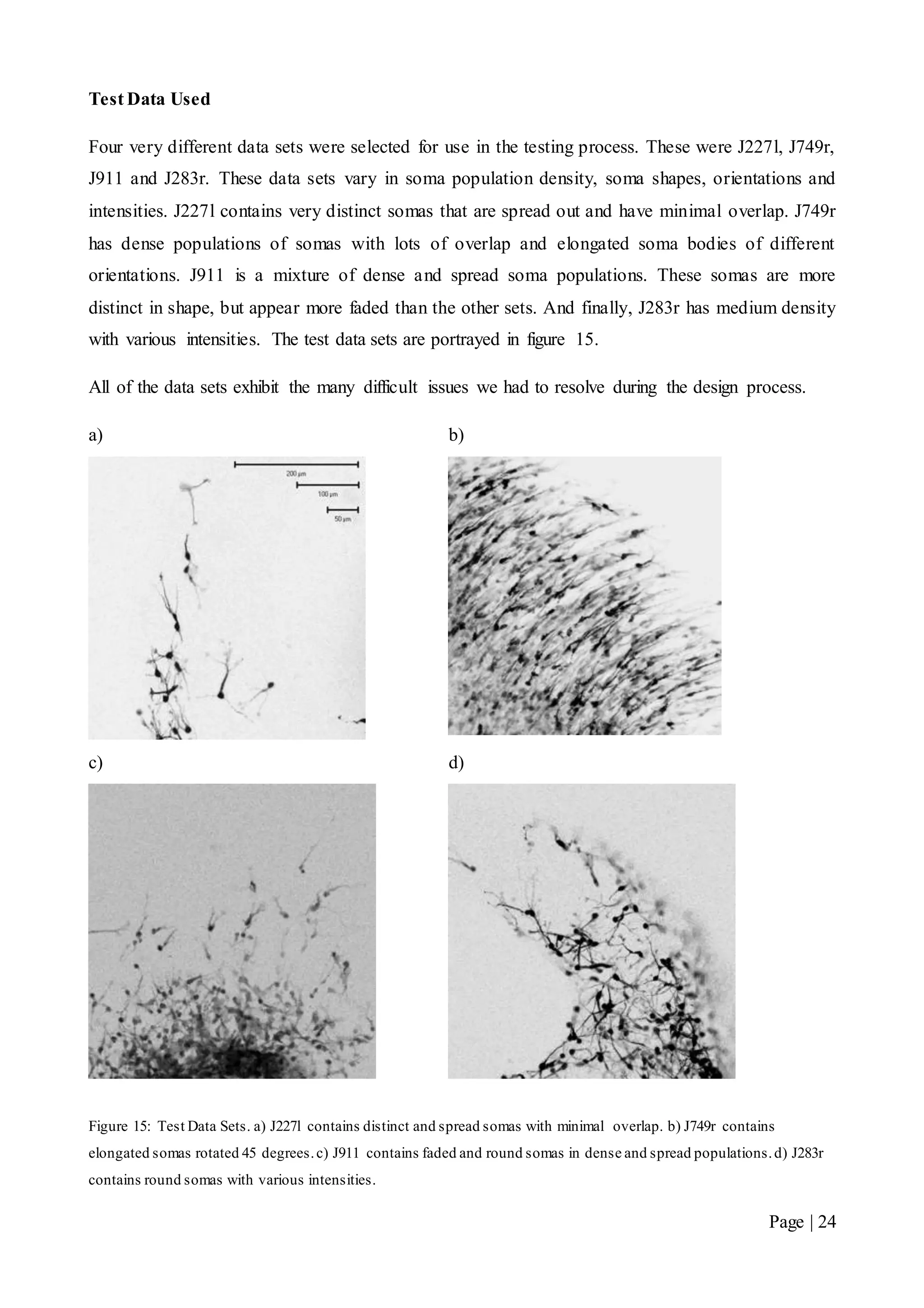
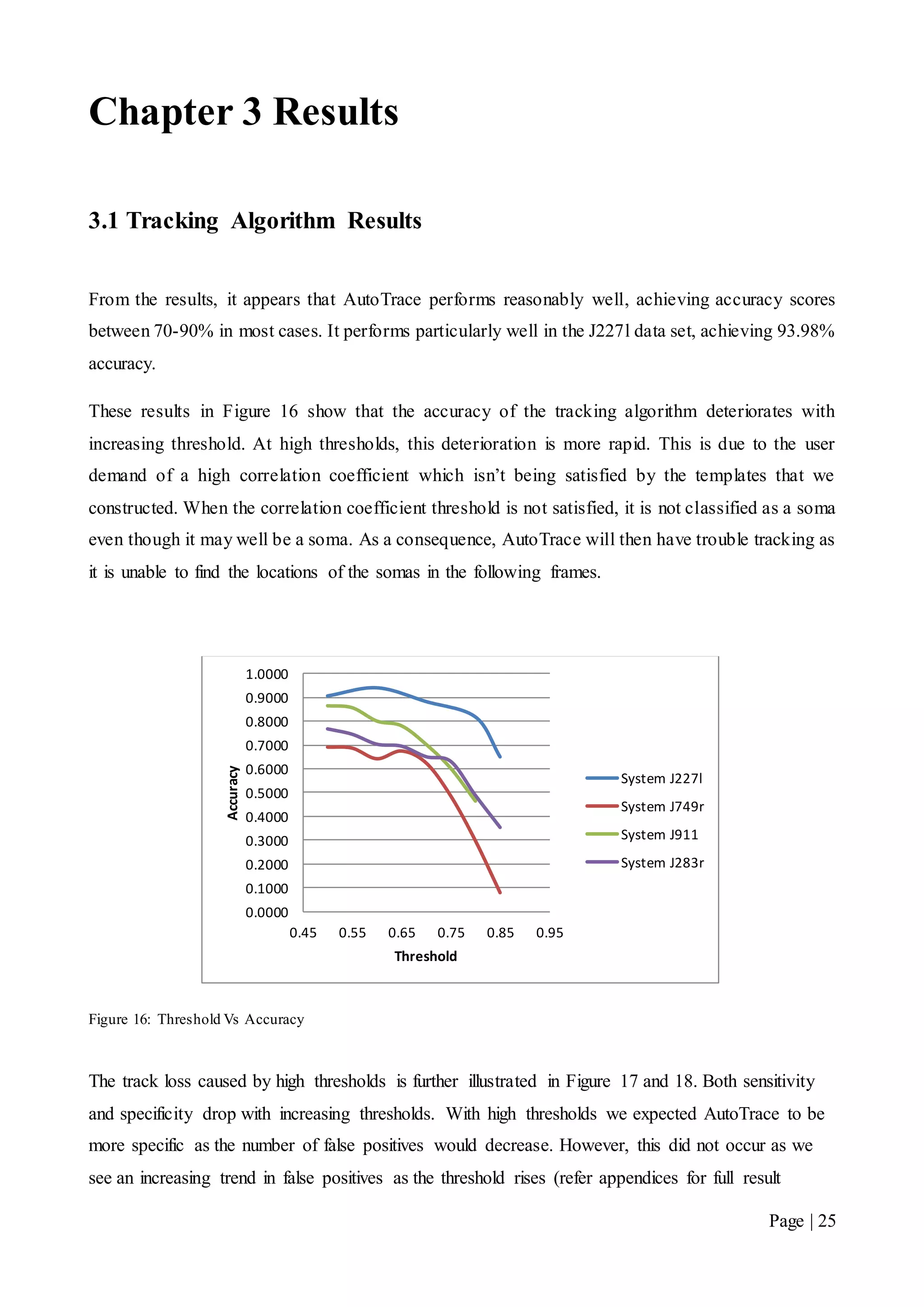
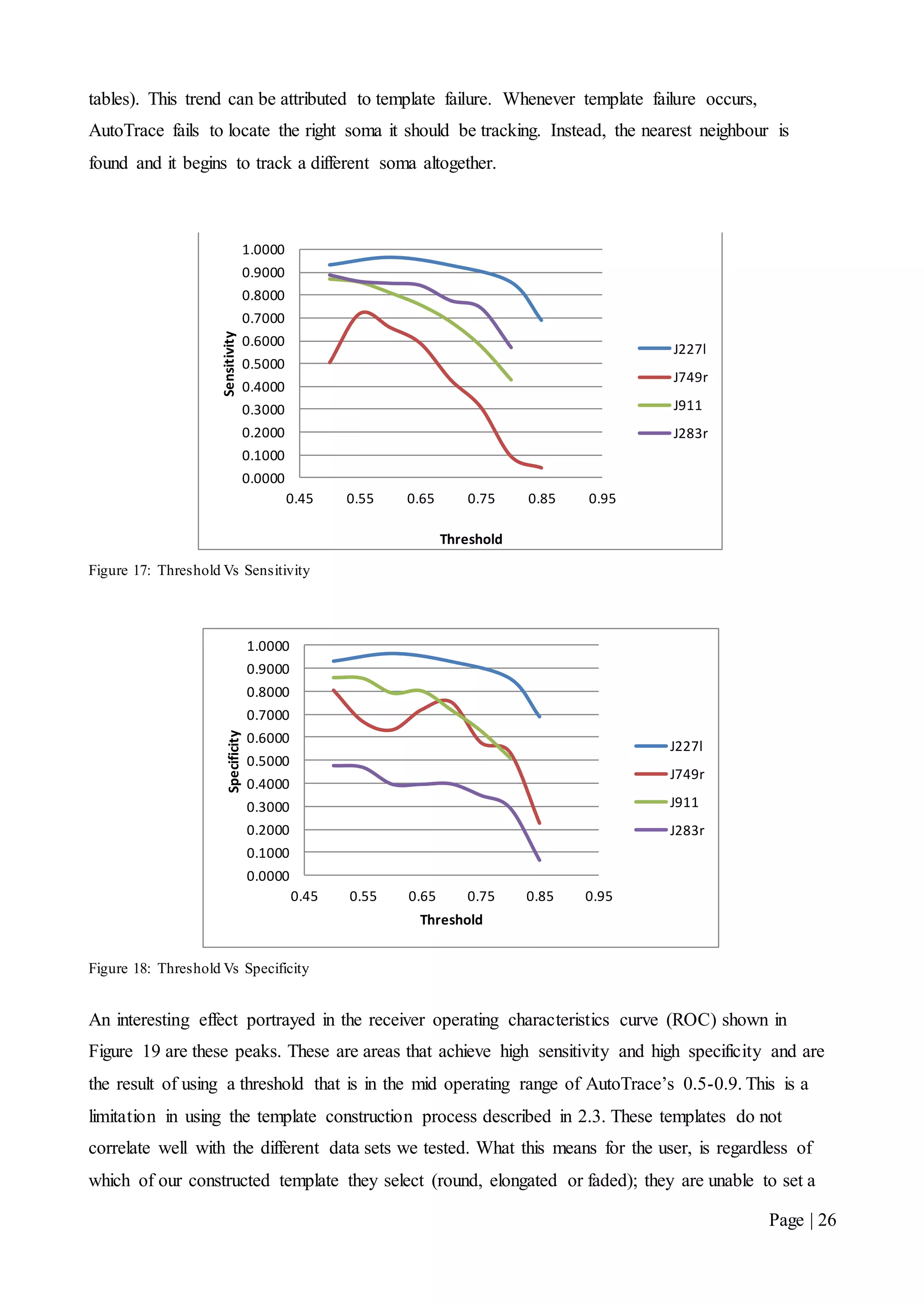
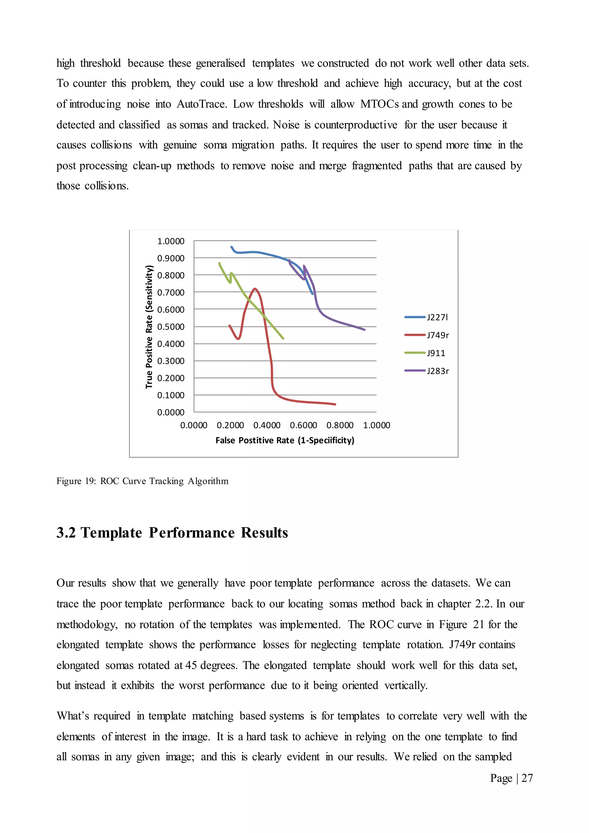
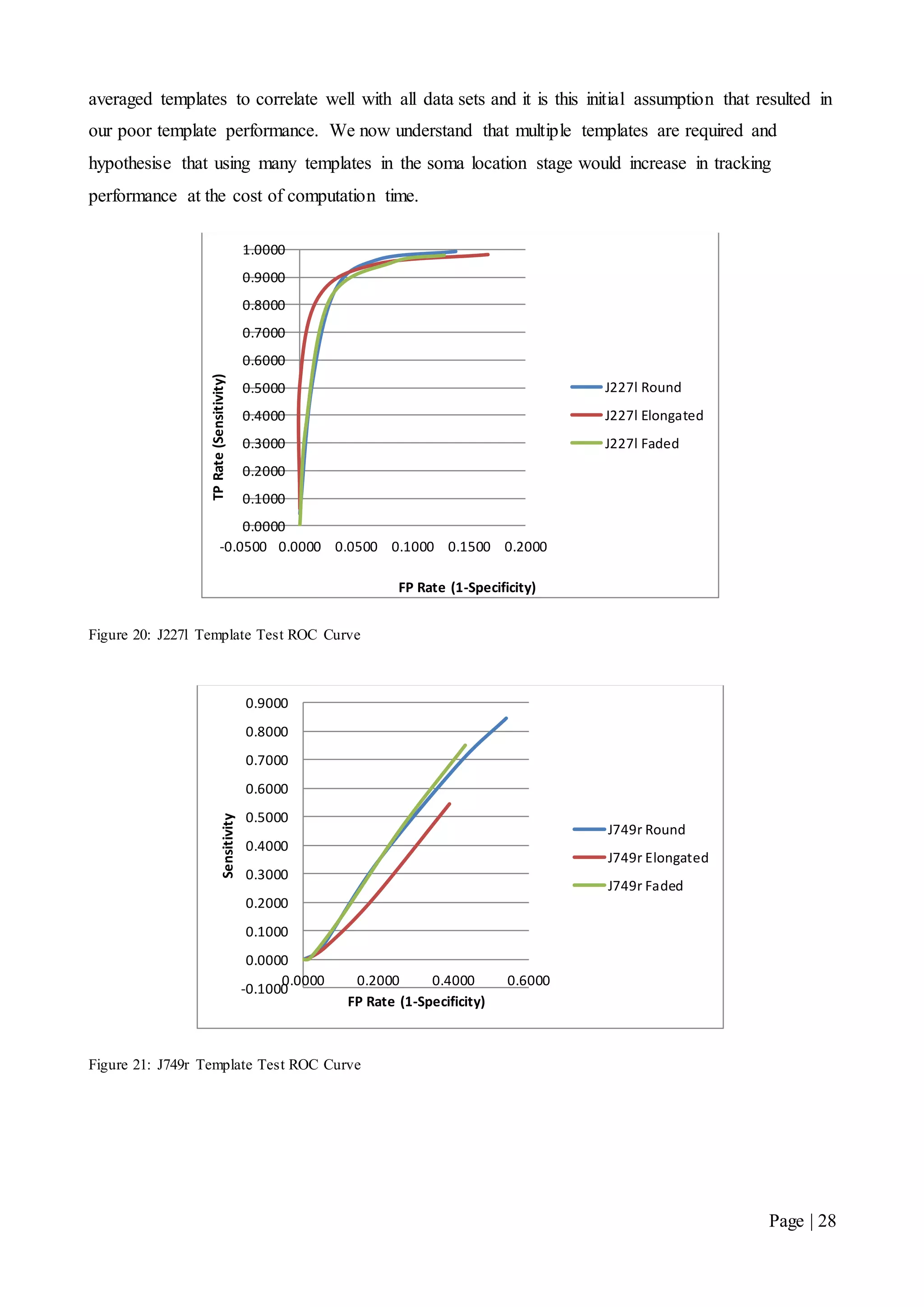
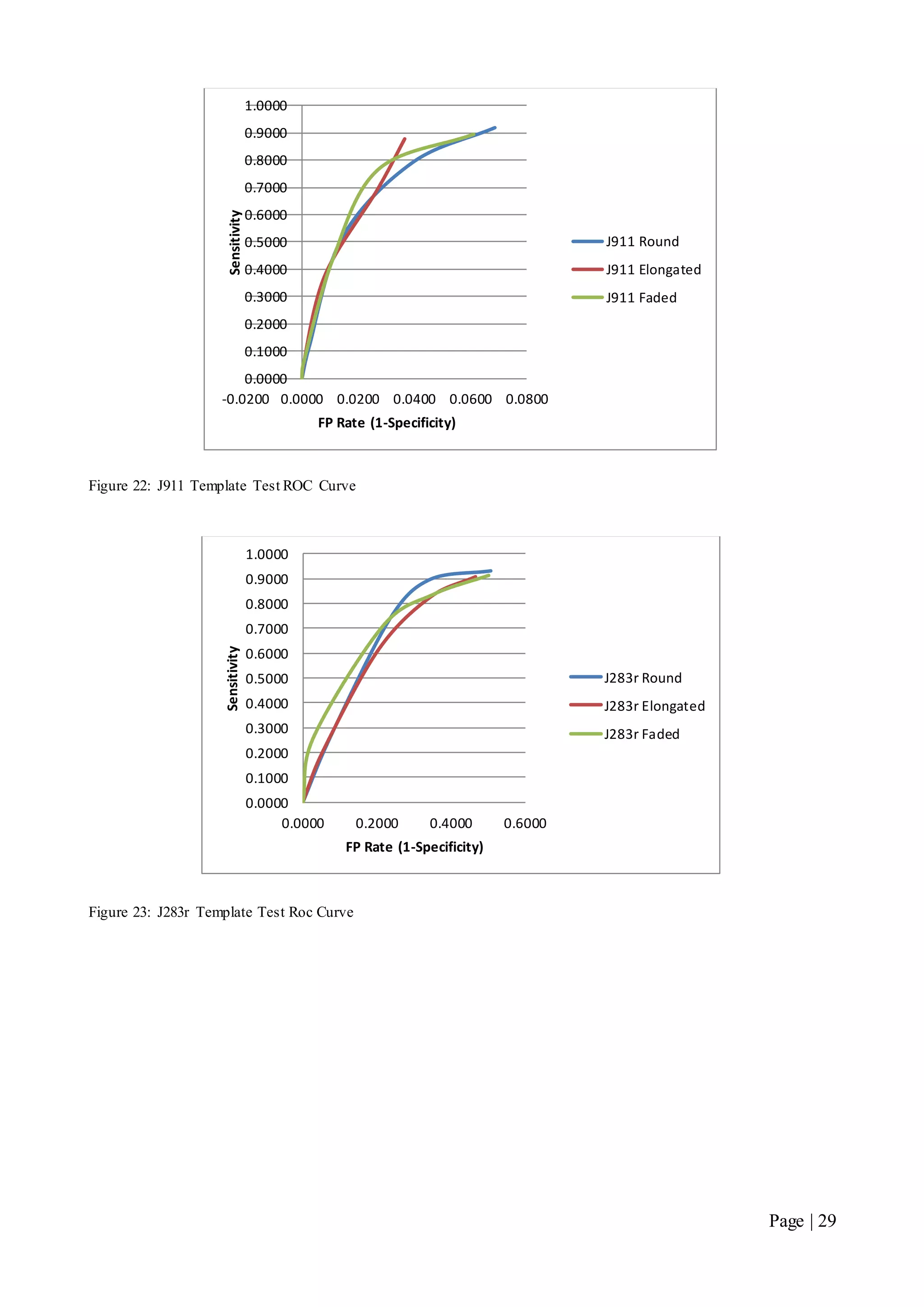
Final Year Project Report Candidate 3

DEPARTMENT OF ELECTRICAL & ELECTRONIC
ENGINEERING
FINAL YEAR PROJECT
LJ2: TRACKING NEURON MIGRATION
Authors: Supervisor:
Simon TIEN 267982 Dr. Leigh JOHNSTON
Leo Zhang 268386
Final Report
October 25, 2011

Page | I
Declaration
The work in this thesis was performed under the supervision of Dr. Leigh Johnston in the
Department of Electrical and Electronic Engineering at the University of Melbourne.
I declare that
i) the report comprises only our original work,
ii) due acknowledgement has been made in the text to all other material used,
iii) the report is less than 60 pages in length, exclusive of tables, maps, bibliographies and
appendices.
iv) Both students contributed equally to all areas of this project
Simon Tien & Leo Zhang
October 2011

Page | II
Acknowledgements
We are very grateful to our supervisor Dr. Leigh Johnston for her guidance and supervision
throughout the year.
We would also like to thank Dr. Joanne Britto from the Howard Florey Institute for her advice in
regards to user implementation, as well as providing us with additional support materials.
Finally we would like to thank the staff at The Department of Electrical and Electronic Engineering
for their support and guidance in writing this report.

Page | III
Abstract
Neuroscientists who study the embryonic brain are interested in how neurons follow migratory
paths from their places of origin to their final destinations. The tracking of these neuronal migratory
routes is of key importance in the study of developmental processes and disorders. Currently,
Neuroscientists tag these neurons manually on a sequence of images. However, this is a long and
tedious process and is very unproductive. This project considers the problem of automating the
neuron tracking procedure by using pattern recognition algorithms.
The tracking system is based on MATLAB’s image processing suite and building on the previous
program AutoTrace. By using a simple method of correlating an image of a soma with each frame
in the sequence, we were able to locate neurons with a degree of accuracy. Applying a simple
nearest neighbour algorithm allowed each neuron’s migratory path to be tracked over the whole
image sequence.
The many challenges of automating the neuron tracking procedure were met with various strategies.
Testing was done to establish the accuracy of the algorithms implemented and results show a
balance between accuracy and the number of false positive errors.

Page | IV
Symbols and Terms
We will use the following terms in our report:
Frame: one image in a time series of neurons of the embryonic brain.
Frame Sequence: a set of frames taken at discrete time intervals.
Template: an image of a soma to be convolved with a frame image.
Soma: The cell body or nucleus of a neuron that we are interested in tracking the migration paths of.
MTOC: Microtubule Organising Centre of a neuron. These provide structural support and assist in
cellular transport. They appear like somas in our datasets, only much smaller in size. MTOCs are
considered to be undesirable noise in our system.
Axon: A fibre branch connecting the soma to the growth cone.
Growth Cone: The tip of an axon. Growth cones explore the cellular environment and determine
the direction of growth, guiding the axon into that direction. These also appear like somas in our
datasets, only much smaller in size.
MATLAB: Numerical computing software that has efficient matrix processing and supports the
building of user interfaces. This software suite serves as the foundation for all our implemented
algorithms.
Migration path: A set of coordinates describing the location of one soma within a frame sequence.

Page | V
Contents
Chapter 1 Introduction.........................................................................................................................1
1.1 Background................................................................................................................................1
1.2 Review of Existing Cell Tracking Software..............................................................................4
1.3 AutoTrace ..................................................................................................................................6
1.4 Document Structure...................................................................................................................6
Chapter 2 Design and Development ....................................................................................................7
2.1 Convolution in Imaging .............................................................................................................7
2.2 Locating Somas..........................................................................................................................8
2.3 Constructing a Soma Template................................................................................................10
2.4 Tracking Somas........................................................................................................................13
2.5 Detection of New Somas..........................................................................................................14
2.6 Track Loss and Control............................................................................................................15
2.7 Testing Procedure ....................................................................................................................21
Chapter 3 Results ...............................................................................................................................25
3.1 Tracking Algorithm Results.....................................................................................................25
3.2 Template Performance Results ................................................................................................27
Chapter 4 Conclusion.........................................................................................................................30
4.1 Overview..................................................................................................................................30
4.2 General Scope and Future Work..............................................................................................30
Bibliography.......................................................................................................................................32
Appendices.........................................................................................................................................33
A: Tables of Results.......................................................................................................................33
B: AutoTraceV41 Guide ................................................................................................................37
B1: Getting Started.....................................................................................................................37
B2: Using AutoTrace .................................................................................................................38
B3: Merging Paths .....................................................................................................................41
B4: Quick Delete........................................................................................................................42
B5: Loading Saved Data ............................................................................................................43
B6: Replicating Test Results......................................................................................................45

Page | VI
List of Figures
Figure 1: The Basic Structure of a Neuron ................................................................................1
Figure 2: An image of immature neurons found in the embryonic brain of mice .....................3
Figure 3: An image of a typical immature neuron. ....................................................................4
Figure 4: Visualisation of two dimensional convolution. ..........................................................8
Figure 5: Correlation coefficients scale and meaning in soma location ....................................9
Figure 6: Correlation matrix thresholding illustration.. .............................................................9
Figure 7: The features of a neuron that appear on a frame ......................................................10
Figure 8: Four elongated soma samples and their averaged template. ....................................12
Figure 9: Constructed templates for AutoTrace's soma detection ...........................................12
Figure 10: Soma Movement Distances per Frame System J249r and System J227l...............14
Figure 11: How a new soma coordinate is recognized by AutoTrace. ....................................15
Figure 12: Soma Collision Illustration.....................................................................................16
Figure 13: Flowchart of tracking algorithm.............................................................................20
Figure 14: Tracking Algorithm Test Procedure .......................................................................23
Figure 15: Test Data Sets.........................................................................................................24
Figure 16: Threshold Vs Accuracy ..........................................................................................25
Figure 17: Threshold Vs Sensitivity ........................................................................................26
Figure 18: Threshold Vs Specificity ........................................................................................26
Figure 19: ROC Curve Tracking Algorithm............................................................................27
Figure 20: J227l Template Test ROC Curve ...........................................................................28
Figure 21: J749r Template Test ROC Curve ...........................................................................28
Figure 22: J911 Template Test ROC Curve ............................................................................29
Figure 23: J283r Template Test Roc Curve .............................................................................29

Page | 1
Chapter 1 Introduction
An important field of research in neuroscience is brain development and regeneration. Scientists are
interested in how newly born neurons are assembled, connected, and how they migrate from their
birthplace to their final resting locations in the brain. The study of neuron migration paths aids
scientists in understanding how defects in brain development can occur. Defects in neuronal
migration development can lead to cognitive, motor, and intellectual disability, as well
as neurological disorders such as autism, Rett syndrome, and mental retardation.
1.1 Background
1.1.1 Immature Neurons and Brain Development
Neuron cells are biological cells found in most animals and are the core components of the nervous
system that includes the brain and the spinal cord. It is an electrically excitable cell that processes
and transmits information by electrical and chemical signalling. Neurons are diverse in category
and a number of specialized types of neurons exist. However, let us begin with a description of the
structure and function of a typical neuron.
Figure 1: The Basic Structure of a Neuron
Source:http://www.ncbi.nlm.nih.gov/books/NBK10064/bin/ch12f22.jpg
Shown in Figure 1, the main features of a typical neuron are the cell body (commonly referred as
the ‘soma’), the growth cone, the axon and the dendrites. The soma is considered as the nucleus of a

Page | 2
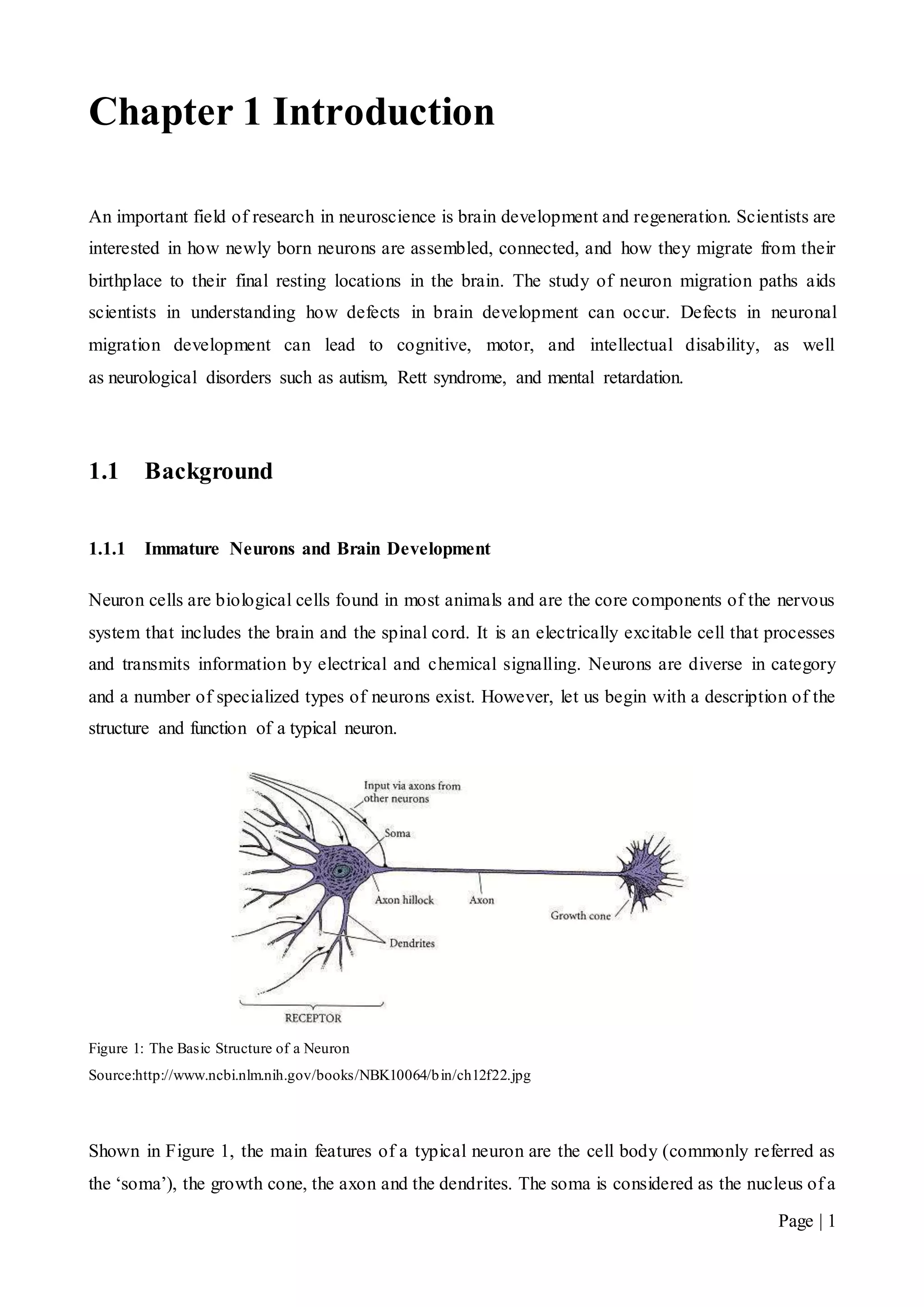
neuron and has the responsibility of maintaining the cell functionality. The growth cone explores
the cellular environment, determining the direction of growth and guides the axon to that direction.
The axon is a fibre that joins the soma to the growth cone and carries the neural signals. The
dendrites’ function is to pick up impulses from other cells. Some neurons develop very few
dendrites at birth whilst others develop very extensive dendritic trees [1].
Neuroscientists are interested in a special kind of neuron cell that forms in the developing stages of
the embryonic brain. During embryonic development the brain emerges from the neural tube, an
early embryonic structure. The most anterior part of the neural tube is called the telencephalon,
which expands rapidly due to cell proliferation, and eventually gives rise to the brain. Gradually
some of the stem cells differentiate into neurons and glial cells, which are the main cellular
components of the brain. The newly generated neurons are referred to as ‘immature neurons’ or
‘developing neurons’. These neurons differ from mature neurons because they are able migrate
from their birthplace in the embryonic brain to their final resting positions, at which point synapses
with other neurons are formed. Synaptic communication between neurons leads to the
establishment of functional neural circuits that mediate sensory and motor processing, and underlie
behaviour [1].
Immature neurons share similar features with the typical neuron structure, namely, the axon and the
dendrites (see Figure 1). However, these two features can be difficult to differentiate during
development, especially of cells in culture, and are instead collectively referred to as ‘neurites’. A
neurite refers to any branch or projection from the main cell body (soma) of a neuron. An additional
feature found in immature neurons is the Micro Tubule Organising Centre of the neuron (MTOC).
The MTOC provides structural support for the neuron as well as assisting in cellular transport (see
Figure 2).
1.1.2 Neuron Migration and Disorders
In the developing brain, immature neurons must migrate from the areas where they are born to the
areas where they will settle into their proper neural circuits. Neuronal migration is the method by
which neurons travel.
Migration is a dynamic process in which a cell searches the environment and translates
acquired information into somal advancement. In particular, interneuron migration during
development is accomplished by two distinct processes: the extension of neurites tipped
with growth cones; and nucleus translocation, termed nucleokinesis. Migration is a key
component of cortical development as neuronal progenitors arise in locations distal to where
the fully differentiated neurons reside. [2]

Page | 3
Neuronal migration disorders (NMDs) are a group of developmental brain disorders caused by the
defective movement of neurons in the developing brain and nervous system. Neuronal migration is
controlled by a complex assortment of chemical guides and signals [3]. Abnormal signals result in
neurons not ending up where they belong. This can result in structurally abnormal or missing areas
of the brain in the cerebral hemispheres, cerebellum, brainstem, or hippocampus. As a result of
abnormal migration, affected individuals typically display mental retardation and epilepsy.
Although patients with the more severe forms of NMDs often present during infancy, patients may
present at any age from newborn to adulthood. Symptoms vary according to the abnormality, but
often result in poor muscle tone and motor function, seizures, developmental delays and mental
retardation [4].
1.1.3 The Imaging Process
To obtain images of neuron migration, neuroscientists at the Howard Florey Institute first
genetically modify the neuron cells of mice with a fluorescent protein. Scientists then take a brain
slice, around 200 microns thick, of the genetically modified mice and place the slice in a culture. It
is here where the neuron motions are imaged using laser microscopy. Images are taken at 5 minute
intervals over a period of three to twenty-four hours. Images are taken using a single focal plane.
This narrow single focal plane within the 200 micron thick slice causes artificial layering in the
imaging of these neurons. The appearance of faded neurons and neurons disappearing/reappearing
is due to neuron movement within the 200 micron thick slice resulting in movement in and out of
the focal plane. It is important to note that these images vary in clarity and soma: shape, orientation,
size and densities, which are dependent on the particular culture. An example of one image is
shown in Figure 3 and an example an imaged neuron cell is shown in Figure 2 with the soma width
being roughly 10 microns wide and neurites 1 to 10 microns wide.
Figure 2: An image of a typical immature neuron. The soma can be found in the bottomright corner roughly 10 microns
wide; an MTOC found immediately above the soma is similar in appearance but slightly smaller; neurites which
protrude from the MTOC and Soma vary from 1 to 10 microns in width; a growth cone at the tip of the neurite branch is
found the top right corner.

Page | 4
Figure 3: An image of immature neurons found in the embryonic brain of mice
It must be noted that technically the brain slice is neither living nor dead biologically speaking.
Although eventually, neurons within the brain slice will die, their presence in a culture facilitates
migration for a period of many hours.
Once the images have been taken, they are sequenced together frame by frame to produce a moving
image. Scientists then view the sets of images via computer software and begin the time consuming
task of manually tracking somas. With modern day technology, these frame sequences are growing
to the order of hundreds, further increasing the time required. It goes without saying that an
automated cell tracking software to automate this process would be of great benefit to scientists. We
will now consider current cell tracking software in the following section.
1.2 Review of Existing Cell Tracking Software
The alternative to manually tracking cells is to use an automated cell tracking software package.
However, as we will explain, the current cell tracking software is inadequate in tracking immature
neurons found in the datasets we are dealing with. Let’s consider the following software candidates:
 CellTrack by Ohio State University, United States of America [5].
 TrackAssist by National ICT Australia (NICTA) [6].
 High Content Analysis (HCA) Vision by The Commonwealth Scientific and Industrial
Research Organisation (CSIRO) [7].
These software packages represent what is available for use by scientists today. ‘Previous
automated cell tracking methods developed so far, mainly focus on association of cells across

Page | 5
frames and do not provide a sensitive tracking of the cell as it deforms during its migration’ [5].
Let us detail each software package and give reasons for their unsuitability.
1.2.1 CellTrack
CellTrack is a free open source software package developed by the Department of Computer
Science and Engineering at The Ohio State University, USA. It relies on an edge-based detection
mechanism to detect cell bodies in an image. This edge-based tracking method is based on snakes
[8] and ‘relies on a new energy functional that can accurately track changes in the shape of a
moving cell’ [5]. Without going into the technical details, CellTrack primarily makes use of
contours of cellular shapes. CellTrack is inadequate in our circumstance because it only deals with
cell images that have distinct cell wall boundaries with no protruding branches. As discussed in
section 1.1.3 and shown in Figure 2, the immature neurons we are dealing with have various
neurites attached to the main cell body. These neurites vary in shape, length and thickness as well
as changing in form while the neuron migrates through the brain. As such, CellTrack is unable to
locate and track somas we are interested in.
1.2.2 TrackAssist
TrackAssist by the National Information and Communication Technology Australia is also an edge-
based tracking software but differs from CellTrack by instead using Roberts Edge Detection
scheme [9]. This scheme performs a two-dimensional spatial gradient measurement on an image
and highlights regions of high spatial frequency. However this scheme is also based on cell
boundaries being clearly distinct and without the presence of branches, thus unsuitable for detecting
immature neurons.
1.2.3 HCA Vision
Finally we consider CSIRO’s HCA-Vision. HCA-Vision is a proprietary and closed sourced cell
detection software package. Although it lacks the ability to track cells through frame sequences, it
is very powerful in the detection of somas and neurite branches. However, HCA-Vision is only
accessible if exorbitant licensing fees in the order of $4000.00 AUD are paid. With the addition of
being closed source, HCA-Vision is non-extendible to our tracking problem and is considered
inaccessible for use at the Howard Florey Institute. Therefore, our motivation is to build an
automated tracking program that is able to meet the demands of tracking immature neuron cells as
well as being inexpensive.

Page | 6
1.3 AutoTrace
AutoTrace is a MATLAB graphical user interface (GUI) that was designed and created by our
supervisor, Dr. Leigh Johnston of the Howard Florey Institute. It was designed for neuroscientists at
the Howard Florey Institute to aid in their research of neuron migratory paths in the embryonic
brain. AutoTrace provides an easy to use interface that allows the user to load frame sequences of
the embryonic brain and begin manually tracking soma migration paths. Using AutoTrace,
scientists plot markers onto individual somas on a frame by frame basis as they progress from their
initial positions to their resting places. This often occurs over frame sequences that contain up to
fifty frames. This is a time consuming and tedious process for scientists. Additionally, the GUI
includes many post tracking analysis tools which help scientists understand how neurons in a
developing brain migrate to their final resting places. The current AutoTrace version lacks the
automated tracking functionality; AutoTrace never had the ‘auto’ capabilities as its name suggests.
Our aim is to finally add an automated tracking feature to the existing version of AutoTrace via the
implementation of a module whilst still maintaining the use of post tracking analysis tools and other
features in the GUI.
It is important to stress that our project is not expecting to implement a fully automated tracking
system; we are expecting some user input in the pre setup and post tracking clean-up stages. This is
due to the nature of the image data sets we are dealing with, which requires subjective decisions
that need to be made by the user. For example, depending on the particular data set, neuroscientists
are only interested in tracking a certain number of neurons found in the image. Such subjective
decisions are next to impossible for a computer to decide.
Throughout this document we will now refer to our implemented tracking algorithm and software
system as ‘AutoTrace’.
1.4 Document Structure
Chapter 2 describes in detail the methodology used in our automated tracking system. It begins
with a description of how AutoTrace is able to locate somas on an image frame. It motivates the
need for a good template as well as the challenges and approaches in constructing the soma
template. Following this, we present our tracking algorithm, measures to deal with track losses and
the testing procedure to evaluate performance of AutoTrace. Chapter 3 presents the results and our
findings. We will highlight areas where our system has performed well and discuss performance
trade-offs and address areas for improvement. Finally we end with a conclusion and motivate ideas
for future work in Chapter 4.

Page | 7
Chapter 2 Design and Development
2.1 Convolution in Imaging
Convolution is a widely used technique in image and signal processing. The two dimensional
convolution is similar to the one dimensional case except there is no flipping procedure of the filter
matrix, and both vertical and horizontal rows of the matrix are evident in the multiplication. Each
output of the discrete convolution can be calculated by the following equation:
𝑦[ 𝑚, 𝑛] = 𝑥[ 𝑚, 𝑛] ∗ ℎ[ 𝑚, 𝑛] = ∑ ∑ 𝑥[ 𝑖, 𝑗]ℎ[ 𝑚 − 𝑖, 𝑛 − 𝑗]
𝑘
𝑖=−𝑘
𝑘
𝑗=−𝑘
This process is better visualised as taking a template matrix h, overlaying it on top of the original
image x and then multiplying and summing where overlap occurs. An illustration of this process is
shown in Figure 4. It is important to note that two-dimensional cross-correlation is the same
operation as convolution, except that the resulting values of the convolution are normalised into
correlation coefficients. These coefficients are described by the following equation:
𝛾( 𝑢, 𝑣) =
∑ [𝑓( 𝑥, 𝑦) − 𝑓′
𝑢,𝑣
][ℎ( 𝑥 − 𝑢, 𝑦 − 𝑣) − ℎ′]𝑥,𝑦
√∑ [𝑓( 𝑥, 𝑦) − 𝑓′
𝑢,𝑣
]
2
𝑥,𝑦 ∑ [ℎ( 𝑥 − 𝑢, 𝑦 − 𝑣) − ℎ′]2
𝑥,𝑦
Where,
ℎ′
𝑖𝑠 𝑡ℎ𝑒 𝑚𝑒𝑎𝑛 𝑜𝑓 𝑡ℎ𝑒 𝑓𝑖𝑙𝑡𝑒𝑟 𝑖𝑚𝑎𝑔𝑒
𝑓′ 𝑢,𝑣 𝑖𝑠 𝑡ℎ𝑒 𝑚𝑒𝑎𝑛 𝑜𝑓𝑓( 𝑥, 𝑦) 𝑖𝑛 𝑡ℎ𝑒 𝑟𝑒𝑔𝑖𝑜𝑛 𝑢𝑛𝑑𝑒𝑟 𝑡ℎ𝑒 𝑓𝑖𝑙𝑡𝑒𝑟.

Page | 8
Figure 4: Visualisation of two dimensional convolution.
Source: http://fourier.eng.hmc.edu/e161/lectures/digital_convolution_2D.gif
2.2 Locating Somas
In order to track somas, there needs to be a means for a computer to find them inside an image.
AutoTrace uses a process called template matching, which performs a two-dimensional correlation
of a soma template image over a frame and analyses the correlation coefficients [10].
Both the template image and the frame are represented as a two-dimensional matrix of grey scale
intensity values. The result of performing the template correlation with the frame is a correlation
matrix filled with coefficients. A coefficient value of 0 translates to no correlation with the template,
and no confidence in finding a soma at that location. Conversely, a coefficient of 1 translates to
high correlation and confidently suggests that a soma has been located at that position in the image.
The correlation scale shown in Figure 5, illustrates the correlation coefficients and their meanings.
Template matrix =
Image
matrix =
Convolution
matrix

Page | 9
Figure 5: Correlation coefficients scale and their meanings in soma location.
In order to reject features in the image that are not somas, a threshold value is applied to each
correlation coefficient in the matrix. Any coefficient below the threshold value is regarded as not
being a soma and is thrown away. The left over coefficients form areas in the image where the soma
has matched well to the template. The centre points of these areas are calculated using the x and y
index in the matrix. These are then marked as the somas that AutoTrace will track.
Threshold Applied = 0.7
a) b) c)
Figure 6: Correlation matrix thresholding illustration. a) Correlation matrix containing the coefficients is produced after
template convolution with image. b) Threshold of 0.7 applied. Coefficients below threshold are thrown away. c) An
area of high correlation is leftover. The centre point is calculated and marked as a soma.
Currently, AutoTrace operates within the 0.5-0.9 threshold range, requiring the soma templates to
correlate well to the somas in the frame before being accepted and subsequently tracked. Only one
template is used to find the locations of somas in an image and no rotation or scaling of the
template has been implemented yet. Using more multiple templates would increase accuracy,
however we decided that varying the threshold will compensate for the accuracy loss. We will show
in our testing how the threshold value plays a critical role in the accuracy of AutoTrace.
0.5 0.4 0.3 0.2
0.7 0.8 0.1 0.1
0.9 0.7 0.3 0.2
0.6 0.9 0.4 0.2
0.7 0.8
0.9 0.7
0.9
0.5 0.4 0.3 0.2
0.7 0.8 0.1 0.1
0.9 0.7 0.3 0.2
0.6 0.9 0.4 0.2
Anti-Correlation No Correlation Medium High Correlation
-1 0 0.5 1
Increasing confidence in locating a soma
y
x x
y y
x

Page | 10
2.3 Constructing a Soma Template
We have discussed that the template based matching process requires a soma template. The task of
constructing a soma template is difficult as somas come in a range of shapes, sizes and various
orientations. This is further complicated due to the evidence of noise in the images. Some examples
of noise are the MTOCs and growth cones. This is due to their characteristics resembling somas in
shape. Therefore the accuracy of AutoTrace depends on soma templates correlating highly to as
many soma varieties as possible, whilst ignoring noise such as growth cones and MTOCs.
Shown below in Figure 7 are the various features that are present on a typical frame. Present are
MTOCs and growth cones which pose a problem as they can be incorrectly identified as somas.
There are also various soma shapes, orientations and light intensities. The different shapes and
orientations occur because the somas are in motion when they are being imaged by the laser
microscope. The different light intensities are a result of the laser microscopy process due to the
somas coming in and out of the focal plane.
Figure 7: The features of a neuron that appear on a frame

Page | 11
2.3.1 The Averaged Template
We have discussed the need for a soma template that is able to match well with a variety of soma
appearances. Our method is to sample soma templates manually from the training data sets. The
samples that were taken came from data sets that neuroscientists had manually tracked and
confirmed to be true somas. We then categorise templates based on their characteristics and perform
an averaging technique for each category. Three categories were created based on the samples taken.
These were the round, elongated and faded soma. These categories were subjectively decided upon
by appearance alone.
The averaging technique is used in order to not bias a category using only a single soma sample.
By averaging over a sample, AutoTrace is more able to cater to the variety of soma appearances
that are found. This aims to create a good cross representation for each category of soma shapes. It
can be described by the following equation:
𝐴𝑣𝑒𝑟𝑎𝑔𝑒𝑑 𝑇𝑒𝑚𝑝𝑙𝑎𝑡𝑒 =
∑ 𝑆𝑖
𝑁
𝑖=1
𝑁
Where,
𝑁 𝑖𝑠 𝑡ℎ𝑒 𝑛𝑢𝑚𝑏𝑒𝑟 𝑜𝑓 𝑠𝑎𝑚𝑝𝑙𝑒𝑠 𝑖𝑛 𝑡ℎ𝑒 𝑐𝑎𝑡𝑒𝑔𝑜𝑟𝑦
𝑆𝑖 𝑖𝑠 𝑡ℎ𝑒 𝑖𝑚𝑎𝑔𝑒 𝑚𝑎𝑡𝑟𝑖𝑥 𝑜𝑓 𝑡ℎ𝑒 𝑖𝑡ℎ 𝑠𝑜𝑚𝑎 𝑠𝑎𝑚𝑝𝑙𝑒
Using summation of matrices creates a problem when the matrix sizes are not identical. This was
evident when taking the soma samples from the training data. To overcome this problem, the
samples were centred and padded with zeroes to ensure that they were all the same size before
averaging.
In Figure 8, we illustrate how we used the averaging technique to construct an elongated template
and in Figure 9 we show the other templates that were created in the process.

Page | 12
+ + +
=
Figure 8: An example of the averaging technique. Four elongated soma samples and their averaged template (shown in
grey scale).
a) b) c)
Figure 9: Constructed templates for AutoTrace's soma detection. a) Round template b) Elongated template c) faded
template. The different shades ofgrey represent the intensity of the colour; white corresponds to high intensity and
black to low intensity. Note that the colour of the somas has been lost after averaging. This isn’t a problem however as
correlation is only interested in the intensities in the images.
2.3.2 Template Builder User Interface
As mentioned in section 1.1.3, there is a variation in characteristics of the somas for each image
sequence. Our averaged templates may not be able to cater for all soma variations in future image
sequences. Therefore to ensure high correlation, templates should resemble the somas within the
data sets. The addition of a template builder feature was created to allow neuroscientists to build
their desired templates that catered to the data set that they are analysing. This is a user interface
(UI) add on that allows the user to construct their own template that can be used in AutoTrace. The

Page | 13
user is able to drag a rectangle selection tool over a soma from their datasets to create a template
that can be used in the tracking.
2.4 Tracking Somas
We have explained how AutoTrace locates somas on a single frame by using template based
matching. Now we will consider how AutoTrace tracks these somas across a frame sequence. To
begin, analysis was conducted on our training data to gain a better understanding of how the somas
progressed in a developing embryo; specifically, how much they moved between two frames. In
this section we discuss the range of techniques implemented in our tracking algorithm and motivate
their importance.
2.4.1 Distance Metric
Analysis conducted on both the training data sets J249r and J227l tracked by scientists involved
calculating the distances that each soma migrated over a frame sequence. These distances were
discretised into even intervals and a frequency count produced for each interval.
As presented in Figure 10 the majority of the movement of somas ranges from 0 to 5 pixels with the
largest being 20 pixels. Because these somas don’t migrate in large movements over a frame
sequence, it is likely that the soma in the next frame will be the closest one to that in the previous
frame. This information supports the use of a nearest neighbour tracking algorithm, where a soma
can be related to its nearest neighbour based on the minimum Euclidean distance between its
coordinates.
AutoTrace implements the nearest neighbour scheme by storing in a matrix the x and y coordinates
of located somas for each frame. Then by the comparing soma location coordinates of two
consecutive frames; the current frame’s soma coordinate is paired (i.e. tracked) with closest soma
coordinate of the next frame.

Page | 14
Figure 10: Soma Movement Distances per Frame System J249r and SystemJ227l
As our analysis has shown in Figure 10, the maximum distance a soma migrates over two frames is
20 pixels. This upper limit can be used to detect possible track losses and initiate track loss control
procedures which we detail in section 2.6.3 Recognising Track Losses.
2.5 Detection of New Somas
AutoTrace must also be able to locate new somas that were not apparent in the initial frame, but
instead have surfaced from a deeper ‘layer’ in the brain slice during subsequent frame sequences.
As described in section 1.1.3, images are formed using a single focal plane which causes neurons to
appear and disappear as they enter and leave this focal plane within the 200 micron thick slice. We
will now discuss how AutoTrace identifies the presence of these new somas.
A simple technique of book-keeping is used to detect somas so that their trajectories can be tracked.
The idea is to maintain a tracking list which maps to the set of soma locations detected by
AutoTrace. This list holds unique soma identification numbers belonging to somas that are
currently being tracked by AutoTrace. Suppose frame ‘n’ is the current frame being processed by
AutoTrace. Whenever new somas appear on the frame ‘n+1’, the size of the set of detected soma
location coordinates will be larger than that of frame ‘n’. Hence, there will be an excess of soma
coordinates detected for frame ‘n+1’. As each soma location coordinate is tracked to its nearest
neighbour, it is marked off with its unique soma identification number. Once all somas locations
have been placed into the tracking list, any coordinate not carrying an identification number is
identified as a new soma. These new somas are initialised into AutoTrace and will be tracked
-5 0 5 10 15 20 25 30
0
20
40
60
80
100
120
140
160
Movement Distance (pixels)
Frequency
-5 0 5 10 15 20 25 30
0
5
10
15
20
25
30
Movement Distance (pixels)
Frequency

Page | 15
throughout the consequent frame sequences. The figure below illustrates the use of a tracking list
and demonstrates how a new soma location is found.
Figure 11: How a new soma coordinate is recognized by AutoTrace.
2.6 Track Loss and Control
Let us now consider when AutoTrace loses track of a soma. There are two primary track losses that
occur. The first arises due to the template not matching to the somas adequately. Consequently due
to the nearest neighbour scheme, AutoTrace will begin tracking either nearby noise or another
nearby soma. The second arises when two or more somas appear to overlap each other and
AutoTrace is unable to differentiate the overlapping somas. This section will examine the types of
track losses encountered and discuss our approaches in combating them.
2.6.1 Template failure
We will first consider why templates may be unable to track a soma. It is possible for a template to
fail to find somas at the current user selected threshold. This often occurs when a soma in the frame
changes its shape due to movement. If the template fails to match well with somas in the frame,
there will be low correlation with the desired soma and AutoTrace will reject it once the threshold
is applied. As a consequence of the nearest neighbour tracking algorithm, the next closest element
is used whether it be a different soma or noise. A similar problem arises when the user’s set
threshold is considered too low as it leads to the detection of MTOCs and growth cones within
close proximity to the soma of interest.
(Tracking List)
1
2
3
4
5
6
Frame n: Detected Soma
Locations
X Y
X1 Y1
X2 Y2
X3 Y3
X4 Y4
X5 Y5
X6 Y6
Frame n+1: Detected Soma
Locations
X Y
X1 Y1
X2 Y2
X3 Y3
X4 Y4
X5 Y5
X6 Y6
X7 Y7
New Soma Found
(Tracking List)
No.
1
2
3
4
5
6
No.
Absence of
tracking list
number
indicates a new
soma location

Page | 16
If this type of track loss is not detected and rectified early, then one of two scenarios will occur:
either noise is continually tracked or a soma is tracked twice for the rest of the frame sequence.
2.6.2 Overlapping Somas
Overlapping may be evident in frames where soma populations are dense. It occurs when two
somas appear to form on top of one another creating what appears to be one fused soma. As
mentioned in section 1.1.3, this is due to a single focal plane imaging somas that are moving within
different depths of the 200 micron thick brain slice. Since the brain slices are viewed from above,
the single focal plane creates an artificial layer which creates the appearance of somas overlapping.
Eventually, these somas will appear to separate again as they continue through their migratory paths.
This becomes a significant problem to deal with without user intervention. It is very difficult for a
computer system to differentiate the overlapping somas and maintain correct tracking of somas after
the overlap occurrence. Therefore, AutoTrace must recognise that overlap has occurred and provide
the user with tools to resolve the overlap.
In Figure 12, we illustrate the steps that occur during overlap. In the figure, soma 1 and 6 migrate
and overlap each other to form soma X and Y. Due to limitations of template matching, AutoTrace
is unable to discriminate soma X and Y, so they get detected as one soma. After the collision, it will
be impossible to determine whether soma 1 should map to soma 11 or soma 12 and similarly with
soma 6.
Figure 12: Soma Collision Illustration.
Soma X and Soma Y
Soma 1
Soma 6
Soma 12Soma 11

Page | 17
2.6.3 Recognising Track Losses
In order to rectify a track loss, AutoTrace must first recognise when a track loss has occurred. The
two methods of identifying losses are:
 The use the distance metric discussed in section 2.4
 The use of the tracking list to discussed in 2.5.
From the training data, it was shown that somas mostly tend to migrate 5 pixels or less between two
frames. When a large migration distance of 20 pixels has been detected, AutoTrace assumes that it
was unable to find a reasonable nearest neighbour location so it enforces countermeasures to
prevent track loss further escalating. The choice of the 20 pixel distance is because we do not want
to enforce our countermeasures prematurely. If the large migration distance were set to 10 pixels
for example, AutoTrace would unnecessarily enter track loss procedures in some soma migration
occurrences.
To recognise when somas have overlapped AutoTrace uses a book keeping method by maintaining
a tracking list. As mentioned in section 2.5, this tracking list maps to a set of soma locations
detected by AutoTrace in a frame. The list holds a unique soma identification number for each soma
coordinate to indicate which somas are currently being tracked by AutoTrace. It is important to note
that at any time; only one soma may be mapped to a unique soma identification number inside the
tracking list. When two or more somas are tracked to the same location, they are said to have
overlapped. The tracking list will reflect this (i.e. a soma is tracked to a coordinate that is already
being tracked by another soma) and track loss procedures need to be taken immediately. Figure 11
illustrates how the tracking list is mapped to a set of detected soma locations.
2.6.4 Track Loss Control - Threshold Reduction
As discussed in section 2.6.1, a common track loss problem is being unable to locate the correct
soma adequately when it has become elongated or warped due to movement. This causes AutoTrace
to lose track of a soma and can consequently lead to tracking noise or another soma.
The first countermeasure AutoTrace takes to resolve the problem is to lower the threshold. This
causes AutoTrace to become more susceptible to noise, but allows more tolerance to somas that
don’t perfectly match to the template. By relaxing on the correlation threshold, AutoTrace can
potentially locate a soma using the same template where a higher threshold has failed.
The threshold reduction value was designed to be 0.5 because this sits in the mid to high range of
the correlation scale (see

Page | 18
Figure 5). At this threshold, AutoTrace can detect somas adequately without allowing too much
noise to pass through.
2.6.5 Track Loss Control - Soma Template Choice
AutoTrace allows the use of different templates in the tracking process. These templates can have a
positive impact on accuracy. Some constructed templates will have higher correlation with certain
datasets. This is due to their shapes better matching with the somas present in the frame sequences
achieving high correlation coefficients. Having high correlation with the datasets will produce more
precise results and allow less noise to penetrate AutoTrace.
One of the side effects of reducing the threshold is the introduction of more noise. When AutoTrace
recognises that the user has set a threshold that is already at 0.5, it would be detrimental to lower
this further in hopes of finding the desired soma. Instead, it applies a different template with
alternative characteristics. This method will avoid adding further noise and gives AutoTrace a better
chance of detecting the desired soma where another template has failed to do so.
2.6.6 Preventing Overlap
When two or more somas track to the same location in the tracking list, AutoTrace recognises that a
collision will occur if the mapping is allowed. This is an unwanted effect because AutoTrace is
unable to tell which soma should be tracked once the somas have separated.
Without user intervention, it is difficult for AutoTrace to individualise overlapping somas even after
they separate. The automated system is severely disadvantaged and the only way to resolve the
problem is by terminating soma paths that map to the same location in the tracking list. This forces
a new soma path to be created every time a collision occurs, but is necessary in maintaining
consistency in the tracked migration paths.
Only then can a user visually inspect the paths and decide which soma was the correct one that
AutoTrace should have continued tracking. The next section will discuss tools that we have
implemented to aid the user in the post tracking clean up.
2.6.7 Merge Path and Quick Delete Path
We previously discussed that AutoTrace is disadvantaged in its lack of user intervention and its
difficulty in individualising somas that have overlapped each other. In our preventative measures,
we implemented a collision avoidance scheme that detects when somas are going to collide. This
results in the termination of both paths and forcing a new soma path to be created. Although

Page | 19
necessary in controlling overlap errors, this method can be tedious for the user in densely populated
soma datasets. In such datasets, many collisions will occur due to overlap and a high number of
new soma paths will be created for the user to correct. The only way we can assist the user in this
task is to provide quick tools to resolve problems as quickly and efficiently as possible. Two tools
we have implemented are quick delete path and merge path. Quick delete allows the user to
speedily remove noise and undesirable elements that were allowed into AutoTrace using mouse
over interaction. The old method required the user to search for the unique path number in the
frame and remove it from the list. Merge path allows the user to resolve overlap problems by
merging paths that AutoTrace terminated because it was unable to identify the correct soma after
separation.
We will now present a flowchart overview of our tracking algorithm.

Page | 20
Start
Find soma locations
in frame
Calculate Euclidean
distance between
soma being tracked
and all somas found
in frame
Take nearest
neighbour
Is neighbour
< 20?
Track soma to this
neighbour
Yes
No
Is threshold
lower than 0.5?
Lower Threshold
No
Use a different
template
Yes
Is this neighbour
already tracked?
Enforce overlap
prevention
Yes
Mark this neighbour
in tracking list as
tracked
No
Stop
For each soma to be trackedFor each soma to be tracked
For each frame in frame sequenceFor each frame in frame sequence
Find soma locations
in frame again.
Find nearest
neighbour
Figure 13: Flowchart of tracking algorithm

Page | 21
2.7 Testing Procedure
We will first provide some definitions for some metrics used to measure performance.
True Positive (TP): AutoTrace correctly identified a soma.
True Negative (TN): AutoTrace correctly recognized the absence of a soma.
False Positive (FP): AutoTrace incorrectly identified a soma that was not present.
False Negative (FN): AutoTrace failed to identify a soma that was present.
Sensitivity: A measure of the AutoTrace’s ability to identify somas correctly.
𝑆𝑒𝑛𝑠𝑖𝑡𝑖𝑣𝑖𝑡𝑦 =
𝑇𝑃
𝑇𝑃 + 𝐹𝑁
Specificity: A measure of the AutoTrace’s precision in identifying somas only when there are
actual somas present.
𝑆𝑝𝑒𝑐𝑖𝑓𝑖𝑐𝑖𝑡𝑦 =
𝑇𝑁
𝑇𝑁 + 𝐹𝑃
Accuracy: Measure of the AutoTrace’s overall performance.
𝐴𝑐𝑐𝑢𝑟𝑎𝑐𝑦 =
𝑇𝑁 + 𝑇𝑃
𝑇𝑁 + 𝑇𝑃 + 𝐹𝑁 + 𝐹𝑃
We tested our implementation by comparing our automatically generated data to the manually
tracked results produced by the neuroscientists. There are two areas we are interested in measuring
the performance of. The first is the performance of the tracking algorithm. We want to find out how
well our tracking algorithm implementation worked when compared to results produced manually
by neuroscientists. Secondly, we want to measure the performance of the averaged templates that
we had constructed.
We will use 𝑥 𝑠𝑐𝑖𝑒𝑛𝑡𝑖𝑠𝑡 𝑎𝑛𝑑 𝑦 𝑠𝑐𝑖𝑒𝑛𝑡𝑖𝑠𝑡 to refer to the Cartesian coordinates that neuroscientists have
determined to be a soma in the image. And also 𝑥 𝐴𝑢𝑡𝑜𝑇𝑟𝑎𝑐𝑒 𝑎𝑛𝑑 𝑦 𝐴𝑢𝑡𝑜𝑇𝑟𝑎𝑐𝑒 to refer to the Cartesian
coordinates that AutoTrace has determined to be a soma in the image.
A soma appearing in the frame has a pixelated area of roughly between 70 to 90 pixels2. It is highly
likely that AutoTrace and the scientists will not have marked the same pixel of the soma even

Page | 22
though both have identified the same soma in their tracking process. This means that the
𝑥 𝑠𝑐𝑖𝑒𝑛𝑡𝑖𝑠𝑡 , 𝑦 𝑠𝑐𝑖𝑒𝑛𝑡𝑖𝑠𝑡 and 𝑥 𝐴𝑢𝑡𝑜𝑇𝑟𝑎𝑐𝑒 , 𝑦 𝐴𝑢𝑡𝑜𝑇𝑟𝑎𝑐𝑒 coordinates cannot be compared based on
equivalence. Instead a distance metric had to be used to measure AutoTrace’s ability to track somas.
It is given here by the Euclidean distance formula:
𝑑𝑖𝑠𝑡𝑎𝑛𝑐𝑒 = √(𝑥 𝑠𝑐𝑖𝑒𝑛𝑡𝑖𝑠𝑡 − 𝑥 𝐴𝑢𝑡𝑜𝑇𝑟𝑎𝑐𝑒 )2 + (𝑦 𝑠𝑐𝑖𝑒𝑛𝑡𝑖𝑠𝑡 − 𝑦 𝐴𝑢𝑡𝑜𝑇𝑟𝑎𝑐𝑒 )2
A tolerance had to be allowed for when the scientist and AutoTrace did not mark the same pixel of
the soma. We chose a tolerance of 5 pixels which is roughly the radius of a soma. This is
considered a strict tolerance and is based on the assumption that the user is unlikely to mark the
edge of a soma during tracking. Needless to say, it is a fair assumption and is beneficial in
producing good test results, because AutoTrace is designed to mark the centre point of what it
estimates to be a soma.
Tracking Algorithm Test
The tracking algorithm test measures how closely the AutoTrace algorithm is able to replicate the
migration paths tracked by neuroscientists. In it, every migration path from the neuroscientists’ data
is compared with the paths produced by AutoTrace. The coordinates of these paths are compared on
a frame by frame basis.
The flow chart shown in Figure 14 illustrates this test process and provides information on how the
TP, TN, FP and FN scores are determined. It is important to note that this process is performed for
every frame in the test data and repeated until all migration paths in the scientists’ data have been
checked.
It is of use to note that this test doesn’t take the noise that AutoTrace is likely to pick up into
account. As stated in 2.2 Locating Somas, low thresholds will cause MTOCs and growth cones to
be detected and subsequently tracked. Therefore, the number of FPs is higher than indicated due to
the presence of unwanted noise. We acknowledge this as a limitation in the testing process. It is
caused due to scientists not tracking all the somas present in their data sets. AutoTrace exhibits the
opposite behaviour, as it will track everything it regards as a soma in the frame sequence. Therefore,
without complete test data from scientists, it isn’t possible to determine the true number of false
positives. This will not impact the accuracy of AutoTrace as we’re interested in how well it can
replicate the tracking performed by scientists. The only thing we must remember is that at low
thresholds, noise will become evident and will require the user to perform more post tracking clean
up.

Page | 23
Template Performance Test
The template performance test, measures how well the templates we constructed perform with the
various test data sets. Here we are not interested in the tracking behaviour, so the concept of a
migration path does not apply. More simply, we only perform a search for somas on each frame
using the template matching process discussed. We then compare the located somas with the ones
that scientists have found for correctness.
Start
Are these valid
coordinates?
Get scientists
coordinates
(xscientist, yscientist)
Get AutoTrace
coordinates
(xautotrace, yautotrace)
Yes
Are these valid
coordinates?
Calculate Euclidean
distance
Yes
Is distance < 5?
TP = TP + 1
Yes
FP = FP + 1No
No FN = FN + 1
Get AutoTrace
coordinates
(xautotrace, yautotrace)
No
Are these valid
coordinates?
TN = TN + 1No
FP = FP + 1
Yes
Note:
A coordinate is valid if it is a real
number. AutoTrace uses not a
number (NaNs) to label somas that
are not currently in frame but
appear in later frames.
Here is a case example of how NaN
coordinates are used in the testing:
E.g. Scientists’ coordinates are
invalid meaning that the soma
hasn’t appeared yet in the frame.
i.e. (NaN, NaN). AutoTrace has
determined that the soma has
appeared on the frame (has real
number coordinates). Therefore,
the result is a false positive.
End
For every frame in frame sequence
For every migration path in neuroscientist data
Figure 14: Tracking Algorithm Test Procedure

Page | 24
Test Data Used
Four very different data sets were selected for use in the testing process. These were J227l, J749r,
J911 and J283r. These data sets vary in soma population density, soma shapes, orientations and
intensities. J227l contains very distinct somas that are spread out and have minimal overlap. J749r
has dense populations of somas with lots of overlap and elongated soma bodies of different
orientations. J911 is a mixture of dense and spread soma populations. These somas are more
distinct in shape, but appear more faded than the other sets. And finally, J283r has medium density
with various intensities. The test data sets are portrayed in figure 15.
All of the data sets exhibit the many difficult issues we had to resolve during the design process.
a) b)
c) d)
Figure 15: Test Data Sets. a) J227l contains distinct and spread somas with minimal overlap. b) J749r contains
elongated somas rotated 45 degrees.c) J911 contains faded and round somas in dense and spread populations.d) J283r
contains round somas with various intensities.

Page | 25
Chapter 3 Results
3.1 Tracking Algorithm Results
From the results, it appears that AutoTrace performs reasonably well, achieving accuracy scores
between 70-90% in most cases. It performs particularly well in the J227l data set, achieving 93.98%
accuracy.
These results in Figure 16 show that the accuracy of the tracking algorithm deteriorates with
increasing threshold. At high thresholds, this deterioration is more rapid. This is due to the user
demand of a high correlation coefficient which isn’t being satisfied by the templates that we
constructed. When the correlation coefficient threshold is not satisfied, it is not classified as a soma
even though it may well be a soma. As a consequence, AutoTrace will then have trouble tracking as
it is unable to find the locations of the somas in the following frames.
Figure 16: Threshold Vs Accuracy
The track loss caused by high thresholds is further illustrated in Figure 17 and 18. Both sensitivity
and specificity drop with increasing thresholds. With high thresholds we expected AutoTrace to be
more specific as the number of false positives would decrease. However, this did not occur as we
see an increasing trend in false positives as the threshold rises (refer appendices for full result
0.0000
0.1000
0.2000
0.3000
0.4000
0.5000
0.6000
0.7000
0.8000
0.9000
1.0000
0.45 0.55 0.65 0.75 0.85 0.95
Accuracy
Threshold
System J227l
System J749r
System J911
System J283r

Page | 26
tables). This trend can be attributed to template failure. Whenever template failure occurs,
AutoTrace fails to locate the right soma it should be tracking. Instead, the nearest neighbour is
found and it begins to track a different soma altogether.
Figure 17: Threshold Vs Sensitivity
Figure 18: Threshold Vs Specificity
An interesting effect portrayed in the receiver operating characteristics curve (ROC) shown in
Figure 19 are these peaks. These are areas that achieve high sensitivity and high specificity and are
the result of using a threshold that is in the mid operating range of AutoTrace’s 0.5-0.9. This is a
limitation in using the template construction process described in 2.3. These templates do not
correlate well with the different data sets we tested. What this means for the user, is regardless of
which of our constructed template they select (round, elongated or faded); they are unable to set a
0.0000
0.1000
0.2000
0.3000
0.4000
0.5000
0.6000
0.7000
0.8000
0.9000
1.0000
0.45 0.55 0.65 0.75 0.85 0.95
Sensitivity
Threshold
J227l
J749r
J911
J283r
0.0000
0.1000
0.2000
0.3000
0.4000
0.5000
0.6000
0.7000
0.8000
0.9000
1.0000
0.45 0.55 0.65 0.75 0.85 0.95
Specificity
Threshold
J227l
J749r
J911
J283r

Page | 27
high threshold because these generalised templates we constructed do not work well other data sets.
To counter this problem, they could use a low threshold and achieve high accuracy, but at the cost
of introducing noise into AutoTrace. Low thresholds will allow MTOCs and growth cones to be
detected and classified as somas and tracked. Noise is counterproductive for the user because it
causes collisions with genuine soma migration paths. It requires the user to spend more time in the
post processing clean-up methods to remove noise and merge fragmented paths that are caused by
those collisions.
Figure 19: ROC Curve Tracking Algorithm
3.2 Template Performance Results
Our results show that we generally have poor template performance across the datasets. We can
trace the poor template performance back to our locating somas method back in chapter 2.2. In our
methodology, no rotation of the templates was implemented. The ROC curve in Figure 21 for the
elongated template shows the performance losses for neglecting template rotation. J749r contains
elongated somas rotated at 45 degrees. The elongated template should work well for this data set,
but instead it exhibits the worst performance due to it being oriented vertically.
What’s required in template matching based systems is for templates to correlate very well with the
elements of interest in the image. It is a hard task to achieve in relying on the one template to find
all somas in any given image; and this is clearly evident in our results. We relied on the sampled
0.0000
0.1000
0.2000
0.3000
0.4000
0.5000
0.6000
0.7000
0.8000
0.9000
1.0000
0.0000 0.2000 0.4000 0.6000 0.8000 1.0000
TruePositiveRate(Sensitivity)
False Postitive Rate (1-Speciificity)
J227l
J749r
J911
J283r

Page | 28
averaged templates to correlate well with all data sets and it is this initial assumption that resulted in
our poor template performance. We now understand that multiple templates are required and
hypothesise that using many templates in the soma location stage would increase in tracking
performance at the cost of computation time.
Figure 20: J227l Template Test ROC Curve
Figure 21: J749r Template Test ROC Curve
0.0000
0.1000
0.2000
0.3000
0.4000
0.5000
0.6000
0.7000
0.8000
0.9000
1.0000
-0.0500 0.0000 0.0500 0.1000 0.1500 0.2000
TPRate(Sensitivity)
FP Rate (1-Specificity)
J227l Round
J227l Elongated
J227l Faded
-0.1000
0.0000
0.1000
0.2000
0.3000
0.4000
0.5000
0.6000
0.7000
0.8000
0.9000
0.0000 0.2000 0.4000 0.6000
Sensitivity
J749r Round
J749r Elongated
J749r Faded

Page | 29
Figure 22: J911 Template Test ROC Curve
Figure 23: J283r Template Test Roc Curve
0.0000
0.1000
0.2000
0.3000
0.4000
0.5000
0.6000
0.7000
0.8000
0.9000
1.0000
-0.0200 0.0000 0.0200 0.0400 0.0600 0.0800
Sensitivity
J911 Round
J911 Elongated
J911 Faded
0.0000
0.1000
0.2000
0.3000
0.4000
0.5000
0.6000
0.7000
0.8000
0.9000
1.0000
0.0000 0.2000 0.4000 0.6000
Sensitivity
J283r Round
J283r Elongated
J283r Faded

Page | 30
Chapter 4 Conclusion
4.1 Overview
We began this project with the motivation of automating the process of tracking neuron migration
in an inexpensive way. Using the methods of template-based matching and nearest neighbour
tracking, AutoTrace is able to detect somas in an image and track them throughout a sequence of
images. Track losses that occurred were remedied with the implementation of counter measures to
recognize and control the losses from continuing. After testing, it was found that AutoTrace
performed reasonably well across the data sets, achieving 70-90% accuracy in most cases. The
highest accuracy score that was achieved by AutoTrace was 93.98% in the J227l frame sequence.
We have illustrated the trade-offs of threshold level choice and impacts on accuracy and useability.
We accept that a fully automated system could not be achieved as user input in the configuration
and post tracking clean-up will always be required. However, AutoTrace now has some automated
tracking capabilities, thus freeing up time for neuroscientists at the Howard Florey Institute.
4.2 General Scope and Future Work
The nearest neighbour approach used to track somas between image frames can be applied
generally to most, if not all cell tracking problems. The advantage of this approach is in its
simplicity. The accuracy of the nearest neighbour approach can be improved by taking more images
in a given time frame. An increased frame rates means that cell movement distances between two
consecutive frames will further reduce, hence lowering the chance of track loss or error. Although
the computation time in dealing with more images will increase, it is arguably a fair compromise
given the ever-increasing power of modern day computers. To further explore improvements in
accuracy, future researchers may wish to consider statistical analysis of the movement of neurons.
More specifically, how the role of branch orientation of neurons influence the direction of
movement of somas. This presents a significant challenge in identifying branches connected to
somas.

Page | 31
In addition, researchers may wish to consider of the use of multiple template spaces when using a
template-based matching scheme. As we have discussed previously, the orientation of elongated
soma shapes impacts heavily on locating somas that have become elongated due to movement. By
running multiple templates of different orientation or shape concurrently, we expect computation
time to increase, however this may be an acceptable compromise if it results in higher accuracy and
lower user input.

Page | 32
Bibliography
[1] F. Gilbert, Developmental Biology, 6th ed., Massachusetts: Sinauer Associates,
Sunderland, 2000.
[2] J. Britto, L. Johnston, and S. Tan, “The Stochastic Search Dynamics of Interneuron
Migration”, Biophysical Journal, vol. 97, pp. 699–709, Aug. 2009.
[3] C. Metin, J. Baudoin, S. Rakic, and J. Pamavelas, “Cell and molecular mechanisms
involved in the migration of cortical interneurons”, European Journal of Neuroscience,
vol. 23, pp. 894–900, 2006.
[4] J. Gleeson, “Neuronal migration disorders”, Mental Retardation and Developmental
Disabilities Research Reviews, vol. 7, no. 3, pp. 167–171, Aug. 2001.
[5] A. Sacan, H. Ferhatosmanoglu, and H. Coskun, “CellTrack: An Open-Source Software
for Cell Tracking and Motility Analysis”, Bioinformatics, vol. 00, no. 00, pp. 1-3, 2008.
[6] E. Cheng, S. Challa, R. Chakravorty, J. Markham, “Microscopic Cell Segmentation by
Parallel Detection and Fusion Algorithm”, Proc. of Multimedia Signal Processing 2008,
pp. 94-100
[7] D. Wang, R. Lagerstrom, C. Sun, L. Bischof, P. Vallotton, and M. Götte, “HCA-Vision:
Automated Neurite Outgrowth Analysis”, Journal of Biomolecular Screening, vol. 15,
no. 9, pp. 1165-1170, Oct. 2010.
[8] M. Kass, A. Witkin, and D. Terzopoulos, “Snakes: Active contour models”,
International Journal of Computer Vision, pp. 321–331, 1987.
[9] R. E. W. Rafael, C. Gonzalez, Digital Image Processing, Pearson Prentice Hall, 2007.
[10] J. P. Lewis, “Fast Template Matching”, Vision Interface, pp. 2-3, 1995.

Page | 33
Appendices
A: Tables of Results
Tracking Algorithm Results
J227l Threshold Testing With Round Template
Threshold 0.5 0.6 0.7 0.8 0.85
Accuracy 0.9058 0.9398 0.8820 0.8173 0.6499
Sensitivity 0.9317 0.9648 0.9298 0.8557 0.6897
Specificity 0.7622 0.7941 0.6301 0.4359 0.3500
TP 737 767 715 664 520
FP 34 28 54 44 65
TN 109 108 92 34 35
FN 54 28 54 112 234
J749r Threshold Testing With Round Template
Threshold 0.5 0.55 0.6 0.65 0.7 0.75 0.8 0.85
Accuracy 0.6907 0.6863 0.6418 0.6743 0.6241 0.4853 0.2973 0.0794
Sensitivity 0.5042 0.7191 0.6576 0.5884 0.4290 0.3085 0.0933 0.0438
Specificity 0.8048 0.6683 0.6326 0.7209 0.7534 0.5780 0.5339 0.2263
TP 485 635 603 516 414 253 83 44
FP 307 534 579 451 359 660 358 188
TN 1266 1076 997 1165 1097 904 410 55
FN 477 248 314 361 551 567 807 960
J911 Threshold Testing With Round Template
Threshold 0.5 0.55 0.6 0.65 0.7 0.75 0.8
Accuracy 0.8643 0.8561 0.8002 0.7802 0.7021 0.6014 0.4641
Sensitivity 0.8699 0.8557 0.8096 0.7565 0.6824 0.5762 0.4287
Specificity 0.8600 0.8565 0.7925 0.8020 0.7192 0.6289 0.5107
TP 2535 2503 2271 2178 1818 1606 1191
FP 528 489 718 620 860 949 1031
TN 3244 2918 2742 2511 2203 1608 1076
FN 379 422 534 701 846 1181 1587

Page | 34
J283r Threshold Testing With Round Template
Threshold 0.5 0.55 0.6 0.65 0.7 0.75 0.8 0.85
Accuracy 0.7672 0.7446 0.7029 0.6947 0.6504 0.6306 0.4879 0.3535
Sensitivity 0.8873 0.8590 0.8510 0.8419 0.7754 0.7432 0.5703 0.4800
Specificity 0.4768 0.4691 0.3955 0.3956 0.3973 0.3475 0.2925 0.0651
TP 693 670 634 623 573 570 430 336
FP 169 172 217 220 220 199 225 287
TN 154 152 142 144 145 106 93 20
FN 88 110 111 117 166 197 324 364
Template Testing Results
Round Template
Threshold 0.5 0.6 0.7 0.8 0.9
J227l
TP 806 782 692 408 36
FP 25 13 6 2 0
TN 156 176 186 188 188
FN 6 30 120 404 776
1-Specificity 0.1381 0.0688 0.0313 0.0105 0.0000
Sensitivity 0.9926 0.9631 0.8522 0.5025 0.0443
Specificity 0.8619 0.9312 0.9688 0.9895 1.0000
J749r
TP 875 708 346 40 0
FP 422 306 182 66 3
TN 358 434 755 1310 1515
FN 161 328 690 996 1036
1-Specificity 0.5410 0.4135 0.1942 0.0480 0.0020
Sensitivity 0.8446 0.6834 0.3340 0.0386 0.0000
Specificity 0.4590 0.5865 0.8058 0.9520 0.9980
J911
TP 3011 2588 1689 376 0
FP 216 134 53 10 0
TN 2931 3288 3658 3927 3982
FN 267 690 1589 2902 3278
1-Specificity 0.0686 0.0392 0.0143 0.0025 0.0000
Sensitivity 0.9185 0.7895 0.5153 0.1147 0.0000
Specificity 0.9314 0.9608 0.9857 0.9975 1.0000
J283r
TP 865 832 687 255 1
FP 132 77 49 14 0

Page | 35
TN 128 148 159 166 175
FN 64 97 242 674 928
1-Specificity 0.5077 0.3422 0.2356 0.0778 0.0000
Sensitivity 0.9311 0.8956 0.7395 0.2745 0.0011
Specificity 0.4923 0.6578 0.7644 0.9222 1.0000
Elongated Template
Threshold 0.5 0.6 0.7 0.8 0.9
J227l
TP 797 768 672 416 51
FP 30 12 3 0 0
TN 150 169 179 187 188
FN 15 44 140 396 761
1-Specificity 0.1667 0.0663 0.0165 0.0000 0.0000
Sensitivity 0.9815 0.9458 0.8276 0.5123 0.0628
Specificity 0.8333 0.9337 0.9835 1.0000 1.0000
J749r
TP 564 216 44 1 0
FP 317 189 82 16 0
TN 496 837 1301 1512 1516
FN 472 820 992 1035 1036
1-Specificity 0.3899 0.1842 0.0593 0.0105 0.0000
Sensitivity 0.5444 0.2085 0.0425 0.0010 0.0000
Specificity 0.6101 0.8158 0.9407 0.9895 1.0000
J911
TP 2876 2260 1239 166 0
FP 187 92 31 2 0
TN 4928 3352 3751 3962 3982
FN 402 1018 2039 3112 3278
1-Specificity 0.0366 0.0267 0.0082 0.0005 0.0000
Sensitivity 0.8774 0.6894 0.3780 0.0506 0.0000
Specificity 0.9634 0.9733 0.9918 0.9995 1.0000
J283r
TP 843 766 570 200 3
FP 118 79 41 10 0
TN 135 151 160 165 175
FN 86 163 359 729 926
1-Specificity 0.4664 0.3435 0.2040 0.0571 0.0000
Sensitivity 0.9074 0.8245 0.6136 0.2153 0.0032

Page | 36
Specificity 0.5336 0.6565 0.7960 0.9429 1.0000
Faded Template
Threshold 0.5 0.6 0.7 0.8 0.9
J227l
TP 795 774 667 291 1
FP 22 15 5 1 0
TN 150 168 182 188 188
FN 17 38 145 521 811
1-Specificity 0.1279 0.0820 0.0267 0.0053 0.0000
Sensitivity 0.9791 0.9532 0.8214 0.3584 0.0012
Specificity 0.8721 0.9180 0.9733 0.9947 1.0000
J749r
TP 777 477 149 4 0
FP 327 215 114 27 0
TN 430 607 1030 1436 1516
FN 259 559 887 1032 1036
1-Specificity 0.4320 0.2616 0.0997 0.0185 0.0000
Sensitivity 0.7500 0.4604 0.1438 0.0039 0.0000
Specificity 0.5680 0.7384 0.9003 0.9815 1.0000
J911
TP 2932 2508 1424 177 0
FP 191 93 41 2 0
TN 2935 3336 3720 3953 3982
FN 346 770 1854 3101 3278
1-Specificity 0.0611 0.0271 0.0109 0.0005 0.0000
Sensitivity 0.8944 0.7651 0.4344 0.0540 0.0000
Specificity 0.9389 0.9729 0.9891 0.9995 1.0000
J283r
TP 848 777 658 245 0
FP 126 80 44 5 0
TN 125 147 160 166 175
FN 81 152 271 684 929
1-Specificity 0.5020 0.3524 0.2157 0.0292 0.0000
Sensitivity 0.9128 0.8364 0.7083 0.2637 0.0000
Specificity 0.4980 0.6476 0.7843 0.9708 1.0000

Page | 37
B: AutoTraceV41 Guide
We would like to encourage our readers to explore or implementations in AutoTrace so we’ve
included a short guide to get you started.
Accompanying this report, is a CD containing the latest iteration of AutoTrace, the training and
testing datasets, the systems that scientists have manually tracked and our own generated systems
used in the testing.
B1: Getting Started
In order to run AutoTrace, MATLAB is required. We always recommend the latest version or any
version after 2008.
1. The project files need to be recognisable by MATLAB. This requires a setpath to be
performed. Please refer to MATLAB help if unsure how to complete this step.
2. Once the path has been set, AutoTrace can be loaded by typing “AutoTrace” in the
command window.
3. You will be presented with a window and can begin to explore some of the features that we
have implemented.

Page | 38
B2: Using AutoTrace
The frames directory contains images that scientists have taken of a developing embryo. These
must be loaded into AutoTrace before tracking can begin.
These are located in:
~LJ2 Tracking Neuron Migration Matlab Code AutoTrace Version 41Directory of Frames
Note: We recommend starting with frame sequence J227l.
1. Once a set of frames have been loaded you should be presented with the following screen.
2. Clicking the “New Path System” will activate the relevant AutoTrace buttons.
3. The “Config” button will allow you to set your desired threshold and let you select a
template to use in the tracking. Once you have done this, the effect of your configuration
choices will be shown on the configuration screen.

Page | 39
3.1. If the default templates do not work well for your data set, you may construct your own
using the template builder.
3.2. Simply click “Build Template” and you will be able to drag a rectangle box over a soma
in the image that you wish to use as your template. This rectangle is resizeable, so it may
be worthwhile to ensure that only the soma is inside the rectangle. Allowing too much
background in the template will lead to poor correlation and poor results. If the somas
are obscured by the markers, “Hide Markers” may help.

Page | 40
3.3. Once you are happy, double click the rectangle and your template should appear in the
selection panel.
3.4. If you are unhappy with the template, you can click “Delete Template” and try again.
Be mindful though, once deleted the template is gone forever.
4. If you are happy with the filter settings, then you can close this screen (X on the top corner).
5. By clicking “Find Somas” and then “Auto Trace” in the main screen, tracking will begin.
This dialog message will disappear when tracking is complete.
6. You will now be presented automatically tracked somas and can hit play to watch their
migration paths being tracked.

Page | 41
7. Hitting “Clear all data” will return you to the “Getting Started” window state.
Making sense of the system:
Somas are tracked by coloured markers. Each soma has its own individual colour marker. It may be
difficult to see the algorithms under the bonnet, but when coloured markers suddenly change
colours or disappear, it is due to the overlap prevention discussed in this report. Other things that
are noticeable depending on your selected threshold are the amounts of noise (MTOCs, growth
cones, calibration bars) apparent in the system.
B3: Merging Paths
Due to collisions, paths may be fragmented after tracking. Merge paths allows these paths to be
joined together again for continuity.
1. Select two fragmented paths from the list box.
2. Click “Merge Path”.
3. The path with the higher number should now be merged with the lower number.

Page | 42
B4: Quick Delete
Quick delete is a nifty tool that allows the removal of noise, or somas that aren’t of interest using
mouse overs.
Here we have a frame after AutoTrace has tracked what it estimates as somas. We are not interested
in the bottom right hand corner somas and would like them removed from the system.
1. Click “Quick Delete” above “Delete Path” in AutoTrace. You will now be in quick delete
mode.

Page | 43
2. You now have a cross hair to click any somas that you would like removed. You are able to
click more than one soma to be removed.
3. When finished, press enter and these somas will be removed from AutoTrace.
B5: Loading Saved Data
It is possible for you to explore frame sequences that scientists have manually tracked and compare
them to systems that we have automatically tracked using AutoTrace.
These saved data files are located in:

Page | 44
~LJ2 Tracking Neuron Migration Matlab Code AutoTrace Version 41
The naming conventions to differentiate scientists’ work from our own are as follows:
Scientists’ data files begin with “System” followed by a frame sequence name. e.g.
“System_J227l.mat”
Our own generated data begins with a frame sequence name, followed by a threshold and then test
descriptions. e.g. “J749r 0.7 threshold template2.mat”
1. Click “Load Path System” and select a .mat file either from the scientists’ data or our own
data that you wish to explore.
2. Once you open the .mat file, you will be prompted to find the corresponding frame sequence
folder belonging to that data.
This will be in: ~LJ2 Tracking Neuron Migration Matlab Code AutoTrace Version
41Directory of Frames
Note: You must select the corresponding frame sequence reflected in the name of the .mat file
you selected. E.g. If you chose “System_J227l.mat” then the corresponding frame sequence
would be:
~LJ2 Tracking Neuron Migration Matlab Code AutoTrace Version 40Directory of
FramesJ227l
3. Once the data has been loaded, you can hit play to view the migration paths of various
tracked systems.
Warning: Please be aware that some of our saved data may take a long time to load or even cause
AutoTrace to freeze. This is especially apparent in data run at low thresholds such as 0.5 due to a
high greed factor. AutoTrace will be loading up to 4000 paths and can take a considerable amount
of time. We recommend that you avoid loading saved data run at a 0.5 threshold.

Page | 45
B6: Replicating Test Results
Included on the CD is a MATLAB script that runs each test result used in this report.
The scripts are located in:
~LJ2 Tracking Neuron Migration Matlab Code AutoTrace Version 41Batch_Test.m
~LJ2 Tracking Neuron Migration Matlab Code AutoTrace Version 41Batch_Test2.m
1. Simply open Batch_TestX.m file in MATLAB and press f5 to run the script.
Warning: This batch test may take a considerable amount of time to run also as a large number of
comparisons are made during the test. The script will display “All Tests Complete” in the command
window when all tests have completed.

Final Year Project Report Candidate 3

More Related Content

Viewers also liked

Final Year Project Report Candidate 3