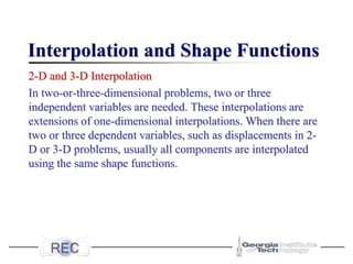
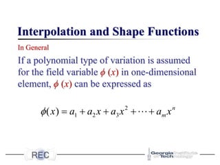
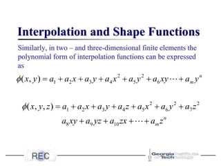
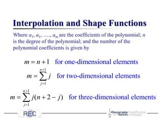
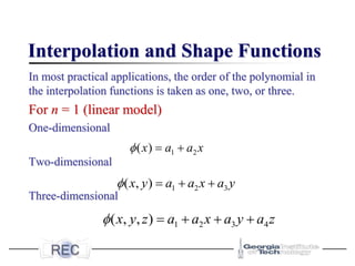
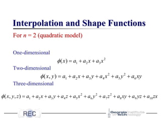
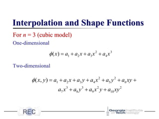
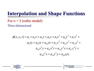
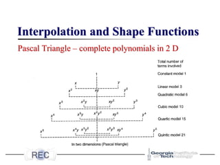
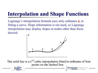
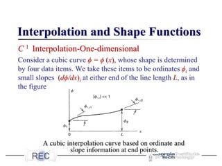
The document discusses interpolation and shape functions used in finite element analysis (FEA) to create continuous functions satisfying conditions at specified points, primarily utilizing polynomials. It describes how these functions can be structured in one, two, and three dimensions along with their continuity requirements and convergence conditions to ensure effective approximation of solutions. Additionally, it delves into linear and quadratic interpolation across different dimensions, detailing the formulation and characteristics of shape functions.

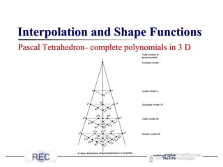
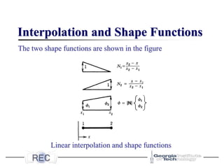
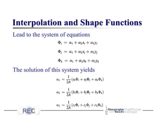
![Interpolation and Shape Functions
or
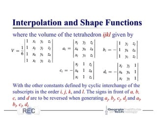
The ai can be expressed in terms of nodal values of
at known values of x. The relation between nodal
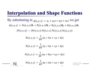
values of {ϕe }and ai is given as
}
]{
[ a
x
=
]
1
[
]
[ 2 n
x
x
x
x
=
1 2 3
{ } [ ]
T
m
a a a a a
=
}
]{
[
}
{ a
A
e =
](https://image.slidesharecdn.com/lecture5cee6504-interpolation-240903191227-69523928/85/FEM-Lecture-5-CEE6504-Interpolation-pdf-4-320.jpg)
![Interpolation and Shape Functions
2
1 1
1 1 1
2
2 2
2 2 2
2
3 3
3 3 3
2
1
1
{ } 1
1
n
n
n
e
n
m m
m m m
a
x x x
a
x x x
a
x x x
a
x x x
= =
}
]{
[
}
{ a
A
e =
](https://image.slidesharecdn.com/lecture5cee6504-interpolation-240903191227-69523928/85/FEM-Lecture-5-CEE6504-Interpolation-pdf-5-320.jpg)
![Interpolation and Shape Functions
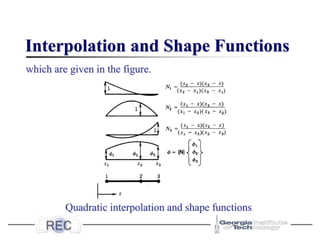
Recalling
}
{
]
[
}
{ 1
e
A
a
−
=
}
{
]
][
[ 1
e
A
x
−
=
}
]{
[ e
N
=
}
]{
[
}
{ a
A
e =
}
]{
[ a
x
=
](https://image.slidesharecdn.com/lecture5cee6504-interpolation-240903191227-69523928/85/FEM-Lecture-5-CEE6504-Interpolation-pdf-6-320.jpg)
![Interpolation and Shape Functions
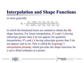
And
𝑁 = 𝑥 𝐴 −1 = 𝑁1 𝑁2 𝑁3 ⋯ 𝑁𝑚
An individual Ni in matrix [N] is called a shape
function. The name basis function sometimes used
instead.
}
]{
[ e
N
=](https://image.slidesharecdn.com/lecture5cee6504-interpolation-240903191227-69523928/85/FEM-Lecture-5-CEE6504-Interpolation-pdf-7-320.jpg)
![Interpolation and Shape Functions
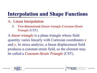
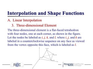
A. Linear Interpolation
1. One-dimensional
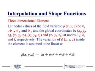
In FEA, with ϕ = u, the displacement field in the
linear case can be given as
or the displacement field can be given in the form
=
2
1
2
1 ]
[
N
N
=
2
1
2
1 ]
[
u
u
N
N
u](https://image.slidesharecdn.com/lecture5cee6504-interpolation-240903191227-69523928/85/FEM-Lecture-5-CEE6504-Interpolation-pdf-24-320.jpg)
![Interpolation and Shape Functions
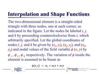
We begin with linear interpolation between points (x1, ϕ1) and
(x2, ϕ2) for which [x] = [1 x]. Evaluating at points 1 and 2,
we obtain
Inverting [A] and using we obtain
]
[
]
][
[
]
[ 2
1
1
N
N
A
x
N =
= −
1 1
2 2
a
A
a
=
](https://image.slidesharecdn.com/lecture5cee6504-interpolation-240903191227-69523928/85/FEM-Lecture-5-CEE6504-Interpolation-pdf-25-320.jpg)
![Interpolation and Shape Functions
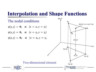
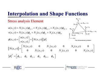
Stress analysis Element
The DOF’s at each node for this element are u and v. The
same linear interpolation is used for both dependent variables.
CST element for 2-D stress
analysis
=
3
2
1
]
1
[
a
a
a
y
x
u
=
6
5
4
]
1
[
a
a
a
y
x
v](https://image.slidesharecdn.com/lecture5cee6504-interpolation-240903191227-69523928/85/FEM-Lecture-5-CEE6504-Interpolation-pdf-33-320.jpg)
![Interpolation and Shape Functions
B. Quadratic Interpolation
1. One-dimensional. Quadratic interpolation fits a parabola to
the points (x1, ϕ1), (x2, ϕ2), and (x3, ϕ3). These points need not
be equidistant. Matrix [x] = [1 x x2] and
This equation yields the shape
functions
]
[
]
][
[
]
[ 3
2
1
1
N
N
N
A
x
N =
= −
1 1
2 2
3 3
a
A a
a
=
](https://image.slidesharecdn.com/lecture5cee6504-interpolation-240903191227-69523928/85/FEM-Lecture-5-CEE6504-Interpolation-pdf-41-320.jpg)
![Interpolation and Shape Functions
The foregoing shape functions have the following
characteristics:
◼ All shape functions Ni , along with function ϕ itself, are
polynomial of the same degree.
◼ For any shape function Ni , Ni = 1 when x = xi and Ni = 0
when x = xj for any integer j ≠ i. That is Ni is unity at its own
node but is zero at other nodes.
◼ C 0 shape functions sum to unity; that is, ∑ Ni = 1. This
conclusion is implied by ϕ = [N]{ϕe}, because we must obtain
ϕ = 1when {ϕe} is a column of 1’s.](https://image.slidesharecdn.com/lecture5cee6504-interpolation-240903191227-69523928/85/FEM-Lecture-5-CEE6504-Interpolation-pdf-44-320.jpg)
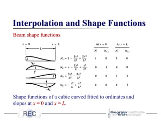
![Interpolation and Shape Functions
Now [x] = [1 x x2 x3], and upon evaluating ϕ and ϕ ,x at x
= 0 and x = L, the equation {ϕ e} = [A]{a} becomes
The obtained shape function are nothing but the four lateral
displacements and rotations of beam nodes.
1 1
, 1 2
2 3
, 2 4
x
x
a
a
A
a
a
=
](https://image.slidesharecdn.com/lecture5cee6504-interpolation-240903191227-69523928/85/FEM-Lecture-5-CEE6504-Interpolation-pdf-47-320.jpg)