Download as PDF, PPTX
![Results
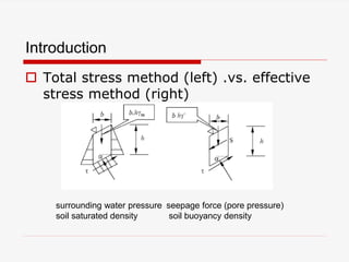
Comparison of different methods
FE Limited Equilibrium
KS KF KB
Case 1 Surface 1 [13.4 , 9.2 , 9.2 ] 1.190 1.095 1.069
surface 2 [13.4 , 8.0 , 8.0 ] 1.216 1.088 1.155
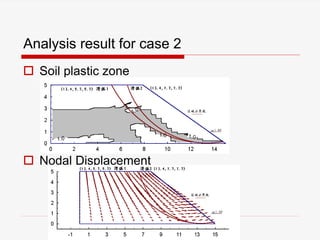
Case 2 Surface 1 [13.4 , 9.2 , 9.2 ] 1.125 1.070 1.031
surface 2 [13.4 , 8.0 , 8.0 ] 1.172 1.075 1.057
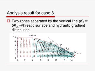
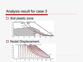
Case 3 Surface 1 [13.4 , 9.2 , 9.2 ] 1.078 1.119 1.067
surface 2 [13.4 , 8.0 , 8.0 ] 1.215 1.100 1.067
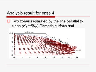
Case 4 Surface 1 [13.4 , 9.2 , 9.2 ] 1.075 1.030 0.994
surface 2 [13.4 , 8.0 , 8.0 ] 1.077 1.018 1.067](https://image.slidesharecdn.com/fecodinganalysisonseepageandslopestability-200213013837/85/FE-coding-and-Analysis-on-Seepage-and-slope-stability-26-320.jpg)
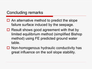


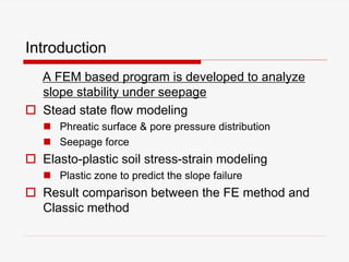
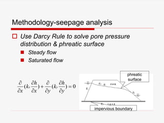
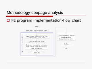
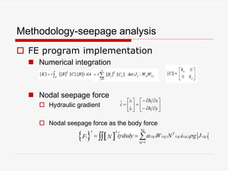
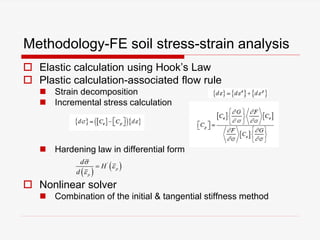
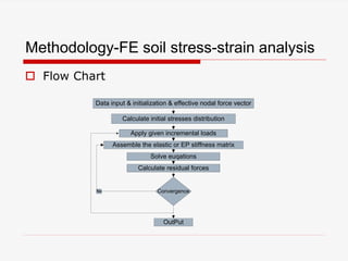
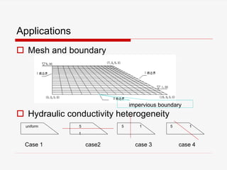
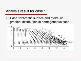
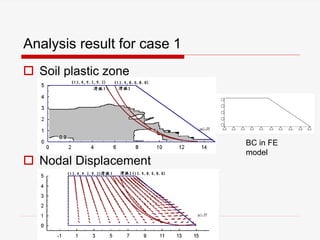
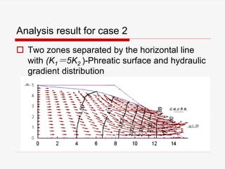
The document presents a finite element analysis (FEA) of groundwater seepage and soil slope stability, detailing methodologies for modeling seepage effects on soil stability. It discusses the implementation of a FEA program for analyzing pore pressure distribution, phreatic surface, and elasto-plastic soil stress-strain responses under varying conditions. The results indicate that non-homogeneous hydraulic conductivity significantly impacts soil slope stability, with findings closely aligning with traditional limit equilibrium methods.