Chapter 7
Externalities
Reading
• Essential reading
– Hindriks, J and G.D. Myles Intermediate Public Economics.
(Cambridge: MIT Press, 2006) Chapter 7.
• Further reading
– Bator, F.M. (1958) ‘The anatomy of market failure’, Quarterly
Journal of Economics, 72, 351—378.
– Buchanan, J.M. and C. Stubblebine (1962) ‘Externality’,
Economica, 29, 371—384.
– Coase, R.H. (1960) ‘The problem of social cost’, Journal of Law
and Economics, 3, 1—44.
– Lin, S. (ed.) Theory and Measurement of Economic Externalities.
(New York: Academic Press, 1976) [ISBN 0124504507 hbk].
– Meade, J.E. (1952) ‘External economies and diseconomies in a
competitive situation’, Economic Journal, 62, 54—76.
Reading
– Pigou, A.C. The Economics of Welfare. (London:
Macmillan, 1918).
• Challenging reading
– Muthoo, A. Bargaining Theory with Applications.
(Cambridge: Cambridge University Press, 1999)
[ISBN 0521576474 pbk].
– Starrett, D. (1972) ‘Fundamental non-convexities in
the theory of externalities’, Journal of Economic
Theory, 4, 180—199.
– Weitzman, M.L. (1974) ‘Prices vs. quantities’, Review
of Economic Studies, 41, 477—491.
Introduction
• An externality is a link between economic agents
that lies outside the price system
– Pollution from a factory
– Envy of a neighbor
• Externalities are not under the control of the
affected agent
– Efficiency theorems do not apply
– Competitive equilibrium unlikely to be efficient
• Externalities are of practical importance
– Global warming
– Damage to ozone layer
Externalities Defined
• An externality is present whenever some
economic agent’s welfare is “directly” affected
the action of another agent in the economy
• Production externality: the externality affects
profit
• Consumption externality: the externality affects
utility
• Positive externality: raises utility or profit
• Negative externality: reduces utility or profit
Externalities Defined
• Pecuniary externality: an external effect that
works through prices
– An oil price rise affects the profitability of a fishery
• Pecuniary externalities do not create an
inefficiency
• With externalities the actions of agents are not
independent and not determined solely by prices
– Strategic interdependence arises
– This is the source of inefficiency
Market Inefficiency
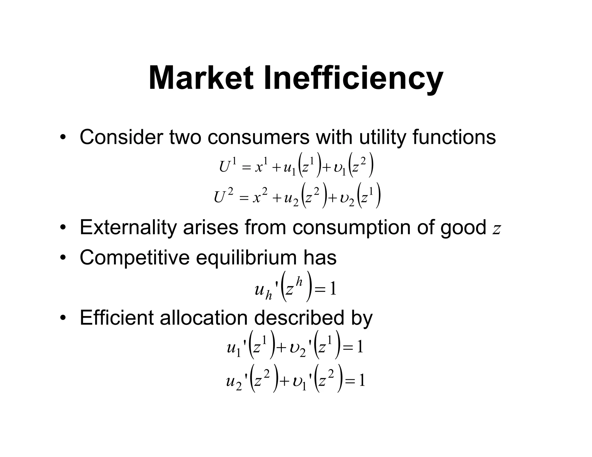
• Consider two consumers with utility functions
• Externality arises from consumption of good z
• Competitive equilibrium has
• Efficient allocation described by
   
2
1
1
1
1
1
z
z
u
x
U 



   
1
2
2
2
2
2
z
z
u
x
U 



  1
' 
h
h z
u
    1
'
' 1
2
1
1 
 z
z
u 
    1
'
' 2
1
2
2 
 z
z
u 
Market Inefficiency
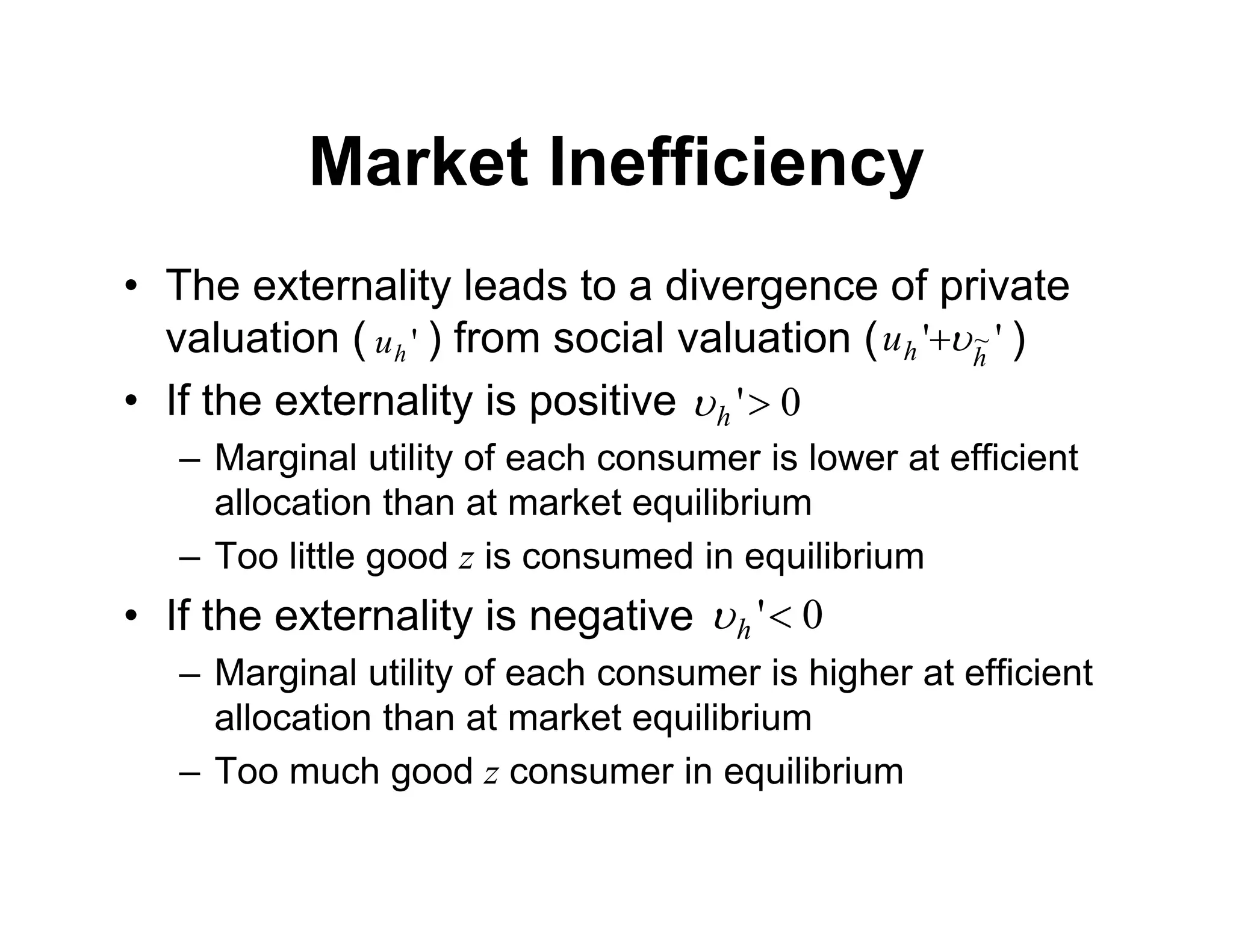
• The externality leads to a divergence of private
valuation ( ) from social valuation ( )
• If the externality is positive
– Marginal utility of each consumer is lower at efficient
allocation than at market equilibrium
– Too little good z is consumed in equilibrium
• If the externality is negative
– Marginal utility of each consumer is higher at efficient
allocation than at market equilibrium
– Too much good z consumer in equilibrium
0
'
h

0
'
h

'
h
u '
' ~
h
h
u 

Market Inefficiency
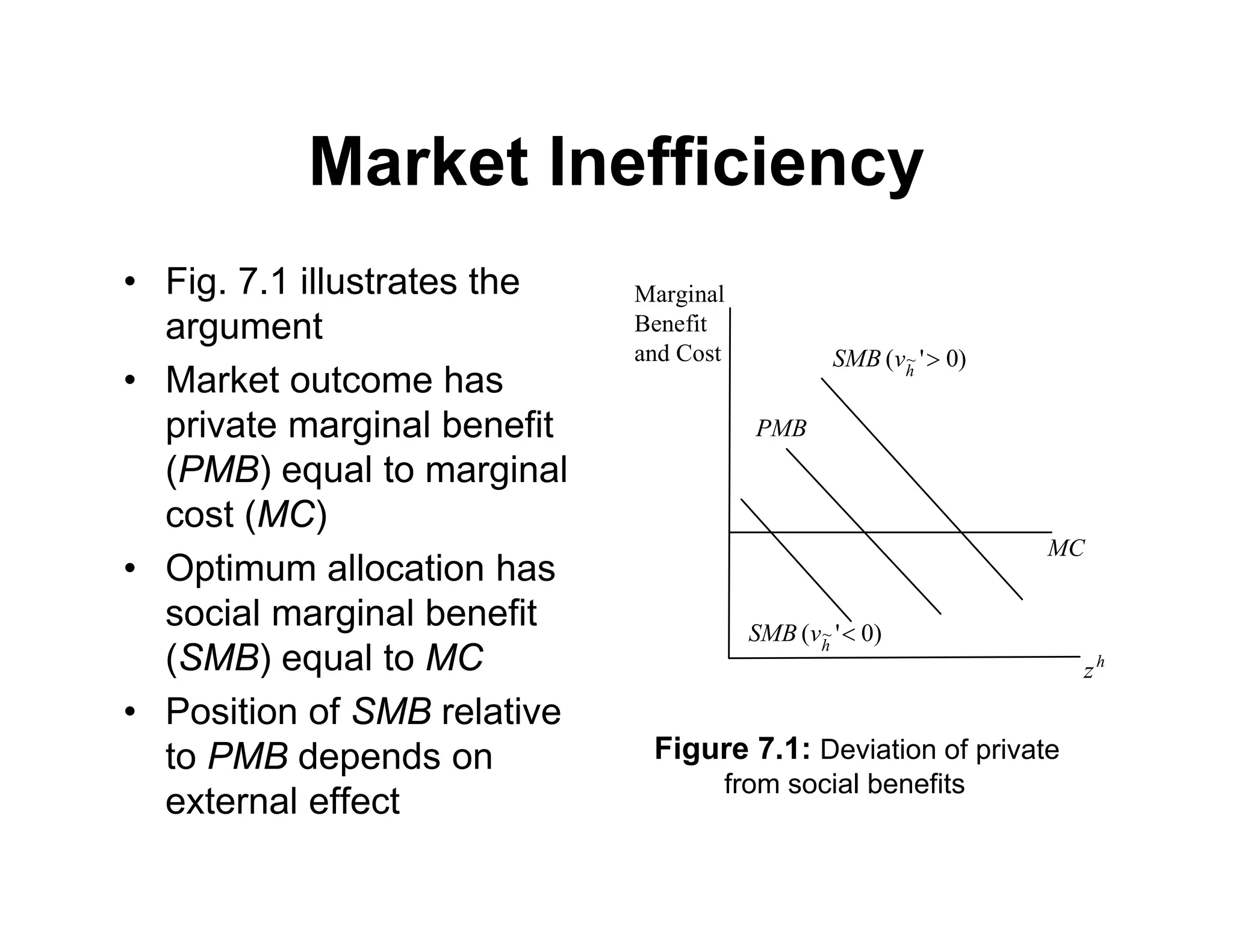
• Fig. 7.1 illustrates the
argument
• Market outcome has
private marginal benefit
(PMB) equal to marginal
cost (MC)
• Optimum allocation has
social marginal benefit
(SMB) equal to MC
• Position of SMB relative
to PMB depends on
external effect
PMB
MC
h
z
Marginal
Benefit
and Cost )
0
'
( ~ 
h
v
SMB
)
0
'
( ~ 
h
v
SMB
Figure 7.1: Deviation of private
from social benefits
Externality Examples
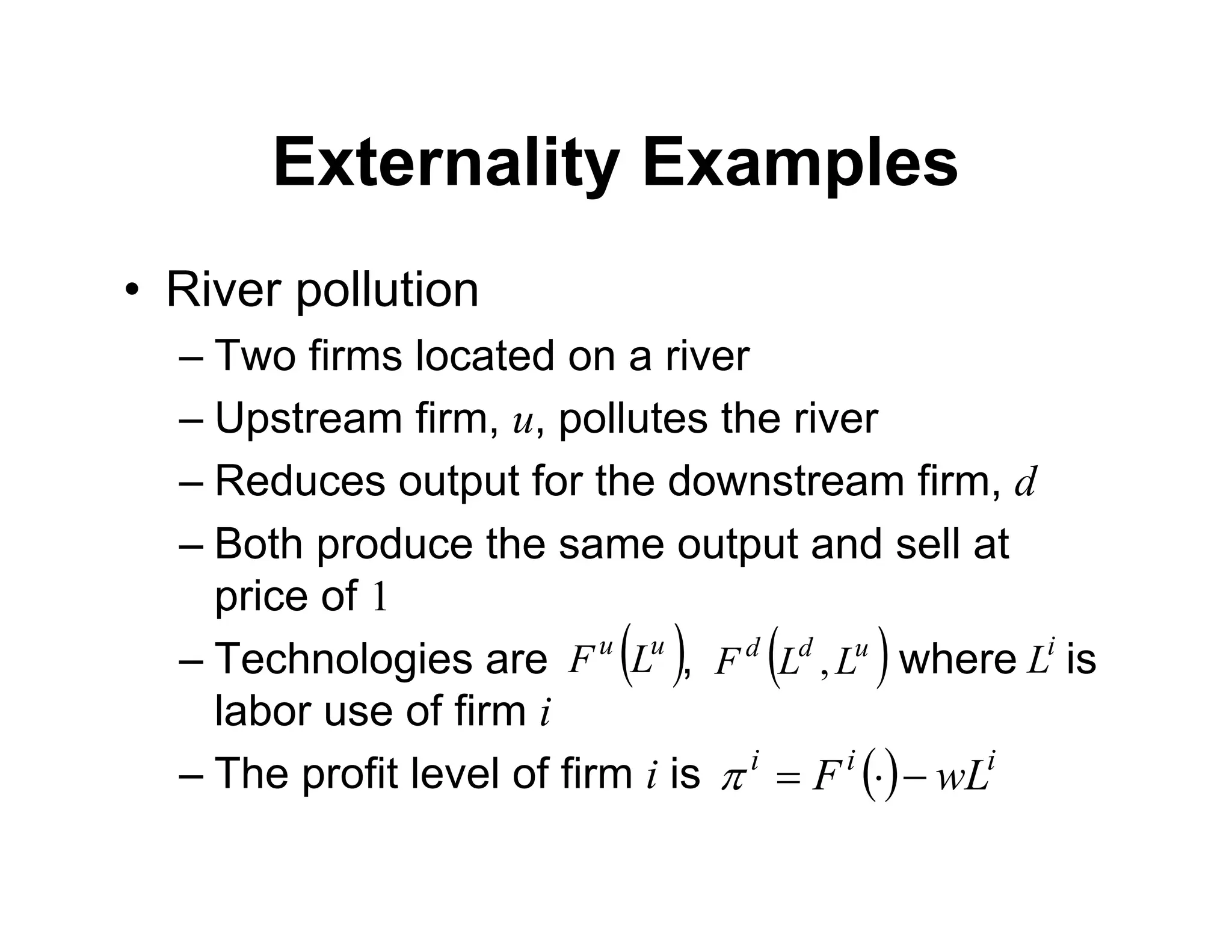
• River pollution
– Two firms located on a river
– Upstream firm, u, pollutes the river
– Reduces output for the downstream firm, d
– Both produce the same output and sell at
price of 1
– Technologies are , where is
labor use of firm i
– The profit level of firm i is
 
u
u
L
F  
u
d
d
L
L
F ,
 i
i
i
wL
F 



i
L
w
0u 0d
w
Upstream
Downstream
Revenue
Revenue
Cost
Cost
u

*
*
, d
u
L
L
d

Externality Examples
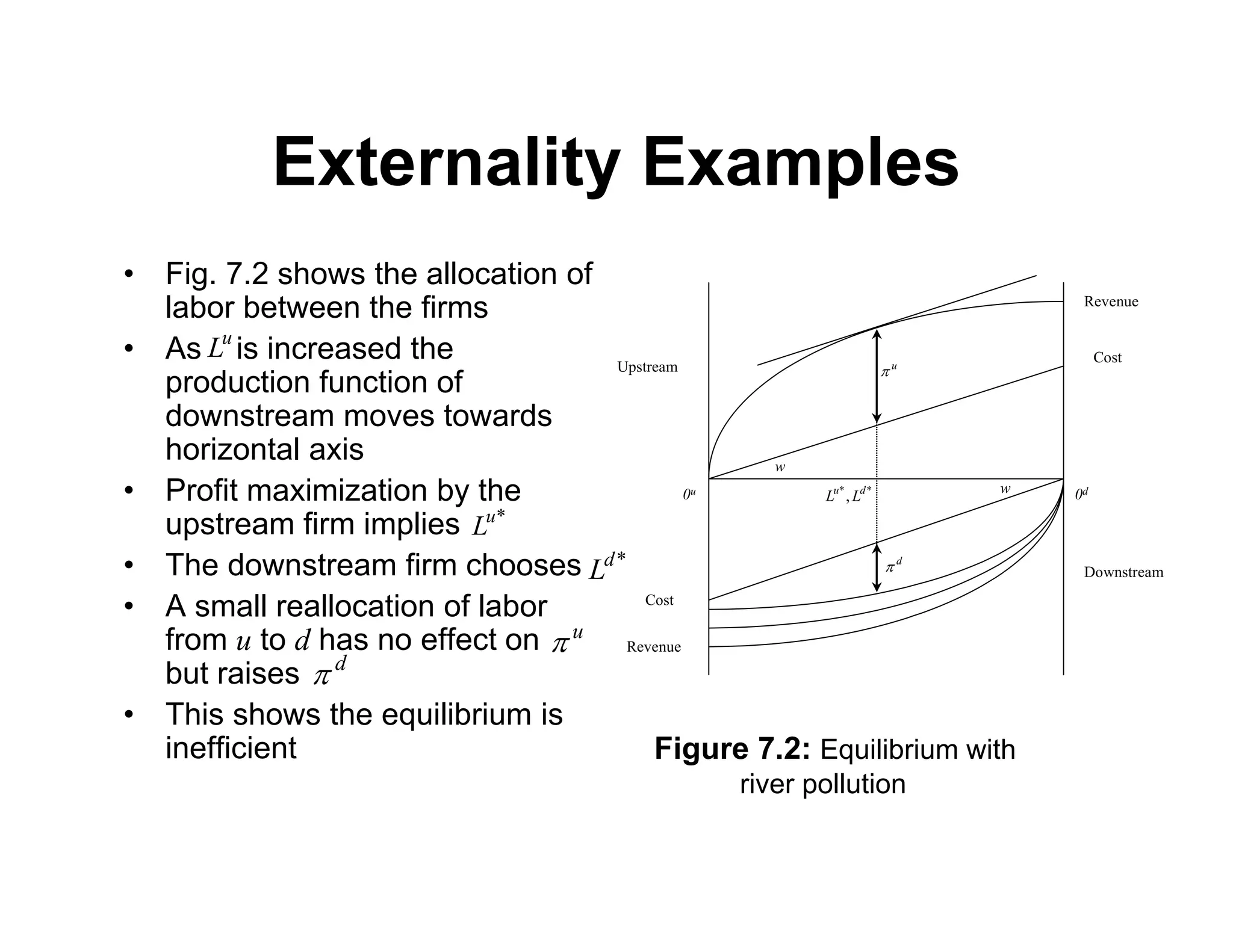
• Fig. 7.2 shows the allocation of
labor between the firms
• As is increased the
production function of
downstream moves towards
horizontal axis
• Profit maximization by the
upstream firm implies
• The downstream firm chooses
• A small reallocation of labor
from u to d has no effect on
but raises
• This shows the equilibrium is
inefficient
*
u
L
Figure 7.2: Equilibrium with
river pollution
*
d
L
u
L
u

d

Externality Examples
• Traffic Jams
– This example shows the externalities that car
drivers impose on each other
– Assume there are N commuters with a choice
of train or car
– Travel by train takes 40 minutes
– The travel time by car increases as the
number of car users increases
– Commuters make the choice which minimizes
their personal travel time
Externality Examples
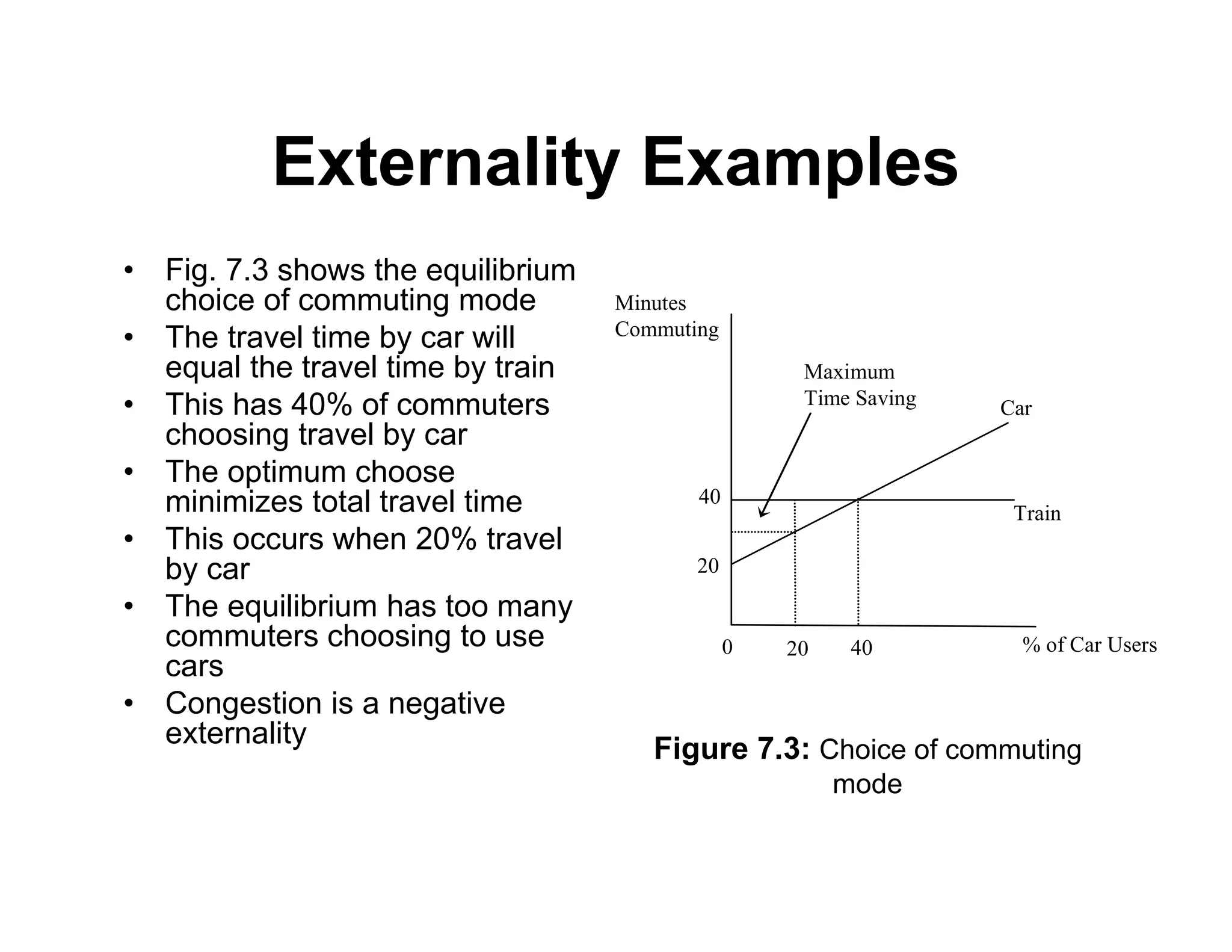
• Fig. 7.3 shows the equilibrium
choice of commuting mode
• The travel time by car will
equal the travel time by train
• This has 40% of commuters
choosing travel by car
• The optimum choose
minimizes total travel time
• This occurs when 20% travel
by car
• The equilibrium has too many
commuters choosing to use
cars
• Congestion is a negative
externality
Minutes
Commuting
Train
Maximum
Time Saving
0
Car
20 40
20
40
% of Car Users
Figure 7.3: Choice of commuting
mode
Externality Examples
• Pecuniary Externality
– A group of students must choose to be
economists or lawyers
– Income declines when more students make
the same choice
– This is a pecuniary externality since an
additional student choosing to be an
economist lowers income for all economists
– Each individual ignores this externality when
choosing occupation
Externality Examples
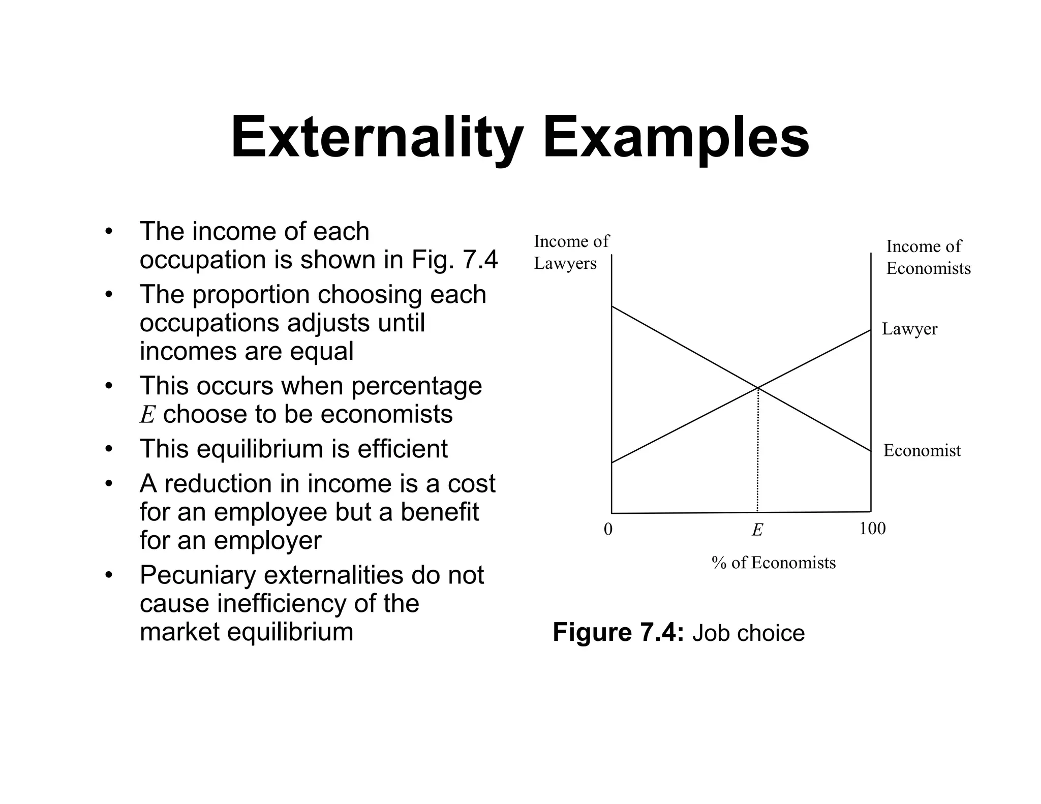
• The income of each
occupation is shown in Fig. 7.4
• The proportion choosing each
occupations adjusts until
incomes are equal
• This occurs when percentage
E choose to be economists
• This equilibrium is efficient
• A reduction in income is a cost
for an employee but a benefit
for an employer
• Pecuniary externalities do not
cause inefficiency of the
market equilibrium
Income of
Lawyers
Economist
0
Lawyer
100
% of Economists
Income of
Economists
E
Figure 7.4: Job choice
Externality Examples
• The Rat Race Problem
– The rat race is a contest for relative position
– Assume performance is judged in relative
terms and not absolute terms
– An advantage is gained over rivals only by
competing harder than they do
– If all competitors compete hard the extra
efforts cancels out
– All competitors could gain by making an
agreement to reduce effort
Externality Examples
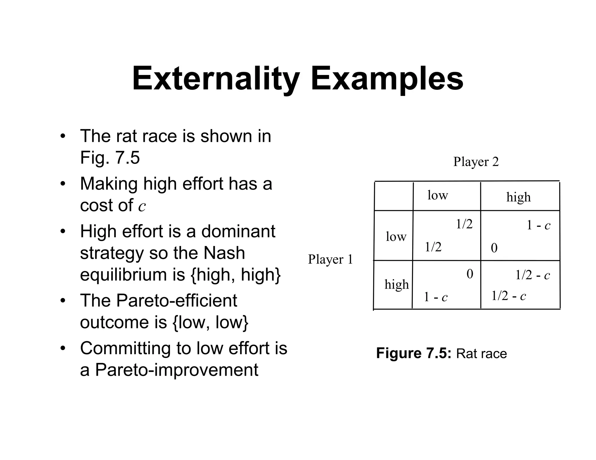
• The rat race is shown in
Fig. 7.5
• Making high effort has a
cost of c
• High effort is a dominant
strategy so the Nash
equilibrium is {high, high}
• The Pareto-efficient
outcome is {low, low}
• Committing to low effort is
a Pareto-improvement
Player 2
Player 1
low
low
high
1/2
1/2
0
1 - c
1/2 - c
0
high
1 - c
1/2 - c
Figure 7.5: Rat race
Externality Examples
• The Tragedy of the Commons
– This example arises from the common right of
access to a resource
– Consider a lake that is used by local
fisherman who can earn wage w if they do not
fish
– The fishermen rent boats on a daily basis at
cost c
– If B boats are hired each fisherman catches
F(B) fish
Externality Examples
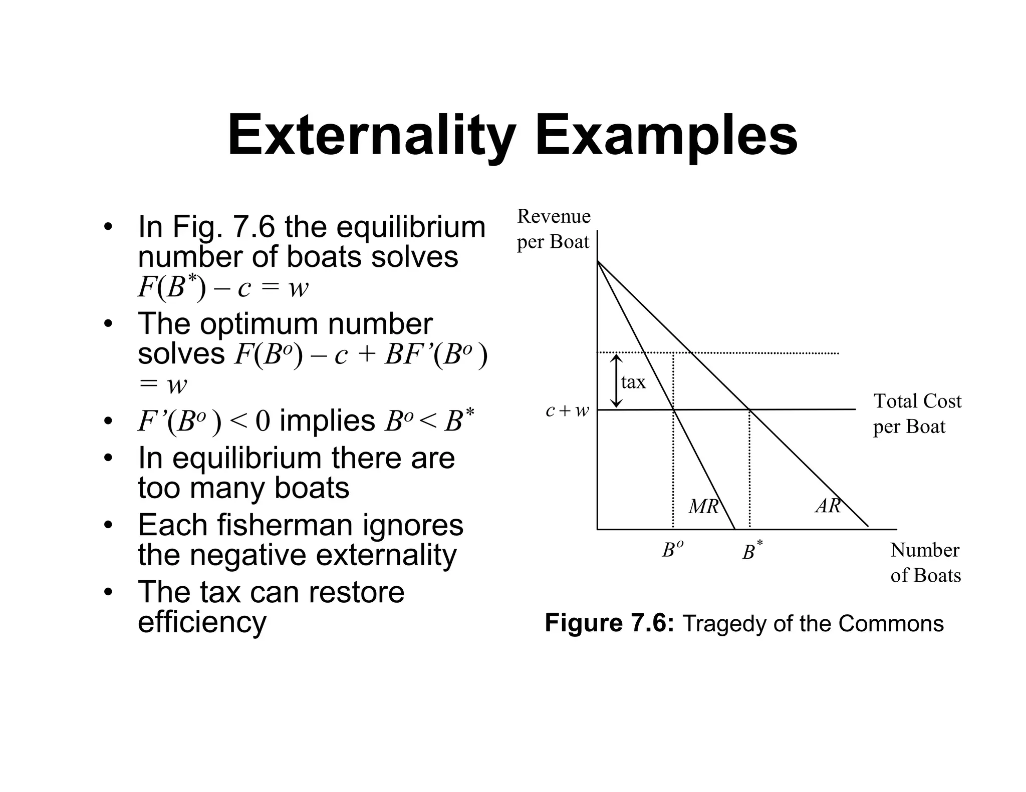
• In Fig. 7.6 the equilibrium
number of boats solves
F(B*) – c = w
• The optimum number
solves F(Bo) – c + BF’(Bo )
= w
• F’(Bo ) < 0 implies Bo < B*
• In equilibrium there are
too many boats
• Each fisherman ignores
the negative externality
• The tax can restore
efficiency
w
c 
tax
Total Cost
per Boat
Revenue
per Boat
Number
of Boats
*
B
o
B
AR
MR
Figure 7.6: Tragedy of the Commons
Externality Examples
• Bandwagon Effect
– The bandwagon effect studies how standards
are adopted and wrong standards may be
sustained
– The standard example is the typewriter
keyboard
– The Qwerty keyboard was designed to
prevent jamming of mechanical keys
– It is claimed that faster keyboards can be
designed
– Typists are reluctant to switch given their skills
Externality Examples
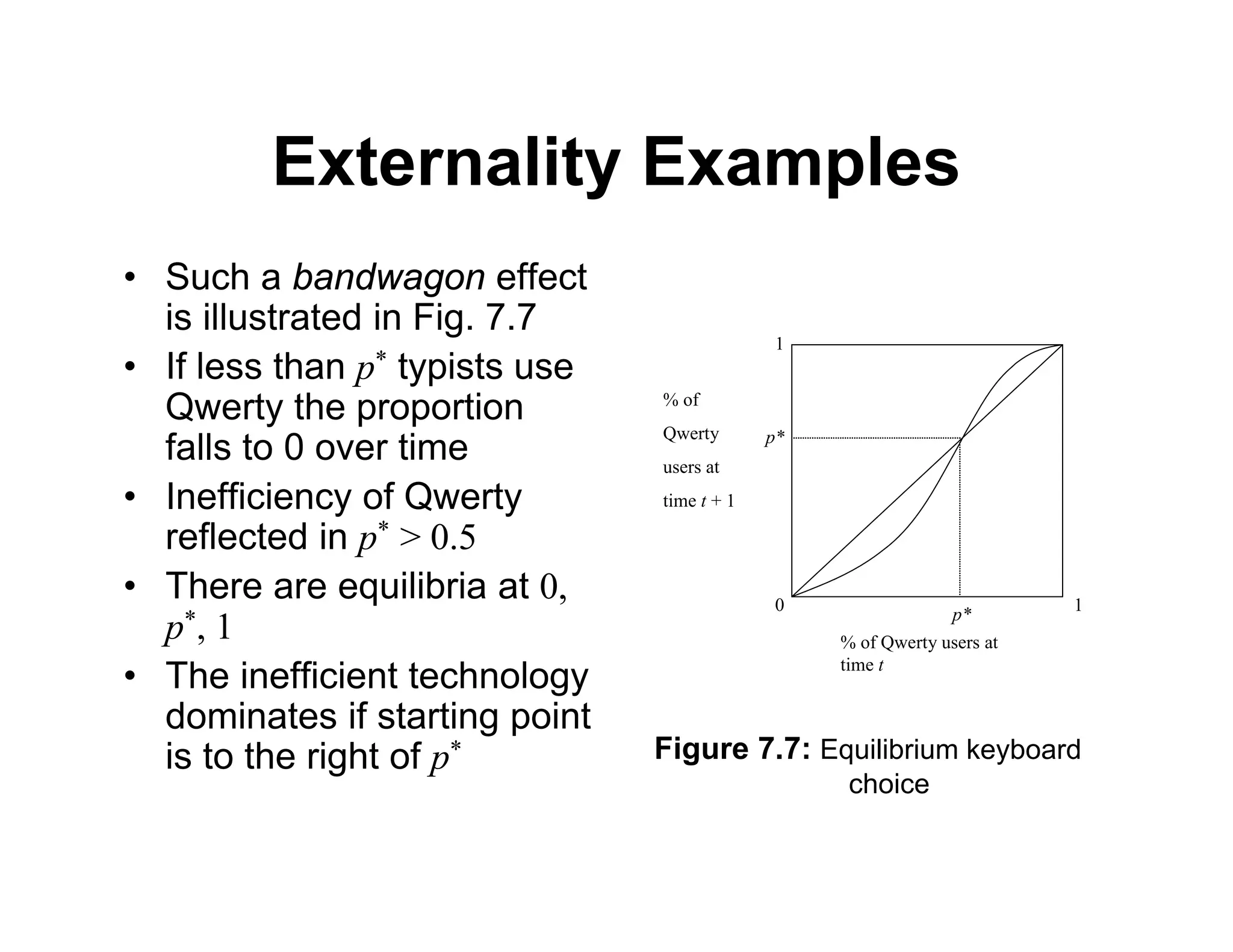
• Such a bandwagon effect
is illustrated in Fig. 7.7
• If less than p* typists use
Qwerty the proportion
falls to 0 over time
• Inefficiency of Qwerty
reflected in p* > 0.5
• There are equilibria at 0,
p*, 1
• The inefficient technology
dominates if starting point
is to the right of p* Figure 7.7: Equilibrium keyboard
choice
0
1
1
p*
p*
% of Qwerty users at
time t
% of
Qwerty
users at
time t + 1
Pigouvian Taxation
• Externalities cause inefficiency because of the
divergence between social and private benefits
(or costs)
• A tax can be used to raise the private marginal
cost
– This assists efficiency with a negative externality
• A subsidy can be used to reduce the private
marginal cost
– This assists efficiency with a positive externality
• Taxes used to combat externalities are called
Pigouvian taxes
Pigouvian Taxation
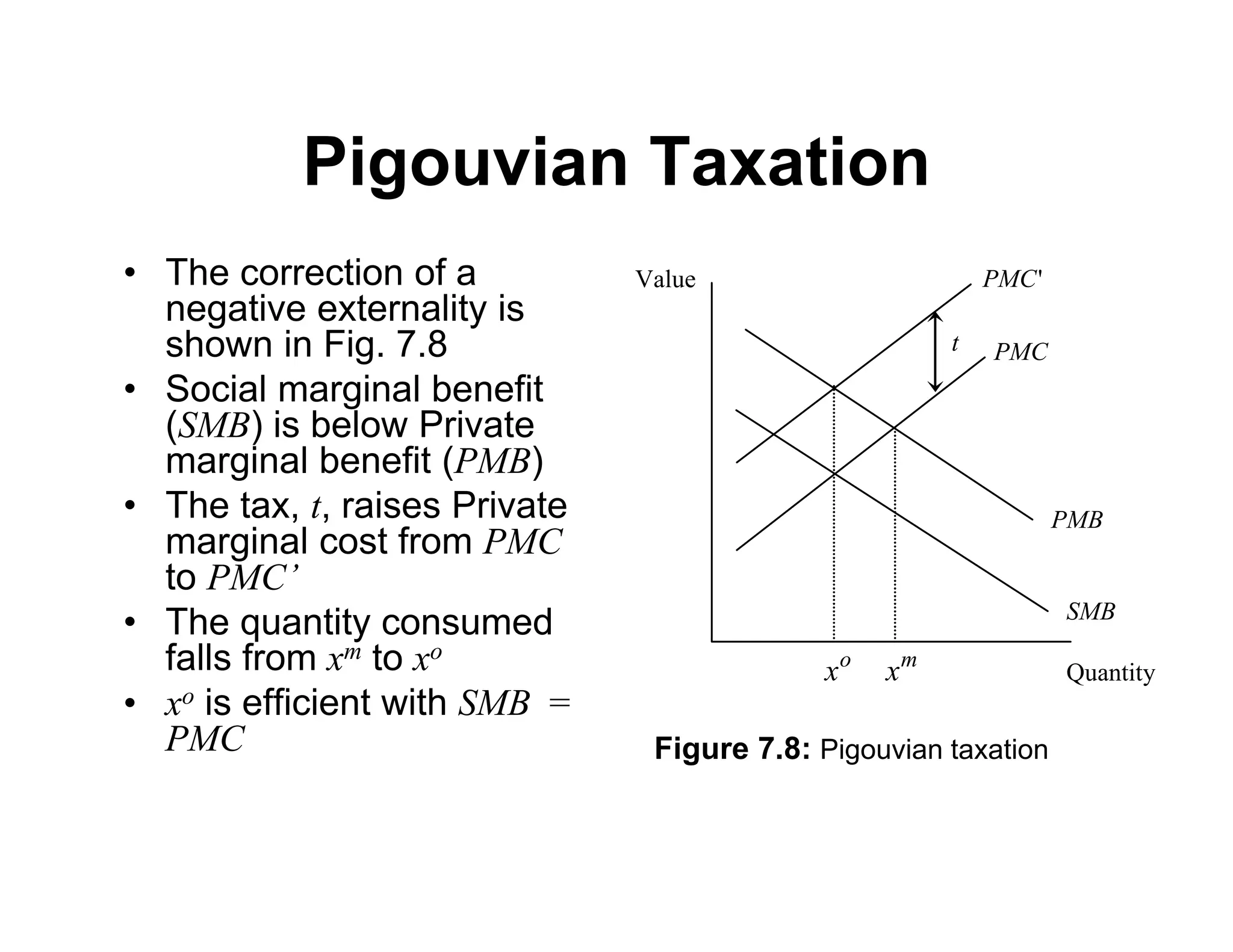
• The correction of a
negative externality is
shown in Fig. 7.8
• Social marginal benefit
(SMB) is below Private
marginal benefit (PMB)
• The tax, t, raises Private
marginal cost from PMC
to PMC’
• The quantity consumed
falls from xm to xo
• xo is efficient with SMB =
PMC
Quantity
Value
PMB
SMB
PMC
o
x m
x
t
'
PMC
Figure 7.8: Pigouvian taxation
Pigouvian Taxation
• Pigouvian taxation appears a simple solution
– A tax is paid equal to the marginal damage
– A subsidy is received equal to marginal benefit
• There are limitations to the argument
– Taxes may need to be differentiated between
consumers, firms, and goods
– Without sufficient differentiation the externality is only
partially corrected
– Intervention may also be required markets for related
goods
• Taxation should be seen as putting a price on
the externality
Licenses
• Licenses can control externalities directly
– Legislate that externalities can only be generated if a
license is held
• The optimal quantity of externality is calculated
• Licenses totalling to this quantity are issued
• Trading of licenses ensures they are used by
those who obtain the greatest benefit
• Administratively this is simpler than taxation
• But licenses have no information advantage
Licenses
• Licenses and taxes have
different outcome with
uncertainty
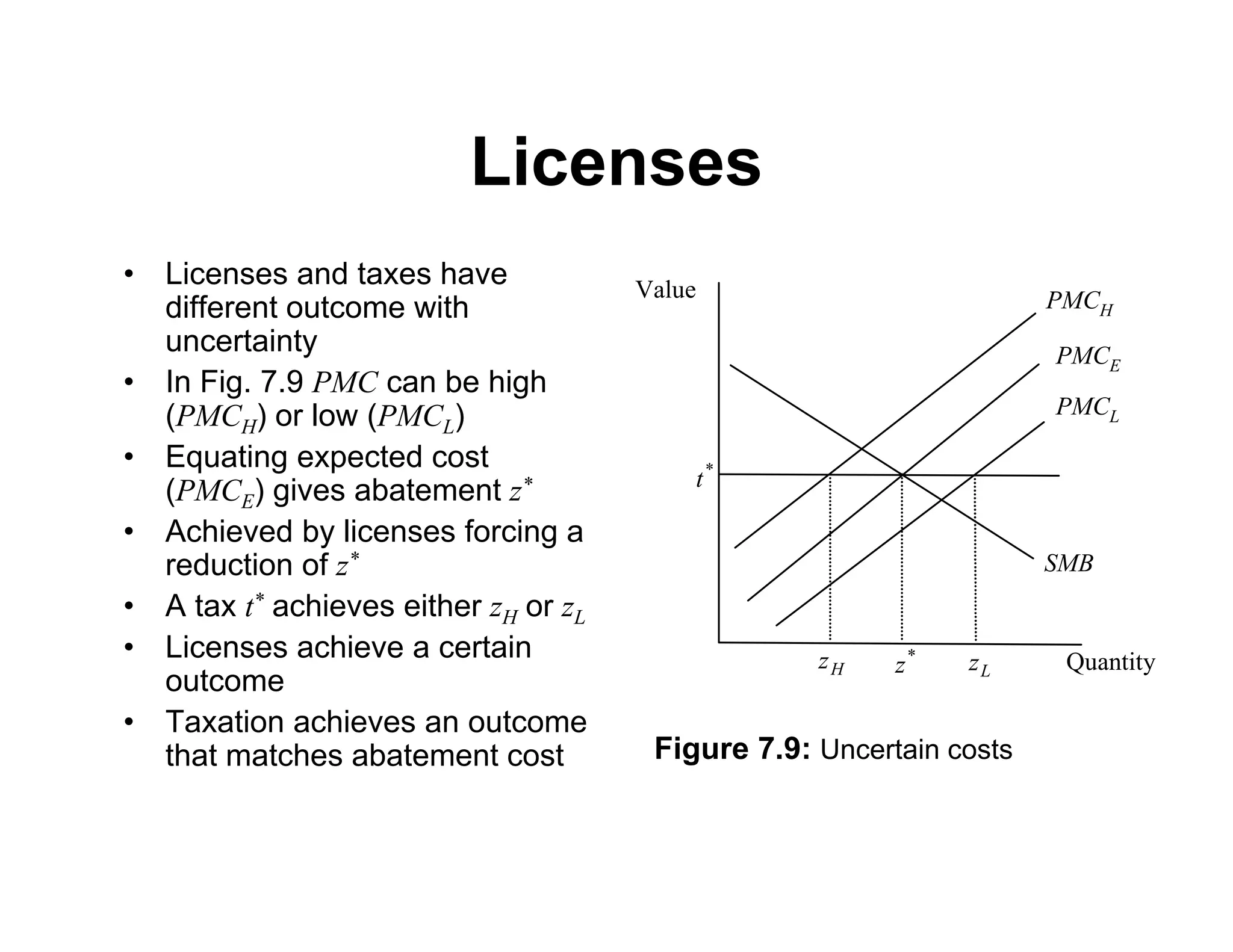
• In Fig. 7.9 PMC can be high
(PMCH) or low (PMCL)
• Equating expected cost
(PMCE) gives abatement z*
• Achieved by licenses forcing a
reduction of z*
• A tax t* achieves either zH or zL
• Licenses achieve a certain
outcome
• Taxation achieves an outcome
that matches abatement cost
Quantity
Value
SMB
PMCE
PMCH
PMCL
*
z L
z
H
z
*
t
Figure 7.9: Uncertain costs
Internalization
• Consider two producers who each causes a
positive externality for the other
– A beekeeper and an orchard
• With no intervention each will ignore externality
and produce too little
• If combined into a single firm they will internalize
the externality and produce at the efficient level
• But this may cause monopoly
• It may require unwilling partners to cooperate
The Coase Theorem
• The Coase Theorem proposes that economic
agents will solve externality problems without
intervention
• The theorem can be stated as follows:
“In a competitive economy with complete information
and zero transaction costs, the allocation of resources
will be efficient and invariant with respect to legal
rules of entitlement.”
• Legal rules of entitlement (or property rights)
determine ownership in the economy
The Coase Theorem
• Coase sees externalities as arising through the
absence of property rights
– Pollution occurs when there is no right to clean air or
clean water
• If there was a property right anyone suffering an
externality would be paid compensation
• The compensation is a price for the externality
• Competitive trading will ensure the correct price
emerges and efficiency is achieved
The Coase Theorem
• The theorem also asserts that the equilibrium is
invariant to assignment of property rights
• Will a firm pollute the atmosphere of a
neighboring house?
– Only if the benefit from doing so exceeds the
compensation required by the householder
– This applies whether the firm has the right to pollute
or the householder has the right to clean air
• The final distribution of income will be different
• Equilibrium will be unaffected by the allocation of
property rights if there are no income effects
The Coase Theorem
• The practical limitations of the Coase theorem
are:
– The lack of clear property rights
– Transaction costs in reaching compensation
agreements
– The potential thinness of the market implying bilateral
bargaining and potential inefficiency with incomplete
information
– Potential monopoly power
• The Coase theorem suggests a resolution to the
externality problem but there are reasons why
the market may not function
Nonconvexity
• Convexity ensures economic optimizations have
well defined solutions
– Convexity of preferences implies mixtures preferred
– Convexity of technology prevents increasing returns
• Externalities are a source of nonconvexity
through their effect on technology
• An economy with nonconvexity may not have an
equilibrium
• Even if it has an equilibrium it may not be
possible for pricing to achieve the efficient
equilibrium
Nonconvexity
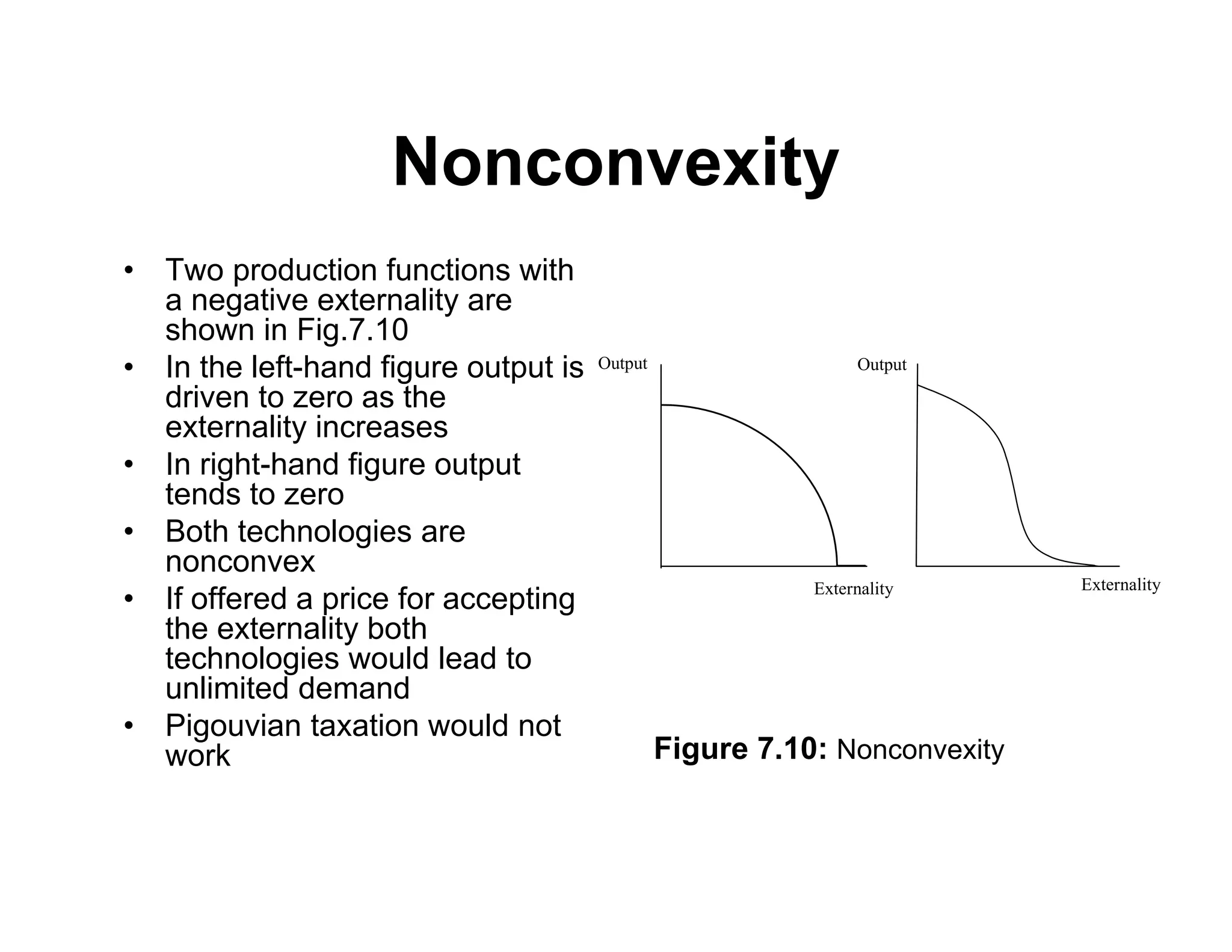
• Two production functions with
a negative externality are
shown in Fig.7.10
• In the left-hand figure output is
driven to zero as the
externality increases
• In right-hand figure output
tends to zero
• Both technologies are
nonconvex
• If offered a price for accepting
the externality both
technologies would lead to
unlimited demand
• Pigouvian taxation would not
work
Externality Externality
Output Output
Figure 7.10: Nonconvexity
Conclusions
• Externalities are a feature of economic activity
• The existence of externalities can lead to
inefficiency when the conditions of the Coase
theorem do not apply
• Pigouvian taxes can reduce the inefficiency but
require excessive differentiation
• Marketable licenses can also help and have
simpler administration
• But all solutions require the same information for
implementation

externalities_hindriks_myles_ch7_slides.pdf

  • 1.
  • 2.
    Reading • Essential reading –Hindriks, J and G.D. Myles Intermediate Public Economics. (Cambridge: MIT Press, 2006) Chapter 7. • Further reading – Bator, F.M. (1958) ‘The anatomy of market failure’, Quarterly Journal of Economics, 72, 351—378. – Buchanan, J.M. and C. Stubblebine (1962) ‘Externality’, Economica, 29, 371—384. – Coase, R.H. (1960) ‘The problem of social cost’, Journal of Law and Economics, 3, 1—44. – Lin, S. (ed.) Theory and Measurement of Economic Externalities. (New York: Academic Press, 1976) [ISBN 0124504507 hbk]. – Meade, J.E. (1952) ‘External economies and diseconomies in a competitive situation’, Economic Journal, 62, 54—76.
  • 3.
    Reading – Pigou, A.C.The Economics of Welfare. (London: Macmillan, 1918). • Challenging reading – Muthoo, A. Bargaining Theory with Applications. (Cambridge: Cambridge University Press, 1999) [ISBN 0521576474 pbk]. – Starrett, D. (1972) ‘Fundamental non-convexities in the theory of externalities’, Journal of Economic Theory, 4, 180—199. – Weitzman, M.L. (1974) ‘Prices vs. quantities’, Review of Economic Studies, 41, 477—491.
  • 4.
    Introduction • An externalityis a link between economic agents that lies outside the price system – Pollution from a factory – Envy of a neighbor • Externalities are not under the control of the affected agent – Efficiency theorems do not apply – Competitive equilibrium unlikely to be efficient • Externalities are of practical importance – Global warming – Damage to ozone layer
  • 5.
    Externalities Defined • Anexternality is present whenever some economic agent’s welfare is “directly” affected the action of another agent in the economy • Production externality: the externality affects profit • Consumption externality: the externality affects utility • Positive externality: raises utility or profit • Negative externality: reduces utility or profit
  • 6.
    Externalities Defined • Pecuniaryexternality: an external effect that works through prices – An oil price rise affects the profitability of a fishery • Pecuniary externalities do not create an inefficiency • With externalities the actions of agents are not independent and not determined solely by prices – Strategic interdependence arises – This is the source of inefficiency
  • 7.
    Market Inefficiency • Considertwo consumers with utility functions • Externality arises from consumption of good z • Competitive equilibrium has • Efficient allocation described by     2 1 1 1 1 1 z z u x U         1 2 2 2 2 2 z z u x U       1 '  h h z u     1 ' ' 1 2 1 1   z z u      1 ' ' 2 1 2 2   z z u 
  • 8.
    Market Inefficiency • Theexternality leads to a divergence of private valuation ( ) from social valuation ( ) • If the externality is positive – Marginal utility of each consumer is lower at efficient allocation than at market equilibrium – Too little good z is consumed in equilibrium • If the externality is negative – Marginal utility of each consumer is higher at efficient allocation than at market equilibrium – Too much good z consumer in equilibrium 0 ' h  0 ' h  ' h u ' ' ~ h h u  
  • 9.
    Market Inefficiency • Fig.7.1 illustrates the argument • Market outcome has private marginal benefit (PMB) equal to marginal cost (MC) • Optimum allocation has social marginal benefit (SMB) equal to MC • Position of SMB relative to PMB depends on external effect PMB MC h z Marginal Benefit and Cost ) 0 ' ( ~  h v SMB ) 0 ' ( ~  h v SMB Figure 7.1: Deviation of private from social benefits
  • 10.
    Externality Examples • Riverpollution – Two firms located on a river – Upstream firm, u, pollutes the river – Reduces output for the downstream firm, d – Both produce the same output and sell at price of 1 – Technologies are , where is labor use of firm i – The profit level of firm i is   u u L F   u d d L L F ,  i i i wL F     i L
  • 11.
    w 0u 0d w Upstream Downstream Revenue Revenue Cost Cost u  * * , d u L L d  ExternalityExamples • Fig. 7.2 shows the allocation of labor between the firms • As is increased the production function of downstream moves towards horizontal axis • Profit maximization by the upstream firm implies • The downstream firm chooses • A small reallocation of labor from u to d has no effect on but raises • This shows the equilibrium is inefficient * u L Figure 7.2: Equilibrium with river pollution * d L u L u  d 
  • 12.
    Externality Examples • TrafficJams – This example shows the externalities that car drivers impose on each other – Assume there are N commuters with a choice of train or car – Travel by train takes 40 minutes – The travel time by car increases as the number of car users increases – Commuters make the choice which minimizes their personal travel time
  • 13.
    Externality Examples • Fig.7.3 shows the equilibrium choice of commuting mode • The travel time by car will equal the travel time by train • This has 40% of commuters choosing travel by car • The optimum choose minimizes total travel time • This occurs when 20% travel by car • The equilibrium has too many commuters choosing to use cars • Congestion is a negative externality Minutes Commuting Train Maximum Time Saving 0 Car 20 40 20 40 % of Car Users Figure 7.3: Choice of commuting mode
  • 14.
    Externality Examples • PecuniaryExternality – A group of students must choose to be economists or lawyers – Income declines when more students make the same choice – This is a pecuniary externality since an additional student choosing to be an economist lowers income for all economists – Each individual ignores this externality when choosing occupation
  • 15.
    Externality Examples • Theincome of each occupation is shown in Fig. 7.4 • The proportion choosing each occupations adjusts until incomes are equal • This occurs when percentage E choose to be economists • This equilibrium is efficient • A reduction in income is a cost for an employee but a benefit for an employer • Pecuniary externalities do not cause inefficiency of the market equilibrium Income of Lawyers Economist 0 Lawyer 100 % of Economists Income of Economists E Figure 7.4: Job choice
  • 16.
    Externality Examples • TheRat Race Problem – The rat race is a contest for relative position – Assume performance is judged in relative terms and not absolute terms – An advantage is gained over rivals only by competing harder than they do – If all competitors compete hard the extra efforts cancels out – All competitors could gain by making an agreement to reduce effort
  • 17.
    Externality Examples • Therat race is shown in Fig. 7.5 • Making high effort has a cost of c • High effort is a dominant strategy so the Nash equilibrium is {high, high} • The Pareto-efficient outcome is {low, low} • Committing to low effort is a Pareto-improvement Player 2 Player 1 low low high 1/2 1/2 0 1 - c 1/2 - c 0 high 1 - c 1/2 - c Figure 7.5: Rat race
  • 18.
    Externality Examples • TheTragedy of the Commons – This example arises from the common right of access to a resource – Consider a lake that is used by local fisherman who can earn wage w if they do not fish – The fishermen rent boats on a daily basis at cost c – If B boats are hired each fisherman catches F(B) fish
  • 19.
    Externality Examples • InFig. 7.6 the equilibrium number of boats solves F(B*) – c = w • The optimum number solves F(Bo) – c + BF’(Bo ) = w • F’(Bo ) < 0 implies Bo < B* • In equilibrium there are too many boats • Each fisherman ignores the negative externality • The tax can restore efficiency w c  tax Total Cost per Boat Revenue per Boat Number of Boats * B o B AR MR Figure 7.6: Tragedy of the Commons
  • 20.
    Externality Examples • BandwagonEffect – The bandwagon effect studies how standards are adopted and wrong standards may be sustained – The standard example is the typewriter keyboard – The Qwerty keyboard was designed to prevent jamming of mechanical keys – It is claimed that faster keyboards can be designed – Typists are reluctant to switch given their skills
  • 21.
    Externality Examples • Sucha bandwagon effect is illustrated in Fig. 7.7 • If less than p* typists use Qwerty the proportion falls to 0 over time • Inefficiency of Qwerty reflected in p* > 0.5 • There are equilibria at 0, p*, 1 • The inefficient technology dominates if starting point is to the right of p* Figure 7.7: Equilibrium keyboard choice 0 1 1 p* p* % of Qwerty users at time t % of Qwerty users at time t + 1
  • 22.
    Pigouvian Taxation • Externalitiescause inefficiency because of the divergence between social and private benefits (or costs) • A tax can be used to raise the private marginal cost – This assists efficiency with a negative externality • A subsidy can be used to reduce the private marginal cost – This assists efficiency with a positive externality • Taxes used to combat externalities are called Pigouvian taxes
  • 23.
    Pigouvian Taxation • Thecorrection of a negative externality is shown in Fig. 7.8 • Social marginal benefit (SMB) is below Private marginal benefit (PMB) • The tax, t, raises Private marginal cost from PMC to PMC’ • The quantity consumed falls from xm to xo • xo is efficient with SMB = PMC Quantity Value PMB SMB PMC o x m x t ' PMC Figure 7.8: Pigouvian taxation
  • 24.
    Pigouvian Taxation • Pigouviantaxation appears a simple solution – A tax is paid equal to the marginal damage – A subsidy is received equal to marginal benefit • There are limitations to the argument – Taxes may need to be differentiated between consumers, firms, and goods – Without sufficient differentiation the externality is only partially corrected – Intervention may also be required markets for related goods • Taxation should be seen as putting a price on the externality
  • 25.
    Licenses • Licenses cancontrol externalities directly – Legislate that externalities can only be generated if a license is held • The optimal quantity of externality is calculated • Licenses totalling to this quantity are issued • Trading of licenses ensures they are used by those who obtain the greatest benefit • Administratively this is simpler than taxation • But licenses have no information advantage
  • 26.
    Licenses • Licenses andtaxes have different outcome with uncertainty • In Fig. 7.9 PMC can be high (PMCH) or low (PMCL) • Equating expected cost (PMCE) gives abatement z* • Achieved by licenses forcing a reduction of z* • A tax t* achieves either zH or zL • Licenses achieve a certain outcome • Taxation achieves an outcome that matches abatement cost Quantity Value SMB PMCE PMCH PMCL * z L z H z * t Figure 7.9: Uncertain costs
  • 27.
    Internalization • Consider twoproducers who each causes a positive externality for the other – A beekeeper and an orchard • With no intervention each will ignore externality and produce too little • If combined into a single firm they will internalize the externality and produce at the efficient level • But this may cause monopoly • It may require unwilling partners to cooperate
  • 28.
    The Coase Theorem •The Coase Theorem proposes that economic agents will solve externality problems without intervention • The theorem can be stated as follows: “In a competitive economy with complete information and zero transaction costs, the allocation of resources will be efficient and invariant with respect to legal rules of entitlement.” • Legal rules of entitlement (or property rights) determine ownership in the economy
  • 29.
    The Coase Theorem •Coase sees externalities as arising through the absence of property rights – Pollution occurs when there is no right to clean air or clean water • If there was a property right anyone suffering an externality would be paid compensation • The compensation is a price for the externality • Competitive trading will ensure the correct price emerges and efficiency is achieved
  • 30.
    The Coase Theorem •The theorem also asserts that the equilibrium is invariant to assignment of property rights • Will a firm pollute the atmosphere of a neighboring house? – Only if the benefit from doing so exceeds the compensation required by the householder – This applies whether the firm has the right to pollute or the householder has the right to clean air • The final distribution of income will be different • Equilibrium will be unaffected by the allocation of property rights if there are no income effects
  • 31.
    The Coase Theorem •The practical limitations of the Coase theorem are: – The lack of clear property rights – Transaction costs in reaching compensation agreements – The potential thinness of the market implying bilateral bargaining and potential inefficiency with incomplete information – Potential monopoly power • The Coase theorem suggests a resolution to the externality problem but there are reasons why the market may not function
  • 32.
    Nonconvexity • Convexity ensureseconomic optimizations have well defined solutions – Convexity of preferences implies mixtures preferred – Convexity of technology prevents increasing returns • Externalities are a source of nonconvexity through their effect on technology • An economy with nonconvexity may not have an equilibrium • Even if it has an equilibrium it may not be possible for pricing to achieve the efficient equilibrium
  • 33.
    Nonconvexity • Two productionfunctions with a negative externality are shown in Fig.7.10 • In the left-hand figure output is driven to zero as the externality increases • In right-hand figure output tends to zero • Both technologies are nonconvex • If offered a price for accepting the externality both technologies would lead to unlimited demand • Pigouvian taxation would not work Externality Externality Output Output Figure 7.10: Nonconvexity
  • 34.
    Conclusions • Externalities area feature of economic activity • The existence of externalities can lead to inefficiency when the conditions of the Coase theorem do not apply • Pigouvian taxes can reduce the inefficiency but require excessive differentiation • Marketable licenses can also help and have simpler administration • But all solutions require the same information for implementation