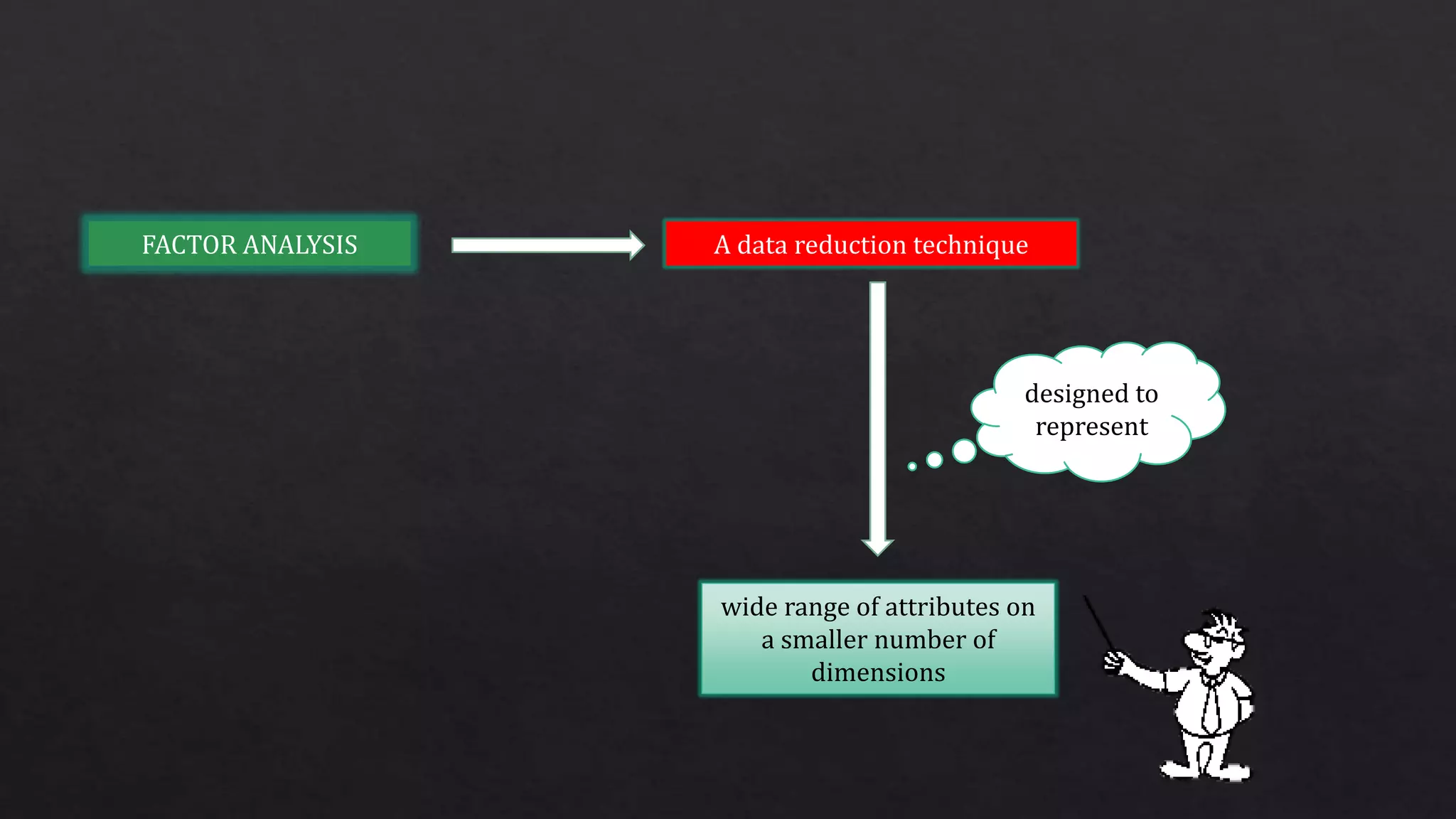
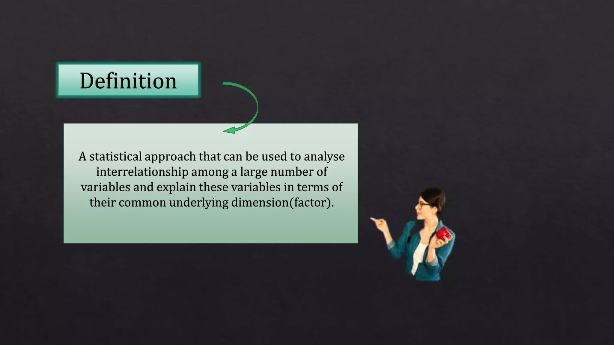
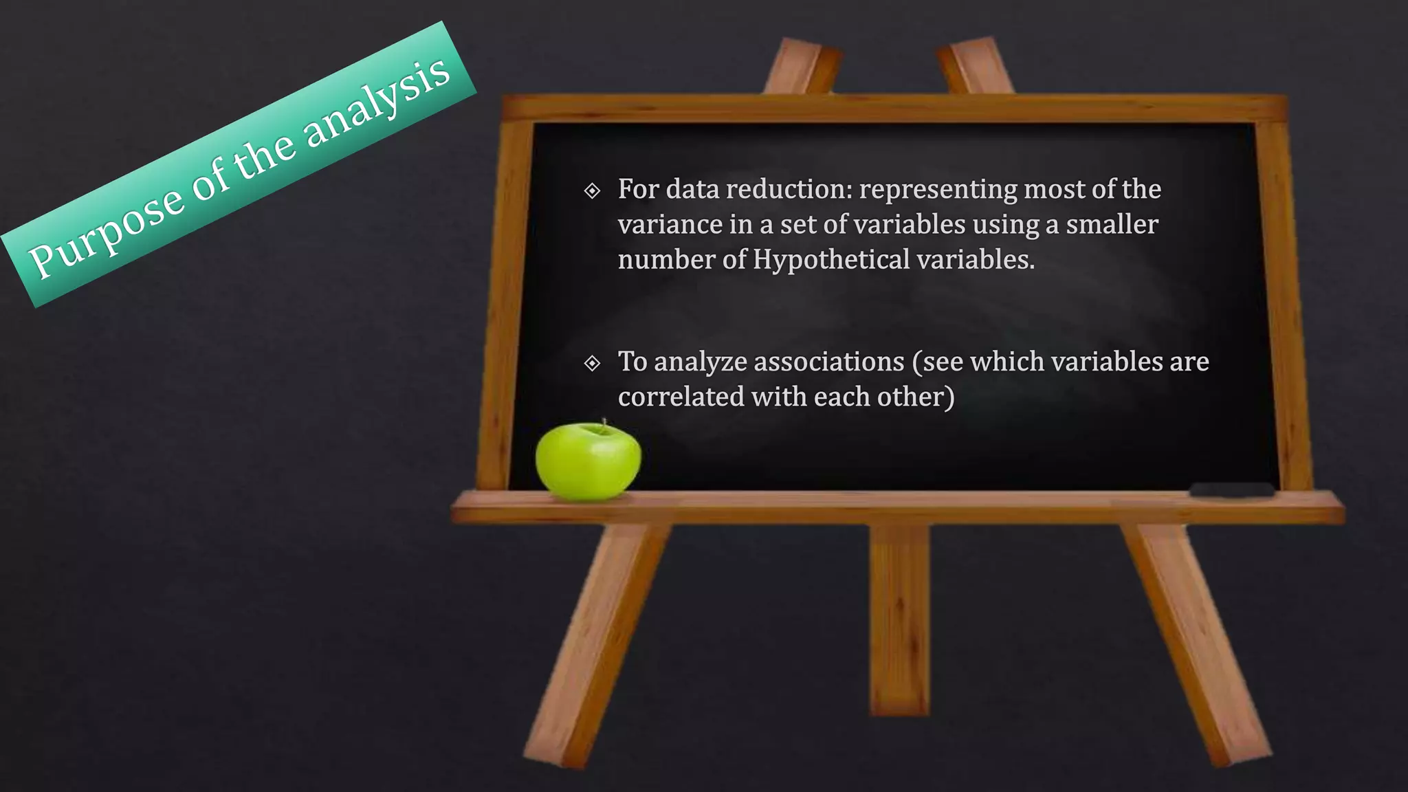
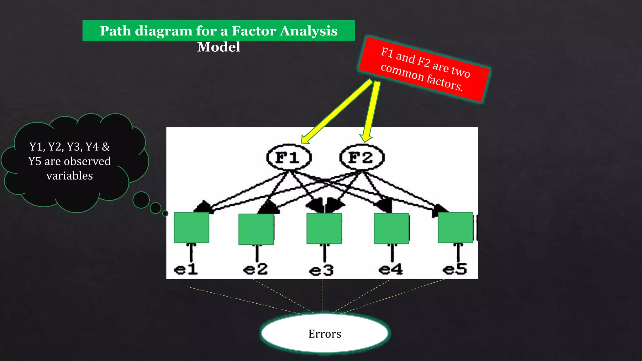
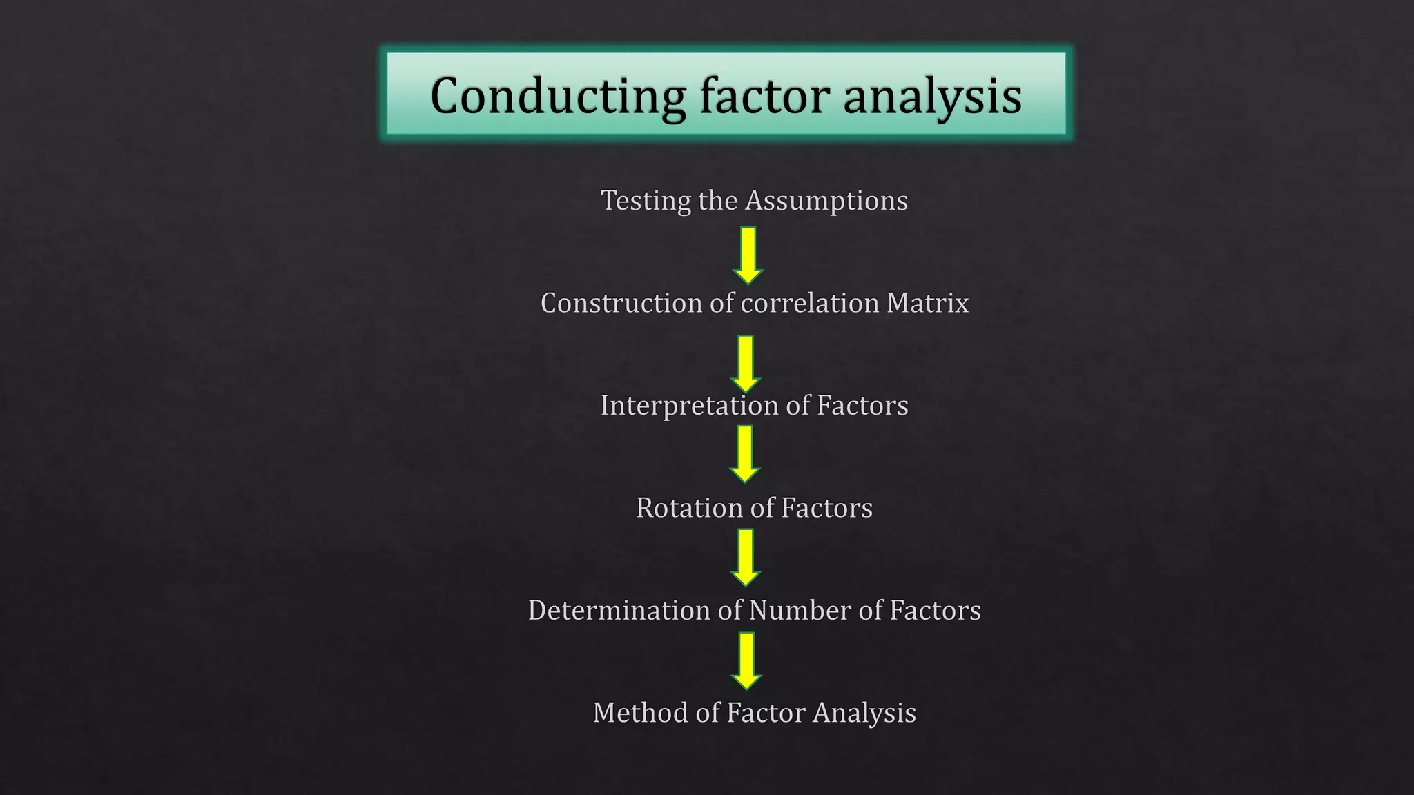
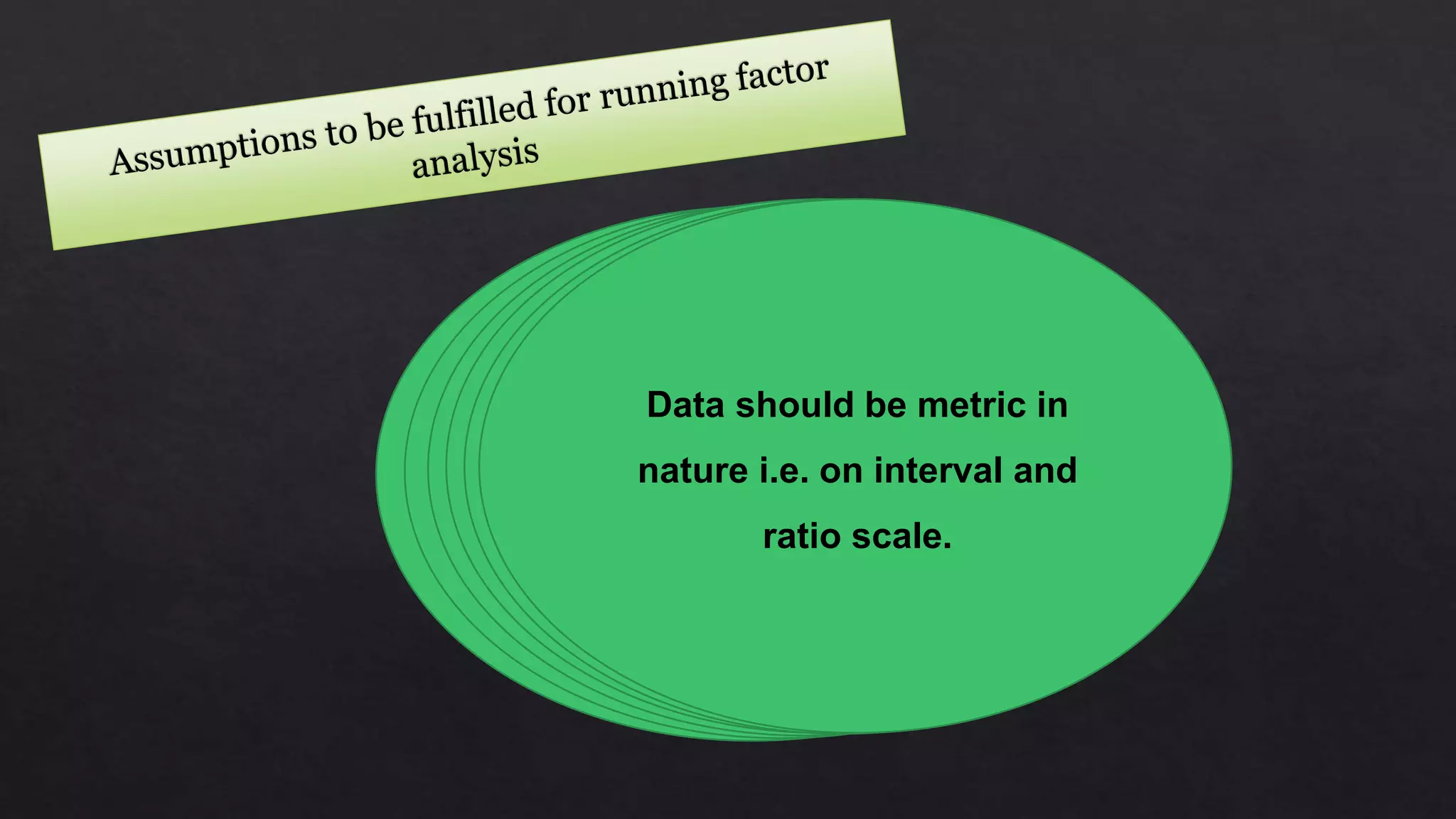
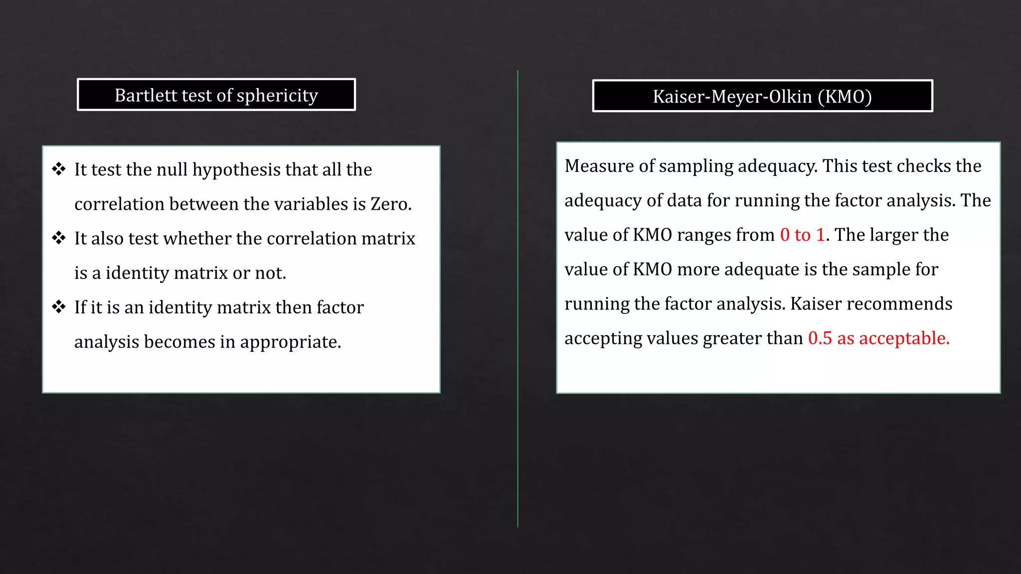
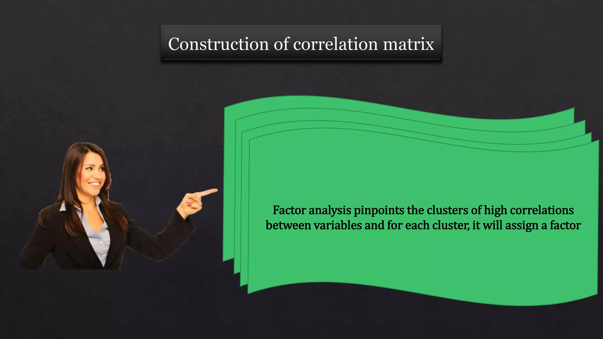
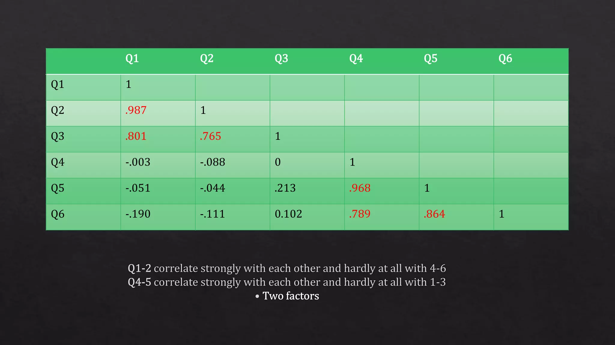
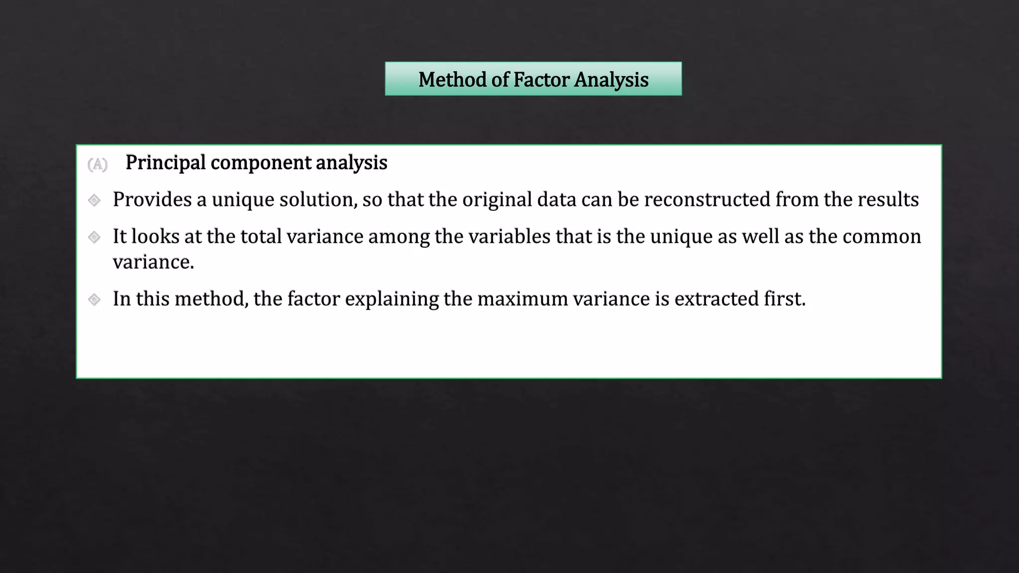
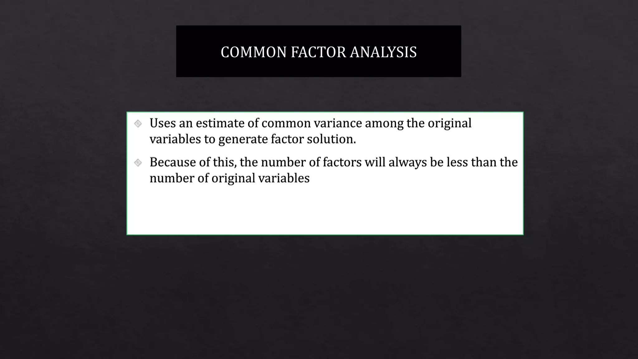
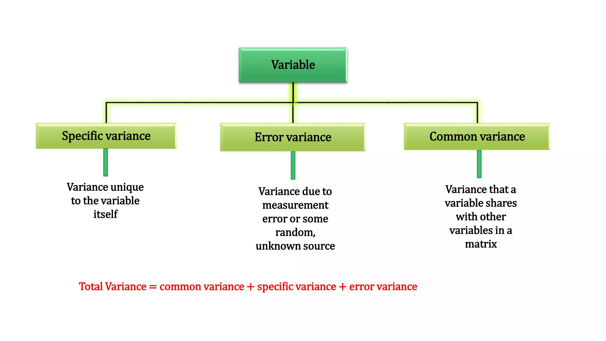
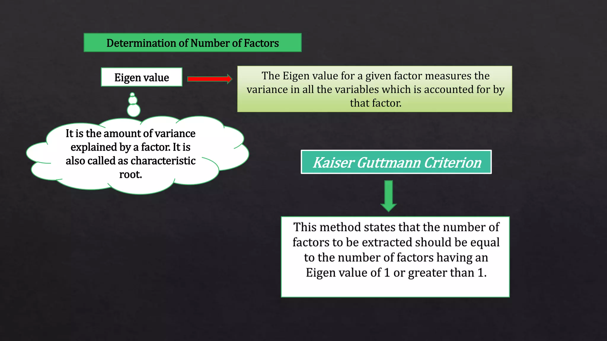
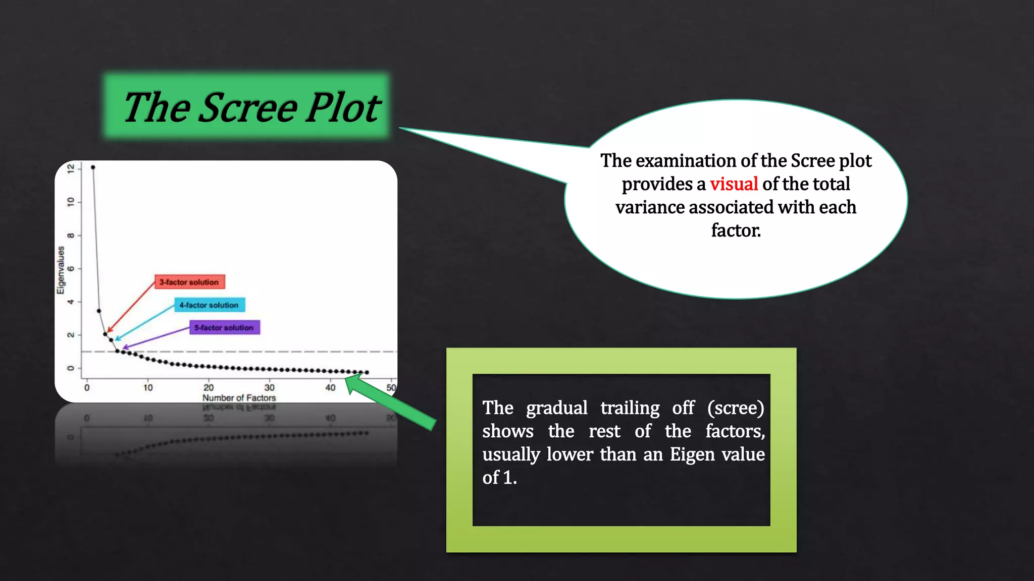
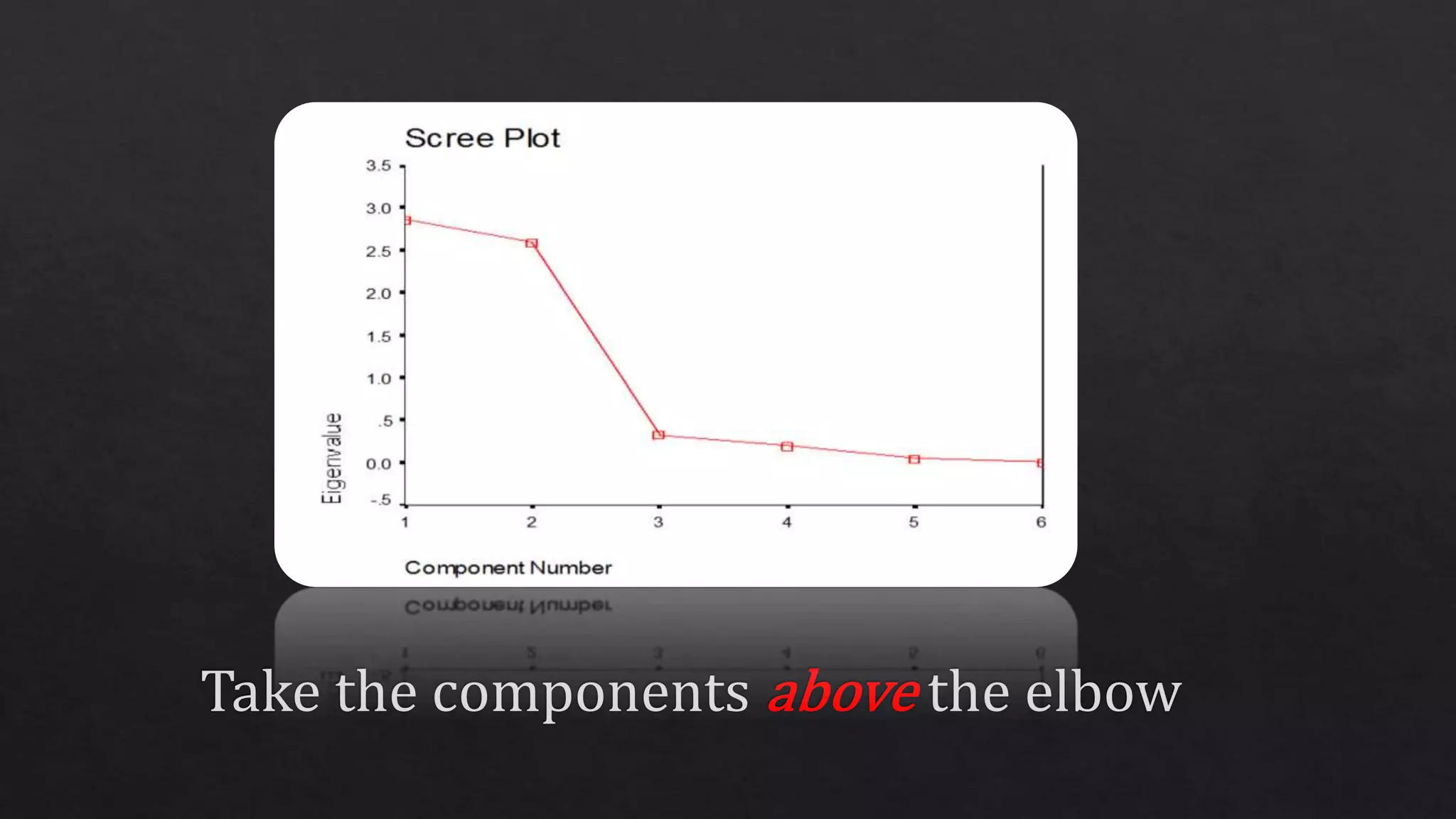
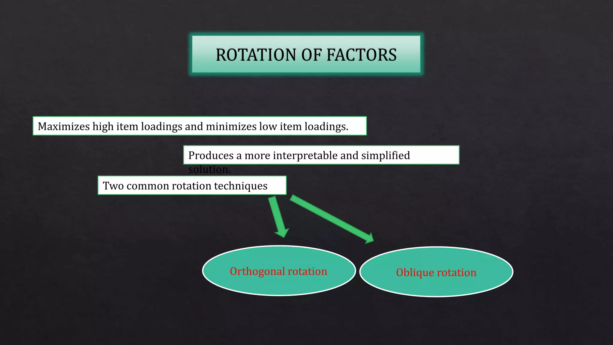
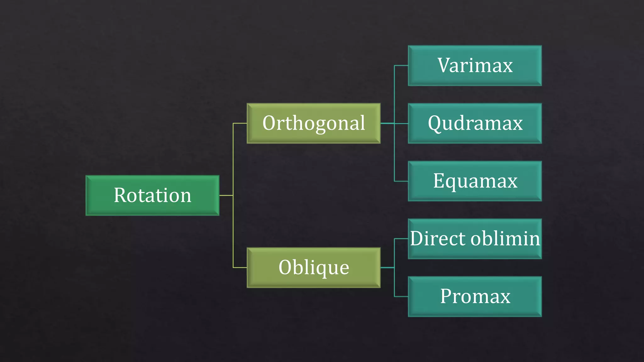
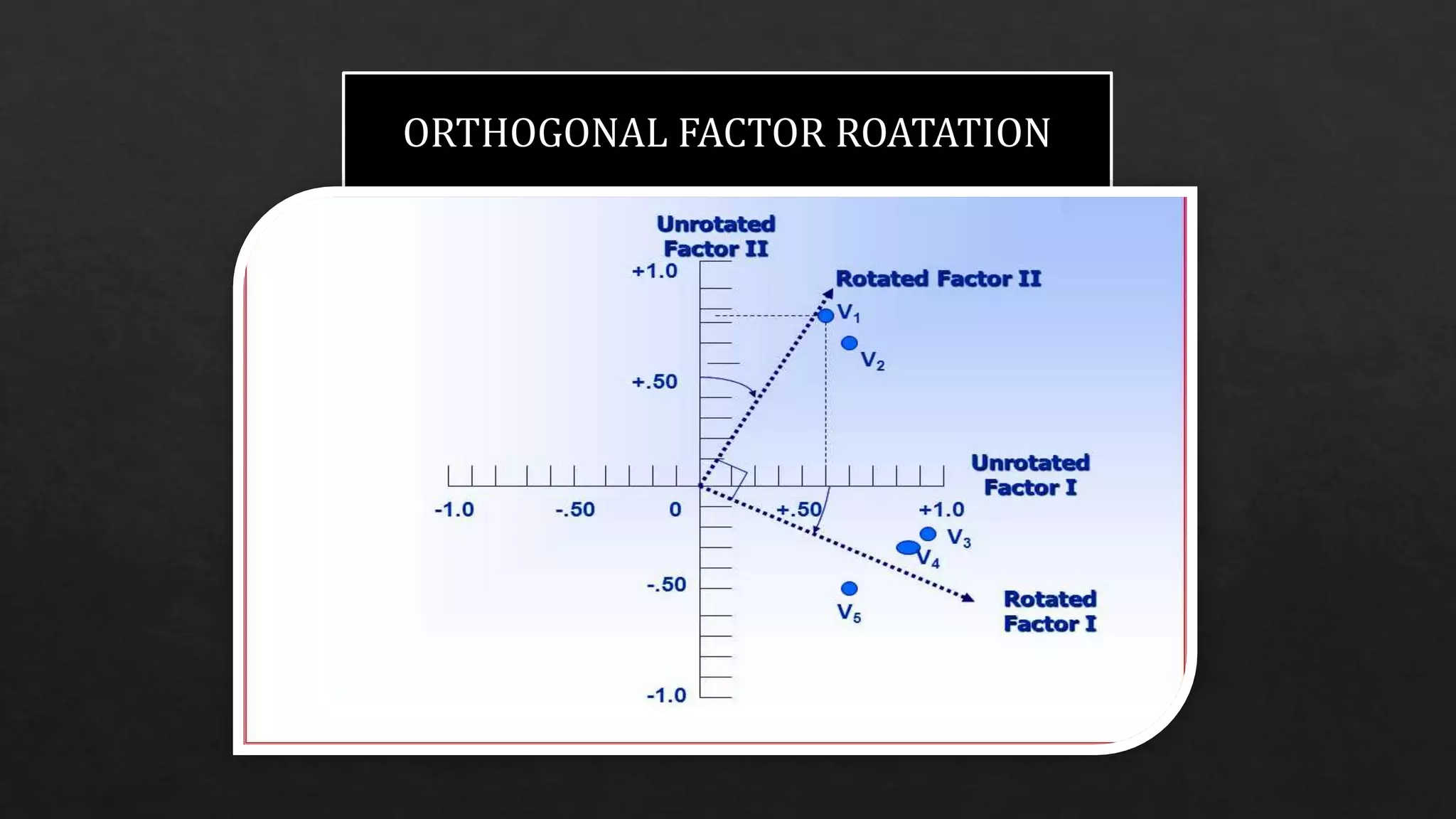
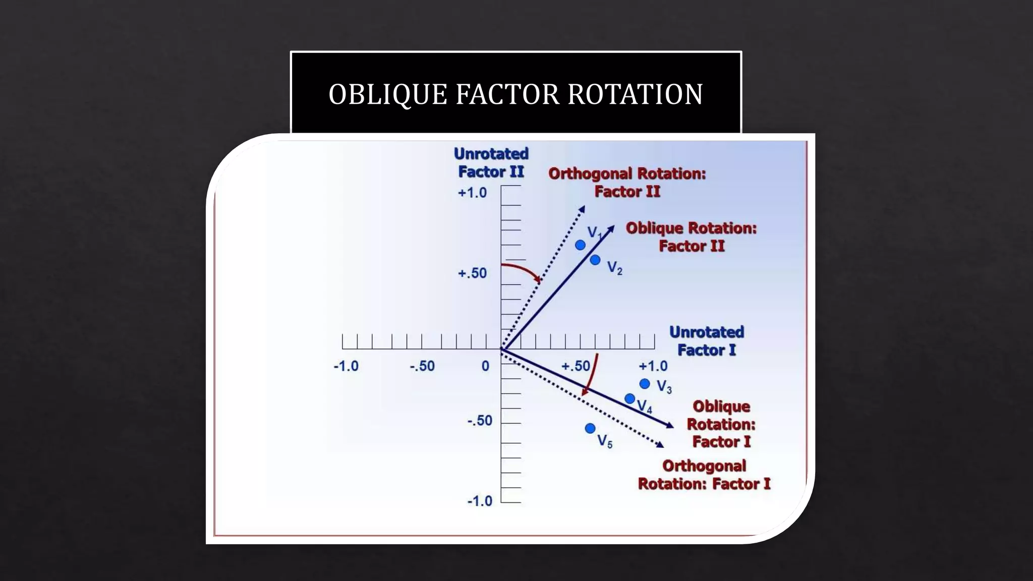
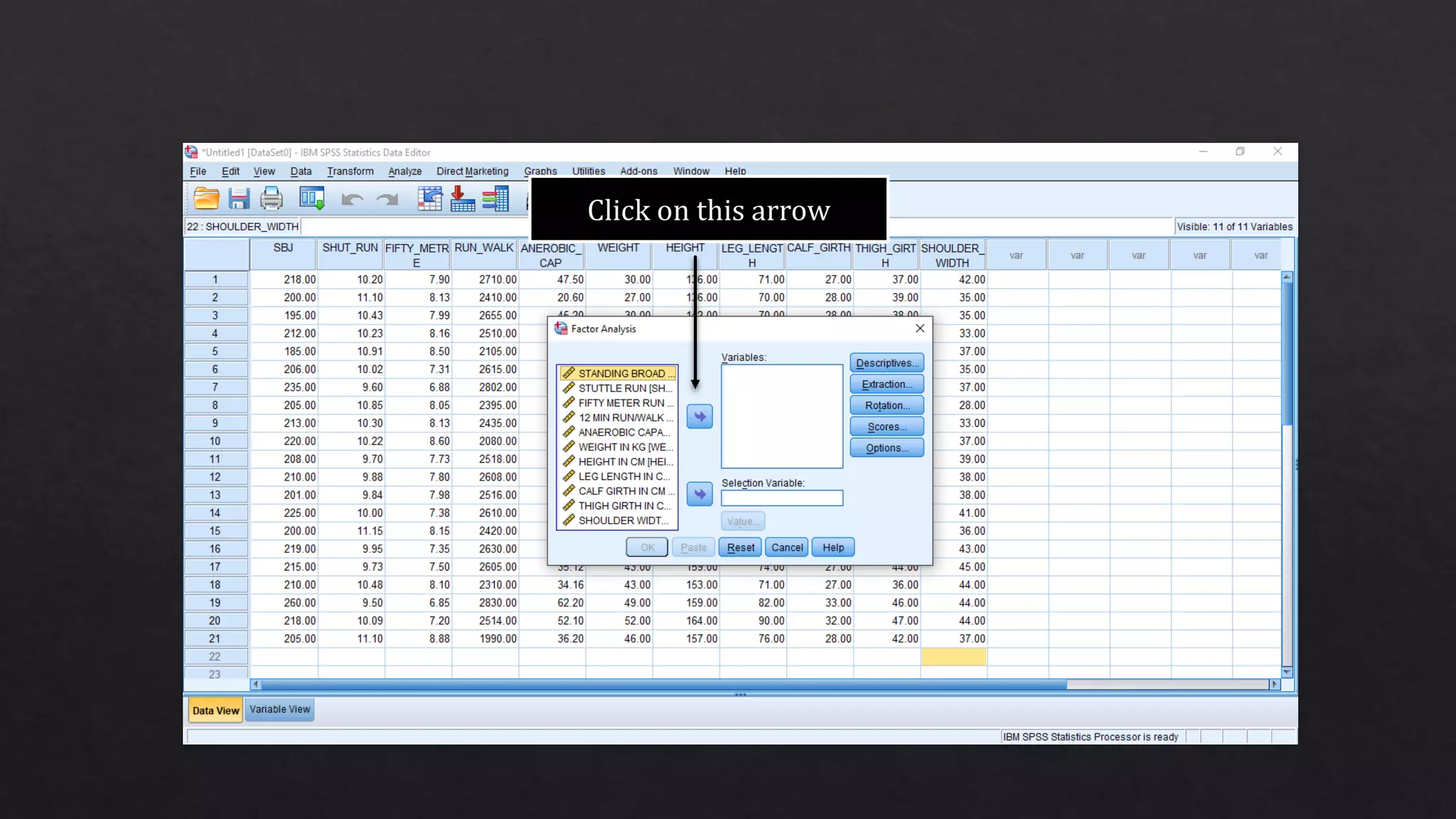
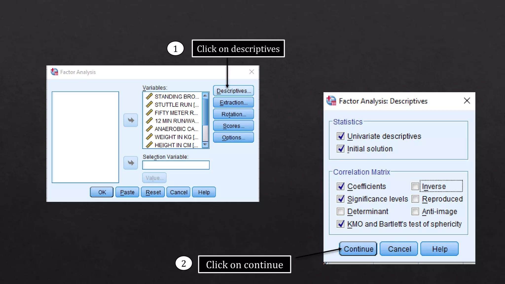
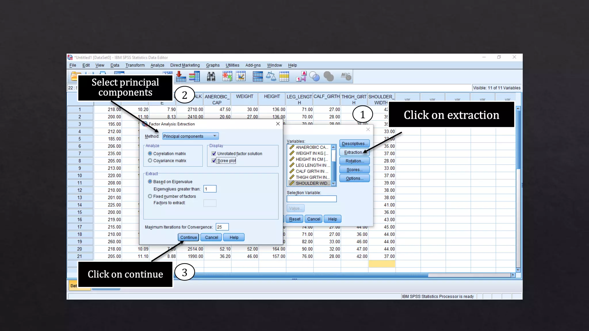
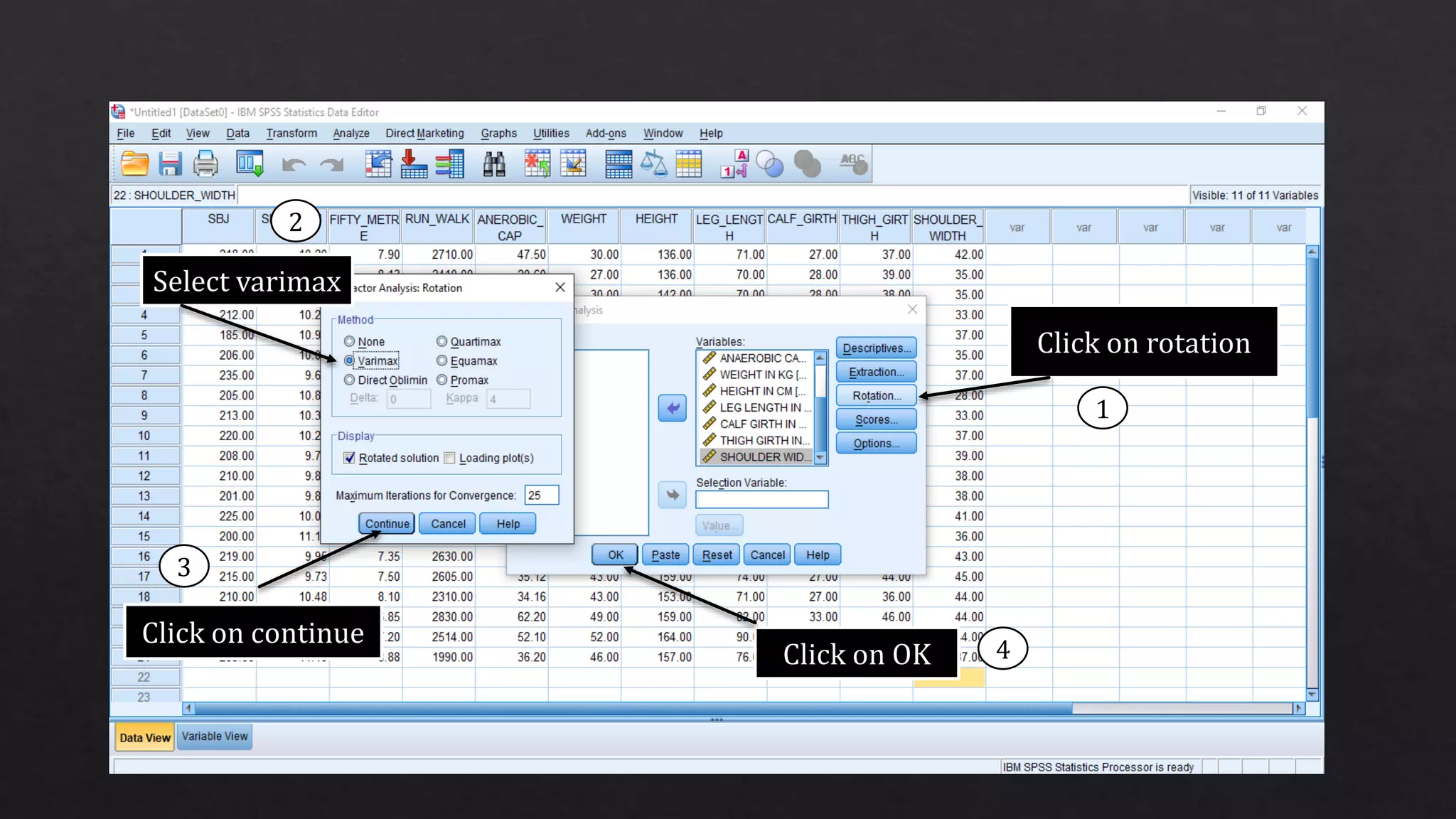
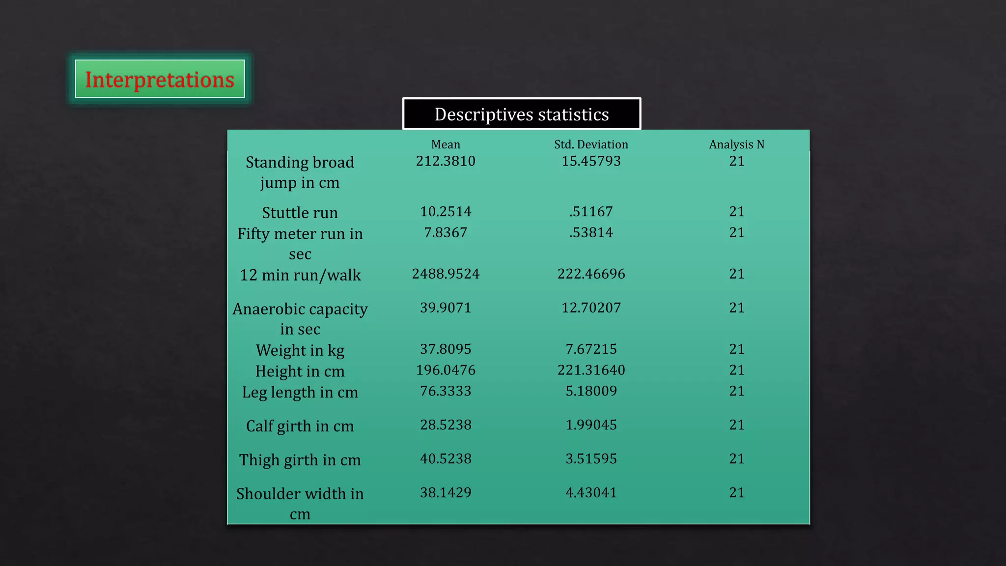
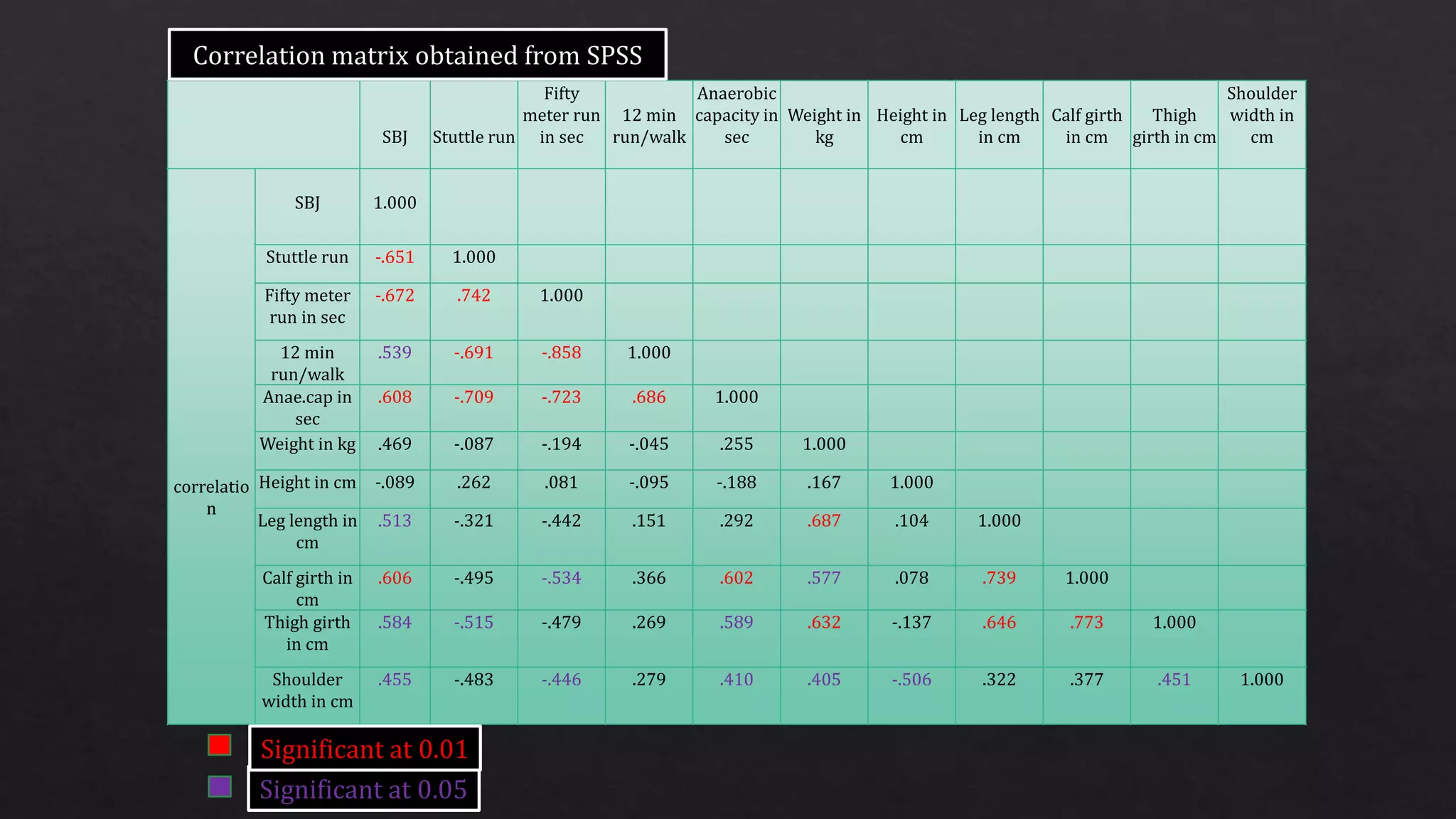
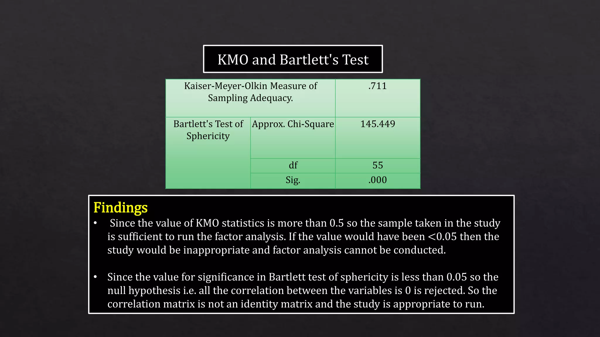
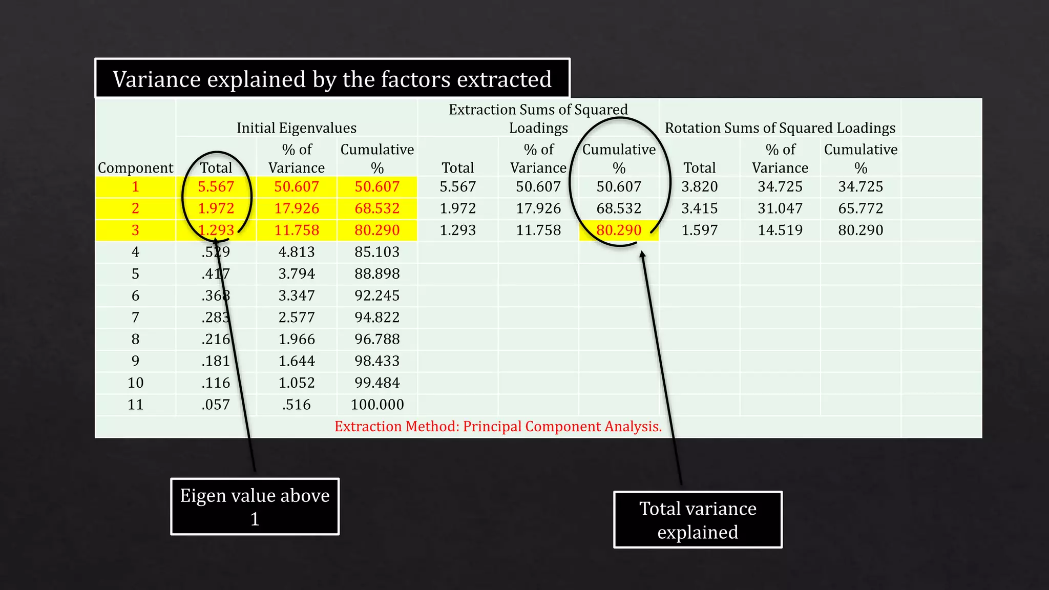
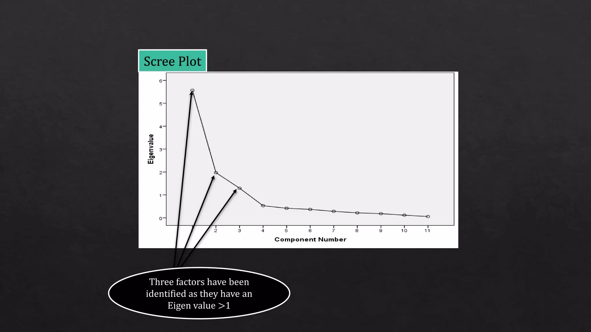
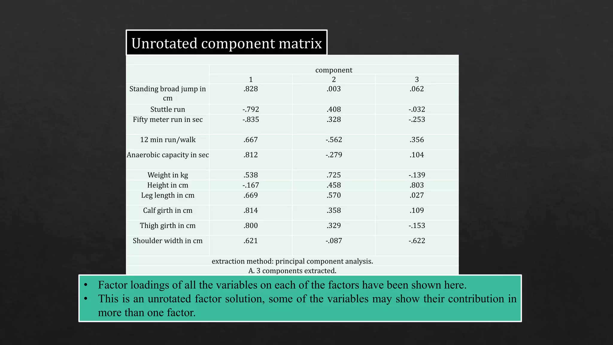
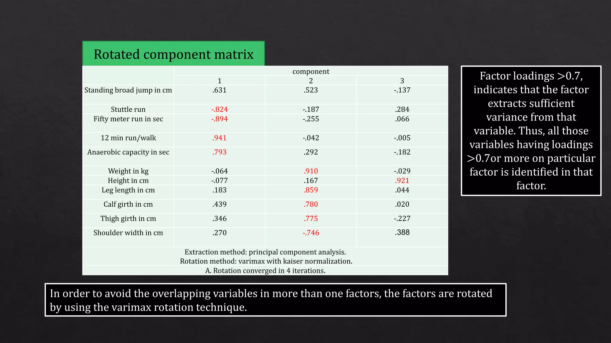
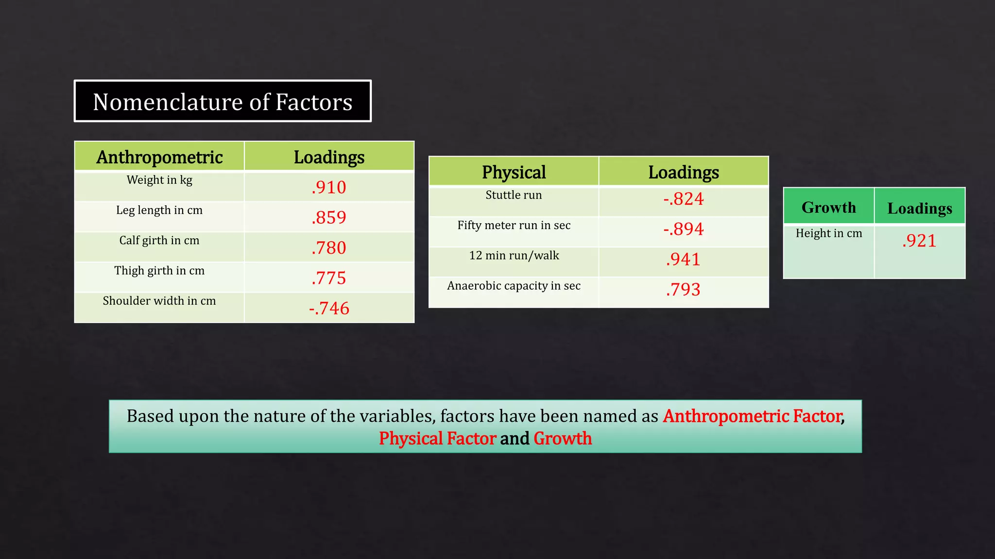
The document discusses factor analysis as a data reduction technique, detailing the requirements for conducting it, including variable properties and significance tests like the Kaiser-Meyer-Olkin measure and Bartlett's test of sphericity. It explains how to identify the number of factors using eigenvalues and rotation methods to achieve clearer factor loadings. The analysis results indicate sufficient sampling adequacy and highlight three factors that explain performance in various physical attributes related to sports.

3. FACTOR ANALYSIS A data reduction technique
wide range of attributes on
a smaller number of
dimensions
designed to
represent

7. Path diagram for a Factor Analysis
Model
Y1, Y2, Y3, Y4 &
Y5 are observed
variables
Errors

8. ?

10. No outliers in the data
set.
Normality of the data
set.
Multi collinearity and
singularity among the
variables does not exist.
Homoscedasticity does not
exist between the variables
because factor analysis is a
linear function of measured
variables.
Variables should be linear in
nature.
Data should be metric in
nature i.e. on interval and
ratio scale.

11. Measure of sampling adequacy. This test checks the
adequacy of data for running the factor analysis. The
value of KMO ranges from 0 to 1. The larger the
value of KMO more adequate is the sample for
running the factor analysis. Kaiser recommends
accepting values greater than 0.5 as acceptable.
Kaiser-Meyer-Olkin (KMO)
 It test the null hypothesis that all the
correlation between the variables is Zero.
 It also test whether the correlation matrix
is a identity matrix or not.
 If it is an identity matrix then factor
analysis becomes in appropriate.
Bartlett test of sphericity

12. Analyses the pattern of correlations between
variables in the correlation matrixWhich variables tend to correlate highly together?If variables are highly correlated, likely that they
represent the same underlying dimension
Factor analysis pinpoints the clusters of high correlations
between variables and for each cluster, it will assign a factor

13. Q1 Q2 Q3 Q4 Q5 Q6
Q1 1
Q2 .987 1
Q3 .801 .765 1
Q4 -.003 -.088 0 1
Q5 -.051 -.044 .213 .968 1
Q6 -.190 -.111 0.102 .789 .864 1

14. Method of Factor Analysis

16. Variable
Specific variance Error variance Common variance
Variance unique
to the variable
itself
Variance due to
measurement
error or some
random,
unknown source
Variance that a
variable shares
with other
variables in a
matrix
Total Variance = common variance + specific variance + error variance

17. Determination of Number of Factors
Eigen value The Eigen value for a given factor measures the
variance in all the variables which is accounted for by
that factor.
It is the amount of variance
explained by a factor. It is
also called as characteristic
root.
Kaiser Guttmann Criterion

18. The examination of the Scree plot
provides a visual of the total
variance associated with each
factor.
The gradual trailing off (scree)
shows the rest of the factors,
usually lower than an Eigen value
of 1.

20. Maximizes high item loadings and minimizes low item loadings.
Produces a more interpretable and simplified
solution.
Two common rotation techniques
Orthogonal rotation Oblique rotation

21. Rotation
Orthogonal
Varimax
Qudramax
Equamax
Oblique
Direct oblimin
Promax

24. Factor Loading Correlation coefficient between the variable
and the factor.
The squared factor loading of a variable indicates the
percentage variability explained by the factor in that
variable. A factor loading of 0.7 is considered to be
sufficient.

25. COMMUNALITY
The communality is the amount of variance each variable in the
analysis shares with other variables.
Squared multiple correlation for the variable as dependent using the
factors as predictors and is denoted by h².
The value of communality may be considered as the indicator of
reliability of a variable.

31. Variables

32. 1
2

33. 1
2
3

34. 1
2
3
4

35. Mean Std. Deviation Analysis N
Standing broad
jump in cm
212.3810 15.45793 21
Stuttle run 10.2514 .51167 21
Fifty meter run in
sec
7.8367 .53814 21
12 min run/walk 2488.9524 222.46696 21
Anaerobic capacity
in sec
39.9071 12.70207 21
Weight in kg 37.8095 7.67215 21
Height in cm 196.0476 221.31640 21
Leg length in cm 76.3333 5.18009 21
Calf girth in cm 28.5238 1.99045 21
Thigh girth in cm 40.5238 3.51595 21
Shoulder width in
cm
38.1429 4.43041 21
Descriptives statistics

36. SBJ Stuttle run
Fifty
meter run
in sec
12 min
run/walk
Anaerobic
capacity in
sec
Weight in
kg
Height in
cm
Leg length
in cm
Calf girth
in cm
Thigh
girth in cm
Shoulder
width in
cm
correlatio
n
SBJ 1.000
Stuttle run -.651 1.000
Fifty meter
run in sec
-.672 .742 1.000
12 min
run/walk
.539 -.691 -.858 1.000
Anae.cap in
sec
.608 -.709 -.723 .686 1.000
Weight in kg .469 -.087 -.194 -.045 .255 1.000
Height in cm -.089 .262 .081 -.095 -.188 .167 1.000
Leg length in
cm
.513 -.321 -.442 .151 .292 .687 .104 1.000
Calf girth in
cm
.606 -.495 -.534 .366 .602 .577 .078 .739 1.000
Thigh girth
in cm
.584 -.515 -.479 .269 .589 .632 -.137 .646 .773 1.000
Shoulder
width in cm
.455 -.483 -.446 .279 .410 .405 -.506 .322 .377 .451 1.000
Significant at 0.05
Significant at 0.01

37. Kaiser-Meyer-Olkin Measure of
Sampling Adequacy.
.711
Bartlett's Test of
Sphericity
Approx. Chi-Square 145.449
df 55
Sig. .000
Findings
• Since the value of KMO statistics is more than 0.5 so the sample taken in the study
is sufficient to run the factor analysis. If the value would have been <0.05 then the
study would be inappropriate and factor analysis cannot be conducted.
• Since the value for significance in Bartlett test of sphericity is less than 0.05 so the
null hypothesis i.e. all the correlation between the variables is 0 is rejected. So the
correlation matrix is not an identity matrix and the study is appropriate to run.

38. Component
Initial Eigenvalues
Extraction Sums of Squared
Loadings Rotation Sums of Squared Loadings
Total
% of
Variance
Cumulative
% Total
% of
Variance
Cumulative
% Total
% of
Variance
Cumulative
%
1 5.567 50.607 50.607 5.567 50.607 50.607 3.820 34.725 34.725
2 1.972 17.926 68.532 1.972 17.926 68.532 3.415 31.047 65.772
3 1.293 11.758 80.290 1.293 11.758 80.290 1.597 14.519 80.290
4 .529 4.813 85.103
5 .417 3.794 88.898
6 .368 3.347 92.245
7 .283 2.577 94.822
8 .216 1.966 96.788
9 .181 1.644 98.433
10 .116 1.052 99.484
11 .057 .516 100.000
Extraction Method: Principal Component Analysis.
Eigen value above
1
Total variance
explained

39. Three factors have been
identified as they have an
Eigen value >1

40. component
1 2 3
Standing broad jump in
cm
.828 .003 .062
Stuttle run -.792 .408 -.032
Fifty meter run in sec -.835 .328 -.253
12 min run/walk .667 -.562 .356
Anaerobic capacity in sec .812 -.279 .104
Weight in kg .538 .725 -.139
Height in cm -.167 .458 .803
Leg length in cm .669 .570 .027
Calf girth in cm .814 .358 .109
Thigh girth in cm .800 .329 -.153
Shoulder width in cm .621 -.087 -.622
extraction method: principal component analysis.
A. 3 components extracted.
• Factor loadings of all the variables on each of the factors have been shown here.
• This is an unrotated factor solution, some of the variables may show their contribution in
more than one factor.

41. component
1 2 3
Standing broad jump in cm .631 .523 -.137
Stuttle run -.824 -.187 .284
Fifty meter run in sec -.894 -.255 .066
12 min run/walk .941 -.042 -.005
Anaerobic capacity in sec .793 .292 -.182
Weight in kg -.064 .910 -.029
Height in cm -.077 .167 .921
Leg length in cm .183 .859 .044
Calf girth in cm .439 .780 .020
Thigh girth in cm .346 .775 -.227
Shoulder width in cm .270 -.746 .388
Extraction method: principal component analysis.
Rotation method: varimax with kaiser normalization.
A. Rotation converged in 4 iterations.
In order to avoid the overlapping variables in more than one factors, the factors are rotated
by using the varimax rotation technique.
Factor loadings >0.7,
indicates that the factor
extracts sufficient
variance from that
variable. Thus, all those
variables having loadings
>0.7or more on particular
factor is identified in that
factor.

42. Anthropometric Loadings
Weight in kg
.910
Leg length in cm
.859
Calf girth in cm
.780
Thigh girth in cm
.775
Shoulder width in cm
-.746
Physical Loadings
Stuttle run -.824
Fifty meter run in sec -.894
12 min run/walk .941
Anaerobic capacity in sec .793
Based upon the nature of the variables, factors have been named as Anthropometric Factor,
Physical Factor and Growth
Growth Loadings
Height in cm
.921

43. Variables Loadings
Weight in kg .910
Height in cm .921
Fifty meter run in sec -.894
12 min run/walk .941
Growth 0.921
Depending upon the sample data test battery for Badminton playing ability consists of
four variables.