This study reports the first weak-lensing detection of a large-scale filament funneling matter onto the core of the massive galaxy cluster MACSJ0717.5+3745. The analysis is based on Hubble Space Telescope images covering an area of 10x20 arcmin^2 around the cluster. A weak-lensing mass reconstruction detects the filament within 3 sigma and measures its projected length as ~4.5 h^-1 Mpc and mean density as (2.92±0.66)×10^8 h74 M⊙ kpc^-2. Assuming constraints on the filament's geometry based on galaxy velocities, the three-dimensional length is estimated to be 18 h^-1 M

1. Mon. Not. R. Astron. Soc. 000, 1–17 (XXXX) Printed 22 August 2012 (MN L TEX style file v2.2)
A
A Weak-Lensing Mass Reconstruction of the Large-Scale Filament
Feeding the Massive Galaxy Cluster MACSJ0717.5+3745
arXiv:1208.4323v1 [astro-ph.CO] 21 Aug 2012
Mathilde Jauzac,1,2⋆ Eric Jullo,1,3 Jean-Paul Kneib,1 Harald Ebeling,4 Alexie Leauthaud,5
Cheng-Jiun Ma,4 Marceau Limousin,1,6 Richard Massey,7 Johan Richard8
1 Laboratoire d’Astrophysique de Marseille - LAM, Universit´ d’Aix-Marseille & CNRS, UMR7326, 38 rue F. Joliot-Curie, 13388 Marseille Cedex 13, France
e
2 Astrophysics and Cosmology Research Unit, School of Mathematical Sciences, University of KwaZulu-Natal, Durban 4041, South Africa
3 Jet Propulsion Laboratory, California Institute of Technology, Pasadena, CA 91109, USA
4 Institute for Astronomy, University of Hawaii, 2680 Woodlawn Drive, Honolulu, Hawaii 96822, USA
5 Kavli Institute for the Physics and Mathematics of the Universe, Todai Institutes for Advanced Study, the University of Tokyo, Kashiwa, Japan 277-8583
(Kavli IPMU, WPI)
6 Dark Cosmology Centre, Niels Bohr Institute, University of Copenhagen, Juliane Maries Vej 30, DK-2100 Copenhagen, Denmark
7 Institute for Computational Cosmology, Durham University, South Road, Durham DH1 3LE, U.K.
8
CRAL, Observatoire de Lyon, Universit´ Lyon 1, 9 Avenue Ch. Andr´ , 69561 Saint Genis Laval Cedex, France
e e
Accepted 2012 August 20. Received 2012 August 15; in original form: 2012 April 27
ABSTRACT
We report the first weak-lensing detection of a large-scale filament funneling matter onto the
core of the massive galaxy cluster MACSJ0717.5+3745.
Our analysis is based on a mosaic of 18 multi-passband images obtained with the Ad-
vanced Camera for Surveys aboard the Hubble Space Telescope, covering an area of ∼ 10×20
arcmin2 . We use a weak-lensing pipeline developed for the COSMOS survey, modified for the
analysis of galaxy clusters, to produce a weak-lensing catalogue. A mass map is then com-
puted by applying a weak-gravitational-lensing multi-scale reconstruction technique designed
to describe irregular mass distributions such as the one investigated here. We test the result-
ing mass map by comparing the mass distribution inferred for the cluster core with the one
derived from strong-lensing constraints and find excellent agreement.
Our analysis detects the MACSJ0717.5+3745 filament within the 3 sigma detection con-
tour of the lensing mass reconstruction, and underlines the importance of filaments for the-
oretical and numerical models of the mass distribution in the Cosmic Web. We measure the
filament’s projected length as ∼ 4.5 h−1 Mpc, and its mean density as (2.92±0.66)×108 h74 M⊙
74
kpc−2 . Combined with the redshift distribution of galaxies obtained after an extensive spectro-
scopic follow-up in the area, we can rule out any projection effect resulting from the chance
alignment on the sky of unrelated galaxy group-scale structures. Assuming plausible con-
straints concerning the structure’s geometry based on its galaxy velocity field, we construct a
3D model of the large-scale filament. Within this framework, we derive the three-dimensional
length of the filament to be 18 h−1 Mpc. The filament’s deprojected density in terms of the
74
critical density of the Universe is measured as (206 ± 46) × ρcrit , a value that lies at the very
high end of the range predicted by numerical simulations. Finally, we study the distribution
of stellar mass in the field of MACSJ0717.5+3749 and, adopting a mean mass-to-light ratio
M∗ /LK of 0.73 ± 0.22 and assuming a Chabrier Initial-Mass Function, measure a stellar
mass fraction along the filament of (0.9 ± 0.2)%, consistent with previous measurements in
the vicinity of massive clusters.
Key words: cosmology: observations - gravitational lensing - large-scale structure of Uni-
verse
1 INTRODUCTION
In a Universe dominated by Cold Dark Matter (CDM), such as
⋆ E-mail: mathilde.jauzac@gmail.com (MJ) the one parameterised by the ΛCDM concordance cosmology, hi-

2. 2 M. Jauzac, E. Jullo, J.-P. Kneib, H. Ebeling, A. Leauthaud, C. J. Ma, M. Limousin, R. Massey, J. Richard
erarchical structure formation causes massive galaxy clusters to
form through a series of successive mergers of smaller clusters
and groups of galaxies, as well as through continuous accretion
of surrounding matter. N-body simulations of the dark-matter dis-
tribution on very large scales (Bond et al. 1996; Yess & Shandarin
1996; Arag´ n-Calvo et al. 2007; Hahn et al. 2007) predict that
o
these processes of merging and accretion occur along preferred di-
rections, i.e., highly anisotropically. The result is the “cosmic web”
(Bond et al. 1996), a spatially highly correlated structure of inter-
connected filaments and vertices marked by massive galaxy clus-
ters. Abundant observational support for this picture has been pro-
vided by large-scale galaxy redshift surveys (e.g., Geller & Huchra
1989; York et al. 2000; Colless et al. 2001) showing voids sur-
rounded and connected by filaments and sheets of galaxies.
A variety of methods have been developed to detect filaments
in surveys, among them a “friends of friends” algorithm (FOF,
Huchra & Geller 1982) combined with “Shapefinders” statistics
(Sheth & Jain 2003); the “Skeleton” algorithm (Novikov et al.
2006; Sousbie et al. 2006); a two-dimensional technique developed
by Moody et al. (1983); and the Smoothed Hessian Major Axis Fil-
ament Finder (SHMAFF, Bond et al. 2010).
Figure 1. Area of our spectroscopic survey of MACSJ0717.5+3745. Out-
Although ubiquitous in large-scale galaxy surveys, filaments
lined in red is the region covered by our Keck/DEIMOS masks; outlined
have proven hard to characterise physically, owing to their low in blue is the area observed with HST/ACS. Small circles correspond to
density and the fact that the best observational candidates often objects for which redshifts were obtained; large filled circles mark cluster
turn out to be not primordial in nature but the result of recent members. The black contours show the projected galaxy density (see Ma et
cluster mergers. Specifically, attempts to study the warm-hot in- al. 2008).
tergalactic medium (WHIM, Cen & Ostriker 1999), resulting from
the expected gravitational heating of the intergalactic medium in
filaments, remain largely inconclusive because it is hard to ascer- gaps between CCD chips. Indeed, Gavazzi et al. (2004) showed
tain for filaments near cluster whether spectral X-ray features orig- the detection to have been spurious by means of a second study
inate from the filament or from past or ongoing clusters merg- of MS0302+17 using the CFHT12K camera. A weak gravitational
ers (Kaastra et al. 2006; Rasmussen 2007; Galeazzi et al. 2009; lensing analysis with MPG/ESO Wide Field Imager conducted by
Williams et al. 2010). Some detections appear robust as they have Gray et al. (2002) claimed the detection of a filament in the triple
been repeatedly confirmed (Fang et al. 2002, 2007; Williams et al. cluster A901/902. The candidate filament appeared to connect two
2007) but are based on just one X-ray line. An alternative observa- of the clusters and was detected in both the galaxy distribution and
tional method is based on a search for filamentary overdensities of in the weak-lensing mass map. However, this detection too was
galaxies relative to the background (Pimbblet & Drinkwater 2004; of low significance and coincided partly with a gap between two
Ebeling et al. 2004). When conducted in 3D, i.e., including spec- chips of the camera. As in the case of MS0302+17, a re-analysis of
troscopic galaxy redshifts, this method is well suited to detecting the A901/A902 complex using high-quality HST/ACS images by
filament candidates. It does, however, not allow the determination Heymans et al. (2008) failed to detect the filament and led the au-
of key physical properties unless it is supplemented by follow-up thors to conclude that the earlier detection was caused by residual
studies targeting the presumed WHIM and dark matter which are PSF systematics and limitation of the KS93 mass reconstruction
expected to constitute the vast majority of the mass of large-scale used in the study by Gray et al. (2002). A further detection of a
filaments. By contrast, weak gravitational lensing offers the tan- filament candidate was reported by Dietrich et al. (2005) based on
talising possibility of detecting directly the total mass content of a weak gravitational lensing analysis of the close double cluster
filaments (Mead et al. 2010), since the weak-lensing signal arises A222/A223. However, as in other similar cases, the proximity of
from luminous and dark matter alike, regardless of its dynamical the two clusters connected by the putative filament raises the pos-
state. sibility of the latter being a merger remnant rather than primordial
Previous weak gravitational lensing studies of binary clusters in nature.
found tentative evidence of filaments, but did not result in clear de- In this paper we describe the first weak gravitational analy-
tections. One of the first efforts was made by Clowe et al. (1998) sis of the very massive cluster MACSJ0717.5+3745 (z = 0.55;
who reported the detection of a filament apparently extending from Edge et al. 2003; Ebeling et al. 2004, 2007; Ma et al. 2008, 2009).
the distant cluster RX J1716+67 (z = 0.81), using images obtained Optical and X-ray analyses of the system (Ebeling et al. 2004;
with the Keck 10m telescope and University of Hawaii (UH) 2.2m Ma et al. 2008, 2009) find compelling evidence of a filamentary
telescope. This filamentary structure would relate two distinct sub structure extending toward the South-East of the cluster core. Us-
clusters detected on the mass and light maps. The detection was ing weak-lensing data to reconstruct the mass distribution in and
not confirmed though. Almost at the same time Kaiser et al. (1998) around MACSJ0717.5+3745, we directly detect the reported fila-
conducted a weak lensing study of the supercluster MS0302+17 mentary structure in the field of MACSJ0717.5+3745.
with the UH8K CCD camera on the Canada France Hawaii Tele- The paper is organized as follows. After an overview of
scope (CFHT). Their claimed detection of a filament in the field the observational data in Section 2, we discuss the gravitational
was, however, questioned on the grounds that the putative fila- lensing data in hand in Section 3. The modeling of the mass
ment overlapped with both a foreground structure as well as with using a multi-scale approach is described in Section 4. Results are

3. The Large-Scale Filament Feeding MACSJ0717.5+3745 3
Table 1. Overview of the HST/ACS observations of MACSJ0717.5+3745. *: Cluster core; observed through F555W, rather than F606W filter.
F606W F814W
R.A. (J2000) Dec (J2000) Date Exposure Time (s) Date Exposure Time (s) Programme ID
07 17 32.93 +37 45 05.4 2004-04-02* 4470* 2004-04-02 4560 9722
07 17 31.81 +37 49 20.6 2005-02-08 1980 2005-02-08 4020 10420
07 17 20.38 +37 47 07.5 2005-01-27 1980 2005-01-27 4020 10420
07 17 08.95 +37 44 54.3 2005-01-27 1980 2005-01-27 4020 10420
07 17 43.23 +37 47 03.1 2005-01-30 1980 2005-01-30 4020 10420
07 17 20.18 +37 42 38.8 2005-02-01 1980 2005-02-01 4020 10420
07 17 54.26 +37 44 49.3 2005-01-27 1980 2005-01-27 4020 10420
07 17 42.82 +37 42 36.3 2005-01-24 1980 2005-01-25 4020 10420
07 17 31.39 +37 40 23.3 2005-02-01 1980 2005-02-01 4020 10420
07 18 05.46 +37 42 33.6 2005-02-04 1980 2005-02-04 4020 10420
07 17 54.02 +37 40 20.6 2005-02-04 1980 2005-02-04 4020 10420
07 17 42.79 +37 38 05.7 2005-02-05 1980 2005-02-05 4020 10420
07 18 16.65 +37 40 17.7 2005-02-05 1980 2005-02-05 4020 10420
07 18 05.22 +37 38 04.9 2005-02-05 1980 2005-02-05 4020 10420
07 17 53.79 +37 35 52.0 2005-02-05 1980 2005-02-05 4020 10420
07 18 27.84 +37 38 01.9 2005-02-08 1980 2005-02-08 4020 10420
07 18 16.40 +37 35 49.1 2005-02-08 1980 2005-02-08 4020 10420
07 18 04.97 +37 33 36.2 2005-02-09 1980 2005-02-09 4020 10420
discussed in Section 5, and we present our conclusions in Section 6. Table 2. Overview of groundbased imaging observations of
MACSJ0717.5+3745.
All our results use the ΛCDM concordance cosmology with
ΩM = 0.3, ΩΛ = 0.7, and a Hubble constant H0 = 74 km s−1 Mpc−1 ,
hence 1” corresponds to 6.065 kpc at the redshift of the cluster. Subaru CFHT
Magnitudes are quoted in the AB system. B V RC IC z’ u* J KS
Exposure (hr) 0.4 0.6 0.8 0.4 0.5 1.9 1.8 1.7
Seeing (arcsec) 0.8 0.7 1.0 0.8 0.6 1.0 0.9 0.7
2 OBSERVATIONS
The MAssive Cluster Survey (MACS, Ebeling et al. 2001) was the
first cluster survey to search exclusively for very massive clusters
at moderate to high redshift. Covering over 20,000 deg2 and us-
ing dedicated optical follow-up observations to identify faint X-
ray sources detected in the ROSAT All-Sky Survey, MACS com-
piled a sample of over 120 very X-ray luminous clusters at z > 0.3, February 9, 2005, with the ACS aboard HST (GO-10420, PI Ebel-
thereby more than tripling the number of such systems previously ing). The 3×6 mosaic consists of images in the F606W and F814W
known. The high-redshift MACS subsample (Ebeling et al. 2007) filters, observed for roughly 2.0 ks and 4.0 ks respectively (1 & 2
comprises 12 clusters a z > 0.5. MACSJ0717.5+3745 is one of HST orbits). Only 17 of the 18 tiles of the mosaic were covered
them. All 12 were observed with the ACIS-I imaging spectrograph though, since the core of the cluster had been observed already (see
onboard the Chandra X-ray Observatory. Moderately deep optical Tab. 1 for more details).
images covering 30 × 27 arcmin2 were obtained in five passbands Charge Transfer Inefficiency (CTI), due to radiation damage
(B, V, R, I, z′ ) with the SuprimeCam wide-field imager on the of the ACS CCDs above the Earth’s atmosphere, creates spurious
Subaru 8.2m Telescope, and supplemented with u-band imaging trails behind objects in HST/ACS images. Since CTI affects galaxy
obtained with MegaCam on the Canada France Hawaii Telescope photometry, astrometry, and shape measurements, correcting the ef-
(CFHT). Finally, the cores of all clusters in this MACS subsam- fect is critical for weak-lensing studies. We apply the algorithm
ple were observed with the Advanced Camera for Surveys (ACS) proposed by Massey et al. (2010) which operates on the raw data
onboard HST in two bands, F555W & F814W, for 4.5ks in both and returns individual electrons to the pixels from which they were
bands, as part of programmes GO-09722 and GO-11560 (PI Ebel- erroneously dragged during readout. Image registration, geometric
ing). distortion corrections, sky subtraction, cosmic ray rejection, and the
final combination of the dithered images are then performed using
the standard MULTIDRIZZLE routines (Koekemoer et al. 2002).
MULTIDRIZZLE parameters are set to values optimised for pre-
2.1 HST/ACS Wide-Field Imaging
cise galaxy shape measurement (Rhodes et al. 2007), and output
A mosaic of images of MACSJ0717.5+3745 and the filamentary images created with a 0.03” pixel grid, compared to the native ACS
structure to the South-East was obtained between January 24 and pixel scale of 0.05”.

4. 4 M. Jauzac, E. Jullo, J.-P. Kneib, H. Ebeling, A. Leauthaud, C. J. Ma, M. Limousin, R. Massey, J. Richard
4
BRI selection BRI Redshift Distribution
All galaxies before BRI selection
Foreground galaxies (zphot) 250 after BRI selection
Cluster galaxies (zphot)
Foreground & Cluster galaxies (zspec)
3 200
Number of galaxies
MAGB −MAGRc
150
2
100
1 50
0
0.0 0.5 1.0 1.5 0.2 0.4 0.6 0.8 1.0 1.2 1.4
MAGRc − MAGIc z
Figure 2. Colour-colour diagram (B−R vs R−I) for objects within the Figure 3. Redshift distribution of all galaxies with B, Rc , and Ic photometry
HST/ACS mosaic of MACSJ0717.5+3745. Grey dots represent all objects from Subaru/SuprimeCam observations that have photometric or spectro-
in the study area. Unlensed galaxies diluting the shear signal are marked by scopic redshifts (black histogram). The cyan histogram shows the redshift
different colours: galaxies spectroscopically confirmed as cluster members distribution of galaxies classified as background objects using the BRI cri-
or foreground galaxies (green); galaxies classified as foreground objects be- terion illustrated in Fig. 2.
cause of their photometric redshifts (red); and galaxies classified as cluster
members via photometric redshifts (yellow). The solid black lines delin-
eate the BRI colour-cut defined for this work to mitigate shear dilution by
unlensed galaxies. 2.3 Spectroscopic and Photometric Redshifts
Spectroscopic observations of MACSJ0717.5+3745 (including the
full length of the filament) were conducted between 2000 and 2008,
mainly with the DEIMOS spectrograph on the Keck-II 10m tele-
scope on Mauna Kea, supplemented by observations of the cluster
2.2 Groundbased Imaging core region performed with the LRIS and GMOS spectrographs on
Keck-I and Gemini-North, respectively. The DEIMOS instrument
MACSJ0717.5+3745 was observed in the B, V, Rc , Ic and z′ bands setup combined the 600ZD grating with the GC455 order-blocking
with the Suprime-Cam wide-field camera on the Subaru 8.2m tele- filter and a central wavelength between 6300 and 7000 Å; the expo-
scope (Miyazaki et al. 2002). These observations are supplemented sure time per MOS (multi-object spectroscopy) mask was typically
by images in the u* band obtained with the MegaPrime camera on 3×1800 s. A total of 18 MOS masks were used in our DEIMOS
the CFHT 3.6m telescope, as well as near-infrared imaging in the observations; spectra of 1752 unique objects were obtained (65 of
J and KS bands obtained with WIRcam on CFHT. Exposure times them with LRIS, and 48 with GMOS), yielding 1079 redshifts, 537
and seeing conditions for these observations are listed in Tab. 2 of them of cluster members. Figure 1 shows the area covered by
(see also C.-J. Ma, Ph.D. thesis). All data were reduced using stan- our spectroscopic survey as well as the loci of the targeted galax-
dard techniques which were, however, adapted to deal with special ies. The data were reduced with the DEIMOS pipeline developed
characteristics of the Suprime-Cam and MegaPrime data; for more by the DEEP2 project.
details see Donovan (2007). Photometric redshifts for galaxies with mRc <24.0 were com-
The groundbased imaging data thus obtained are used primar- puted using the adaptive SED-fitting code Le Phare (Arnouts et al.
ily to compute photometric redshifts which allow the elimination 1999; Ilbert et al. 2006, 2009). In addition to employing χ2 opti-
of cluster members and foreground galaxies that would otherwise mization during SED fitting, Le Phare adaptively adjusts the pho-
dilute the shear signal. To this end we use the object catalogue com- tometric zero points by using galaxies with spectroscopic redshifts
piled by Ma et al. (2008) which we describe briefly in the follow- as a training set. This approach reduces the fraction of catastrophic
ing. Imaging data from the passbands listed in Tab. 2 were seeing- errors and also mitigates systematic trends in the differences be-
matched using the technique described in Kartaltepe et al. (2008) tween spectroscopic and photometric redshifts (Ilbert et al. 2006).
in order to allow a robust estimate of the spectral energy distribu- Further details, e.g. concerning the selection of targets for
tion (SED) for all objects within the field of view. The object cata- spectroscopy or the spectral templates used for the determination
logue was then created using the SExtractor photometry package of photometric redshifts, are provided by Ma et al. (2008). The full
(Bertin & Arnouts 1996) in ”dual mode” using the R-band image as redshift catalogue as well as an analysis of cluster substructure and
the reference detection image. More details are given in Ma et al. dynamics as revealed by radial velocities will be presented in Ebel-
(2008). ing et al. (2012, in preparation).

5. The Large-Scale Filament Feeding MACSJ0717.5+3745 5
3.0
uBV selection uBV Redshift Distribution
All galaxies before uBV selection
Foregound galaxies (zphot) 250 after uBV selection
Cluster galaxies (zphot)
2.5 Foreground & Cluster galaxies (zspec)
200
2.0
Number of galaxies
MAGB −MAGV
150
1.5
100
1.0
0.5 50
0.0 0
−0.5 0.0 0.5 1.0 1.5 0.2 0.4 0.6 0.8 1.0 1.2 1.4
MAGu − MAGB z
Figure 4. As Fig. 2 but for the B−V and u−B colours. The solid black Figure 5. Redshift distribution of all galaxies with u, B, and V photome-
line delineates the uBV colour-cut defined for this work to mitigate shear try from CFHT/MegaCam and Subaru/SuprimeCam observations that have
dilution by unlensed galaxies. photometric or spectroscopic redshifts (black histogram). The cyan his-
togram shows the redshift distribution of galaxies classified as background
objects using the uBV criterion illustrated in Fig. 4.
3 WEAK GRAVITATIONAL LENSING ANALYSIS
3.1 The ACS catalogue all quantities derived from it. Identifying and eliminating as many
Our weak-lensing analysis is based on shape measurements in the of the contaminating unlensed galaxies is thus critical.
ACS/F814W band. Following a method developed for the anal- As a first step, we identify cluster galaxies with the help
ysis of data obtained for the COSMOS survey and described in of the catalogue of photometric and spectroscopic redshifts com-
Leauthaud et al. (2007) (hereafter L07) we use the SExtractor piled by Ma et al. (2008) from groundbased observations of the
photometry package (Bertin & Arnouts 1996) to detect sources in MACSJ0717.5+3745 field; the limiting magnitude of this cata-
our ACS imaging data in a two-step process. Called the “Hot-Cold” logue is mRc = 24. According to Ma & Ebeling (2010), all galaxies
technique (Rix et al. 2004, L07), it consists of running SExtractor with spectroscopic redshifts 0.522 < zspec < 0.566 and with photo-
twice: first with a configuration optimised for the detection of only metric redshifts 0.48 < z phot < 0.61 can be considered to be cluster
the brightest objects (the “cold” step), then a second time with a galaxies. An additional criterion can be defined using the photomet-
configuration optimised for the detection of the faint objects (the ric redshifts derived as described in Sect. 2.3. Taking into account
“hot” step) that contain most of the lensing signal. The resulting the statistical uncertainty of ∆z = 0.021 of the photometric red-
object catalogue is then cleaned by removing spurious or duplicate shifts, galaxies are defined as cluster members if their photometric
detections using a semi-automatic algorithm that defines polygonal redshift satisfies the criterion:
masks around stars or saturated pixels.
|z phot − zcluster | < σ phot−z ,
Star-galaxy classification is performed by examining the dis-
tribution of objects in the magnitude (MAG AUTO) vs peak with
surface-brightness (MU MAX) plane. This diagram allows us to
separate three classes of objects: galaxies, stars, and any remaining σ phot−z = (1 + zcluster )∆z = 0.036,
spurious detections (i.e., artifacts, hot pixels and residual cosmic where z phot and zcluster are the photometric redshift of the galaxy
rays). Finally, the drizzling process introduces pattern-dependent and the spectroscopic redshift of the galaxy cluster respectively.
correlations between neighbouring pixels which artificially reduces Reflecting the need for a balance between completeness and con-
the noise level of co-added drizzled images. We apply the remedy tamination, these redshift limits are much more generous than those
used by L07 by simply scaling up the noise level in each pixel by used in conjunction with spectroscopic redshifts, which set the red-
the same constant FA ≈ 0.316, defined by Casertano et al. (2000). shift range for cluster membership to 3σ ∼ 0.0122. For more
details, see C.-J. Ma (Ph.D. thesis), as well as Ma et al. (2008);
Ma & Ebeling (2010).
3.2 Foreground, Cluster & Background Galaxy
In spite of these cuts according to galaxy redshift, the remain-
Identifications
ing ACS galaxy sample is most likely still contaminated by fore-
Since only galaxies behind the cluster are gravitationally lensed, the ground and cluster galaxies, the primary reason being the large
presence of cluster members and foreground galaxies in our ACS difference in angular resolution and depth between the ACS and
catalogue dilutes the observed shear and reduces the significance of Subaru images. The relatively low resolution of the groundbased

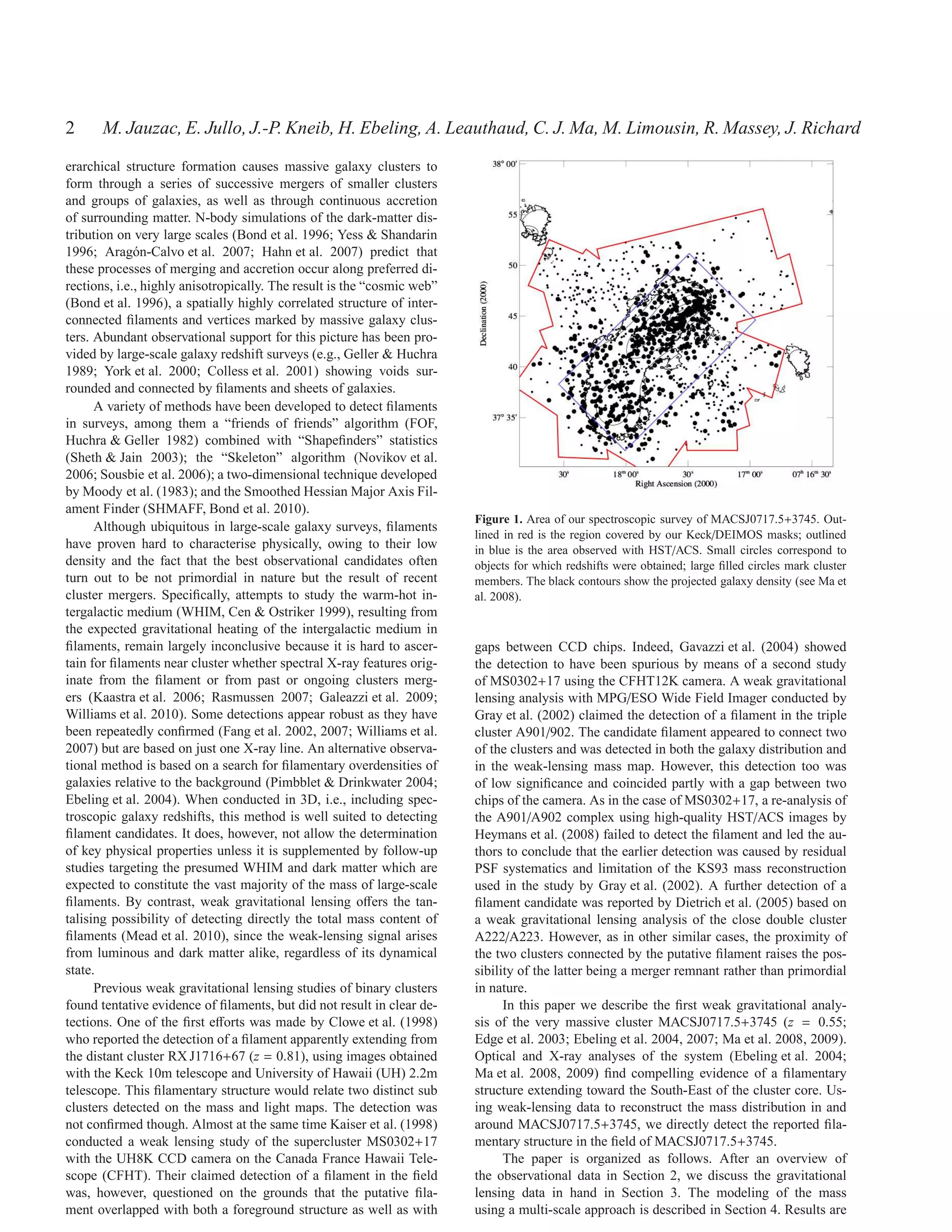
6. 6 M. Jauzac, E. Jullo, J.-P. Kneib, H. Ebeling, A. Leauthaud, C. J. Ma, M. Limousin, R. Massey, J. Richard
data causes the Subaru catalogue to be confusion limited and makes the lens-source system. The convergence κ is defined as the dimen-
matching galaxies between the two catalogues difficult, especially sionless surface mass density of the lens:
near the cluster core. As a result, we can assign a redshift to only 1 2 Σ(DOL θ)
∼ 15% of the galaxies in the HST/ACS galaxy catalogue. κ(θ) = ∇ ϕ(θ) = , (1)
2 Σcrit
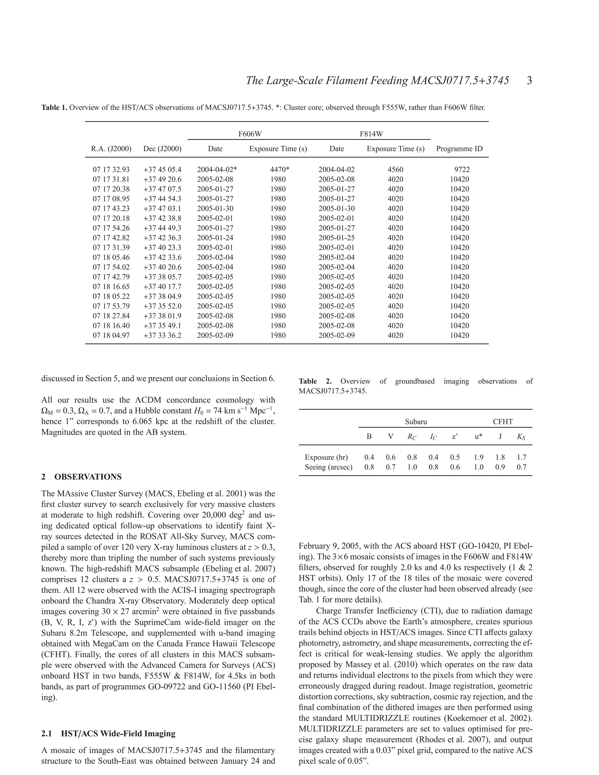
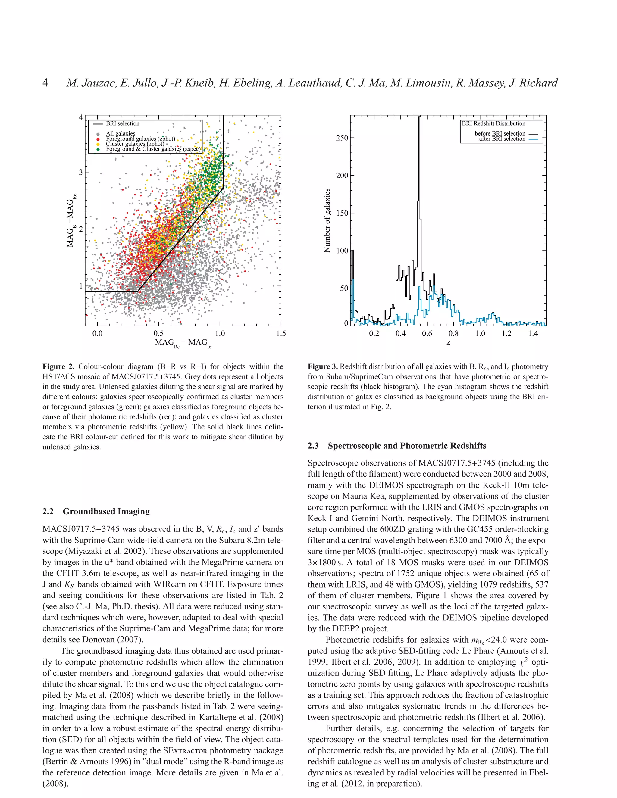
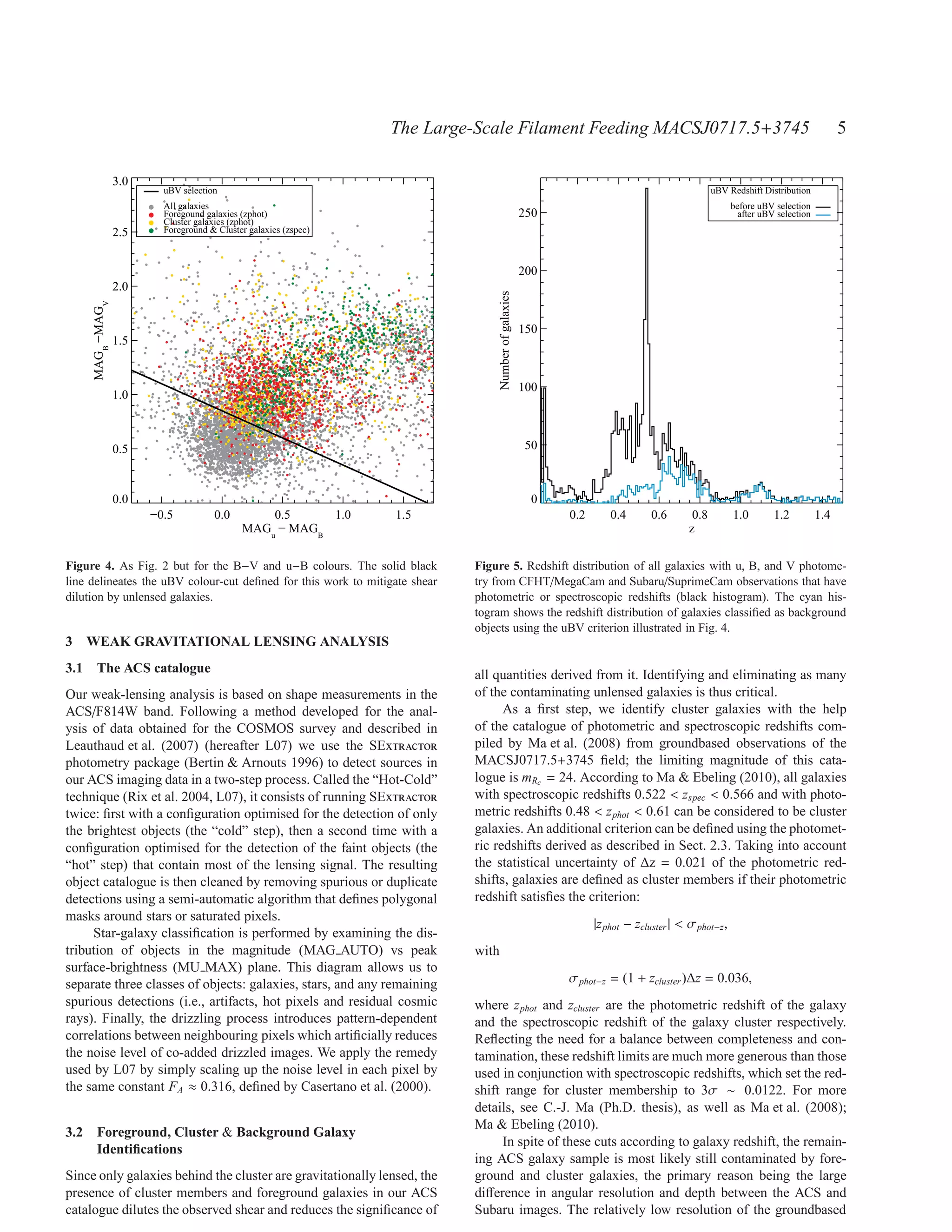
For galaxies without redshifts, we use colour-colour diagrams
(B−R vs R−I, Fig. 2, and B−V vs u−B, Fig. 4) to identify fore- where θ is the angular position of the background galaxy, ϕ is the
ground and cluster members. Using galaxies with spectroscopic or deflection potential, Σ(DOL θ) is the physical surface mass density
photometric redshifts from the full photometric Subaru catalogue of the lens, and Σcrit is the critical surface mass density defined as
with a magnitude limit of mRc = 25, we identify regions marked c2 DOS
dominated by unlensed galaxies (foreground galaxies and cluster Σcrit = .
4πGDOL DLS
members). In the BRI plane we find B−R < 2.6 (R−I) + 0.05;
(R−I) > 1.03; or (B−R) < 0.9 to best isolate unlensed galaxies; in Here, DOL , DOS , and DLS represent the angular distances from the
the UBV plane the most efficient criterion is B−V < −0.5 (u−B) + observer to the lens, from the observer to the source, and from the
0.85. lens to the source, respectively.
Figures 3 and 5 show the galaxy redshift distributions before Considering the shear γ as a complex number, we define
and after the colour-colour cuts (BRI or uBV) are applied. The re-
γ = γ1 + iγ2 ,
sults of either kind of filtering are similar. The uBV selection is
more efficient at removing cluster members and foreground galax- where γ1 = |γ| cos 2φ and γ2 = |γ| sin 2φ are the two components of
ies at z 0.6 (20% remain compared to 30% for the BRI criterion) the shear, γ, defined previously, and φ is the orientation angle. With
but also erroneously eliminates part of the background galaxy pop- this definition, the shear is defined in terms of the derivatives of the
ulation. Comparing the convergence maps for both colour-colour deflection potential as :
selection schemes, we find the uBV selection to yield a better de-
1
tection of structures in the area surrounding the cluster, indicating γ1 = (ϕ11 − ϕ22 ),
that suppressing contamination by unlensed galaxies is more im- 2
portant than a moderate loss of background galaxies from our final γ2 = ϕ12 = ϕ21 ,
catalogue (see Sect. 5 for more details).
Since the redshift distribution of the background population with
peaks at 0.61 < z < 0.70 (cyan curve in Fig. 5) we assign, in the ∂2
mass modelling phase, a redshift z = 0.65 to background galaxies ϕi j = ϕ(θ), i, j ∈ (1, 2).
∂θi ∂θ j
without redshift.
Following Kaiser & Squires (1993), the complex shear is re-
lated to the convergence by:
3.3 Shape measurements of Galaxies & Lensing Cuts
1
κ(θ) = − d2 θ′ Re[D(θ − θ′ )γ∗ (θ′ )].
3.3.1 Theoretical Weak Gravitational Lensing Background π
The shear signal contained in the shapes of lensed background Here D(θ) is the complex kernel, defined as
galaxies is induced by a given foreground mass distribution. In the 2 2
θ1 − θ2 + 2iθ1 θ2
weak-lensing regime this shear is observed as a statistical deforma- D(θ) = ,
tion of background sources. The observed shape of a source galaxy, |θ|4
ε, is directly related to the lensing-induced shear, γ, according to and Re(x) defines the real part of the complex number x. The aster-
the relation : isk denotes complex conjugation. The last equation shows that the
surface mass density κ(θ) of the lens can be reconstructed straight-
ε = εintrinsic + εlensing ,
forwardly if the shear γ(θ) caused by the deflector can be measured
where εintrinsic is the intrinsic shape of the source galaxy (which locally as a function of the angular position θ.
would be observed in the absence of gravitational lensing), and
γ
εlensing = . 3.3.2 The RRG method
1−κ
Here κ is the convergence. In the weak-lensing regime, κ ≪ 1, To measure the shape of galaxies we use the RRG method
which reduces the relation between the intrinsic and the observed (Rhodes et al. 2000) and the pipeline developed by L07. Having
shape of a source galaxy to been developed for the analysis of data obtained from space, the
RRG method is ideally suited for use with a small, diffraction-
ε = εintrinsic + γ.
limited PSF as it decreases the noise on the shear estimators by
Assuming galaxies are randomly oriented on the sky, the ellipticity correcting each moment of the PSF linearly, and only dividing them
of galaxies is an unbiased estimator of the shear, down to a limit at the very end to compute an ellipticity.
referred to as “intrinsic shape noise”, σintrinsic (for more details see The ACS PSF is not as stable as one might expect from a
L07; Leauthaud et al. 2010, hereafter L10). Unavoidable errors in space-based camera. Rhodes et al. (2007) showed that both the size
the galaxy shape measurement are accounted for by adding them in and the ellipticity pattern of the PSF varies considerably on time
quadrature to the“intrinsic shape noise”: scales of weeks due to telescope ’breathing’. The thermal expan-
sion and contraction of the telescope alter the distance between the
σ2 = σ2
γ
2
measurement + σintrinsic .
primary and the secondary mirrors, inducing a deviation of the ef-
The shear signal induced on a background source by a given fective focus and thus from the nominal PSF which becomes larger
foreground mass distribution will depend on the configuration of and more elliptical. Using version 6.3 of the TinyTim ray-tracing

7. The Large-Scale Filament Feeding MACSJ0717.5+3745 7
program, Rhodes et al. (2007) created a grid of simulated PSF im- In order to optimize the signal-to-noise ratio, we introduce an
ages at varying focus offsets. By comparing the ellipticity of ∼ inverse-variance weighting scheme following L10:
20 stars in each image to these models, Rhodes et al. (2007) were
able to determine the effective focus of the images. Tests of this 1
wγ =
˜ .
algorithm on ACS/WFC images of dense stellar fields confirmed σ2
γ
˜
that the best-fit effective focus can be repeatedly determined from
a random sample of 10 stars brighter than mF814W = 23 with an Hence faint small galaxies which have large measurement errors
rms error of 1µm. Once images have been grouped by their effec- are down-weighted with respect to sources that have well measured
tive focus position, the few stars in each images can be combined shapes.
into one large catalog. PSF parameters are then interpolated using
a polynomial fit in the usual weak-lensing fashion (Massey et al.
2002). More details on the PSF modelling scheme are given in
Rhodes et al. (2007). 3.3.4 Lensing Cuts
The RRG method returns three parameters: d, a measure of the
galaxy size, and, the ellipticity represented by the vector e = (e1 , e2 ) The last step in constructing the weak-lensing catalogue for the
defined as follows: MACSJ0717.5+3745 field consists of applying lensing cuts, i.e.,
to exclude galaxies whose shape parameters are ill-determined and
a2 − b2 will increase the noise in the shear measurement more than they add
e =
a2 + b2 to the shear signal. However, in doing so, we need to take care not
e1 = e cos(2φ) to introduce any biases. We use three galaxy properties to establish
e2 = e sin(2φ), the following selection criteria:
where a and b are the half-major and half-minor axis of the back- • Their estimated detection significance:
ground galaxy, respectively, and φ is the orientation angle of the
ellipse defined previously. The ellipticity e is then calibrated by a S FLUX AUT O
= > 4.5;
factor called shear polarizability, G, to obtain the shear estimator γ:
˜ N FLUXERR AUT O
e where FLUX AUTO and FLUXERR AUTO are parameters re-
γ=C
˜ . (2)
G turned by SExtractor;
The shear susceptibility factor G is measured from moments of the • Their total ellipticity:
global distribution of e and other shape parameters of higher or-
der (see Rhodes et al. 2000). The Shear TEsting Program (STEP; e= e2 + e2 < 1;
1 2
Massey et al. 2007) for COSMOS images showed that G is not con-
stant but varies as a function of redshift and S/N. To determine G • Their size as defined by the RRG d parameter:
for our galaxy sample we use the same definition as the one used
for the COSMOS weak-lensing catalogue (see L07): d > 0.13′′ .
S /N − 17
G = 1.125 + 0.04 arctan . The requirement that the galaxy ellipticity be less than unity
4
may appear trivial and superfluous. In practice it is meaningful
Finally, C, in Eq. 2 is the calibration factor. It was determined though since the RRG method allows measured ellipticity values
using a set of simulated images similar to those used by STEP to be greater than 1 because of noise, although ellipticity is by def-
(Heymans et al. 2006; Massey et al. 2006) for COSMOS images, inition restricted to e 1. Because Lenstool prevents ellipticities
and is given by C = (0.86−0.05 )−1 (for more details see L07).
+0.07
to be larger than 1, we removed the 251 objects with an ellipticity
greater than unity from the RRG catalogue (2% of the catalogue).
Serving a similar purpose, the restriction in the RRG size parameter
3.3.3 Error of the Shear Estimator d aims to eliminate sources with uncertain shapes. PSF corrections
become increasingly significant as the size of a galaxy approaches
As explained in Sect. 3.3.1, the uncertainty in our shear estimator that of the PSF, making the intrinsic shape of a galaxy difficult to
is a combination of intrinsic shape noise and shape measurement measure.
error: Our final weak-lensing catalogue is composed of 10170 back-
σ2 = σ2 2 ground galaxies, corresponding to a density of ∼ 52 galaxies
γ
˜ intrinsic + σmeasurement ,
arcmin−2 . In addition to applying the aforementioned cuts, and in
2
where σγ is referred to as shape noise. The shape measurement
˜ order to ensure an unbiased mass reconstruction in the weak lens-
error is determined for each galaxy as a function of size and mag- ing regime only, we also remove all background galaxies located
nitude. Applying the method implemented in the PHOTO pipeline in the multiple-image (strong-lensing) region defined by an ellipse
(Lupton et al. 2001) to analyze data from the Sloan Digital Sky Sur- aligned with the cluster elongation and with a semi-major axis of
vey, we assume that the optical moments of each object are the 55”, a semi-minor axis of 33”. From the resulting mass-map pre-
same as the moments computed for a best-fit Gaussian. Since the sented in Sect. 5, we a-posteriori derived a convergence histogram
ellipticity components (which are uncorrelated) are derived from of the pixels outside this region, and found that 90% of them are
the moments, the variances of the ellipticity components can be smaller than κ = 0.1, with a mean value of κ = 0.03. The shear
obtained by linearly propagating the covariance matrix of the mo- and convergence are so weak because the ratio DLS /DOS = 0.14
ments. The value of the intrinsic shape noise, σintrinsic , is taken to be for background galaxies at redshift zmed = 0.65 and the cluster at
0.27 (for more details see L07, L10). z = 0.54 (see Sect. 4).

8. 8 M. Jauzac, E. Jullo, J.-P. Kneib, H. Ebeling, A. Leauthaud, C. J. Ma, M. Limousin, R. Massey, J. Richard
4 MASS DISTRIBUTION
The mass modelling for the entire MACSJ0717.5+3745 field is
performed using the LENSTOOL1 (Jullo et al. 2007) software, us-
ing the adaptive-grid technique developed by Jullo & Kneib (2009)
and modified by us for weak-lensing mass measurements. Because
LENSTOOL implements a Bayesian sampler, it provides many
mass maps fitting the data that can be used to obtain a mean mass
map and to determine its error.
4.1 Multi-Scale Grid Method
We start with the method proposed by Jullo & Kneib (2009) to
model the cluster mass distribution using gravitational lensing. This Figure 6. Distribution of grid nodes and galaxy-scale potentials, superim-
recipe uses a multi-scale grid of Radial Basis Functions (RBFs) posed on the K-band light map of MACSJ0717.5+3745. Cyan crosses rep-
with physically motivated profiles and lensing properties. With a resent the location of 468 RBFs at the nodes of the multi-scale grid; magenta
minimal number of parameters, the grid of RBFs of different sizes circles represent galaxy-scale potentials used to describe the contribution of
provides higher resolution and sharper contrast in regions of higher individual cluster members. The white dashed line defines the HST/ACS
density where the number of constraints is generally higher. It is field of view. The white cross marks the cluster centre at 07:17:30.025,
+37:45:18.58 (R.A., Dec).
well suited to describe irregular mass distributions like the one in-
vestigated here.
The initial multi-scale grid is created from a smoothed map
Jullo & Kneib (2009) found to yield an optimal compromise be-
of the cluster K-band light and is recursively refined in the densest
tween model flexibility and overfitting. We then adapt the technique
regions. In the case of MACSJ0717.5+3745, this method is fully
proposed by Diego et al. (2007) to our multiscale grid model to fit
adaptive as we want to sample a wide range of masses, from the
the weak-lensing data (κ ≪ 1). Assuming a set of M images and a
cluster core to the far edge of the HST/ACS field where the fil- i
model comprised of N RBFs, the relation between the weights σ2 0
amentary structure is least dense. Initially, the field of interest is
and the 2M components of the shear is given by
limited to a hexagon, centred on the cluster core and split into six
equilateral triangles (see Fig. 1 in Jullo & Kneib 2009). This initial
  (1,1)
∆(1,N)
 1
···

grid is subsequently refined by applying a splitting criterion that is  γ1
   ∆1
  1 

  . .

based on the surface density of the light map. Hence, a triangle will  .


 .  
 
  . .. .



.
  
. .   σ2 1
 .   
 
  
be split into four smaller triangles if it contains a single pixel that
   (M,1)

 M
 γ
   (M,N)  0
 

  ∆ ··· ∆1

 1  
  1  .
 


exceeds a predefined light-surface-density threshold.  .


  =  (1,1)
 
  
 .


∆(1,N)
 1
 γ 
  ∆ ···
   
 

Once the adaptive grid is set up, RBFs described by Trun-
 2   2 2  


 .  
    2N

 σ


. .
 
cated Isothermal Mass Distributions (TIMD), circular versions

 .  
  . .. .

 0
.

 .  
. .
  


  
 
 



of truncated Pseudo Isothermal Elliptical Mass Distributions  M   (1,M) (M,N)

γ2

∆2 ··· ∆2
(PIEMD) (see, e.g., Kassiola & Kovner 1993; Kneib et al. 1996;
Limousin et al. 2005; El´asd´ ttir et al. 2007) are placed at the grid
ı o with
node locations. The analytical expression of the TIMD mass sur- DiLS (i, j)
face density is given by ∆(i, j) =
1 γ ,
DiOS 1
2
Σ(R) = σ0 f (R, rcore , rcut )
DiLS (i, j)
with ∆(i, j) =
2 γ ,
  DiOS 2
 
1 rcut 1 1
 
f (R, rcore , rcut ) =




 −


.

 where
2G rcut − rcore
 
rcore + R2
2
 
 2
rcut +R 2
 1
γ1 j) =
(i,

(∂11 Φ j (Ri j ) − ∂22 Φi (Ri j )),
2
Hence, f defines the profile, and σ2 defines the weight of the
0
RBF. This profile is characterized by two changes in slope at ra- γ2 j) = ∂12 Φ j (Ri j ) = ∂21 Φ j (Ri j ),
(i,
dius values of rcore and rcut . Within rcore , the surface density is ap-
proximately constant, between rcore and rcut , it is isothermal (i.e., and
Σ ∝ r−1 ), and beyond rcut it falls as Σ ∝ r−3 . This profile is physi- Ri j = |θi − θ j |.
cally motivated and meets the three important criteria of a) featur-
ing a finite total mass, b) featuring a finite central density, and c) In the above, DiLS and DiOS are the angular distances from the
being capable of describing extended flat regions, in particular in RBF j to the background source i and from the observer to the
the centre of clusters. background source i, respectively, and Φ is the projected gravita-
The RBFs’ rcore value is set to the size of the smallest nearby tional potential. γk=1,2 are the two components of the shear, ∆(i, j)
k=1,2
triangle, and their rcut parameter is set to 3rcore , a scaling that j
is the value of the RBF normalized with σ2 = 1, centered on the
0
grid node located at θ j , and computed at a radius R = |θi − θ j |.
The contribution of this RBF to the predicted shear at location θi is
j
1 LENSTOOL is available online: http://lamwws.oamp.fr/lenstool given by the product ∆(i, j) σ2 (see Eq. 1). More details about this
k=1,2 0

9. The Large-Scale Filament Feeding MACSJ0717.5+3745 9
method will be provided in a forthcoming paper (Jullo et al. 2012,
in preparation).
Figure 6 shows the distribution of the 468 RBFs superimposed
on the light map used to define the multi-scale grid. The smallest
RBF has a rcore = 26′′ . Note that although Lenstool can perform
strong lensing, and reduced-shear optimization, here the proposed
formalism assumes weak-shear with κ ≪ 1. To get an unbiased es-
timator, we remove the background galaxies near the cluster core
from the catalogue, but we keep RBFs in this region as we found it
improves the mass reconstruction. In order to check our weak-shear
assumption, we multiply the resulting convergence map by the fac-
tor 1 − κ, and find this minor correction only represents about 5% at
300 kpc and less than 1% at 500 kpc. It confirms that working with
a weak-shear assumption in this case is not biasing our results. On Figure 7. Contours of the convergence κ in the MACS0717.5+3745 field
Fig. 8, the black dashed curve corresponds to the corrected weak- obtained using the inversion method described by Seitz & Schneider (1995),
shear optimization, while the black curve represents the weak-shear overlaid on the K-band light map. Magenta contours represent the 1, 2 and
optimization profile. Both shows a really good agreement with the 3σ contours. Cyan crosses mark the position of two galaxy groups (see text
strong-lensing results (magenta curve). for details). The white cross marks again the cluster centre (cf. Fig. 6).
4.3 Mass Modeling
4.2 Cluster Member Galaxies
The mass reconstruction is conducted using LENSTOOL which
Our catalogue of cluster members is compiled from the photomet- implements an optimisation method based on a Bayesian Markov
ric catalogue of Ma et al. (2008). Within the HST/ACS study area Chain Monte Carlo (MCMC) approach (Jullo et al. 2007). We
we identify as cluster members 1244 galaxies with spectroscopic chose this approach because we want to propagate as transparently
and/or photometric redshifts within the redshift ranges defined in as possible errors on the ellipticity into errors on the filament mass
Sect. 3.2. We use these galaxies’ KS -band luminosities as mass es- measurement. This method provides two levels of inference: pa-
timators (see below for details). rameter space exploration and model comparison, by means of the
All cluster members are included in the lens model in the form posterior Probability Density Function (PDF) and the Bayesian ev-
of truncated PIEMD potentials (see Sect. 4.1) with characteristic idence, respectively.
properties scaled according to their K-band luminosity: All of these quantities are related by the Bayes Theorem:
1/2 Pr(D|θ, M)Pr(θ|M)
∗ L Pr(θ|D, M) ∝ ,
rcore = rcore , Pr(D|M)
L∗
where Pr(θ|D, M) is the posterior PDF, Pr(D|θ, M) is the likelihood
L 1/2 of a realisation yielding the observed data D given the parameters
∗
rcut = rcut , θ of the model M, and, Pr(θ|M) is the prior PDF for the parame-
L∗
ters. Pr(D|M) is the probability of obtaining the observed data D
and, given the assumed model M, also called the Bayesian evidence. It
1/4 measures the complexity of the model. The posterior PDF will be
L
σ0 = σ∗
0 . the highest for the set of parameters θ that yields the best fit and
L∗ is consistent with the prior PDF. Jullo et al. (2007) implemented an
These scaling relations are found to well describe early- annealed Markov Chain to converge progressively from the prior
type cluster galaxies (e.g. Wuyts et al. 2004; Fritz et al. 2005) un- PDF to the posterior PDF.
der the assumptions of mass tracing light and the validity of the For the weak-lensing mass mapping, we implement an addi-
Faber & Jackson (1976) relation. Since the mass, M, is propor- tional level of complexity based on the Gibbs sampling technique
tional to σ2 rcut , the above relations ensure M ∝ L, assuming that
0
(see Massive Inference in the Bayesys manual, Skilling 1998). Ba-
the mass-to-light ratio is constant for all cluster members. sically, only the posterior distribution of the most relevant RBFs is
To find suitable values of rcore , rcut , and σ∗ we take advantage
∗ ∗ explored. The number of RBFs to explore is an additional free pa-
0
of the results of the strong-lensing analysis of MACSJ0717.5+3745 rameter with a Poisson prior. Exploring possible values of this prior
recently conducted by Limousin et al. (2012). Their mass model of in simulations, we find that the input mass is well recovered when
the cluster also included cluster members, using the scaling rela- the mean of this prior is set to 2% of the total number of RBFs in
i
tions defined above (see also Limousin et al. 2007). For a given L∗ the model. The weights of the RBFs, σ2 , are decomposed into the
0
luminosity, given by m∗ = 19.16, the mean apparent magnitude of product of a quantum element of weight, q, common to all RBF,
a cluster member in K-band, Limousin et al. (2012) set all geomet- and a multiplicative factor ζ i . In order to have positive masses, we
rical galaxy parameters (centre, ellipticity, position angle) to the make ζ follow a Poisson prior (case MassInf=1), and q to follow
∗
values measured with SExtractor, fixed rcore at 0.3 kpc, and then the prior distribution π(q) = q−2 q exp−q/q0 , and we fix the initial
0
∗ ∗ i
searched for the values of σ0 and rcut that yield the best fit. We here guess q0 = 10 km2 /s2 . The final distribution of σ2 is well approxi-
0
∗ ∗
use the same best-fit values, rcut = 60 kpc and σ0 = 163 kpc/s, to mated by a distribution π(q) with q0 = 12 km2 /s2 , and, we find that
define the potentials of the cluster members. Hence, all parameters 16.8 ± 4.8 RBFs are necessary on average to reconstruct the mass
describing cluster members are fixed in our model; their positions distribution given our data, i.e. about 3.5% of the total number of
are marked by the magenta circles in Fig. 6. RBFs in the model. This new algorithm is fast, as it can deliver a

10. 10 M. Jauzac, E. Jullo, J.-P. Kneib, H. Ebeling, A. Leauthaud, C. J. Ma, M. Limousin, R. Massey, J. Richard
Figure 9. Mass distribution in the core of MACSJ0717.5+3745. Cyan con-
tours represent the mass distribution inferred in the strong-lensing study by
Limousin et al. (2012); white contours show the mass distribution obtained
by our weak-lensing analysis; and magenta contours represent the distribu-
tion of the cluster K-band light. The orange cross marks the cluster center
adopted in the analysis (cf. Fig. 6).
mic Bayesian evidence is then given by
Figure 8. Density profiles within the core of MACSJ0717.5+3749. The ma-
genta curve represents strong-lensing results from Limousin et al. (2012); 1
1
the black curve shows the profile derived from our weak-lensing analysis; log(E) = − χ2 λ dλ
2 0
the black dashed curve shows the weak-lensing profile corrected from the
weak-shear approximation where the average is computed over a set of 10 MCMC realizations
at any given iteration step λi , and the integration is performed over
. The grey area marks the region within which multiple images are observed.
all iterations λi from the initial model (λ = 0) to the best-fit result
(λ = 1). An increment in dλ depends on the variance between the
10 likelihoods computed at a given iteration, and a convergence
mass map in 20 minutes for about 10,000 galaxies and 468 RBFs rate that we set equal to 0.1 (see Bayesys manual for details). The
— the previous algorithm used in Jullo & Kneib (2009) was taking increment gets larger as the algorithm converges towards 1.
more than 4 weeks to converge. The new algorithm has been tested
in parallel on five processors clocked at 2 GHz.
We define the likelihood function as (see e.g. Schneider et al. 5 RESULTS
(2000):
5.1 Kappa Map : Standard mass reconstruction
1 χ2
Pr(D|θ) = exp (− ), We test our catalogue of background galaxies by mapping the con-
ZL 2
vergence κ in the MACSJ0717.5+3745 field. We use the method
where D is the vector of ellipticity component values, and θ is a described in Sect. 3.3.1, which is based on the inversion equa-
vector of the free parameters σ2 . χ2 is the usual goodness-of-fit
i tion found by Kaiser & Squires (1993) and developed further by
statistic: Seitz & Schneider (1995). It shows that the best density recon-
M 2 structions are obtained when the smoothing scale is adapted to the
(˜ j,i − 2γ j,i (θi ))2
γ
χ2 = . (3) strength of the signal. We find a smoothing scale of 3 arcmin to
i=1 j=1
σ2
γ˜ provide a good compromise between signal-to-noise considerations
and map resolution. We estimate the noise directly from the mea-
The 2M intrinsic ellipticity components (M is the number of back-
sured errors, σmeasurement , averaged within the grid cells.
ground sources), are defined as follows:
The resulting κ-map is shown in Fig. 7, overlaid on a smoothed
εintrinsic, j = γ j (θ j ) − 2γ j (θ j )
˜ (4) image of the K-band light from cluster galaxies. We identify two
substructures south-east of the cluster core whose locations match
and, are assumed to have been drawn from a Gaussian distribution the extent of the filamentary structure seen in the galaxy distribu-
with variance defined in Sect. 3.3.1 : tion. The first of these, near the cluster core, coincides with the
beginning of the optical filament; the second falls close to the ap-
σ2 = σ2
γ
˜
2
intrinsic + σmeasure .
parent end of the filament close to the edge of our study area. A
The normalization factor is given by simple inversion technique thus already yields a 2 sigma detections
of parts of the filament.
M
√ The Chandra observation of MACS0717.5+3745 shows X-
ZL = 2π σγi .
˜ ray detections of two satellite groups of galaxies embedded in the
i=1
filament (private communication H. Ebeling, see also Fig. 1 of
Note the factor of 2 in Eqn. 3 and 4 because of the particular Ma et al. 2009, and Fig. 10 of this paper). Their X-ray coordinates
definition of the ellipticity in RRG (see Sect. 3.3.2). The logarith- (R.A., Dec, J2000) are : i) 07:17:53.618, +37:42:10.46, and, ii)

11. The Large-Scale Filament Feeding MACSJ0717.5+3745 11
Figure 10. Mass map from our weak-gravitational lensing analysis overlaid on the light map of the mosaic. The two sets of contours show the X-ray surface
brightness (cyan), and weak-lensing mass (white). The bold white contour corresponds to a density of 1.84 × 108 h74 M⊙ .kpc−2 . The orange cross marks the
location of the fiducial cluster centre, and the two blue crosses show the positions of the two X-ray detected satellite groups mentioned in Sect. 5.1. The dashed
cyan lines delineates the edges of the Chandra/ACIS-I field of view. The yellow box, finally, marks the cluster core region shown in Fig. 9. The magenta line
emphasises the extent and direction of the large-scale filament.
07:18:19.074, +37:41:13.14 (cyan crosses in Fig. 7). The first of the cluster centre because it marks the barycenter of the Einstein
these, close to the filament-cluster interface, is detected by the in- ring measured by Meneghetti et al. (2011). Another SL analysis of
version technique, but not the second. Conversely, the peak in the MACSJ0717.5+3745 was performed by Zitrin et al. (2009) who re-
convergence map in the southeastern corner of our study area is not port a mass of MSL (R < 350 kpc) = (7.0 ± 0.5) 1014 h−1 M⊙ .
74
detected in X-rays. Figure 8 compares the mass density profiles derived from the
SL analysis (magenta line) and from our WL analysis (black line);
note the very good agreement. The WL density profile has been cut
5.2 Mass Map : Iterative mass reconstruction up to ∼300 kpc as this region corresponds to the multiple-image
regime, therefore does not contain any WL constraints.
The primary goal of this paper is the detection of the large-scale
In Fig. 8, the SL density profile is extrapolated beyond the
filament with weak-lensing techniques and the characterisation of
multiple-image region (the cluster core), while the WL density
its mass content. To calibrate the mass map of the entire structure
profile is extrapolated into the multiple-image region. The WL
(i.e., filament + cluster core) and overcome the mass-sheet degen-
mass thus obtained for the cluster core is MWL (R < 500 kpc) =
eracy, we compare the weak-lensing mass obtained for the cluster
(1.04 ± 0.08) 1015 h−1 M⊙ in excellent agreement with the value
74
core with the technique described in Sect. 4, with the strong lensing
measured by Limousin et al. (2012). We also measure MWL (R <
(SL) results from Limousin et al. (2012).
350 kpc) = (5.10 ± 0.54) 1014 h−1 M⊙ , in slight disagreement with
74
the result reported by Zitrin et al. (2009). But the excellent agree-
ment at larger radii between strong- and weak-lensing results with-
5.2.1 Cluster Core
out any adjustments validates our redshift distribution for the back-
Limousin et al. (2012) inferred a parametric mass model for the ground sources, and our new reconstruction method.
core of MACSJ0717.5+3745 using strong-lensing (SL) constraints, Figure 9 compares the mass contours from the two different
specifically 15 multiple-image systems identified from multi-color gravitational-lensing analyses for the core of MACSJ0717.5+3745
data within a single HST/ACS tile. Spectroscopic follow up of and illustrates the remarkable agreement between these totally in-
the lensed features allowed the determination of a well calibrated dependent measurements. Our WL analysis requires a bi-modal
mass model. The cyan contours in Fig. 9 show the mass dis- mass concentration which coincides with the two main concentra-
tribution obtained from their analysis. Four mass components, tions inferred by the SL analysis of Limousin et al. (2012).
associated with the main light components, are needed to sat-
isfy the observational constraints. The cluster mass reported by
Limousin et al. (2012) for the region covered by a single ACS
5.2.2 Detection of a filamentary structure
field-of-view is MSL (R < 500 kpc) = (1.06 ± 0.03) 1015 h−1 M⊙
74
where the cluster centre is taken to be at the position quoted be- Figure 10 shows the mass map obtained for the whole HST/ACS
fore (07:17:30.025 +37:45:18.58). This position was adopted as mosaic using the modeling and optimization method described

12. 12 M. Jauzac, E. Jullo, J.-P. Kneib, H. Ebeling, A. Leauthaud, C. J. Ma, M. Limousin, R. Massey, J. Richard
in Sect. 4. Also shown are the X-ray surface brightness as ob-
served with Chandra/ACIS-I, and the cluster K-band light. A fil- Density Profiles (outer regions)
amentary structure extending from the south-eastern edge of the whole HST/ACS field
Filament inner part
cluster core to the south-eastern edge of the ACS mosaic area is Cluster
109 Σ(R) ∝ R-1
clearly visible in all three datasets. The projected length of the fil- Σ(R) ∝ R-2
ament is measured as 4.5 h−1 Mpc, and the mean density in the
74
region of the filament is found to be (2.92 ± 0.66) × 108 h74 M⊙
Surface Mass Density (h74 MO kpc-2)
kpc−2 . The mass concentration detected to the South-East of the
•
cluster core corresponds to a low-mass structure comparable to
a galaxy group and indeed coincides with a poor satellite cluster
of MACSJ0717.5+3745 that has been independently identified as
an overdensity of galaxies and as a diffuse peak in the X-ray sur-
face brightness. The second, more compact, X-ray emitting galaxy
group (almost due East of the cluster core and outside the filament)
is also detected. 108
To assess the validity of this filament detection, we test the ro-
bustness of our multi-scale grid optimization method. As a first step
we create a uniform grid with a RBF of size rcore = 21′′ and 3169
potentials. We found that using this uniform grid added noise in lo-
cations where no structures were detected neither in the optical, nor
1000
in the mass map produced with the multi-scale grid. The Bayesian Radius (h74-1 kpc)
evidence obtained for the uniform grid (pixel size of rcore = 21′′ )
is log(E) = −6589, compared to log(E) = −6586 for the multi- Figure 11. Profile of the mass surface density of the cluster/filament com-
scale grid (pixel size of rcore = 26′′ ). The small difference between plex as a function of distance from the cluster core. The three curves show
these two values demonstrates that the reduced number of RBFs in the mass surface density measured in our weak-lensing analysis across the
our multi-scale grid does not compromise the measurement. This entire field (black), for the cluster without the filament (cyan), and for the
is further confirmed by a test using a low-resolution uniform grid inner part of the filament (orange). The two green lines represent two dif-
with a pixel size of rcore = 43′′ comprising 817 RBFs, for which we ferent slopes: R−1 and R−2 . See text for details.
found a Bayesian evidence of log(E) = −6582. All 3 grids equiv-
alently reproduce the data. Our multi-scale grid model provides an
intermediate resolution map. inhabiting the nodes of the cosmic web. Taking advantage of the
Having established that the use of an adaptive grid has no opportunity provided by this special target, Ma et al. (2008) pur-
detrimental effect on the Bayesian evidence, the second test con- sued a wide-field spectroscopic analysis of the galaxy population
sisted in increasing the resolution of the multi-scale grid to a pixel of both the cluster and the filament. Along the filament, they found
size of rcore = 13′′ , resulting in 2058 potentials. We found that a significant offset in the average redshift of galaxies, correspond-
the noise increased with the resolution, whereas all real mass con- ing to ∼ 630 km s−1 in velocity, as well as a decrease in velocity
centrations maintained their size. The Bayesian evidence obtained dispersion from the core of the cluster to the end of the filament.
with this high-resolution multi-scale grid is log(E) = −6608. A Ma & Ebeling (2010) studied the morphology of cluster members
WL mass reconstruction with the high-resolution multi-scale grid across a 100 h−2 Mpc2 area to investigate the effect of cluster envi-
74
recovers the density profile obtained with the multi-scale grid us- ronment on star formation using HST/ACS data. They explored the
ing rcore = 26′′ pixels. However, in view of the large difference relation between galaxy color and density. They showed that the
between these two evidence values, it is clear that such an increase 1-D density profile of MACSJ0717.5+3745 cluster members fol-
in resolution is not required by the data. lowed the filament from the core to beyond the virial radius falling,
then slightly rising and flattening at ∼ 2h−1 Mpc.
74
To physically characterise the large-scale filament, we 1) anal-
yse its density profile (Fig. 11); 2) study the variation of its diame-
6 PROPERTIES OF THE FILAMENT ter as a function of distance to the cluster core (Fig. 12); 3) derive a
schematic picture of its geometry and orientation along the line of
In this Section, we first summarise briefly the results of previous
sight (Figs. 13 & 14); and 4) attempt to measure the mass in stars
studies of the MACSJ0717.5+3745 filament, and then discuss the
within the entire structure (Fig. 15).
filament’s properties as derived from our weak-lensing analysis.
The detection of a filamentary structure in the field of the clus-
ter MACSJ0717.5+3745 was first reported by Ebeling et al. (2004),
6.1 Density Profiles
who discovered a pronounced overdensity of galaxies with V−R
colours close to the cluster red sequence, extending over ∼ 4h−1 74 Figure 11 shows the density profile across the entire study area as
Mpc at the cluster redshift. Extensive spectroscopic follow-up of a function of distance from the cluster centre as defined and shown
over 300 of these galaxies in a region covering both the cluster and in Figs. 6, 7, 9, and 10. Also shown are the profiles of the filament
the filament confirmed that the entire structure is located at the clus- only (obtained by only considering the WL mass along the magenta
ter redshift, z = 0.545. This direct detection of an extended large- line and within the bold white contour in Fig. 10), and of the cluster.
scale filament connected to a massive, distant cluster lent strong The cluster density profile is cut at 2 h−1 Mpc from the cluster core
74
support to predictions from theoretical models and numerical sim- as further, the ACS field is dominated by the filament.
ulations of structure formation in a hierarchical scenario, according As is apparent from both Figs. 10 and 11, the filament con-
to which large-scale filaments funnel matter toward galaxy clusters nects to the cluster at a distance of about 1.5h−1 Mpc from the clus-
74

13. The Large-Scale Filament Feeding MACSJ0717.5+3745 13
Figure 12. Diameter of the filamentary structure as a function of distance
from the cluster centre. The regime of the cluster proper and the segment
containing the embedded X-ray bright group of galaxies (blue cross in
Fig. 10) are marked. The density threshold used to define the filamentary
structure is 1.84 × 108 h74 M⊙ .kpc−2 .
ter core, causing the density profile to flatten from this distance
outward. The mean density in this region is (2.92 ± 0.66) × 108 h74
M⊙ kpc−2 . The embedded galaxy group detected also in the clus-
Figure 13. Schematic presentation of the geometry of the large-scale fila-
ter light and at X-ray wavelengths is responsible for the peak in the
ment along the line of sight, as deduced from radial-velocity measurements.
density profile at a distance of about 2h−1 Mpc from the cluster cen-
74 Over the first 4 Mpc (in projection) the filament’s average inclination angle
tre. The dip in the filament profile at ∼2.8 h−1 Mpc from the cluster
74 is found to be α ∼ 75. Beyond this projected distance, the filament curves
centre coincides with a dip visible also in projection in Fig. 10 (see increasingly toward the plane of the sky, eventually rendering its projected
Sect. 6.3 for more details on the 3D geometry of the large-scale mass surface density too low to be detectable. In this sketch, radial veloci-
filament). The filament clearly dominates the radial density pro- ties as observed are split into two components: peculiar velocities and Hub-
file from ∼2 h−1 Mpc from the cluster centre until the edge of the
74
ble flow, all expressed relative to the radial velocity of the cluster core.
HST/ACS field. (Adapted from Ebeling et al. 2012.)
Fitting any of these profiles with parametric models (NFW,
SIS, etc) is not meaningful in view of the complexity and obvious
non-sphericity of these structures. We note, however, that the over- Figure 12 shows the results thus obtained as a function of dis-
all density profile decreases as R−2 until about 2 h−1 Mpc, where the tance from the cluster centre. We find the filament’s diameter to de-
74
beginning of the filament causes a dramatic flattening of the den- crease with increasing distance from the cluster centre, albeit with
sity profile. For illustrative purposes, Fig. 11 shows two different mild local variations. Recognizable features are the local peak at
slopes, R−1 and R−2 . 1.85 h−1 Mpc from the cluster centre where the presence of an
74
embedded group of galaxies (marked by a blue cross in Fig. 10)
combined with a second, X-ray faint mass concentration causes the
6.2 Filament Size filament to widen to (2.79 ± 0.45) h−1 Mpc. The following narrow-
74
ing of the filament at a cluster-centric distance of about 2.8 h−1 Mpc
74
We define the region of the filament on the mass map by a den-
coincides with a dip in the filament density (cf. Sect. 6.1). Two ad-
sity threshold of 1.84 × 108 h74 M⊙ .kpc−2 which corresponds to the ditional increases in size (neither of them detected in X-rays) are
3 sigma detection contour of the lensing mass reconstruction, and observed at larger distances of approximately 3.6 and 4.7 h−1 Mpc
74
then define the central axis of the filament with respect to this con-
and can again be matched to local peaks in the filament density and
tour (magenta line in Fig. 10). Under the simplifying assumption projected WL mass density (Figs. 11 and 10, respectively).
that the filament cross-section is spherical (i.e., the filament resem-
bles a cylinder of variable radius), the filament diameter is given by
the perpendicular distance of the contour to this axis. The uncer-
6.3 3D-properties of the large-scale filament
tainty of this measurement is assessed by repeated this procedure
for every mass map produced by LENSTOOL, and adopting the In order to derive intrinsic properties of the filament from the
standard deviation of the results as the error of the filament diame- observables measured in projection, we need to know the three-
ter. dimensional orientation and geometry of the filament and, specif-

14. 14 M. Jauzac, E. Jullo, J.-P. Kneib, H. Ebeling, A. Leauthaud, C. J. Ma, M. Limousin, R. Massey, J. Richard
1000
<M∗/LK> = 0.94 ± 0.41
Σ ∼ R-1
Σ ∼ R-2
800
Stellar Mass Density (h74 MO kpc-2)
107
•
600
ρfilament / ρcrit
400
200
106
0
0 20 40 60 80 1000
α(o) Radius (h74-1 kpc)
Figure 14. Mass density of the filament in units of ρcrit as a function of the Figure 15. Density profile of the stellar component in the whole HST/ACS
orientation angle α. The red diamond highlights the density for the adopted field of MACSJ0717.5+3745. The stellar mass is obtained using the
average inclination angle of 75 deg. Arnouts et al. (2007) relation for a red galaxy population, and an Salpeter
IMF. The mean M∗ /LK ratio is equal to 0.94 ± 0.41 for our galaxy popula-
tion. The two green curves represent two different slopes: R−1 & R−2 , light
and dark green respectively.
ically, its inclination with respect to the plane of the sky. Ebeling
et al. (2012, in preparation) derive a model of the entire complex 6.4 Stellar Mass Fraction
by comparing the measured variation in the mean radial velocity To compute the stellar mass, M∗ , across our study region we use
of galaxies along the filament axis to expectations from Hubble- the relation log(M∗ /LK ) = az + b established by Arnouts et al.
flow velocities, as well as with the predictions of peculiar veloc- (2007) for quiescent (red) galaxies in the the VVDS sample
ities within filaments from numerical simulations (Colberg et al. (Le F` vre et al. 2005) and adopting a Salpeter initial mass func-
e
2005; Cuesta et al. 2008; Ceccarelli et al. 2011). A self-consistent tion (IMF). Here LK is the galaxy’s luminosity in the K band, z is
description is obtained for an average inclination angle of the fil- its redshift, and the parameters a and b are given by
ament with respect to the plane of the sky of about 75 degrees
(Fig. 13). At this steep inclination, the three-dimensional length of a = −0.18 ± 0.03 b = −0.05 ± 0.03.
the filament reaches 18 h−1 Mpc within our study region. We apply this relation to the K-band magnitudes of all cluster mem-
Using the weak-lensing mass map and the above model of the bers, defined using the redshift criteria presented in Sect. 3. The K-
3D geometry and orientation of the filament, we can constrain the band magnitude limit of our catalogue is 23.1. The resulting pro-
filament’s intrinsic density. Adopting again a cylindrical geometry jected mass density in stars is shown in Fig. 15 as a function of
and the average projected values from Figs. 11 and 12 we obtain a distance from the cluster centre. It decreases in proportion to the to-
mass density of ρfilament = (3.13 ± 0.71) × 1013 h2 M⊙ Mpc−3 , or
74 tal projected mass density depicted in Fig. 11, as illustrated by the
two different slopes, Σ ∼ R−1 and Σ ∼ R−2 , shown in both figures.
ρfilament = (206 ± 46) ρcrit Hence the measured mass-to-light ratio is approximately constant
across the study area, with a mean value of M∗ /LK = 0.94 ± 0.41.
in units of the critical density of the Universe. To compare our result with those obtained by Leauthaud et al.
We stress that this is an average value: a more complex density (2012) for COSMOS data we need to adjust our measurement to
distribution along the filament is not only possibly but also physi- account for the different IMF used by these authors. Applying a
cally plausible. The density of the filament depends strongly on its shift of 0.25 dex to our masses to convert from a Salpeter IMF to a
inclination angle α which is reasonably well constrained on average Chabrier IMF, we find M∗ /LK Chabrier = 0.73 ± 0.22 for quiescent
but is uncertain at large cluster-centric distances (see Fig. 13). Fig- galaxies at z ∼ 0.5, in good agreement with Leauthaud et al. (2012)
ure 14 shows how sensitively the deduced density of the filament .
depends on α. In addition, embedded mass concentrations like the The fraction of the total mass in stars, f∗ , i.e., the ratio be-
X-ray bright group of galaxies highlighted in Fig. 10 and clearly de- tween the stellar mass and the total mass of the cluster derived
tected also in the mass surface density profile (Fig. 11) will cause from our weak-lensing analysis, is f∗ = (1.3 ± 0.4)% and f∗ =
local variations in the filament’s density. A more comprehensive (0.9±0.2)% for a Salpeter and a Chabrier IMF, respectively. The lat-
discussion of dynamical considerations regarding the 3D geome- ter value is slightly lower than that obtained for COSMOS data by
try of the cluster-filament complex is provided in Ebeling et al. (in Leauthaud et al. (2012), possibly because of different limiting K-
preparation). band magnitudes or differences in the galaxy environments probed

15. The Large-Scale Filament Feeding MACSJ0717.5+3745 15
(the COSMOS study was conducted for groups with a halo mass Colberg et al. 2005), which is not unexpected given the extreme
comprised between 1011 and 1014 M⊙ and extrapolated to halos of mass of MACSJ0717.5+3745.
∼ 1015 h−1 M⊙ ). The lensing surface mass density and the spectroscopic red-
Finally, we compute the total stellar mass within our study area and shift distribution suggest the consistent picture of an elongated
find M∗ = (8.62±0.24)×1013 M⊙ and M∗ = (6.71±0.19)×1013 M⊙ structure at the redshift of the cluster. The galaxy distribution along
for a Salpeter and a Chabrier IMF, respectively. the filament appears to be homogeneous, and at the cluster red-
shift (see Ebeling et al. 2004). This motivates our conclusion of an
unambiguous detection of a large scale filament, and not a super-
position of galaxy groups projected on the plane of the sky.
Finally, we measure the stellar mass fraction in the entire
7 SUMMARY AND DISCUSSION
MACSJ0717.5+3745 field, using as a proxy the K-band luminosity
We present the results of a weak-gravitational lensing analysis of of galaxies with redshifts consistent with that of the cluster-filament
the massive galaxy cluster MACSJ0717.5+3745 and its large-scale complex. We find f∗ = (1.3 ± 0.4)% and f∗ = (0.9 ± 0.2)% for a
filament, based on a mosaic composed of 18 HST/ACS images Salpeter and Chabrier IMF, respectively, in good agreement with
covering an area of approximately 10 × 20 arcmin2 . Our mass re- previous results in the fields of massive clusters (Leauthaud et al.
construction method uses RRG shape measurements (Rhodes et al. 2012).
2007); a multi-scale adaptive grid designed to follow the struc- Our results show that, if shear dilution by unlensed galax-
tures’ K-band light and including galaxy-size potentials to account ies can be efficiently suppressed, weak-lensing studies of mas-
for cluster members; and the LENSTOOL software package, im- sive clusters are capable of detecting and mapping the complex
proved by the implementation of a Bayesian MCMC optimisation mass distribution at the vertices of the cosmic web. Confirming
method that allows the propagation of measurement uncertainties results of numerical simulations (e.g. Colberg et al. 1999, 2005;
into errors on the filament mass. As a critical step of the analysis, Oguri & Hamana 2011), our weak-lensing mass reconstruction
we use spectroscopic and photometric redshifts, as well as colour- shows that the contribution from large-scale filaments can be sig-
colour cuts, all based on groundbased observations, to eliminate nificant and needs to be taken into account in the modelling of mass
foreground galaxies and cluster members, thereby reducing dilu- density profiles. Expanding this kind of investigation to HST/ACS-
tion of the shear signal from unlensed galaxies. based weak-lensing studies of other MACS clusters will allow us to
A simple convergence map of the study area, obtained with constrain the properties of large-scale filaments and the dynamics
the inversion method of Seitz & Schneider (1995), already allows of cluster growth on a sound statistical basis.
the detection of the cluster core (at more than 6σ significance) and
of two extended mass concentrations (at 2 to 3σ significance) near
the beginning and (apparent) end of the filament. ACKNOWLEDGMENTS
The fully optimised weak-lensing mass model yields the sur-
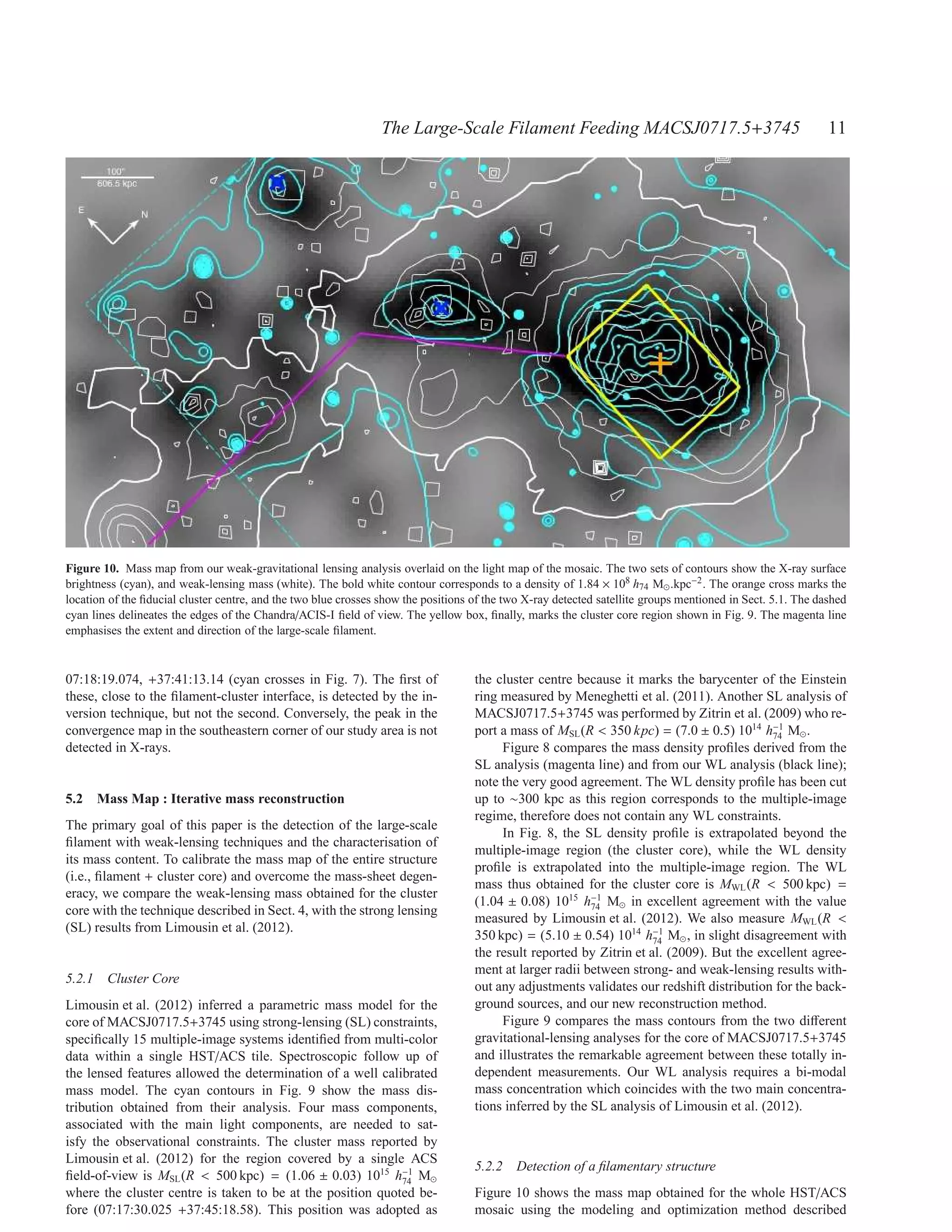
face mass density shown in Fig. 10. Its validity is confirmed by the We thank Douglas Clowe for accepting to review this paper and for
excellent agreement between the mass of the cluster core measured his useful comments. MJ would like to thank Graham P. Smith,
by us, MWL (R < 500 kpc) = (1.04 ± 0.08) × 1015 h−1 M⊙ , and the
74
Kavilan Moodley, and, Pierre-Yves Chabaud for useful discus-
one obtained in a strong-lensing analysis by Limousin et al. (2012), sions. EJ acknowledges support from the Jet Propulsion Labora-
MSL (R < 500 kpc) = (1.06 ± 0.03) × 1015 h−1 M⊙ .
74
tory under contract with the California Institute of Technology, the
Based on our weak-lensing mass reconstruction, we report the NASA Postdoctoral Program, and, the Centre National d’Etudes
first unambiguous detection of a large-scale filament fueling the Spatiales. MJ and EJ are indebted to Jason Rhodes for discus-
growth of a massive galaxy cluster at a node of the Cosmic Web. sions and advice. HE gratefully acknowledges financial support
The projected length of the filament is approximately 4.5 h−1 Mpc,
74
from STScI grant GO-10420. We thank the UH Time Allocation
and its mean mass surface density (2.92 ± 0.66) × 108 h74 M⊙ kpc−2 . Committee for their support of the extensive groundbased follow-
We measure the width and mass surface density of the filament as up observations required for this study. ML acknowledges the Cen-
a function of distance from the cluster centre, and find both to de- tre National de la Recherche Scientifique (CNRS) for its support.
crease, albeit with local variations due to at least four embedded The Dark Cosmology Centre is funded by the Danish National Re-
mild mass concentrations. One of these, at a projected distance of search Foundation. This work was performed using facilities of-
1.85 h−1 Mpc from the cluster centre, coincides with an X-ray de-
74
fered by CeSAM (Centre de donn´ eS Astrophysique de Marseille-
e
tected galaxy group. The filament is found to narrow at a cluster- (http://lam.oamp.fr/cesam/). This work was supported by World
centric distance of approximately 3.6 h−1 Mpc as it curves south
74
Premier International Research Center Initiative (WPI Initiative),
and, most likely, also recedes from us. We find the cluster’s mass MEXT, Japan.
surface density to decrease as r−2 until the onset of the filament
flattens the profile dramatically.
Following the analysis by Ebeling et al. (2012, in preparation)
REFERENCES
we adopt an average inclination angle with respect to the plane of
the sky of 75◦ for the majority of the filament’s length. For this sce- Arag´ n-Calvo M. A., van de Weygaert R., Jones B. J. T., van der
o
nario and under the simplifying assumption of a cylindrical cross- Hulst J. M., 2007, ApJ, 655, L5
section we obtain estimates of the filament’s three-dimensional Arnouts S., Cristiani S., Moscardini L., Matarrese S., Lucchin F.,
length and average mass density in units of the Universe’s criti- Fontana A., Giallongo E., 1999, MNRAS, 310, 540
cal density of 18 h−1 Mpc and (206 ± 46) ρcrit , respectively. How-
74 Arnouts S., Walcher C. J., Le F` vre O., Zamorani G., Ilbert O., Le
e
ever, additional systematic uncertainties enter since either quantity Brun V., Pozzetti L., Bardelli S., Tresse L., Zucca E., Charlot S.,
is sensitive to the adopted inclination angle. These values lie at the [...] 2007, A&A, 476, 137
high end of the range predicted from numerical simulations (e.g., Bertin E., Arnouts S., 1996, A&A, 117, 393

16. 16 M. Jauzac, E. Jullo, J.-P. Kneib, H. Ebeling, A. Leauthaud, C. J. Ma, M. Limousin, R. Massey, J. Richard
Bond J. R., Kofman L., Pogosyan D., 1996, Nature , 380, 603 E., Mobasher B., [...] 2009, ApJ, 690, 1236
Bond N. A., Strauss M. A., Cen R., 2010, MNRAS, 409, 156 Jullo E., Kneib J., 2009, MNRAS, 395, 1319
Casertano S., de Mello D., Dickinson M., Ferguson H. C., ´
Jullo E., Kneib J.-P., Limousin M., El´asd´ ttir A., Marshall P. J.,
ı o
Fruchter A. S., Gonzalez-Lopezlira R. A., Heyer I., Hook R. N., Verdugo T., 2007, New Journal of Physics, 9, 447
Levay Z., Lucas R. A., Mack J., Makidon R. B., Mutchler M., Kaastra J. S., Werner N., Herder J. W. A. d., Paerels F. B. S., de
Smith T. E., Stiavelli M., Wiggs M. S., Williams R. E., 2000, AJ, Plaa J., Rasmussen A. P., de Vries C. P., 2006, ApJ, 652, 189
120, 2747 Kaiser N., Wilson G., Luppino G., Kofman L., Gioia I., Metzger
Ceccarelli L., Paz D. J., Padilla N., Lambas D. G., 2011, MNRAS, M., Dahle H., 1998, ArXiv Astrophysics e-prints
412, 1778 Kartaltepe J. S., Ebeling H., Ma C. J., Donovan D., 2008, MNRAS,
Cen R., Ostriker J. P., 1999, ApJ, 519, L109 389, 1240
Clowe D., Luppino G. A., Kaiser N., Henry J. P., Gioia I. M., Kassiola A., Kovner I., 1993, ApJ, 417, 450
1998, ApJ, 497, L61+ Kneib J.-P., Ellis R. S., Smail I., Couch W. J., Sharples R. M.,
Colberg J. M., Krughoff K. S., Connolly A. J., 2005, MNRAS, 359, 1996, ApJ, 471, 643
272 Koekemoer A. M., Fruchter A. S., Hook R. N., Hack W., 2002, in
Colberg J. M., White S. D. M., Jenkins A., Pearce F. R., 1999, S. Arribas, A. Koekemoer, & B. Whitmore ed., The 2002 HST
MNRAS, 308, 593 Calibration Workshop : Hubble after the Installation of the ACS
Colless M., Dalton G., Maddox S., Sutherland W., Norberg P., and the NICMOS Cooling System MultiDrizzle: An Integrated
Cole S., Bland-Hawthorn J., Bridges T., Cannon R., Collins C., Pyraf Script for Registering, Cleaning and Combining Images.
Couch W., Cross N., [...] 2001, MNRAS, 328, 1039 pp 337–+
Cuesta A. J., Prada F., Klypin A., Moles M., 2008, MNRAS, 389, Le F` vre O., Vettolani G., Garilli B., Tresse L., Bottini D., Le
e
385 Brun V., Maccagni D., Picat J. P., Scaramella R., Scodeggio M.,
Diego J. M., Tegmark M., Protopapas P., Sandvik H. B., 2007, [] 2005, A&A, 439, 845
MNRAS, 375, 958 Leauthaud A., Finoguenov A., Kneib J., Taylor J. E., Massey R.,
Dietrich J. P., Schneider P., Clowe D., Romano-D´az E., Kerp J.,
ı Rhodes J., Ilbert O., Bundy K., Tinker J., George M. R., Capak
2005, A&A, 440, 453 P., [...] 2010, ApJ, 709, 97
Donovan D. A. K., 2007, PhD thesis, University of Hawai’i at Leauthaud A., Massey R., Kneib J., Rhodes J., Johnston D. E.,
Manoa Capak P., Heymans C., Ellis R. S., Koekemoer A. M., Le F` vre e
Ebeling H., Barrett E., Donovan D., 2004, ApJ, 609, L49 O., Mellier Y., [...] 2007, ApJS, 172, 219
Ebeling H., Barrett E., Donovan D., Ma C.-J., Edge A. C., van Leauthaud A., Tinker J., Bundy K., Behroozi P. S., Massey R.,
Speybroeck L., 2007, ApJ, 661, L33 Rhodes J., George M. R., Kneib J.-P., Benson A., Wechsler R. H.,
Ebeling H., Edge A. C., Henry J. P., 2001, ApJ, 553, 668 Busha M. T., Capak P., [] 2012, ApJ, 744, 159
Edge A. C., Ebeling H., Bremer M., R¨ ttgering H., van Haarlem
o Limousin M., Ebeling H., Richard J., Swinbank A. M., Smith
M. P., Rengelink R., Courtney N. J. D., 2003, MNRAS, 339, 913 G. P., Rodionov S., Ma C. ., Smail I., Edge A. C., Jauzac M.,
ı o ´
El´asd´ ttir A., Limousin M., Richard J., Hjorth J., Kneib J.-P., Jullo E., Kneib J. P., 2012, ArXiv e-prints
Natarajan P., Pedersen K., Jullo E., Paraficz D., 2007, ArXiv e- Limousin M., Kneib J.-P., Natarajan P., 2005, MNRAS, 356, 309
prints, 710 Limousin M., Richard J., Jullo E., Kneib J. P., Fort B., Soucail
Faber S. M., Jackson R. E., 1976, ApJ, 204, 668 G., El´asd´ ttir A., Natarajan P., Ellis R. S., Smail I., Czoske O.,
ı o
Fang T., Canizares C. R., Yao Y., 2007, ApJ, 670, 992 Smith G. P., Hudelot P., Bardeau S., Ebeling H., Egami E., Knud-
Fang T., Marshall H. L., Lee J. C., Davis D. S., Canizares C. R., sen K. K., 2007, ApJ, 668, 643
2002, ApJ, 572, L127 Lupton R., Gunn J. E., Ivezi´ Z., Knapp G. R., Kent S., 2001, in
c
Fritz A., Ziegler B. L., Bower R. G., Smail I., Davies R. L., 2005, F. R. Harnden Jr., F. A. Primini, & H. E. Payne ed., Astronomical
MNRAS, 358, 233 Data Analysis Software and Systems X Vol. 238 of Astronomi-
Galeazzi M., Gupta A., Ursino E., 2009, ApJ, 695, 1127 cal Society of the Pacific Conference Series, The SDSS Imaging
Gavazzi R., Mellier Y., Fort B., Cuillandre J.-C., Dantel-Fort M., Pipelines. pp 269–+
2004, A&A, 422, 407 Ma C., Ebeling H., 2010, MNRAS, pp 1646–+
Geller M. J., Huchra J. P., 1989, Science, 246, 897 Ma C.-J., Ebeling H., Barrett E., 2009, ApJ, 693, L56
Gray M. E., Taylor A. N., Meisenheimer K., Dye S., Wolf C., Ma C.-J., Ebeling H., Donovan D., Barrett E., 2008, ApJ, 684, 160
Thommes E., 2002, ApJ, 568, 141 Massey R., Bacon D., Refregier A., Ellis R., 2002, in N. Metcalfe
Hahn O., Carollo C. M., Porciani C., Dekel A., 2007, MNRAS, & T. Shanks ed., A New Era in Cosmology Vol. 283 of Astro-
381, 41 nomical Society of the Pacific Conference Series, Cosmic Shear
Heymans C., Gray M. E., Peng C. Y., van Waerbeke L., Bell E. F., with Keck: Systematic Effects. p. 193
Wolf C., Bacon D., Balogh M., Barazza F. D., Barden M., B¨ hm o Massey R., Heymans C., Berg´ J., Bernstein G., Bridle S., Clowe
e
A., Caldwell [] 2008, MNRAS, 385, 1431 D., Dahle H., Ellis R., Erben T., Hetterscheidt M., High F. W.,
Heymans C., Van Waerbeke L., Bacon D., Berge J., Bernstein G., Hirata C., [...] 2007, MNRAS, 376, 13
Bertin E., Bridle S., Brown M. L., Clowe D., Dahle H., Erben T., Massey R., Rhodes J., Leauthaud A., Ellis R., Scoville N.,
Gray M., [...] 2006, MNRAS, 368, 1323 Finoguenov A., 2006, in American Astronomical Society Meet-
Huchra J. P., Geller M. J., 1982, ApJ, 257, 423 ing Abstracts Vol. 38 of Bulletin of the American Astronomical
Ilbert O., Arnouts S., McCracken H. J., Bolzonella M., Bertin E., Society, A Direct View of the Large-Scale Distribution of Mass,
Le F` vre O., Mellier Y., Zamorani G., Pell` R., Iovino A., Tresse
e o from Weak Gravitational Lensing in the HST COSMOS Survey.
L., Le Brun V., [...] 2006, A&A, 457, 841 pp 966–+
Ilbert O., Capak P., Salvato M., Aussel H., McCracken H. J., Massey R., Stoughton C., Leauthaud A., Rhodes J., Koekemoer
Sanders D. B., Scoville N., Kartaltepe J., Arnouts S., Le Floc’h A., Ellis R., Shaghoulian E., 2010, MNRAS, 401, 371

17. The Large-Scale Filament Feeding MACSJ0717.5+3745 17
Mead J. M. G., King L. J., McCarthy I. G., 2010, MNRAS, 401,
2257
Meneghetti M., Fedeli C., Zitrin A., Bartelmann M., Broadhurst
T., Gottl¨ ber S., Moscardini L., Yepes G., 2011, A&A, 530,
o
A17+
Miyazaki S., Komiyama Y., Sekiguchi M., Okamura S., Doi M.,
Furusawa H., Hamabe M., Imi K., Kimura M., Nakata F., Okada
N., Ouchi M., Shimasaku K., Yagi M., Yasuda N., 2002, PASJ,
54, 833
Moody J. E., Turner E. L., Gott III J. R., 1983, ApJ, 273, 16
Novikov D., Colombi S., Dor´ O., 2006, MNRAS, 366, 1201
e
Oguri M., Hamana T., 2011, MNRAS, 414, 1851
Pimbblet K. A., Drinkwater M. J., 2004, MNRAS, 347, 137
Rasmussen J., 2007, ArXiv e-prints
Rhodes J., Refregier A., Groth E. J., 2000, ApJ, 536, 79
Rhodes J. D., Massey R. J., Albert J., Collins N., Ellis R. S., Hey-
mans C., Gardner J. P., Kneib J.-P., Koekemoer A., Leauthaud
A., Mellier Y., Refregier A., Taylor J. E., Van Waerbeke L., 2007,
ApJS, 172, 203
Rix H.-W., Barden M., Beckwith S. V. W., Bell E. F., Borch A.,
Caldwell J. A. R., H¨ ussler B., Jahnke K., Jogee S., McIntosh
a
D. H., Meisenheimer K., Peng C. Y., Sanchez S. F., Somerville
R. S., Wisotzki L., Wolf C., 2004, ApJS, 152, 163
Schneider P., King L., Erben T., 2000, A&A, 353, 41
Seitz C., Schneider P., 1995, A&A, 297, 287
Sheth R. K., Jain B., 2003, MNRAS, 345, 529
Skilling J., 1998, in G. J. Erickson, J. T. Rychert, & C. R. Smith
ed., Maximum Entropy and Bayesian Methods Massive Infer-
ence and Maximum Entropy. pp 1–+
Sousbie T., Pichon C., Courtois H., Colombi S., Novikov D.,
2006, ArXiv Astrophysics e-prints
Williams R. J., Mathur S., Nicastro F., Elvis M., 2007, ApJ, 665,
247
Williams R. J., Mulchaey J. S., Kollmeier J. A., Cox T. J., 2010,
ApJ, 724, L25
Wuyts S., van Dokkum P. G., Kelson D. D., Franx M., Illingworth
G. D., 2004, ApJ, 605, 677
Yess C., Shandarin S. F., 1996, ApJ, 465, 2
York D. G., Adelman J., Anderson Jr. J. E., Anderson S. F., An-
nis J., Bahcall N. A., Bakken J. A., Barkhouser R., Bastian S.,
Berman E., Boroski W. N., [...] 2000, AJ, 120, 1579
Zitrin A., Broadhurst T., Rephaeli Y., Sadeh S., 2009, ApJ, 707,
L102