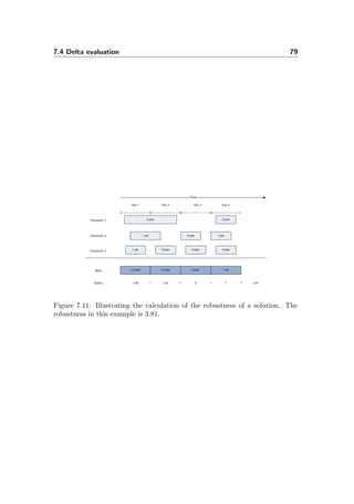
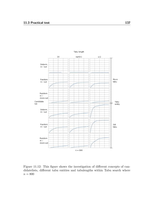
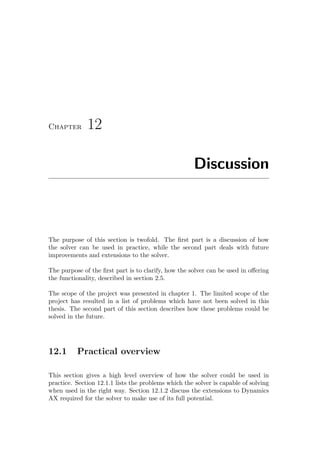
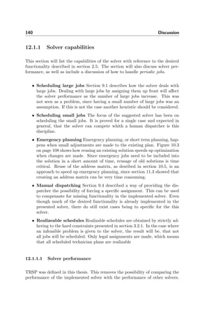
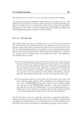
This thesis examines the Technician Routing and Scheduling Problem (TRSP) which involves scheduling service technicians. The thesis was conducted in collaboration with Microsoft, who was interested in developing software to automate technician scheduling. Through case studies of companies, a model of TRSP was developed based on operations research theory. A metaheuristic solver was implemented based on concepts like Tabu search and genetic algorithms. The solver was integrated with Microsoft Dynamics AX. Testing on real-world and random data showed the solver could create better schedules than human dispatchers according to key performance indicators. The solver improved all tested indicators.


![32 Complexity analysis of TRSP
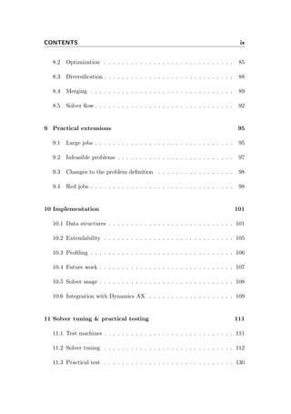
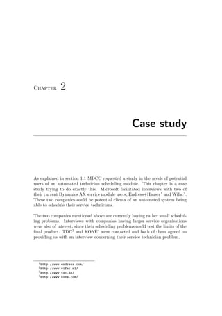
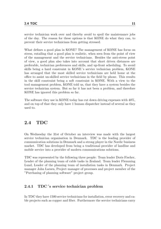
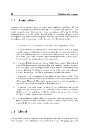
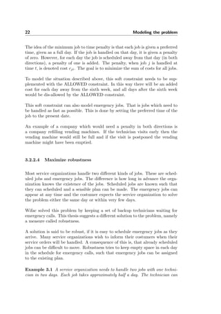
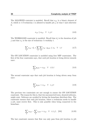
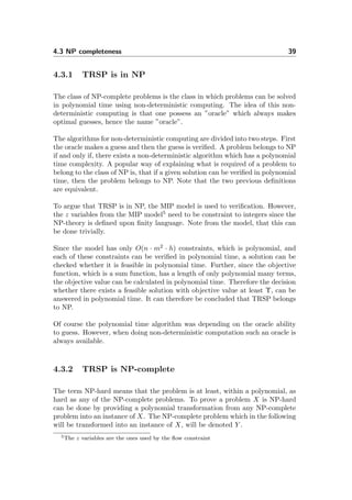
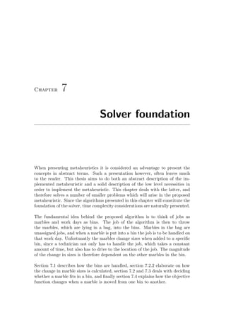
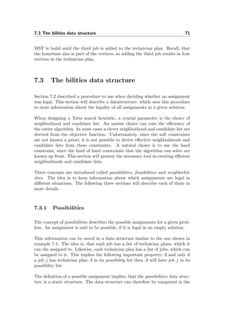
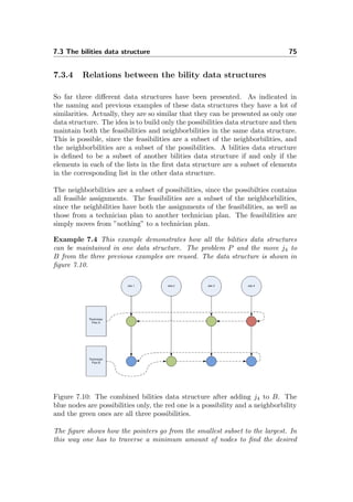
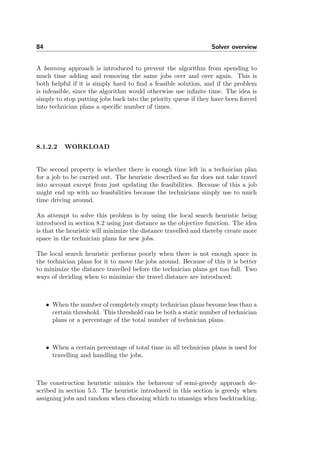
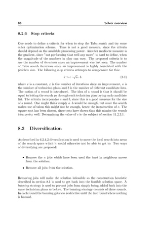
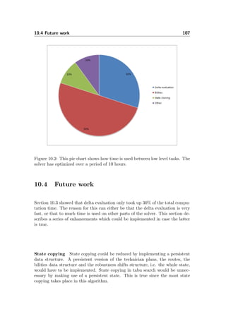
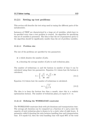
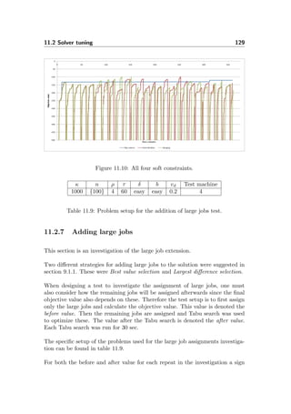
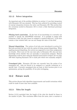
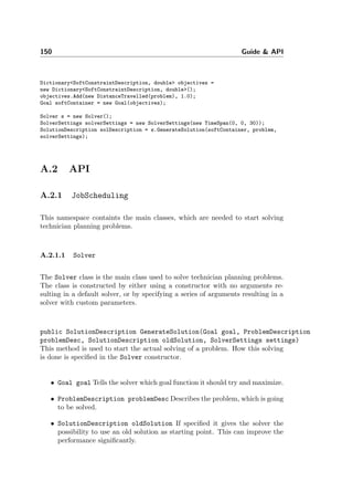
Figure 4.1: The computational effort used by the ILOG CPLEX solver as a
function of the problem size.
The size of problems solvable by using the MIP model is compared to the size
of real life problems. This is done to conclude that the MIP model does not
have any practical application for instances of TRSP. The case study can be
used when doing this. The interviewed company with the smallest problem is
Endress + Hauser. They have three technicians, they plan for a horizon of 20
days and within this period they handle 90 jobs.
Applying these data to the MIP model gives approximately 5 · 105
binary vari-
ables, which is 1000 times more binary variables than what the CPLEX solver
can handle. Therefore it can be concluded, that using a MIP model is not a
feasible approach in practice.
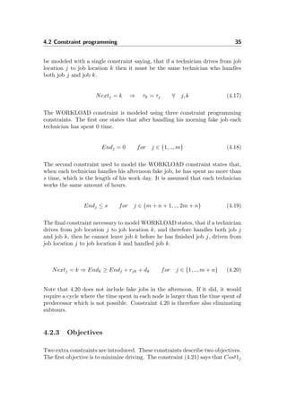
4.2 Constraint programming
This section models the problem as a Constraint programming (CP) model
and analyzes the efficiency of the Microsoft Optima CP solver. Constraint
Programming is an optimization framework. CP has the advantage over MIP
that logical operators such as implication can be used. Further, CP has a number
of special constraints such as alldifferent, which can be used to require a number
of variables to be different. The presented CP model is strongly inspired by the
model in [3]. In this section it is assumed that the horizon of the optimization
problem is only one day.](https://image.slidesharecdn.com/503dded7-6a67-40e0-a1a6-1f1df852e418-160708125022/85/ep08_11-44-320.jpg)
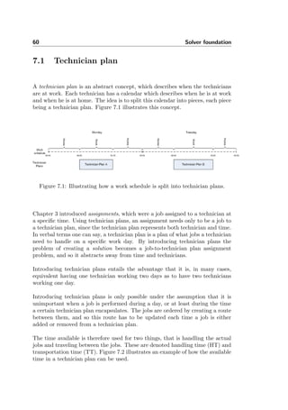
![40 Complexity analysis of TRSP
If Y can be transformed into X by a polynomial transformation, then solving X
only requires a polynomial larger effort than solving Y . Recall that a polynomial
transformation specifies two requirements. First, the time complexity of the
transformation must be bounded by a polynomial. Second, the size of the
output problem must only be a polynomial times larger than the input problem.
Since the transformation from Y to X is polynomial, Y can be solved by first
transforming it to an instance of X, and then solving X. To prove that X is
NP-hard, it is therefore sufficient to provide a polynomial transformation from
a known NP-complete problem Y into an instance of X.
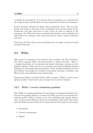
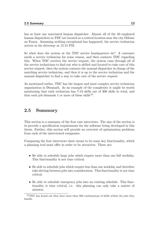
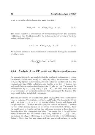
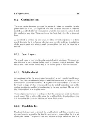
4.3.2.1 A polynomial transformation from TSP to TRSP
The transformation is made by exploiting that the Travelling Salesman Problem
is an instance of TRSP. TSP is NP-complete6
.
• Only one technician.
• The technician can handle all jobs.
• Only one day.
• The length of the day is set to infinity.
• αROB = αT T C = αJT T = 0, i.e. only driving is optimized.
The special instance of the TRSP model is stated using the notation from the
MIP-model. Note that the indices i and t are omitted since the problem only
contains one technician working one day. Further, the x variables are omitted
since obviously the only technician handles all jobs.
Min
j k
rjk · yjk
Such that:
j
yjk = 1 ∀ k
k
yjk = 1 ∀ j
k
zkj −
k
zjk = 1 ∀ j {homebase}
6See [6] pp. 453.](https://image.slidesharecdn.com/503dded7-6a67-40e0-a1a6-1f1df852e418-160708125022/85/ep08_11-52-320.jpg)
![42 Complexity analysis of TRSP
Such that:
i
xij = 1 ∀ j
j
xij · dj ≤ 1 ∀ i
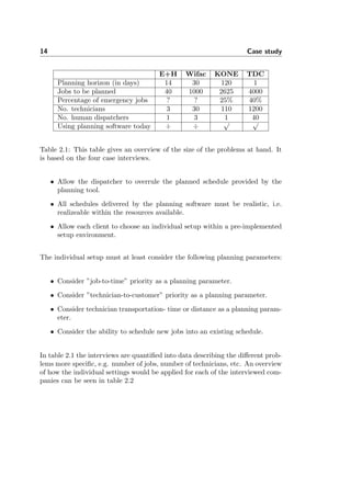
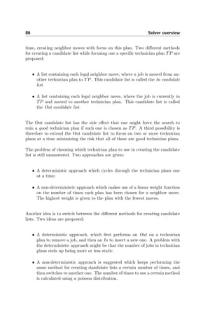
The above model is recognized as the BP since it is equivalent to maximize the
technicians not doing anything and minimizing the ones that are.
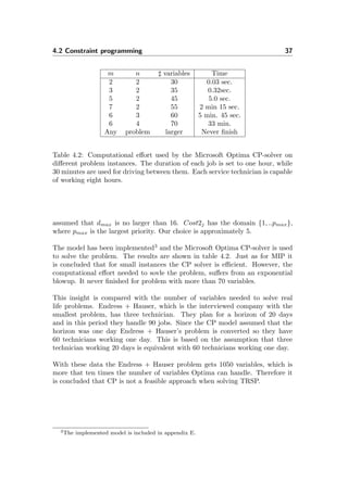
4.3.3 Real life instances of TRSP
It seems pretty obvious that even though both TSP and BP are components of
TRSP, neither of them are the instances real life planning problems will give rise
to. This section aims to analyze real life instances of TRSP and thereby extend
the understanding of TRSP, since the understanding is crucial when designing
algorithms.
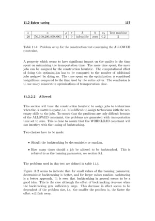
A constraint which was not used in neither TSP nor BP was the ALLOWED
constraint. The ALLOWED constraint can disallow a technician to handle a
job. If the A matrix is sparse, each job can only be handled by few technicians
on certain days. Therefore the ALLOWED constraint can significant reduce the
number of feasible solutions in the TRSP.
From the case interviews it seemed fair to assume, that no technician can handle
more than a few jobs on a single day due to the WORKLOAD constraint, i.e
the number of jobs handled by one technician on one day will not scale with the
problem size. Recall that the TSP was the instance of TRSP where one techni-
cian handled all jobs. Clearly each technician has to drive a Hamiltonian cycle
each day, i.e solve a TSP. However, these tours might be quite small. Designing
a very good heuristic for a general TSP might not be necessary. Instead one
should focus on developing fast algorithms for small instances of TSP. Further,
the WORKLOAD constraint could, like the ALLOWED constraint, reduce the
number of feasible solutions significant. This should be exploited in a good
TRSP algorithm.
BP seemed to have some relation with TRSP. There exists a quite good approx-
imation algorithm for BP namely the First Fit Decreasing algorithm7
denoted
FFD. The algorithm sorts the elements/jobs by size in increasing order and
then it assigns the jobs to the first bin where these fit. This algorithm has
a runtime of O(n · lg(n)) and a proven bound of 11/9·OPT + 6/9·bin, where
7[1] pp. 1-11](https://image.slidesharecdn.com/503dded7-6a67-40e0-a1a6-1f1df852e418-160708125022/85/ep08_11-54-320.jpg)

![Chapter 5
Metaheuristic concepts
Metaheuristics are optimization methods for solving computationally hard prob-
lems. Metaheuristics are used when wellknown standard solvers like the ILOG
CPlex solver cannot solve the problem at hand. This can happen if the in-
stance of the problem is either very large and or very complex. In [11] pp. 17 a
metaheuristic is defined as follows:
A meta-heuristic refers to a master strategy that guides and modifies
other heuristics to produce solutions beyond those that are normally
generated in a quest for local optimality. The heuristics guided by
such a meta-strategy may be high level procedures or may embody
nothing more than a description of available moves for transforming
one solution into another, together with an associated evaluation
rule.
If a meta-heuristic according to the definition is ”... a master strategy that guides
and modifies other heuristics...”, then one needs to know what a heuristic is.
According to [16] pp. 6, a heuristic is defined in the following way:
A heuristic is a technique which seeks good (i.e. near-optimal) solu-
tions at a reasonable computation cost without being able to guar-](https://image.slidesharecdn.com/503dded7-6a67-40e0-a1a6-1f1df852e418-160708125022/85/ep08_11-57-320.jpg)
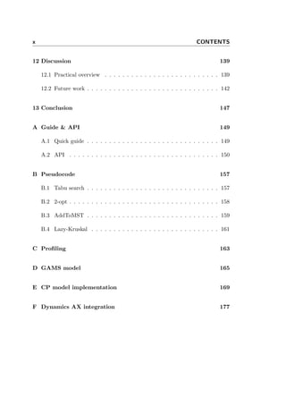
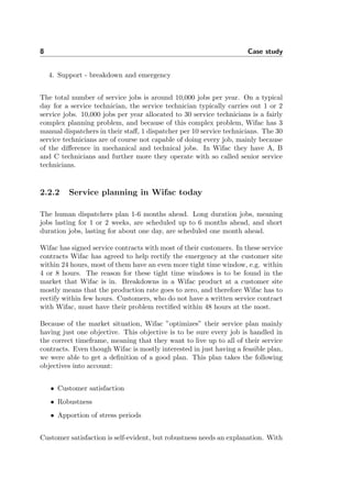
![5.2 Simulated annealing 47
to the solution that are larger than just the adjustment of a single decision
variable.
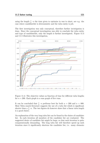
Most widely the value on the x-axis is interpreted as the value of a decision value.
A better interpretation of the x-axis in figure 5.1, when doing local search, is to
let the value of the axis be different neighbor solutions.
It is possible to extend the neighborhood, i.e. the set of neighbor solutions, so
one can guarantee that the Hill climber will find global optimum. Unfortunately,
the neighborhood needs to be extended so it´s exponential big and therefore it
ruins the idea of getting fast solutions.
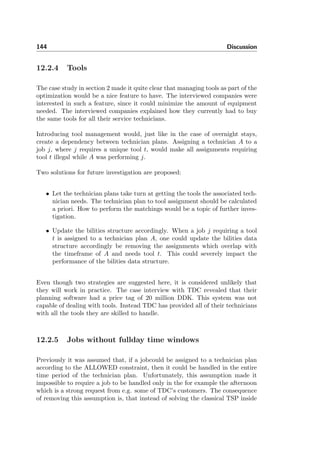
Figure 5.1: This figure is illustrating the concept of having more than one local
optimum. The green stars are illustrating where Hill climbing would get stuck
when maximizing the objective function, and the red stars are illustrating where
Hill climbing would get stuck when minimizing the objective function.
Since the problem with Hill climbing is that it often gets stuck in a local opti-
mum, the focus will be on search algorithms being able to avoid local optima.
5.2 Simulated annealing
The name and inspiration behind simulated annealing originate from metallurgy,
a technique involving heating and controlled cooling of a material to increase
size of its crystals and reduce their defects. First, heat causes atoms to become
unstuck from their initial positions (a local minimum of the internal energy)
and wander randomly through states of higher energy; then second, carefully
decreasing gives the atoms more chances of finding configurations with lower
internal energy than the initial one. [10] pp. 187. Simulated annealing is capable](https://image.slidesharecdn.com/503dded7-6a67-40e0-a1a6-1f1df852e418-160708125022/85/ep08_11-59-320.jpg)
![48 Metaheuristic concepts
of avoiding local optima by implementing the mentioned annealing process.
Simulated annealing is a neighbor search algorithm. In each iteration only one
neighbor solution is evaluated and then the move is either accepted or rejected.
If the move is an improving move it is always accepted, and if the move is non-
improving it is accepted with some probability. The probability with which non-
improving moves are accepted is calculated from a decreasing cooling function.
Therefore in the first iterations almost all moves are accepted and later on
almost all non-improving moves are rejected. Further, many implementations
also consider the magnitude of the change in the objective value when deciding
whether a non-improving move is accepted or not.
5.2.1 Pros & Cons
Advantages when using Simulated annealing are its simplicity and its ability
in preventing local optima. Simulated annealing can often provide high-quality
solutions, where no tailored algorithms are available [10] pp. 204. Further, it
is proven that Simulated anneling converges towards the optimal solution as
time goes to infinity [22]. Unfortunatly, no practical problem allows the use of
infinity time, so this property is only of theoretical interest.
The main disadvantage when using Simulated annealing is first and foremost
the computation time needed to obtain high-quality solutions. This is a con-
sequence of the lack of prioritization of neighbor solutions, since only one is
evaluated. Furthermore, it is often difficult to guess a good cooling scheme. If
the temperature is too high; Simulated annealing behaves as Random search,
and if the tempature is to low, Simulated annealing will behave as Hill climb-
ing. In most cases the cooling function needs to fit the specific problem and
especially the objective function.
5.3 Genetic algorithms
Genetic algorithms is the best known type of evolutionary algorithms. An evo-
lutionary algorithm is a generic population-based metaheuristic optimization
algorithm. These algorithms are inspired by biological evolution: reproduction,
mutation, recombination and selection. The typical structure, described in [10]
pp. 98, of how to implement a Genetic algorithm is:
1. Generate initial population.](https://image.slidesharecdn.com/503dded7-6a67-40e0-a1a6-1f1df852e418-160708125022/85/ep08_11-60-320.jpg)
![5.6 Choosing a metaheuristic for TRSP 51
5.6 Choosing a metaheuristic for TRSP
This thesis aims at developing a metaheuristic. A metaheuristic is the product
of a series heuristics as explained in the first paragraph. This section is a
discussion of concepts which are going to be included in the heuristic proposed
in this thesis.
Section 1.1 described Microsofts interest in being able to provide their clients
with emergency handling of new arriving jobs. The running time of the meta-
heuristic to be chosen is therefore a very important factor when choosing among
the introduced heuristic concepts. Further, one cannot be certain which soft
constraints the clients will find useful and so very little information about the
objective function is available. Both of these arguments are strong disadvantages
when using Simulated annealing, and therefore this heuristic is discarded.
TRSP have many similarities wiht VRP as stated in section 4.3.3. Tabu search
has a history of provided state of the art solutions to VRP, and so it seems quite
intuitive to investigate Tabu search further. Tabu seach is the best metaheuristic
at finding good solutions fast since it is initially quite simular to hill climbing.
This is important since emergency planning was one of the requirements stated
in the case study.
A main difference between TRSP and VRP are the ease at which feasible solu-
tion are obtained. VRP can obtain a feasible solution by simple sending each
costumer a separate vehicle. This is not the case for TRSP since one does
not necessarily posses enough service technicians to do this. A construction
algorithm is therefore needed.
T-Cluster and T-Sweep are examples of construction heuristics for VRP. As
explained in [18] pp. 897 both of these algorithms are greedy algorithm which
assigns costumers to vehicles after their geographical position. The ALLOWED
constraint can, if the A matrix is sparse, make both of these construction algo-
rithm diffucult to use. If the A matrix is sparse it is more important to find a
service technicain who can handle critical jobs than obtain a plan where jobs
are assigned by their geographical position.
A greedy construction approach is chosen, since it seems that there is no tailored
algorithm for obtaining feasible solutions to TRSP. The semi-greedy construc-
tion concept is used as the basis of this algorithm. The proposed construction
algorithm will not make use of iterative constructions. The algorithm is how-
ever still going to use non-determinism. This is the case since, if a deterministic
construction fail to find a feasible solution, then randomness can be used as a
way of searching for less greedy solutions.](https://image.slidesharecdn.com/503dded7-6a67-40e0-a1a6-1f1df852e418-160708125022/85/ep08_11-63-320.jpg)
![54 Introduction to Tabu search
6.2 Concepts
6.2.1 Search space
The search space is the set of all possible solutions the local search can visit.
The name ”search space” arises from the following metaphor; if you consider
the variation of a cost function to be a landscape of potential solutions to a
problem where the height of each feature represents its cost.
In general the search space will have at least the size of the feasible space since
it would be unwise to eliminate possible good (or optimal) solutions from the
search. The reason for applying a metaheuristic is when a problem is computa-
tionally hard, i.e. the feasible space is enormous.
Defining the search space can for some problems seem very obvious, but that is
not always so. Sometimes it is not a good idea to restrict the search space to
feasible solutions, several cases have shown that a move to an infeasible solution
can be a very good idea. Today several methods of allowing infeasible solutions
in the search space exist, i.e. ”Constraint Relaxation” or ”Strategic Oscillation”.
[10] pp. 169.
6.2.2 Neighborhood
Assume an element in the search space x, i.e. a solution. Then all the possible
transformations of x leading to another solution in the search space, are defined
as neighbors of x. All the possible single transformations of x together define the
entire neighborhood of x. This leads to the conclusion that the neighborhood
is a subset of the search space.
The Operation research literature states over and over, that choosing a search
space and a neighborhood structure is by far the most critical step in the design
phase of the Tabu search algorithm.
6.2.3 Short term memory
In this section focus will be on short term memory. Candidate list strategies and
the tabu list are examples of short term memory. The name short term memory
is derived from the usage of candidate lists and the tabu list, since both of them](https://image.slidesharecdn.com/503dded7-6a67-40e0-a1a6-1f1df852e418-160708125022/85/ep08_11-66-320.jpg)
![6.2 Concepts 55
only consider the recently achieved knowledge.
6.2.3.1 Candidate list
When determining which neighbor to move along to from an existing solution,
the candidate list holds the neighbors that are to be investigated, meaning that
the candidates of x is a subset of the neighbors of x. Three good motivators for
making use of candidate list:
• The first motivation for building candidate lists is the observation that
both the efficiency and efficacy of a search can be greatly influenced by
isolating good candidate moves.
• The second motivation comes from the need to reduce the computing time
needed for evaluation, i.e. when objective value is expensive to calculate.
• The third motivation comes from the possibility of exploiting the problem
structure, meaning that particular problems lead to special constructions
of intelligent candidate lists1
.
6.2.3.2 Tabu list
The tabu list is a list containing entities from the latest chosen neighbors. There-
fore when considering future moves, the reverse move of the performed one is
deemed tabu.
Tabu tenure is the way of keeping track of the status of move attributes that
compose tabu restrictions and more important, when these restrictions are ap-
plicable. Through history several ways of doing this have been proposed. This
section will explain the most commonly used tabu tenures according to the lit-
erature. The rules of tabu tenures can be divided into two classifications, the
static and the dynamic tenures.
The static rules are defined as ones where the tabu list length remains fixed
throughout the entire search. For example a constant length of between 7 and
20, or a degressive growing function in the number of decision variables like
example
√
n where n is a measure of the problem size. [16, p. 94].
1Context related rules.](https://image.slidesharecdn.com/503dded7-6a67-40e0-a1a6-1f1df852e418-160708125022/85/ep08_11-67-320.jpg)
![56 Introduction to Tabu search
The dynamic rules are defined as the ones where the tabu list length vary
throughout the search. For instance a length that randomly or systematically
varies between some static lower and upper bound. More intelligent dynamic
tabu lists can be used to create a more advanced variation, such as long tabu lists
when few improvements can be found. A problem with the dynamic approaches
is that they are very problem dependant.
One way to make the tabu lists more effective is to make use of the a so-called
aspiration criteria.
6.2.3.3 Aspiration criteria
When a move is performed and an intity therefore is declaired tabu, this will
result in more than one solution being tabu. Some of these solutions being
tabu could be of excellent quality, and this is where this aspiration criteria has
its strength. The aspiration criteria is introduced to remove moves from the
tabu list. The most commonly used aspiration criteria, [16] pp. 98, is called
”Aspiration by Objective”. The idea is to remove solutions which have a better
objective value than the currently best known from the tabu list.
Further reading regarding aspiration criteria can be found on pp. 100 in [16]
and on pp. 50 in [11].
6.2.4 Longer Term Memory
Small term memory can be considered as temporary knowledge. Longer term
memory differs from this by encapsulating information from the entire search.
In some Tabu search implementations, the short term memory components are
sufficient to produce high quality solutions. The use of longer term memory does
usually not require very much runtime before the improvements starts becoming
visible. The reason for this success in long term strategies is to be found in the
modified neighborhoods produced by Tabu search; these may contain solutions
not in the original one or combinations of elite solutions leading to even better
solutions. According to [11] pp. 93, the fastest method for some types of routing
and scheduling problems, are based on longer term memory.](https://image.slidesharecdn.com/503dded7-6a67-40e0-a1a6-1f1df852e418-160708125022/85/ep08_11-68-320.jpg)
![6.2 Concepts 57
6.2.4.1 Intensification
Intensification is a strategy to modify or change the solution in a way that
seems to be historically good. The idea in intensification resembles the strategy
a human being would make use of. When a part a of solution reappears over
and over again, it might be worth keeping this part of the solution and then
focus on the remaining part of the solution.
Another classical intensification method is the intensification-by-restart method,
which takes the best solution so far, and restarts from there, meaning that the
tabu list is cleared. [11] pp. 96.
6.2.4.2 Diversification
As mentioned earlier in this thesis, one of the main problems with the Tabu
search algorithm is the tendency of being to local. To avoid the algorithm
being to local, diversification is imposed. The observation is that Tabu search
tends to spend most, if not all, of its time in a restricted part of the search
space when making use of only short term memory. The consequence with the
algorithm being to local is that even though it returns good solutions, it might
fail to explore the most interesting parts of the search space. As opposed to
other metaheuristics as for example Genetic algorithms where randomization in
combining population elements provides diversification to the algorithm, Tabu
search has no natural way of diversifying except from the special case where the
tabu list is very long.
Diversification is created to drive the search into new regions of the search space.
One very common diversification strategy is to bring infrequently seen entities
into the solution. This approach forces the algorithm into hopefully new region
of the search space and thereby improve the solution. [11] pp. 98.](https://image.slidesharecdn.com/503dded7-6a67-40e0-a1a6-1f1df852e418-160708125022/85/ep08_11-69-320.jpg)


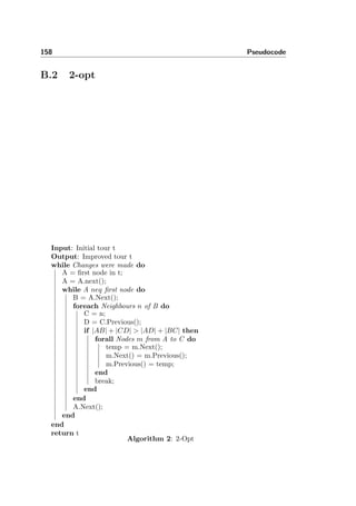
![7.2 Checking legality 67
the number of near nodes can be bounded by a constant, the algorithm has a
time complexity of O(k). The pseudocode of the implemented algorithm can
be seen in appendix B and rigorous proofs for both correctness and the time
complexcity can be found in [20].
The problem concerning removing a job location from a MST is more compli-
cated than the adding problem. However, like the adding problem there exists
a linear algorithm. Unfortunately, this algorithm requires to keep a geometric
structure such as Delaunay triangulation [20]. Further, the time complexity
contains some large constants. Therefore it was in a TRSP context considered
to be faster to build a new MST each time a job was being removed from a
technician plan.
To build MST, Kruskal’s algorithm1
is used. Kruskal’s algorithm first sorts
the edges by cost. Then the edges are added to the MST one at a time in
increasing order. Each edge is only added, if it does not result in a cycle. When
implementing Kruskal, two tricks can be used. The first trick is to use Quick-
Sort2
to sort the edges. Then a lazy approach where only the edges smaller than
the pivot element are sorted recursively, the recursive calls sorting the elements
larger than the pivot element are stored in a stack until needed. This is possible
since Kruskal in each iteration, only needs the edge with the lowest cost. The
second trick is, that the check for cycles is moved into the sorting algorithm so
that edges which will result in a cycle are not sorted but simply discarded. This
could increase the speed, since not all the sorting is done before starting adding
edges to the MST.
The runtime of the Lazy-Kruskal’s algorithm is O(k2
· lg(k)), where k is the
number of vertices, like the standard algorithm since it is not believed that any
of the introduced tricks gives an asymptotic improvement.
The pseudocode of the implemented algorithm can be seen in appendix B.
The proof of correctness for the Lazy-Kruskal algorithm is similar to the proof
of the traditional Kruskal algorithm. I.e after the p’th iteration the p cheapest
edges that do not result in a cycle are chosen. Therefore after the k−1 iteration,
a complete MST is build. It is certain that for each iteration, no cycle is created
since only edges are added to the MST if the two vertices associated with the
edge are not members of the same disjoint set.
1[21] page 569
2[21] page 146](https://image.slidesharecdn.com/503dded7-6a67-40e0-a1a6-1f1df852e418-160708125022/85/ep08_11-79-320.jpg)
![68 Solver foundation
7.2.2 TSP Heuristics
If the transportation time bounds does not provide sufficient information to
answer the question: Whether it is legal to assign job j to technician plan A?
One could determine a good or optimal solution to the TSP and then declare the
assignment legal if the tour is sufficient cheap. Note that if the optimal TSP-
tour is calculated, the question can be answered with certainty, else a heuristic
answer is given.
The largest difference between optimal and near-optimal algorithms to TSP,
is that optimal has an exponential time complexity and guarantee optimality
whereas near-optimal algorithms often have polynomial time complexities, and
if a guarantee is given, this is mostly to weak to be used practical. Ergo, a time
versus quality trade off has to be made.
When TRSP was analyzed in chapter 4, it was concluded that the number
of jobs in each technician plan was small which could argue for an optimal
algorithm. However, this thesis is developing a system which should be as
general as possible, meaning many different clients should be able to use it.
Even though the interviewed clients only have a small number of jobs in each
technician plan, this does not mean that potential future clients does. Note
that the consequence of choosing an optimal algorithm will be an exponential
blow up in computational effort within the engine. Therefore, the choice in
this thesis will be to use a heuristic where the time complexity can be bounded
polynomial. However, the consequense of choosing a heuristic is that the answer
to the question concerning time within the technician plan might end up with
a false negative. This consequence is accepted.
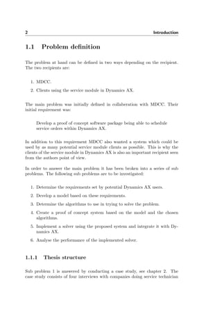
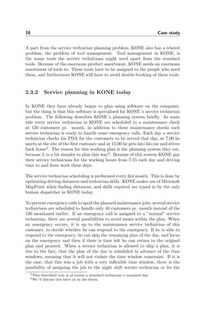
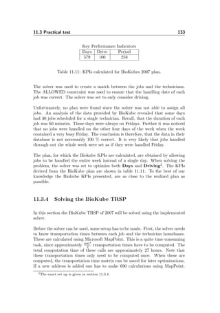
As stated in [15] and [12], the state of the art TSP heuristics are Lin-Kernighan
and a number of other metaheuristics. However, a much simpler heuristic, 2-
opt, is considered a faster alternative, this can be concluded by the results
presented in table 7.1 which is part of the results presented in the downloadable
preliminary version of the chapter in [12], pp. 215-310. The quality of the
heuristics presented in the table, is based on the Held Karp lower bounds.
Since it could be the case that a TSP needs to be solved each time it is checked
whether it is legal to assign a job to a technician plan, computational runtimes
are weighted higher than quality. Therefore 2-opt, based on the results presented
in table 7.1, will be the chosen heuristic to solve instances of TSP in TRSP when
bounds does not provide sufficient information.](https://image.slidesharecdn.com/503dded7-6a67-40e0-a1a6-1f1df852e418-160708125022/85/ep08_11-80-320.jpg)
![7.2 Checking legality 69
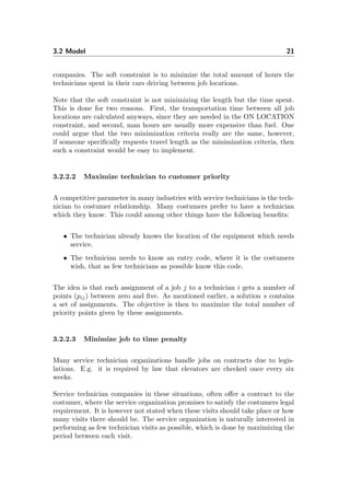
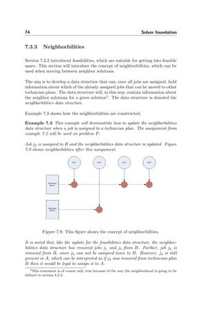
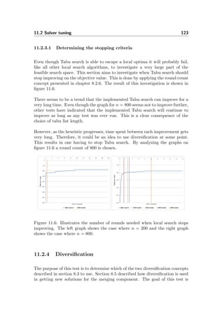
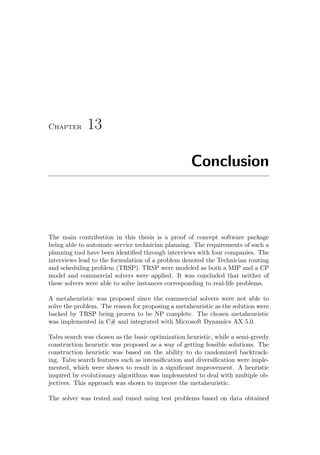
Algo.N 102
102.5
103
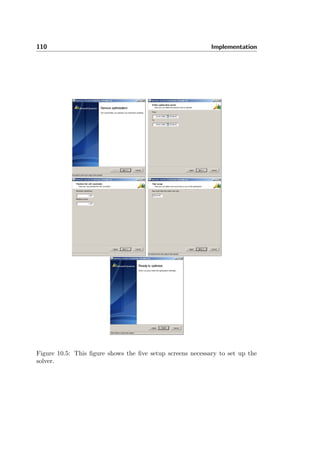
2-Opt 4.5% 0.03 s. 4.8% 0.09 s. 4.9% 0.34 s.
3-Opt 2.5% 0.04 s. 2.5% 0.11 s. 3.1% 0.41 s.
LK 1.5% 0.06 s. 1.7% 0.20 s. 2.0% 0.77 s.
Table 7.1: This table provides results on several heuristics for solving TSP, the
percent excess the percentive value over the Held-Karp lower bound and the
other is the computational time used to find the result.
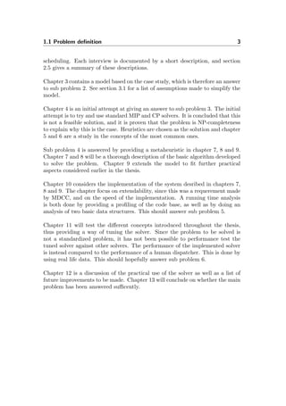
2-Opt
The 2-Opt algorithm was first proposed by Croes in 1958, although the basics
of the algorithm had already been suggested by Flood in 1956 [12]. The 2-opt
algorithm is a tour improvement algorithm. I.e the input is a Hamiltonian tour
and the output is, if the algorithm can find one, a shorter Hamiltonian tour.
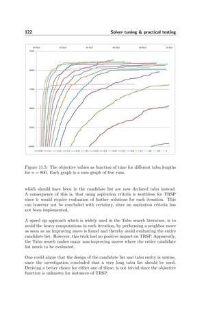
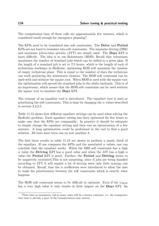
The idea Floods came up with, was to break the tour into two paths, and then
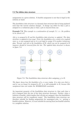
reconnect those paths into the other possible way, see figure 7.6.
Figure 7.6: This figure shows the principle of 2-Opt.
As seen on figure 7.6, the idea is to take two pairs of consecutive nodes from
a tour, here the pairs A & B and C & D. Check and see if the distances
|AB| + |CD| is larger than the distances |AC| + |DB|. If |AB| + |CD| distance
is the largest, then swap A and C which will result in a reversed tour between
those two nodes.
The 2-opt algorithm tries all possible swaps. If an improvement is found, the
swap is made and the algorithm is restarted. The time complexity of 2-Opt
is equal to the number of improvements times the computational effort of one
improvement. One improvement can in worst case require O(k2
), where k is
the number of jobs in the technician plan, if no improvement is found and all
combinations of swaps are tried. The number of improvements is trickier. It
has been proven in [13] that there exist instances and starting tours such that](https://image.slidesharecdn.com/503dded7-6a67-40e0-a1a6-1f1df852e418-160708125022/85/ep08_11-81-320.jpg)


![10.1 Data structures 103
root is the head of the set. This implementation does not provide efficient worst
case bounds on all operations since the Find-Set operation can require linear
work. However, in amortized sense the Find-Set operation is fast since it does
some repair work which is prepaid by the Union operation. Two tricks which
speed up the operations are used. The first trick is union by rank. The idea
is that the smaller tree should be attached to the larger tree when performing
Union. This is done to make the traversal from the leaf to the root in the Find-
Set operation as short as possible. The rank of each node in the tree cannot be
updated in constant time. However, the rank can be bound upwards, and this
upper bound provides sufficient information to allow the amortized analysis to
work. The second trick is path compression. Since the Find-Set operation has
to visit each node on the path from from a start node to the root, then one
could simply maintain the root pointers when visiting the nodes on the way to
the root.
The amortized analysis use a potential function which stores potential in the
data structure according to the sum of rank for the whole forest. This means that
potential is stored in the data structure when performing the Union operation,
which can later be used to run from a node to the root and do path compression.
The pseudocode and a rigorous proof for the time complexity can be found in
[21] page 508. The analysis concludes that n disjoint set operations on a data
structure containing m elements require amortized work equal to O(n · α(m)),
where α(m) is the inverse Ackermann function. This function is constant for all
practical purposes.
10.1.3 Priority Queue
A priority queue is used in the construction algorithm to keep track of the
unassigned jobs. The jobs in the priority queue are prioritized after a ”critical
to assign” measure which describes how many technician plans a specific job
can be assigned to. An important insight from the construction algorithm is,
that each time a job is assigned to a technician plan all jobs in the feasibility
list of that technician plan have to be updated since their critical value may
have changed. This results in a lot of Update Key operations each time a single
Extract Min operation is performed. The priority queue has been implemented
by using a Splay tree since this data structure provides amortized O(lg(n))
running time for these two operations.
A Splay tree is a binary search tree. Whereas most binary search trees, such
as Red-Black trees and AVL trees, guarantee their performance by maintaining
(almost) perfect balance, Splay trees guarantee their performance using amor-](https://image.slidesharecdn.com/503dded7-6a67-40e0-a1a6-1f1df852e418-160708125022/85/ep08_11-115-320.jpg)
![104 Implementation
tization. The idea is that operations are allowed to require much work only if
they are balancing the search tree at the same time, and in this way making
future operations faster.
The balancing in splay trees are done by an operation called Splaying. A Splay
operation consists of a sequence of double rotations. A double rotation involves
three nodes and are performed to do a local balancing between these three nodes.
This balancing results in the total height of the search tree being decreased by
one in enough of these rotations for the amortized analysis to work. A sequence
of rotations where one node is rotated all the way to the root is denoted a Splay.
The potential function used in the amortized analysis is a function that sum
up the size of each possible sub tree. Therefore a balanced tree will have less
potential than an unbalanced one, and since splaying balances the tree a long
search in the splay tree will be paid by the succeeding splay.
A rigorous analysis of the time complexity and pseudocode for all the operations
can be found in [19]. The analysis concludes that all operations on a Splay tree
with n nodes require O(lg(n)) amortized work.
A very nice property of the splay tree node is that recently touched nodes will be
located near the root and will therefore be cached. This is a consequence of the
Splay operation. Recall that the most time consuming part of the construction
algorithm was the backtracking where nodes with low critical value were pushed
back into the priority queue. It can be expected that the Splay tree will provide
high efficiency in the construction algorithm since the Extract-Min operation
will be fast when the element with low critical value is located near the top.
Note that since each operation on a Splay tree with n elements has a time
complexity of O(lg(n)), sorting m elements can by done by first adding each
element and then extracting min m times. This will take O(m · lg(m)) time
which is proven to be optimal for any comparison sorting algorithm1
. The splay
tree is used for sorting in certain cases throughout the implementation.
The Insert operation can be improved by using a lazy strategy. This improve-
ment results in the operation only requiring constant amortized work. This
improvement will however not improve the construction algorithm since a series
of Update Key operations, which contains one Remove and one Insert, is always
followed by a Extract Min which will make the lazyness indifferent.
Another benefit of the Splay tree is that it is quite easy to implement.
1See [21] page 167.](https://image.slidesharecdn.com/503dded7-6a67-40e0-a1a6-1f1df852e418-160708125022/85/ep08_11-116-320.jpg)
![10.6 Integration with Dynamics AX 109
10.6 Integration with Dynamics AX
The solver has been integrated in Dynamics AX through the use of a dynamic
linked libary2
. This is possible since Dynamics AX has CLR interoperability
meaning that .NET objects can by instantiated inside Dynamics AX using the
X++ language3
. The X++ code integrating the solver dll with the Dynamics
AX application can be found in appendix F.
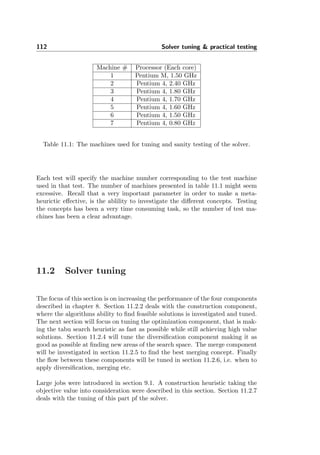
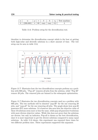
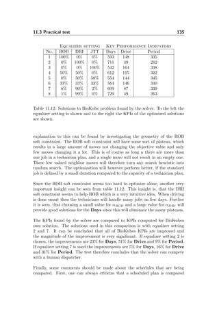
The user starts the solver by going through a small wizard. Figure 10.5 shows
the steps necessary to set up the solver. Figure 10.4 shows how a dispatch board
is used to visually show the assignment of service jobs in Dynamics AX. The
dispatch board can therefore be used to show the result of a solver optimization.
Figure 10.4: This dispatch board shows a schedule with three jobs.
2I.e. a .NET managed code .dll file.
3See [5] for more on the workings of Dynamics AX and the X++ language.](https://image.slidesharecdn.com/503dded7-6a67-40e0-a1a6-1f1df852e418-160708125022/85/ep08_11-121-320.jpg)


![Appendix A
Guide & API
A.1 Quick guide
This section contains a small guide in using the solver.
The first example shows how to construct and solve a small problem with 1
technician and 1 job.
Schedule schedule = new Schedule();
schedule.AddPeriod(new TimeFrame(60 * 9, 60 * 15));
Technician tech = new Technician("Peter", schedule, new Address("Jagtvej 69",
"København N", "2200", "Denmark"));
Technician[] techs = new Technician[] { tech };
JobDescription job = new JobDescription("Fix elevator", 60 * 2, new TimeFrame(0,
60 * 24), new Address("Strandboulevarden 100", "København Ø", "2100", "Denmark"));
JobDescription[] jobs = new JobDescription[] { job };
TechnicianSkills skills = new TechnicianSkills();
skills.addSkill(tech, job);
HardConstraint[] constraints = new HardConstraint[] { skills };
ProblemDescription problem = new ProblemDescription(techs, jobs, new Assignment[0],
new TimeFrame(0, 60 * 24), constraints);](https://image.slidesharecdn.com/503dded7-6a67-40e0-a1a6-1f1df852e418-160708125022/85/ep08_11-161-320.jpg)
![152 Guide & API
• Address Where the job is going to be performed.
• Timeframe The period of time in which the job is allowed to be performed.
A.2.2.4 ProblemDescription
This class describes a problem. A ProblemDescription is constructed from the
following arguments:
• Technician[] techs An array of the technicians in the problem.
• JobDescription[] greenJobs An array of the jobs, which are going to
be performed by the technicians.
• Assignment[] redJobs An array of jobs which are forced to be performed
by a specific technician at a specific time.
• HardConstraint[] hardConstraints The constraints which can’t be vi-
olated. This could be technician skill levels.1
• Dictionary<Address, Dictionary<Address, int>> distanceMatrix A
matrix with the distance in minutes between each address in the problem
to each of the other addresses. If this argument isn’t specified then the
class calls MapPoint and gets it to calculate the matrix. If there are a
large number of jobs in the problem, then MapPoint might take a while to
calculate this matrix, so it might be a good idea to calculate the matrix
offline.
A.2.2.5 Schedule
A Schedule describes a technicians timeschedule. The schedule is by default
totally empty. The class contains two methods:
public void AddPeriod(TimeFrame period) Adds the timeperiod period
to the schedule.
1See TechnicianSkills section A.2.4.2.](https://image.slidesharecdn.com/503dded7-6a67-40e0-a1a6-1f1df852e418-160708125022/85/ep08_11-164-320.jpg)


![B.4 Lazy-Kruskal 161
B.4 Lazy-Kruskal
Input: Graph G - G is an array containing the edges in a graph
Output: MST T
T = ∅;
foreach vertex v in G do
Make-Set(v);
end
push Lazy-QuickSort(G,1, length(G)) into Call-Stack
while size(T) < (# of vertices in G -1 ) do
e = pop Call-Stack;
T = T e;
Union(head(e),tail(e));
end
return T
Algorithm 5: Lazy-Kruskal
Input: Array of edges G, position in G start, position in G end
Output: smallest edge between position start and end in G
while true do
if start < end then
smaller size, larger size = Partition(G,start,end);
Push Lazy-QuickSort(G, end - larger size, end) into Call-Stack;
Push Lazy-QuickSort(G, start, start + smaller size) into
Call-Stack;
end
else if Find-Set(head(start) = Find-Set(tail(start)) then
return G[start];
end
pop Call-Stack;
end
Algorithm 6: Lazy-QuickSort
Input: Array of edges G, position in G start , position in G end
Output: smaller size, larger size
pivot = G[random number between start and end] ;
smaller size =0 ;
larger size = 0 ;
foreach j in G from start to (end - larger size) do
if G[j] < pivot and Find-Set(head(j) = Find-Set(tail(j)) then
swap in G(j, start + smaller size);
smaller size = smaller size + 1;
end
else if G[j] ≥ pivot and Find-Set(head(j) = Find-Set(tail(j)) then
swap in G(j, end - larger size);
larger size = larger size + 1;
j = j-1 ;
end
end
return larger size, smaller size](https://image.slidesharecdn.com/503dded7-6a67-40e0-a1a6-1f1df852e418-160708125022/85/ep08_11-173-320.jpg)


![Appendix E
CP model implementation
Listing E.1: CP model implementation using Optima
1 using System;
2 using System.Collections.Generic;
3 using System.Text;
4 using Microsoft.Planning.Solvers;
5 using System.IO;
6
7 namespace CPSolver
8 {
9 class Program
10 {
11 static void Main(string [] args)
12 {
13 SolveOurProblem ();
14 }
15
16 public static void SolveOurProblem ()
17 {
18 FileInfo mainFile = new FileInfo(" CPSolverTest .txt");
19 using ( StreamWriter sw = new StreamWriter (mainFile.OpenWrite ()))
20 {
21 Random r = new Random (2132);
22
23 int [] nArray = new int[] { 1, 2, 3, 4, 5, 6, 7 };
24 int [] mArray = new int[] { 2, 3, 4, 5 };
25
26 for (int a = 0; a < mArray.Length; a++)
27 {
28 for (int b = 0; b < nArray.Length; b++)
29 {
30 for (int c = 0; c < 5; c++) // Repeats
31 {](https://image.slidesharecdn.com/503dded7-6a67-40e0-a1a6-1f1df852e418-160708125022/85/ep08_11-181-320.jpg)
![170 CP model implementation
32 DateTime startTime = DateTime.Now;
33
34 int n = nArray[b]; // Number of jobs
35 int m = mArray[a]; // Number of TP ’s
36
37 int tp_size = 6*m + (int)((3 * n) / (double)m);
// 200
38
39 int x_max = 4;
40 int y_max = 4;
41
42 double skills = 1;
43 int p_max = 4; // Max prioritet værdi
44 int t_max = 4; // Max skrue
45
46 int d_max = (int)Math.Sqrt(Math.Pow(x_max , 2) +
Math.Pow(y_max , 2)); ;
47
48 int [][] jobPoint = new int[2 * m + n][];
49 int [] homePoint = new int [2] { r.Next(x_max), r.
Next(y_max) };
50
51 {
52 for (int i = 0; i < jobPoint.Length; i++)
53 {
54 jobPoint[i] = new int [2];
55
56 if (i < m || i >= m + n)
57 {
58 jobPoint[i][0] = homePoint [0];
59 jobPoint[i][1] = homePoint [1];
60 }
61 else
62 {
63 jobPoint[i][0] = r.Next(x_max);
64 jobPoint[i][1] = r.Next(y_max);
65 }
66 }
67 }
68
69 int [][] v_ij = new int[m][];
70 {
71 for (int y = 0; y < v_ij.Length; y++)
72 {
73 v_ij[y] = new int[2 * m + n];
74 }
75
76 for (int y = 0; y < v_ij.Length; y++)
77 {
78 for (int t = 0; t < v_ij[y]. Length; t++)
79 {
80 if (t < m || t >= m + n)
81 {
82 v_ij[y][t] = 1;
83 }
84 else
85 {
86 if (skills >= r.NextDouble ())
87 {
88 v_ij[y][t] = 1;
89 }
90 else
91 {
92 v_ij[y][t] = 0;
93 }](https://image.slidesharecdn.com/503dded7-6a67-40e0-a1a6-1f1df852e418-160708125022/85/ep08_11-182-320.jpg)
![171
94 }
95 }
96 }
97 }
98
99 int [][] d_jk = new int[2 * m + n][];
100 {
101 for (int i = 0; i < d_jk.Length; i++)
102 {
103 d_jk[i] = new int[2 * m + n];
104 }
105
106 for (int i = 0; i < d_jk.Length; i++)
107 {
108 for (int j = i; j < d_jk[i]. Length; j++)
109 {
110 int dist = (int)Math.Sqrt(Math.Pow(
jobPoint[i][0] - jobPoint[j][0] ,
2) + Math.Pow(jobPoint[i][1] -
jobPoint[j][1] , 2));
111 d_jk[i][j] = dist;
112 d_jk[j][i] = dist;
113 }
114 }
115 }
116
117
118 int [][] p_ji = new int[m][];
119
120 for (int t = 0; t < p_ji.Length; t++)
121 {
122 p_ji[t] = new int[2 * m + n];
123
124 for (int y = 0; y < p_ji[t]. Length; y++)
125 {
126 if (m <= y && y < m + n)
127 {
128 p_ji[t][y] = 1 + r.Next(p_max); // 1
or 2
129 }
130 }
131 }
132
133 int [] t_j = new int[2 * m + n];
134
135 for (int t = 0; t < t_j.Length; t++)
136 {
137 if (m <= t && t < m + n)
138 {
139 t_j[t] = 1 + r.Next(t_max); // 0 or 1
140 }
141 }
142
143 FiniteSolver S = new IntegerSolver (null , null);
144
145 using (S) // This disposes S after use
146 {
147 ValueSet small_j = S. CreateInterval (1, m);
148 ValueSet large_j = S. CreateInterval (m + n +
1, 2 * m + n);
149 ValueSet middlelarge_j = S. CreateInterval (m +
1, 2 * m + n);
150
151 ValueSet i = S. CreateInterval (1, m);](https://image.slidesharecdn.com/503dded7-6a67-40e0-a1a6-1f1df852e418-160708125022/85/ep08_11-183-320.jpg)
![172 CP model implementation
152 ValueSet j = S. CreateInterval (1, 2 * m + n);
// j is the jobs plus start and end for
each tp
153 ValueSet time = S. CreateInterval (0, tp_size);
// The time to use.
154
155 // Creating the 3 variables
156 Term [] R = S. CreateVariableVector (j, "R_", 2
* m + n);
157 Term [] Q = S. CreateVariableVector (time , "Q_",
2 * m + n);
158 Term [] Tau = S. CreateVariableVector (i, "Tau_"
, 2 * m + n);
159
160 // Creating the 2 objective variables
161 Term [] goal1 = S. CreateVariableVector (S.
CreateInterval (-d_max , 0), "goal1_", 2 *
m + n);
162 Term [] goal2 = S. CreateVariableVector (S.
CreateInterval (0, p_max), "goal2_", 2 *
m + n);
163
164
165 // Creating the constraints
166 // 1
167 S. AddConstraints (S.Unequal(R));
168
169
170 // 2
171 foreach (int t in small_j.Forward ())
172 {
173 S. AddConstraints (S.Equal (0, Q[t - 1]));
174 }
175
176 // 3
177 foreach (int t in large_j.Forward ())
178 {
179 S. AddConstraints (S.Equal(tp_size , Q[t -
1]));
180 }
181
182 // 4
183 foreach (int t in j.Forward ())
184 {
185 foreach (int k in middlelarge_j .Forward ()
)
186 {
187 S. AddConstraints (S.Implies(S.Equal(k,
R[t - 1]), S. GreaterEqual (Q[k -
1], Q[t - 1] + d_jk[t - 1][k -
1] + t_j[k - 1])));
188 }
189 }
190
191 // 5
192 foreach (int t in j.Forward ())
193 {
194 foreach (int y in i.Forward ())
195 {
196 if (v_ij[y - 1][t - 1] == 0)
197 {
198 S. AddConstraints (S.Unequal(y, Tau
[t - 1]));
199 }
200 }](https://image.slidesharecdn.com/503dded7-6a67-40e0-a1a6-1f1df852e418-160708125022/85/ep08_11-184-320.jpg)
![173
201 }
202
203 // 6
204 foreach (int t in small_j.Forward ())
205 {
206 S. AddConstraints (S.Equal(t, Tau[t - 1]));
207 }
208
209 // 7
210 foreach (int t in large_j.Forward ())
211 {
212 S. AddConstraints (S.Equal(t - (m + n), Tau
[t - 1]));
213 }
214
215 // 8
216 foreach (int t in large_j.Forward ())
217 {
218 S. AddConstraints (S.Equal(t - (m + n), R[t
- 1]));
219 }
220
221 // 9
222 foreach (int t in j.Forward ())
223 {
224 foreach (int k in j.Forward ())
225 {
226 S. AddConstraints (S.Implies(S.Equal(k,
R[t - 1]), S.Equal(Tau[k - 1],
Tau[t - 1])));
227 }
228 }
229
230 // The two objective constraints
231
232
233 foreach (int t in j.Forward ())
234 {
235 foreach (int k in j.Forward ())
236 {
237 S. AddConstraints (S.Implies(S.Equal(k,
R[t - 1]), S.Equal(-d_jk[t -
1][k - 1], goal1[t - 1]))); //
the objective is drive away from
238 }
239 }
240
241 foreach (int t in j.Forward ())
242 {
243 foreach (int y in i.Forward ())
244 {
245
246 S. AddConstraints (S.Implies(S.Equal(y,
Tau[t - 1]), S.Equal(p_ji[y -
1][t - 1], goal2[t - 1])));
247 }
248 }
249
250
251 Term [] goals = new Term[goal1.Length + goal2.
Length ];
252 goal1.CopyTo(goals , 0);
253 goal2.CopyTo(goals , goal1.Length);
254
255 // Creating the objective](https://image.slidesharecdn.com/503dded7-6a67-40e0-a1a6-1f1df852e418-160708125022/85/ep08_11-185-320.jpg)
![174 CP model implementation
256 S. TryAddMinimizationGoals (S.Neg(S.Sum(goals))
);
257
258 Dictionary <Term , int > bestSoln = null;
259 foreach (Dictionary <Term , int > soln in S.
EnumerateSolutions ())
260 {
261 bestSoln = soln;
262 }
263
264 if (bestSoln == null)
265 {
266 Console.WriteLine("No solution found");
267 }
268 /* else
269 {
270 PrintSol (R, Q, Tau , goal1 , goal2 ,
bestSoln );
271 }*/
272
273 // calculate obj value
274 int obj = 0;
275 int obj1 = 0;
276 int obj2 = 0;
277
278
279 for (int t = 0; t < 2 * m + n; t++)
280 {
281 obj1 += bestSoln[goal1[t]];
282 obj2 += bestSoln[goal2[t]];
283 }
284 obj = obj1 + obj2;
285
286
287 /* Console . WriteLine (" Obj1 :" + obj1);
288 Console . WriteLine (" Obj2 :" + obj2);
289 Console . WriteLine (" Obj :" + obj);
290
291 Console . WriteLine (" Done ");*/
292 }
293
294 TimeSpan timeUsed = DateTime.Now - startTime;
295
296 Console.WriteLine("n: " + n + " m: " + m + " time
: " + timeUsed. TotalSeconds );
297
298 sw.WriteLine(n + ";" + m + ";" + timeUsed.
TotalMilliseconds );
299 sw.Flush ();
300 }
301 }
302 }
303 }
304 }
305
306 private static void PrintSol(Term [] R, Term [] Q, Term [] Tau , Term []
goal1 , Term [] goal2 , Dictionary <Term , int > soln)
307 {
308 Console.WriteLine("TAU:");
309 for (int tau = 0; tau < Tau.Length; tau ++)
310 {
311 Console.WriteLine(tau +1 + ": " + soln[Tau[tau ]]);
312 }
313
314 Console.WriteLine("R:");](https://image.slidesharecdn.com/503dded7-6a67-40e0-a1a6-1f1df852e418-160708125022/85/ep08_11-186-320.jpg)
![175
315 for (int h = 0; h < R.Length; h++)
316 {
317 Console.WriteLine(h+1 + ": " + soln[R[h]]);
318 }
319
320 Console.WriteLine("Q:");
321 for (int h = 0; h < Q.Length; h++)
322 {
323 Console.WriteLine(h + 1 + ": " + soln[Q[h]]);
324 }
325
326 Console.WriteLine("Cost1:");
327 for (int h = 0; h < goal1.Length; h++)
328 {
329 Console.WriteLine(h + 1 + ": " + soln[goal1[h]]);
330 }
331
332 Console.WriteLine("Cost2:");
333 for (int h = 0; h < goal2.Length; h++)
334 {
335 Console.WriteLine(h + 1 + ": " + soln[goal2[h]]);
336 }
337 }
338 }
339 }](https://image.slidesharecdn.com/503dded7-6a67-40e0-a1a6-1f1df852e418-160708125022/85/ep08_11-187-320.jpg)

![Appendix F
Dynamics AX integration
Listing F.1: X++ class ServiceOptimize
1 public class ServiceOptimize
2 {
3 JobScheduling .Struct.TimeFrame wholeperiod;
4 utcdatetime starttime;
5
6 public void new( utcdatetime _starttime , utcdatetime _endtime )
7 {
8 starttime = _starttime;
9 wholeperiod = new JobScheduling .Struct.TimeFrame (0, this.
convertTime(_endtime));
10 }
11
12 JobScheduling .Struct. SolutionDescription optimize( JobScheduling .
SoftConstraints .Goal goal , JobScheduling .Struct.
ProblemDescription probDesc , int timeInSec)
13 {
14 JobScheduling .Struct. SolutionDescription solution;
15 JobScheduling .Solver solver = new JobScheduling .Solver ();
16 JobScheduling . SolverSettings settings = new JobScheduling .
SolverSettings (new System.TimeSpan (0, 0, timeInSec));
17
18 solution = solver. GenerateSolution (goal , probDesc , settings);
19 return solution;
20 }
21
22 void updateDatabase ( JobScheduling .Struct. SolutionDescription solDesc)
23 {
24 int length;
25 JobScheduling .Struct.Assignment [] assigns;
26 int i;
27 JobScheduling .Struct.Assignment assignment;](https://image.slidesharecdn.com/503dded7-6a67-40e0-a1a6-1f1df852e418-160708125022/85/ep08_11-189-320.jpg)
![178 Dynamics AX integration
28 JobScheduling .Struct. JobDescription job;
29 JobScheduling .Struct.Technician tech;
30 int time;
31 str jobDesc;
32 boolean b;
33 str techName;
34 utcdatetime timeFrom;
35 utcdatetime timeTo;
36 int duration;
37
38 smmActivities activities;
39 smmActivityParentLinkTable linkTable;
40
41 ttsbegin;
42 while select forupdate activities join linkTable
43 where activities. ActivityNumber == linkTable.
ActivityNumber &&
44 linkTable.RefTableId == tablenum( SMAServiceOrderLine )
45 {
46 assigns = solDesc. get_AssignmentArray ();
47 length = assigns.get_Length ();
48
49 b = false;
50 for (i = 0; i < length; i++)
51 {
52 assignment = assigns.GetValue(i);
53 job = assignment.get_Job ();
54 jobDesc = job. get_Description ();
55 if (jobDesc == activities. ActivityNumber )
56 {
57 tech = assignment. get_Technician ();
58 time = assignment.get_Time ();
59 techName = tech.get_Name ();
60 b = true;
61 break;
62 }
63 }
64
65 if (!b)
66 {
67 // Do nothing
68 }
69 else
70 {
71 duration = job. get_Duration ();
72 timeFrom = DateTimeUtil :: addMinutes(starttime
, time);
73 timeTo = DateTimeUtil :: addMinutes(starttime ,
duration + time);
74
75 activities. ResponsibleEmployee = techName;
76 activities. StartDateTime = timeFrom;
77 activities.EndDateTime = timeTo;
78 activities.update ();
79 }
80 }
81 ttscommit;
82 }
83
84 JobScheduling .Struct. ProblemDescription createProblemDescription ()
85 {
86 JobScheduling .Struct.Technician [] techs;
87 JobScheduling .Struct. JobDescription [] greenJobs;
88 JobScheduling .Struct.Assignment [] redJobs;](https://image.slidesharecdn.com/503dded7-6a67-40e0-a1a6-1f1df852e418-160708125022/85/ep08_11-190-320.jpg)
![179
89 JobScheduling . HardConstraints . HardConstraint []
hardConstraints ;
90 JobScheduling .Struct.TimeFrame period;
91 JobScheduling .Struct. ProblemDescription probDesc;
92 JobScheduling .Struct. AddressMatrix matrix;
93 System.IO.FileInfo addrFile;
94 int i;
95 int length;
96 str name;
97 JobScheduling .Struct. JobDescription jobDesc;
98 JobScheduling .Struct.Technician technician;
99 ;
100
101 addrFile = new System.IO.FileInfo("C: addrMatrix.txt");
102 /*
103 * Getting the data from the database .
104 */
105 techs = this. findTechnicians ();
106 this. findCalendars (techs);
107 greenJobs = this.findJobs ();
108 redJobs = new JobScheduling .Struct.Assignment [0](); // No red
jobs.
109 hardConstraints = new JobScheduling . HardConstraints .
HardConstraint [0](); // No extra hard constraints .
110
111 print "Loading the address matrix";
112 /*
113 * Creating the address matrix .
114 */
115 matrix = JobScheduling . AddressMatrixLoader :: Load(addrFile);
116 matrix = new JobScheduling .Struct. AddressMatrix (techs ,
greenJobs , redJobs , matrix);
117 JobScheduling . AddressMatrixLoader :: Save(addrFile , matrix);
118
119 print "Finished loading the address matrix";
120 /*
121 * Finally creating the problem description ...
122 */
123 probDesc = new JobScheduling .Struct. ProblemDescription (techs ,
greenJobs , redJobs , wholeperiod , hardConstraints ,
matrix);
124
125 return probDesc;
126 }
127
128 JobScheduling .Struct.Technician [] findTechnicians ()
129 {
130 Array techs = new Array(Types :: Class);
131 JobScheduling .Struct.Technician [] toBeReturned ;
132 JobScheduling .Struct.Technician tech;
133 JobScheduling .Struct.Address techAddress ;
134
135 int i = 1;
136 int returnLength ;
137
138 /*
139 * Tables
140 */
141 EmplTable emplTable;
142 DirPartyAddressRelationship
dirPartyAddressRelationship ;
143 DirPartyAddressRelationshipMapping
dirPartyAddressRelationshipMapping ;
144 Address address;
145 ;](https://image.slidesharecdn.com/503dded7-6a67-40e0-a1a6-1f1df852e418-160708125022/85/ep08_11-191-320.jpg)
![180 Dynamics AX integration
146
147 while select emplTable join DirPartyAddressRelationship join
DirPartyAddressRelationshipMapping join Address
148 where emplTable. DispatchTeamId != ’’ &&
149 DirPartyAddressRelationshipMapping .
RefCompanyId == Address.dataAreaId
&&
150 DirPartyAddressRelationshipMapping .
AddressRecId == Address.RecId &&
151 DirPartyAddressRelationshipMapping .
PartyAddressRelationshipRecId ==
DirPartyAddressRelationship .RecId &&
152 EmplTable.PartyId
==
DirPartyAddressRelationship .PartyId
153 {
154 // info( strfmt ("%1 , %2", emplTable .EmplId , Address .
Address ));
155
156 techAddress = new JobScheduling .Struct.Address(
Address.Street , Address.City , Address.ZipCode ,
Address. CountryRegionId );
157 tech = new JobScheduling .Struct.Technician(emplTable.
EmplId , new JobScheduling .Struct.Schedule (),
techAddress);
158
159 techs.value(i, tech);
160
161 i++;
162 }
163
164 print "#techs found:";
165 print i-1;
166
167 toBeReturned = new JobScheduling .Struct.Technician[i -1]();
168 returnLength = toBeReturned .get_Length ();
169
170 for (i = 0; i < returnLength ; i++)
171 {
172 toBeReturned .SetValue(techs.value(i+1), i);
173 }
174
175 return toBeReturned ;
176 }
177
178 JobScheduling .Struct. JobDescription [] findJobs ()
179 {
180 int duration;
181 JobScheduling .Struct.Address address;
182 JobScheduling .Struct. JobDescription job;
183
184 JobScheduling .Struct. JobDescription [] toBeReturned ;
185 Array jobs = new Array(Types :: Class);
186 int i = 1;
187 int returnLength ;
188
189 /*
190 * Tables
191 */
192 EmplTable emplTable;
193 smmActivities activities;
194 smmActivityParentLinkTable linkTable;
195 SMAServiceOrderLine serviceLine;
196 SMAServiceOrderTable serviceOrder ;
197 ;](https://image.slidesharecdn.com/503dded7-6a67-40e0-a1a6-1f1df852e418-160708125022/85/ep08_11-192-320.jpg)
![181
198
199 while select emplTable join activities join linkTable join
serviceLine join serviceOrder
200 where emplTable. DispatchTeamId != ’’ && empltable.
CalendarId != ’’ &&
201 activities. ResponsibleEmployee == emplTable
.EmplId &&
202 activities. ActivityNumber == linkTable.
ActivityNumber &&
203 linkTable.RefTableId == tablenum(
SMAServiceOrderLine ) &&
204 serviceLine.ActivityId == activities.
ActivityNumber &&
205 serviceLine. ServiceOrderId == serviceOrder .
ServiceOrderId
206
207 {
208 // info( strfmt ("%1 %2 %3 %4", activities .
ActivityNumber , activities . StartDateTime ,
activities . EndDateTime , serviceOrder .
ServiceAddress ));
209
210 duration = this.convertTime(activities.EndDateTime) -
this. convertTime (activities. StartDateTime );
211 address = new JobScheduling .Struct.Address(
serviceOrder .ServiceAddressStreet , serviceOrder .
ServiceAddressCity , serviceOrder .
ServiceAddressZipCode , serviceOrder .
ServiceAddressCountryRegion );
212 job = new JobScheduling .Struct. JobDescription (
activities.ActivityNumber , duration , wholeperiod
, address);
213
214 jobs.value(i, job);
215 i++;
216 }
217
218 print "#jobs found:";
219 print i-1;
220
221 toBeReturned = new JobScheduling .Struct. JobDescription [i -1]()
;
222 returnLength = toBeReturned .get_Length ();
223 for (i = 0; i < returnLength ; i++)
224 {
225 toBeReturned .SetValue(jobs.value(i+1) , i);
226 }
227
228 return toBeReturned ;
229 }
230
231 void findCalendars ( JobScheduling .Struct.Technician [] techs)
232 {
233 JobScheduling .Struct.Schedule s;
234 JobScheduling .Struct.Technician t;
235
236 utcdatetime timeFrom;
237 utcdatetime timeTo;
238 int fromInt;
239 int toInt;
240
241 int length;
242 int indx;
243 str techName;
244 JobScheduling .Struct.TimeFrame techFrame;](https://image.slidesharecdn.com/503dded7-6a67-40e0-a1a6-1f1df852e418-160708125022/85/ep08_11-193-320.jpg)
![183
296 s.AddPeriod(techFrame
);
297 break;
298 }
299 }
300 }
301 }
302 }
303 }
304
305 int convertTime( utcdatetime dtime)
306 {
307 int64 diff = DateTimeUtil :: getDifference (dtime , starttime);
308
309 int diffInMinutes = diff / 60;
310
311 return diffInMinutes ;
312 }
313 }
Listing F.2: Method called by the the wizard when pressing finish
1 public void closeOk ()
2 {
3 JobScheduling .Struct. SolutionDescription solDesc;
4 JobScheduling .Struct. ProblemDescription probDesc;
5 JobScheduling . SoftConstraints .Goal goal;
6 int i;
7 int length;
8 JobScheduling .Struct.Assignment [] assArray;
9 JobScheduling .Struct.Assignment assign;
10 JobScheduling .Struct. JobDescription jobDesc;
11 ServiceOptimize serviceOptimizer ;
12 utcdatetime fromTime;
13 utcdatetime toTime;
14 ;
15
16 super ();
17
18 // utcdatetime format : 2008 -01 -29 T13 :38:47
19 fromTime = fromDateTime . dateTimeValue ();
20 toTime = toDateTime. dateTimeValue ();
21
22 serviceOptimizer = new ServiceOptimize (fromTime , toTime);
23
24 print "Starting the creation of the problem description ";
25 probDesc = serviceOptimizer . createProblemDescription ();
26 print "The creation of the problem description ended";
27
28 goal = new JobScheduling . SoftConstraints .Goal ();
29 goal. AddConstraint (new JobScheduling . SoftConstraints . DistanceTravelled (
probDesc), travelField .realValue ());
30 goal. AddConstraint (new JobScheduling . SoftConstraints .Robustness(probDesc ,
120) , robustField.realValue ());
31 print "Starting the optimization ";
32 solDesc = serviceOptimizer .optimize(goal , probDesc , optiTime.value ());
33 print " Optimization ended";
34
35 info(solDesc. GetLongString ());
36
37 print "Updating the database";
38 serviceOptimizer . updateDatabase (solDesc);
39 }](https://image.slidesharecdn.com/503dded7-6a67-40e0-a1a6-1f1df852e418-160708125022/85/ep08_11-195-320.jpg)

![Bibliography
[1] Combinatorics, Algorithms, Probabilistic and Experimental Methodologies,
chapter The Tight Bound of First Fit Decreasing Bin-Packing Algorithm
Is FFD(I)≤11/9·OPT(I)+6/9. Springer Berlin / Heidelberg, 2007.
[2] Le Pape Claude Nuijten Wim Baptiste, Philippe. Constraint-Based
Scheduling Applying Constraint Programming to Scheduling Problems.
Kluwer Academic Publishers, London, 2001.
[3] Filippo Focacci, Andrea Lodi, and Michela Milano. A hybrid exact algo-
rithm for the tsptw. INFORMS J. on Computing, 14(4):403–417, 2002.
http://dx.doi.org/10.1287/ijoc.14.4.403.2827.
[4] Robert Ghanea-Hercock. Applied Evolutionary Algorithms in Java. Black-
well Scientific Publications, New York, New York, 2003.
[5] Olsen et al Greef, Pontoppidan. Inside Microsoft Dynamics AX 4.0. Mi-
crosoft Press, Redmond, Washington, 2006.
[6] John E. Hopcroft, Rajeev Motwani, Rotwani, and Jeffrey D. Ullman. In-
troduction to Automata Theory, Languages and Computability. Addison-
Wesley Longman Publishing Co., Inc., Boston, MA, USA, 2000.
[7] M. R. Garey & D. S. Johnson. COMPUTERS AND INTRACTABILITY
- A Guide to the Theory of NP-Completeness. Murray Hill, San Francisco,
California, 1979.
[8] R. A. Johnson. Miller & Freund´s Probability and Statistics for Engineers.
Prentice-Hall, London, 2000.](https://image.slidesharecdn.com/503dded7-6a67-40e0-a1a6-1f1df852e418-160708125022/85/ep08_11-197-320.jpg)
![186 BIBLIOGRAPHY
[9] P. J. Stuckey K. Marriott. Programming with Constraints - An Introduction.
The MIT Press, Cambridge, Massachusetts, 2001.
[10] E. K. Burke & G. Kendall. SEARCH METHODOLOGIES - Introductory
Tutorials in Optimization and Decision Support Techniques. Springer, New
York, New York, 2005.
[11] F. Glover & M. Laguna. TABU SEARCH. Kluwer Academic Publishers,
Norwell, Massachusetts, 1997.
[12] E. H. L. Aarts & J. K. Lenstra. Local Search in Combinatorial Optimization.
Princeton University Press, London, 1997.
[13] G. Lueker. manuscript. Princeton University, 1976.
[14] Irvin J. Lustig and Jean-Fran¸cois Puget. Program does not equal program:
Constraint programming and its relationship to mathematical program-
ming. Interfaces, 31(6):29–53, 2001. http://dx.doi.org/10.1287/inte.
31.7.29.9647.
[15] C. Nilsson. Heuristics for the traveling salesman problem. http://www.
ida.liu.se/~TDDB19/reports_2003/htsp.pdf.
[16] C. R. Reeves. Modern Heuristic Techniques for Combinatorial Problems.
Blackwell Scientific Publications, London, 1993.
[17] MAURICIO G.C. RESENDE. Greedy randomized adaptive search pro-
cedures (grasp). AT&T Labs Research Technical Report, 2001. http:
//www.research.att.com/~mgcr/doc/sgrasp.pdf.
[18] Stephan Scheuerer. A tabu search heuristic for the truck and trailer routing
problem. Comput. Oper. Res., 2006. http://dx.doi.org/10.1016/j.cor.
2004.08.002.
[19] Robert E. Sleator, Daniel D. & Tarjan. Self-adjusting binary search trees.
Journal of the Association for Computing Machinery, 1985. http://www.
cs.cmu.edu/~sleator/papers/self-adjusting.pdf.
[20] Mike Soss. Online construction of a minimal spanning tree (mst). http:
//cgm.cs.mcgill.ca/~soss/geometry/online_mst.html, 1997.
[21] R. L. Rivest & C. Stein T. H. Cormen, C. E. Leisersoon. Introduction to
Algorithms. The MIT Press, Cambridge, Massachusetts, 2001.
[22] J.P. Rasson V. Granville, K. Krivanek. Simulated annealing: A proff of
convergence. PATTERN ANALYSIS AND MACHINE INTELLIGENCE,
1994, (vol. 16, No. 6) pp. 652-656. http://doi.ieeecomputersociety.
org/10.1109/34.295910.](https://image.slidesharecdn.com/503dded7-6a67-40e0-a1a6-1f1df852e418-160708125022/85/ep08_11-198-320.jpg)
![BIBLIOGRAPHY 187
[23] David H. Wolpert and William G. Macready. No free lunch theorems
for search. Technical Report SFI-TR-95-02-010, Santa Fe, NM, 1995.
citeseer.ist.psu.edu/wolpert95no.html.](https://image.slidesharecdn.com/503dded7-6a67-40e0-a1a6-1f1df852e418-160708125022/85/ep08_11-199-320.jpg)

![BIBLIOGRAPHY 189
[11] [10] [5] [7] [21] [6] [12] [16] [4] [8] [2] [9] [19] [15] [17] [18] [22] [14] [13] [3]
[23] [1] [20]](https://image.slidesharecdn.com/503dded7-6a67-40e0-a1a6-1f1df852e418-160708125022/85/ep08_11-201-320.jpg)