The document is a technical brief from an engineering team analyzing thermocouples designed by First Order Systems (FOS). The team developed algorithms and functions to determine key parameters of the thermocouples using the provided data. Their analysis found the thermocouples to be consistent in performance, pricing, and manufacturing based on a regression model with an r-squared value of 0.952.
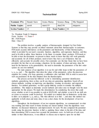
Performance Comparision of Machine Learning Algorithms
FOS Project Technical Brief
1. ENGR 132 - FOS Project Spring 2016
Technical Brief
Teammate FNs: Hannah Snow Jessica Murray Senzeyu Zhang Mia Sheppard
Purdue Logins: snowh murra119 zhan2196 shepparm
Section Number: 15 Team Number: 04
To: President Frank O. Simpson
From: Section : 15, Team 4
RE: FOS Project
Date: Class 31
The problem involves a quality analysis of thermocouples designed by First Order
Systems so that they may provide an ethical statement about their thermocouples to customers.
FOS needs accurate information on the parameters and functionality of their thermocouples,
which is provided by our team’s executive function, algorithm, and regression function, and they
need to be able to utilize these functions in the future to examine future products. FOS needs to
be able to trust the documents we present to them; needs to know that they will work generally
and accurately for all of their products; need to know they have a set of functions that run
efficiently and accounts for possible errors. Our constraints are: the time frame that we have been
provided; the fact that we are creating a functions for the analysis of clean and noisy data; the
need for the functions to be generalizable; the need to determine the parameters of the first order
system via our own methods.
The main purpose of our algorithm is to use for and while loops to find the parameters of
ts, ys, yss, and �. The algorithm then takes the values of the parameters, solves the piecewise
equation for yt using a for loop, generates a calibration plot, and finds SSE in order to assess how
well our parameters fit the data obtained from the thermocouples.
The process our team has followed so far is: determining parameter identification
methods; generalizing them so they can fit any data set; generating algorithms based off our
chosen methods; working on improving one algorithm; creating an executive and regression
function. For method generation, we had a group thinking session to consider the multiple
possibilities. This helped us determine several methods and select ones we thought were the most
appropriate for this project. We made this determination by considering the errors that could
occur, whether or not it was possible to code in MATLAB, and whether or not it fit our skill sets
as a team so everyone could be involved. We settled on a method that set limitations on the data
to allow us to pinpoint ts, ys, and yss. This then allowed us to find �, and since this method was
applicable to both clean and noisy data, it was a clear choice for the development of our two
algorithms.
Throughout the development of our two separate algorithms, we communicated on what
was working and what wasn't to better develop our chosen method. Once the algorithms were
finished, we discussed limitations and improvements for each. We also compared the parameter
results using the piecewise function to find yt, applying those values to the plot of the data, and
then determining SSE to assess how accurate the parameters were. As both sets of code were
similar in their effectiveness, it was difficult to choose one to improve upon for our final
2. ENGR 132 - FOS Project Spring 2016
Technical Brief
algorithm. Since we were going to work together to improve and develop whichever code was
chosen, we decided to simply choose one and commit to it for the rest of the FOS project.
Since the determination of which algorithm to use and develop, we have communicated
as a group to determine faults in the code, how to improve efficiency, and how to improve
accuracy in determining parameters. We’ve refined the code as we’ve progressed, making sure
each line worked in the best possible way. We’ve made sure the algorithm, regression function,
and executive function fit as an effective triad for quality analysis to complete all goals. These
goals were: identify parameters; complete a statistical analysis of �; execute regression to
complete a price analysis; determine SSE for each model. We’ve made sure our variables lined
up across functions, appropriate function calls have been made, we’ve all contributed to the
structuring and execution of the functions, and have checked that each part is working before
progressing. We’ve made sure to delegate so that everyone has had something to do the entire
process.
The first step in our algorithm is to load the data and separate it into temperature and time
variables. Then, to find ys, limits are set on the data to better evaluate it. To determine the bottom
limit, we find the minimum of the total data. To determine the top limit, we double the
minimum. To determine ys, a while loop is executed that checks for when the temperature
exceeds the limits. For this to occur, we initialize the index at 1, then after running through the
loop, we check to see if the result is accurate. We then execute another while loop that checks
subsequent data points to see if they are still between the limits. If they are, the algorithm returns
to the initial loop, and if they aren’t, then the algorithm stops running the loops.
Once the loops terminate, we set the index to index = index -1, as the function result is
one value over the desired result for ys. Then ys is produced with ys = Temp(index) and ts is
produced with ts = Time(index). To determine yss, we set new limits and initialize the index to
execute the same loop. However, instead of starting with the first data point and progressing
forward in index, the loops begins at the end of the data and progresses backwards in index. We
then produce yss with yss = Temp(index).
To determine the value of �, we execute the following calculation to find y�: y� = ys +
(.632 * (yss - ys)). From there, we set limits so that we can determine which time value
corresponds with y�. To set the upper bound we execute the following calculation: topBound =
y� + y� * .008. To set the lower bound we execute the following calculation: bottomBound = y�
- y� * .008. We then use conditional statements to determine x� so that we can then determine �
by subtracting ts from x� Finally, ys, ts, yss, and � are printed to the command window.
Table 1 displays the mean and standard deviation for � throughout the five FOS
thermocouple models. After refining the code, the � values became less varied, and the
regression plot is now exponential instead of linear. In Table 2, the r2 value is 0.9519, so it
accounts for 95% variance. This means the line represents the data well. The SSE value and SST
value from Table 2 are related to Figure 1. SSE is the sum of squared error and SST is the total
sum of squares. Figure 1 is a representation of the time constants (�) from the 100 time histories
plotted against the price of each model. As stated above, it is seen that the regression line now
accurately represents the time constants.
In a perfect experiment, the data would be clean, but the data we received is noisy, so this
is a place error occurs. This accounts for the quality of the experiments themselves. The error in
this process also occurs due to the range of the data, which means that there were instances
3. ENGR 132 - FOS Project Spring 2016
Technical Brief
where the range between two data points was quite large and exceeded the limits that we had to
set in order to determine ts, ys, and yss. At first, our parameter identification range was extremely
inaccurate and large because we had to account for such instances. It caused large SSE and SST
values, along with � values that had too much variation. After refining ranges, as well as the
regression plot, the SSE and SST values became much smaller and proved that the products were
consistent. In our first trial, the r2 value came out to be around 0.4, but with our refinements we
were able to get the r value to 0.952.
FOS can say that their products are consistent in performance, pricing and manufacturing.
They can say this and support their statement with the regression model and r2 valued. The r2
value is 0.952, so this shows that the data fits well and that it is consistent.
Niemann, H., & Miklos, R. (2014). A Simple Method for Estimation of Parameters in First
Order Systems [Abstract]. J. Phys.: Conf. Ser. Journal of Physics: Conference Series,
570(1), 012001. Retrieved March 28, 2016.
Table 1
Model
Number
τ Characteristics
SSEmod,ave
Mean Standard Deviation
FOS-1 0.189660 0.028182 2.4022
FOS-2 0.474560 0.031535 2.6576
FOS-3 0.735350 0.054435 3.3350
FOS-4 1.166220 0.067187 4.2280
FOS-5 1.688610 0.069588 4.5325
Figure 1