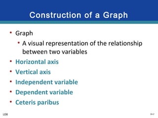
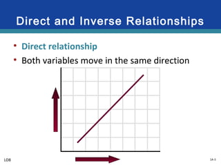
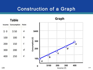
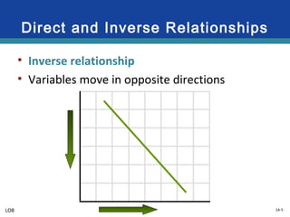
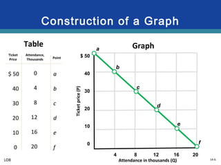
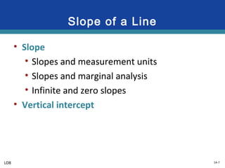
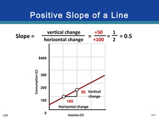
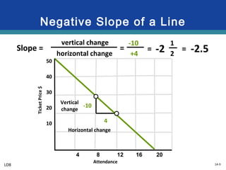
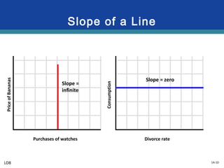
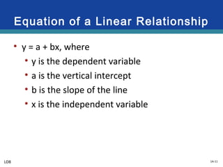
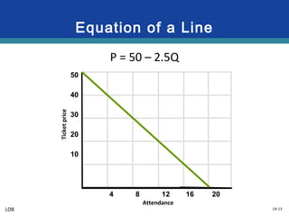
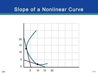
Chapter 1A
Graphs and Their Meaning
Copyright © 2015 McGraw-Hill Education. All rights reserved. No reproduction or distribution without the prior written consent of McGraw-Hill Education.
1A-2
Construction of a Graph
• Graph
• A visual representation of the relationship
between two variables
• Horizontal axis
• Vertical axis
• Independent variable
• Dependent variable
• Ceteris paribus
LO8
1A-3
Direct and Inverse Relationships
• Direct relationship
• Both variables move in the same direction
LO8
1A-4
Construction of a Graph
Table Graph
Income Consumption Point
$ 0
100
200
300
400
$ 50
100
150
200
250
a
b
c
d
e
Consumption(C)
Income (Y)
$100 200 300 400
a
b
c
d
e
$400
300
200
100
0
LO8
1A-5
Direct and Inverse Relationships
• Inverse relationship
• Variables move in opposite directions
LO8
1A-6
a
b
c
d
e
f
Construction of a Graph
Table Graph
Ticket
Price
Attendance,
Thousands Point
$ 50
40
30
20
10
0
0
4
8
12
16
20
Ticketprice(P)
Attendance in thousands (Q)
4 8 12 16 20
a
b
c
d
e
$ 50
40
30
20
10
0 f
LO8
1A-7
Slope of a Line
• Slope
• Slopes and measurement units
• Slopes and marginal analysis
• Infinite and zero slopes
• Vertical intercept
LO8
1A-8
Positive Slope of a Line
Slope =
vertical change
horizontal change
+50
+100
= 0.5==
1
2
LO8
Consumption(C)
Income (Y)
$400
300
200
100
0
50
100
Vertical
change
Horizontal change
1A-9
Negative Slope of a Line
Slope =
vertical change
horizontal change
=
-10
+4
=
1
2-2 = -2.5
50
40
30
20
10
4 8 12 16 20
-10
4
Horizontal change
Vertical
change
TicketPrice$
Attendance
LO8
1A-10
Slope of a Line
PriceofBananas
Consumption
Purchases of watches Divorce rate
Slope =
infinite
Slope = zero
LO8
1A-11
Equation of a Linear Relationship
• y = a + bx, where
• y is the dependent variable
• a is the vertical intercept
• b is the slope of the line
• x is the independent variable
LO8
1A-12
Equation of a Line
Consumption(C)
Income (Y)
$100 200 300 400
$400
300
200
100
0
Y = 50 + .5C
LO8
1A-13
Equation of a Line
P = 50 – 2.5Q
50
40
30
20
10
4 8 12 16 20
Ticketprice
Attendance
LO8
1A-14
Slope of a Nonlinear Curve
• Slope always changes
• Use a line tangent to the curve to find slope at
that point
LO8
1A-15
Slope of a Nonlinear Curve
20
15
10
5
0
5 10 15 20LO8

Econ706 chapter001a

  • 1.
    Chapter 1A Graphs andTheir Meaning Copyright © 2015 McGraw-Hill Education. All rights reserved. No reproduction or distribution without the prior written consent of McGraw-Hill Education.
  • 2.
    1A-2 Construction of aGraph • Graph • A visual representation of the relationship between two variables • Horizontal axis • Vertical axis • Independent variable • Dependent variable • Ceteris paribus LO8
  • 3.
    1A-3 Direct and InverseRelationships • Direct relationship • Both variables move in the same direction LO8
  • 4.
    1A-4 Construction of aGraph Table Graph Income Consumption Point $ 0 100 200 300 400 $ 50 100 150 200 250 a b c d e Consumption(C) Income (Y) $100 200 300 400 a b c d e $400 300 200 100 0 LO8
  • 5.
    1A-5 Direct and InverseRelationships • Inverse relationship • Variables move in opposite directions LO8
  • 6.
    1A-6 a b c d e f Construction of aGraph Table Graph Ticket Price Attendance, Thousands Point $ 50 40 30 20 10 0 0 4 8 12 16 20 Ticketprice(P) Attendance in thousands (Q) 4 8 12 16 20 a b c d e $ 50 40 30 20 10 0 f LO8
  • 7.
    1A-7 Slope of aLine • Slope • Slopes and measurement units • Slopes and marginal analysis • Infinite and zero slopes • Vertical intercept LO8
  • 8.
    1A-8 Positive Slope ofa Line Slope = vertical change horizontal change +50 +100 = 0.5== 1 2 LO8 Consumption(C) Income (Y) $400 300 200 100 0 50 100 Vertical change Horizontal change
  • 9.
    1A-9 Negative Slope ofa Line Slope = vertical change horizontal change = -10 +4 = 1 2-2 = -2.5 50 40 30 20 10 4 8 12 16 20 -10 4 Horizontal change Vertical change TicketPrice$ Attendance LO8
  • 10.
    1A-10 Slope of aLine PriceofBananas Consumption Purchases of watches Divorce rate Slope = infinite Slope = zero LO8
  • 11.
    1A-11 Equation of aLinear Relationship • y = a + bx, where • y is the dependent variable • a is the vertical intercept • b is the slope of the line • x is the independent variable LO8
  • 12.
    1A-12 Equation of aLine Consumption(C) Income (Y) $100 200 300 400 $400 300 200 100 0 Y = 50 + .5C LO8
  • 13.
    1A-13 Equation of aLine P = 50 – 2.5Q 50 40 30 20 10 4 8 12 16 20 Ticketprice Attendance LO8
  • 14.
    1A-14 Slope of aNonlinear Curve • Slope always changes • Use a line tangent to the curve to find slope at that point LO8
  • 15.
    1A-15 Slope of aNonlinear Curve 20 15 10 5 0 5 10 15 20LO8

Editor's Notes

  • #2 This appendix helps in understanding graphs, curves, and slopes as they relate to economics. It demonstrates how relationships between variables can be examined and how an equation that expresses that relationship can be derived.
  • #3 The two dimensional graphs used in this textbook consist of a horizontal axis and a vertical axis. The point where the two meet is called the origin. As one moves away from the origin either up or to the right, the plotted values increase. Often the independent variable which is the variable that changes first, is placed on the horizontal axis and the dependent variable which is the variable that changes in response to the first variable changing, is placed on the vertical axis. However, in economics it is customary to always place price or cost data on the vertical axis even if it is the independent variable. Economist invoke the ceteris paribus assumption in economics in order to be able to analyze just the two variables that are labeled on the axis. Ceteris paribus means to hold other things equal or constant and assumes that the only changes in the model are brought about by the dependent variable changing in response to the change in the independent variable.
  • #4 Direct or positive relationships occur as the two variables change in the same direction. In other words, when the independent variable increases (decreases), the dependent variable also increases (decreases). This graphs as an upsloping line.
  • #5 Each pair of values in the table represents one point on the graph. This data represents variables that are positively or directly related, such as income and consumption, which will graph as an upsloping line.
  • #6 Inverse or negative relationships are those where the two variables move in opposite directions. So when the independent variable increases (decreases), the dependent variable decreases (increases). An inverse relationship graphs as a downsloping line.
  • #7 Each pair of values in the table represents one point on the graph. This data represents variables that are negatively or inversely related, such as ticket price and attendance at basketball games, which will graph as a downsloping line.
  • #8 The slope of a line can vary based on the units that are used to measure the slope. If in the ticket price and attendance example, if the number 4000 had been used instead of 4 for the horizontal change, the slope would have been -0.0025 instead of -2.5. Slope is also important in economics when analyzing marginal changes. In the income example, a slope of 0.5 means that an increase of $1 in income will result in a $.50 increase in consumption spending. If there is no relationship between the two variables, the line will graph as a vertical line parallel to the vertical axis which reflects an infinite slope or it will graph as a horizontal line that is parallel to the horizontal axis which would exhibit a slope of zero. The vertical intercept is the point where the line meets the vertical axis.
  • #9 As the independent variable, income, increases, the dependent variable, consumption, increases; this results in a positively sloped line.
  • #10 As the independent variable, ticket price increases, attendance decreases. Here the variables are moving in opposite directions illustrating a negative slope. Note: though generally the independent variable is placed on the horizontal axis, when price is one of the variables, in economics it is customary to always place it on the vertical axis.
  • #11 The graphs above show that the variables are unrelated. No matter what the price of bananas might be, the number of watches purchased remains the same. This is because the price of bananas does not affect the number of watches purchased. There is no relationship between consumption and the divorce rate. Consumption remains the same no matter how high or low the divorce rate is.
  • #12 This is the general equation of a line and expresses the relationship between the two variables y and x. If you know the slope and the vertical intercept, you can solve for y or x.
  • #13 We calculated the slope of this line earlier, and we found that the slope is +.5. We can see from the graph that the vertical intercept is 50. Therefore the equation of this line is: Y (income) = 50 (vertical intercept) + .5C (where .5 is the slope and C is the consumption).
  • #14 We calculated the slope of this line earlier, and we found that the slope is -2.5. We can see from the graph that the vertical intercept is 50. Therefore the equation of this line is: P (price) = 50 (vertical intercept) - 2.5Q (where -2.5 is the slope and Q is the quantity). In this case, the slope is being subtracted because the slope is negative.
  • #15 When calculating the slope of a nonlinear curve, the slope is always changing. This means the slope will be different at every point on the curve. In this case to find the slope, you must draw a line tangent to the curve and calculate the slope of the line by finding the change between two points along the tangent line.
  • #16 The slopes of a nonlinear curve will change along the curve. Here, the slope at these two points on the curve will be different from each other. To find the slope of a nonlinear curve, draw a straight line tangent to the curve and find the slope of that line by dividing the vertical change by the horizontal change of that line.