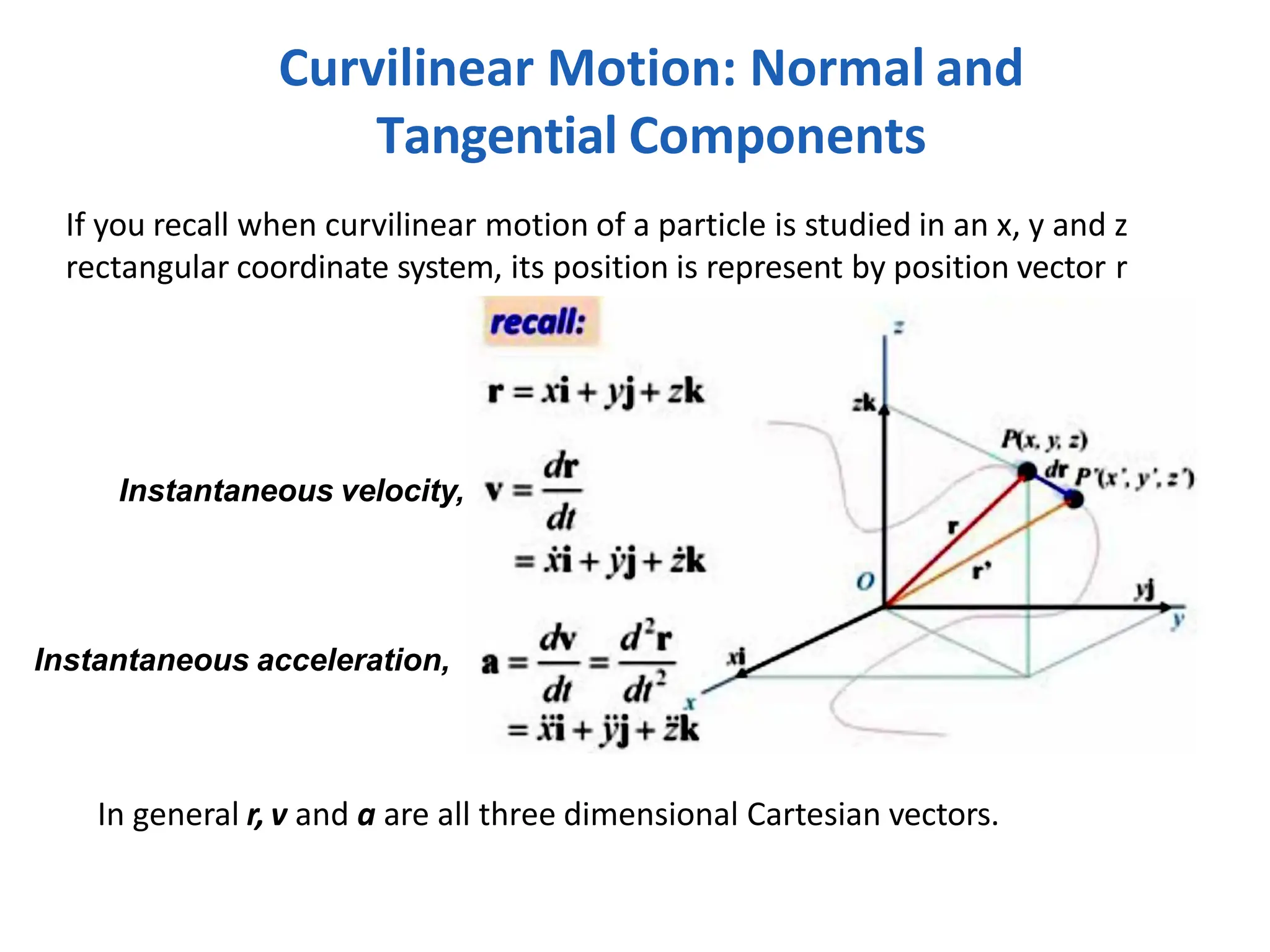
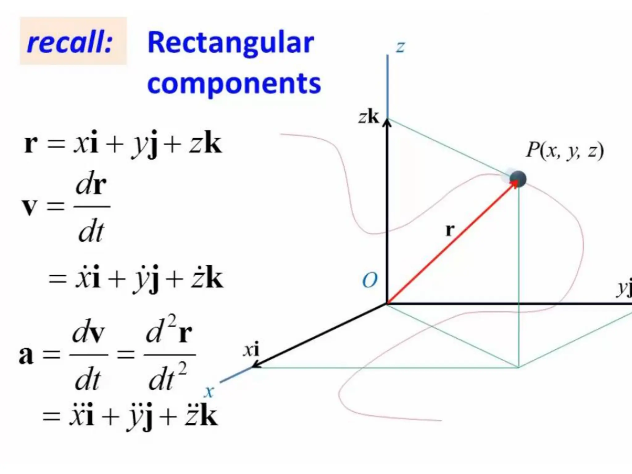
Dynamics Lecture No 5.pdf mechanical engineering

If you recall when curvilinear motion of a particle is studied in an x, y and z
rectangular coordinate system, its position is represent by position vector r
In general r, v and a are all three dimensional Cartesian vectors.
Curvilinear Motion: Normal and
Tangential Components
Instantaneous velocity,
Instantaneous acceleration,

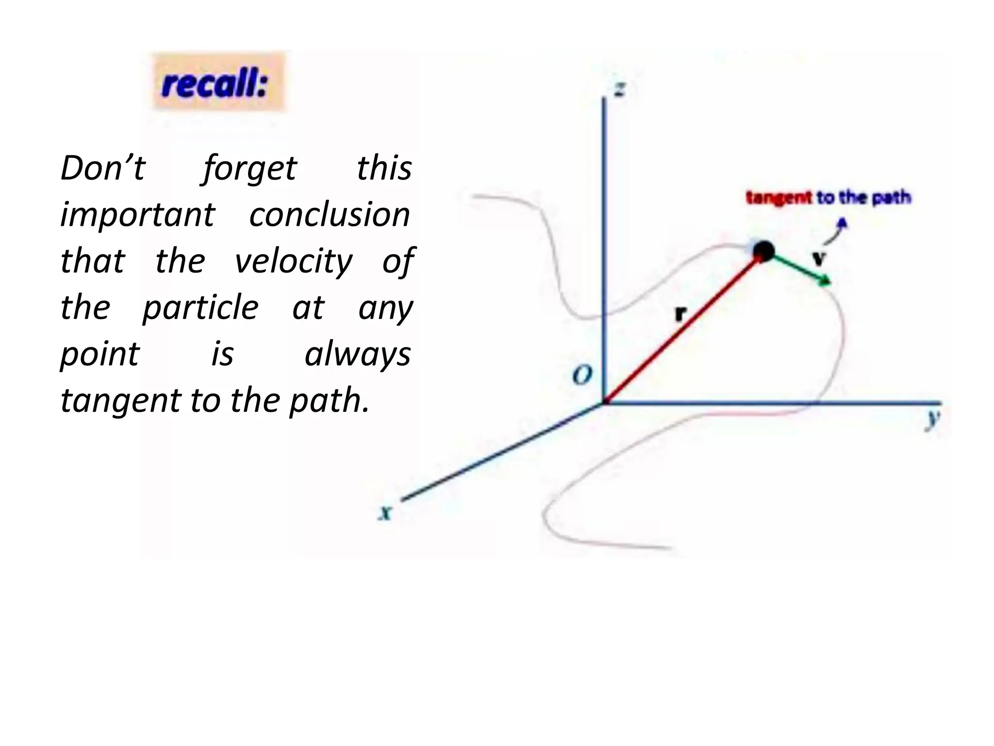
Don’t forget this
important conclusion
the velocity of
any
that
the
point
particle at
is always
tangent to the path.

It can be divided into small
segments of curves with equal
lengths.
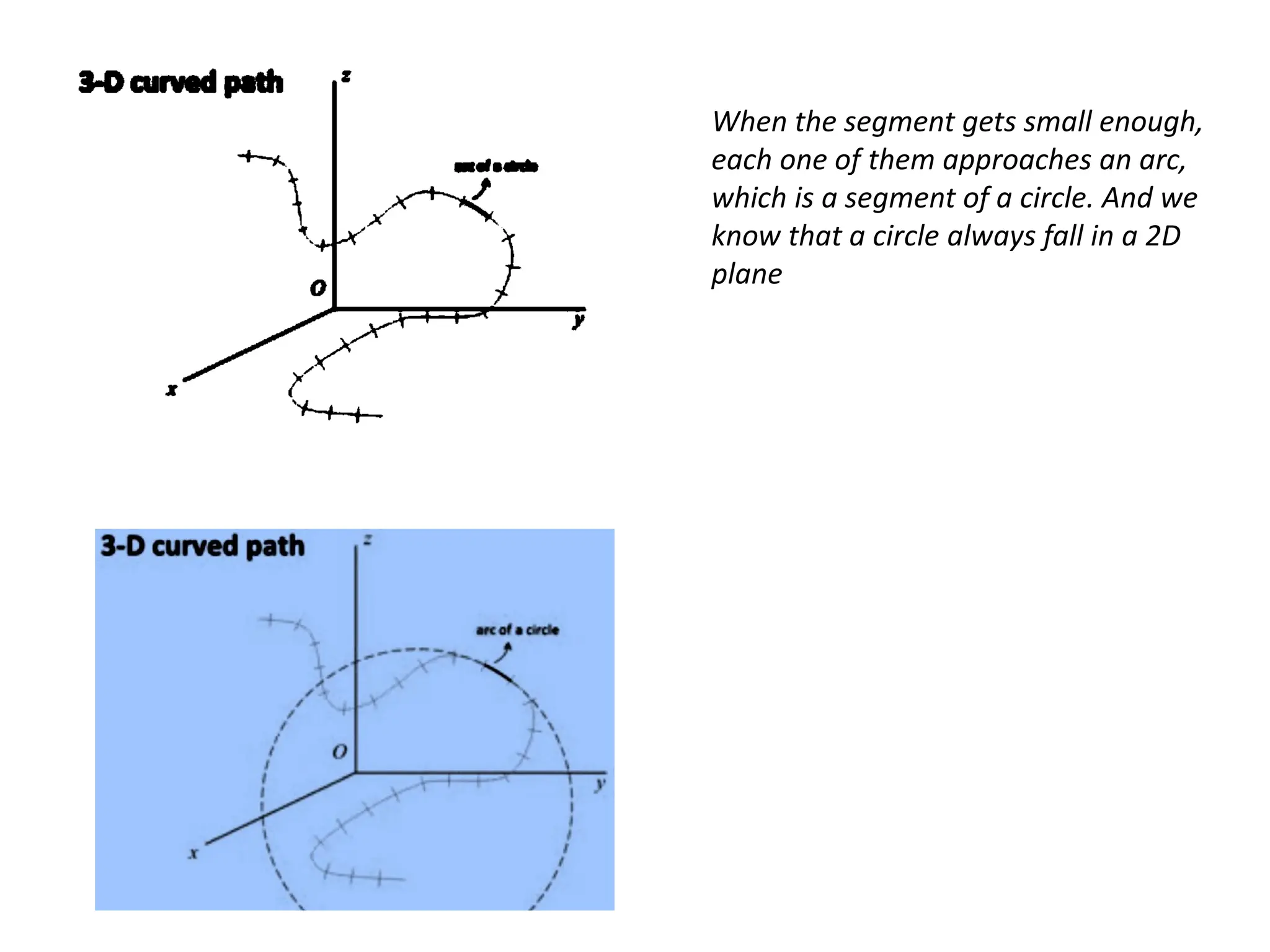
Now lets look at this 3D curve path.

When the segment gets small enough,
each one of them approaches an arc,
which is a segment of a circle. And we
know that a circle always fall in a 2D
plane

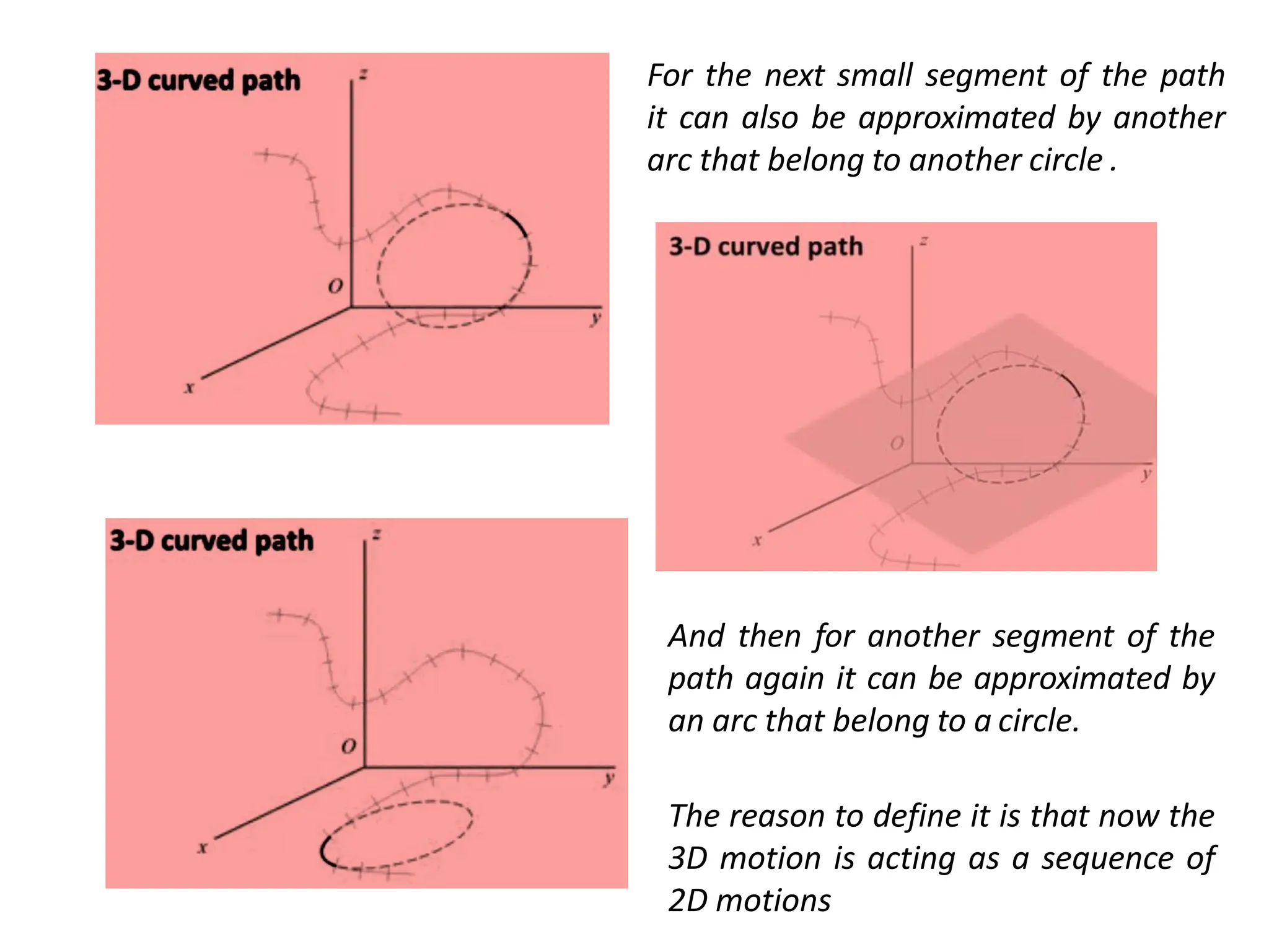
For the next small segment of the path
it can also be approximated by another
arc that belong to another circle .
And then for another segment of the
path again it can be approximated by
an arc that belong to a circle.
The reason to define it is that now the
3D motion is acting as a sequence of
2D motions

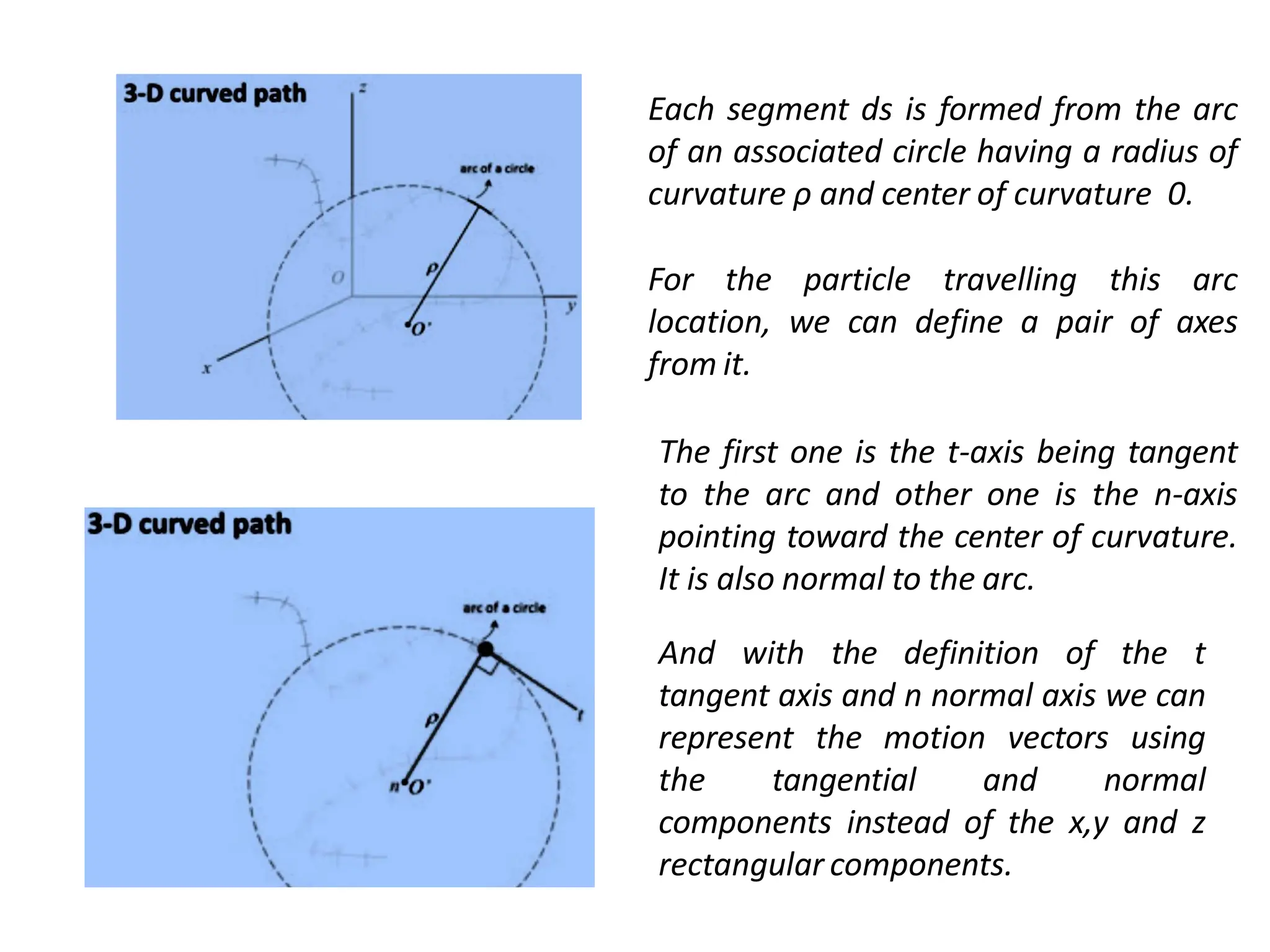
Each segment ds is formed from the arc
of an associated circle having a radius of
curvature ρ and center of curvature 0.
For the particle travelling this arc
location, we can define a pair of axes
from it.
The first one is the t-axis being tangent
to the arc and other one is the n-axis
pointing toward the center of curvature.
It is also normal to the arc.
And with the definition of the t
tangent axis and n normal axis we can
represent the motion vectors using
the tangential and normal
components instead of the x,y and z
rectangular components.

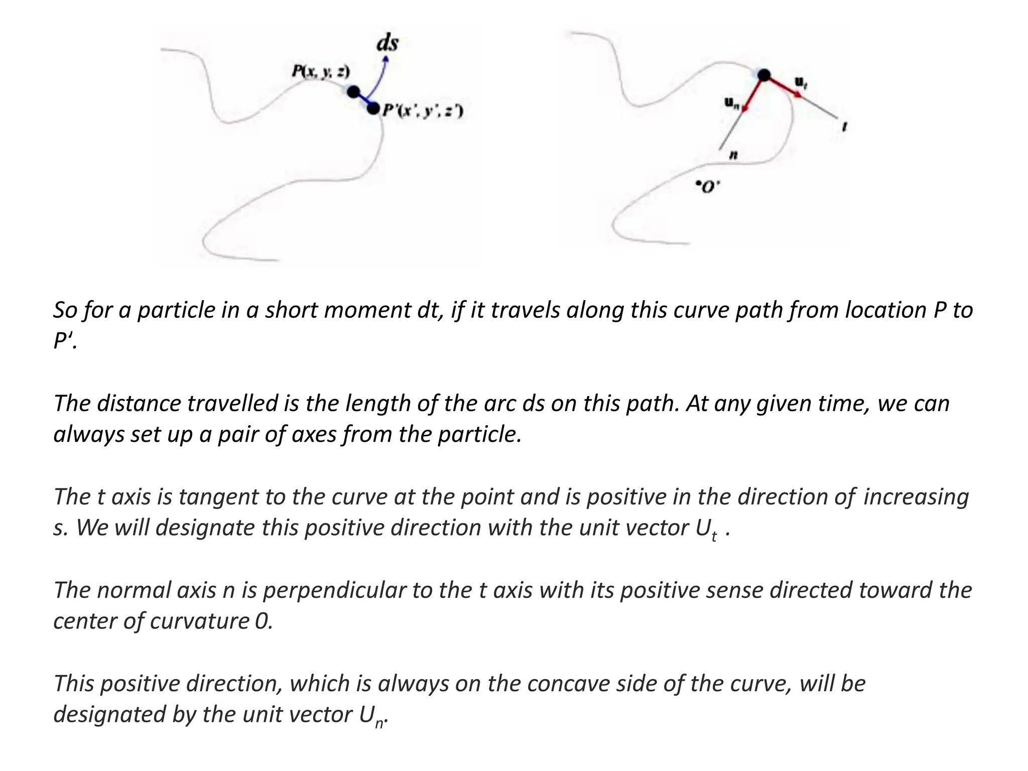
So for a particle in a short moment dt, if it travels along this curve path from location P to
Pʹ.
The distance travelled is the length of the arc ds on this path. At any given time, we can
always set up a pair of axes from the particle.
The t axis is tangent to the curve at the point and is positive in the direction of increasing
s. We will designate this positive direction with the unit vector Ut .
The normal axis n is perpendicular to the t axis with its positive sense directed toward the
center of curvature 0.
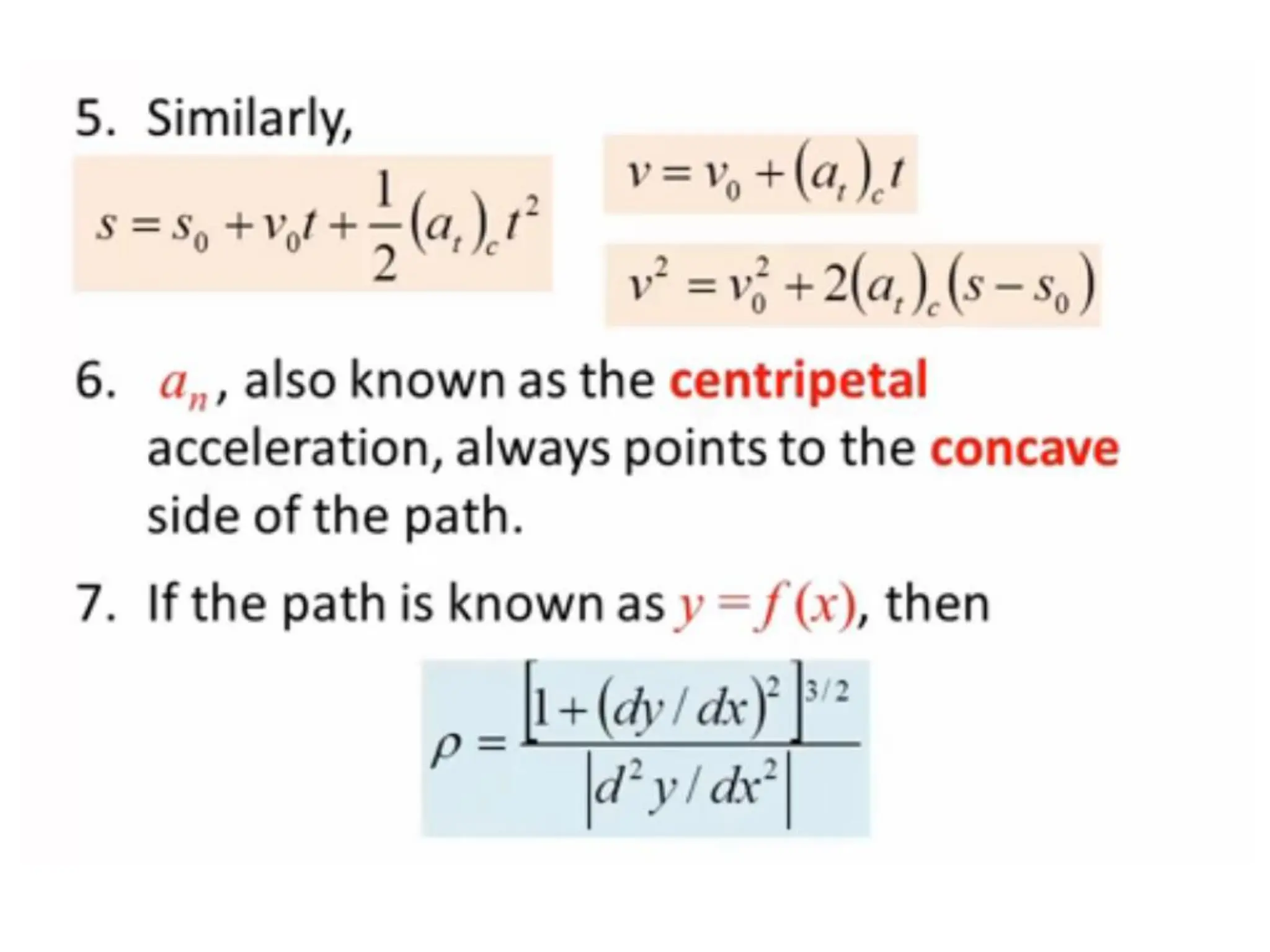
This positive direction, which is always on the concave side of the curve, will be
designated by the unit vector Un.


 s
ds
dt
v 
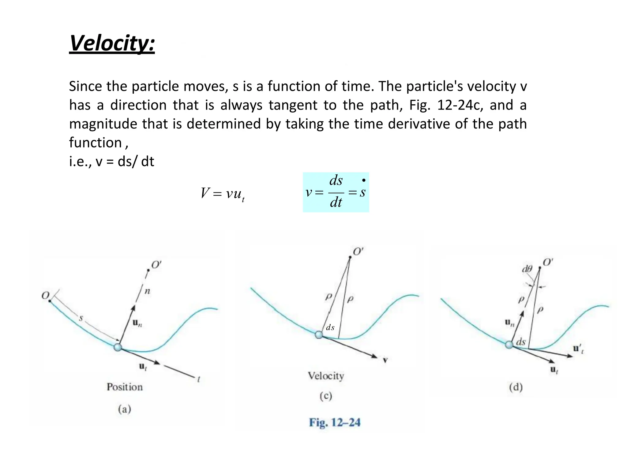
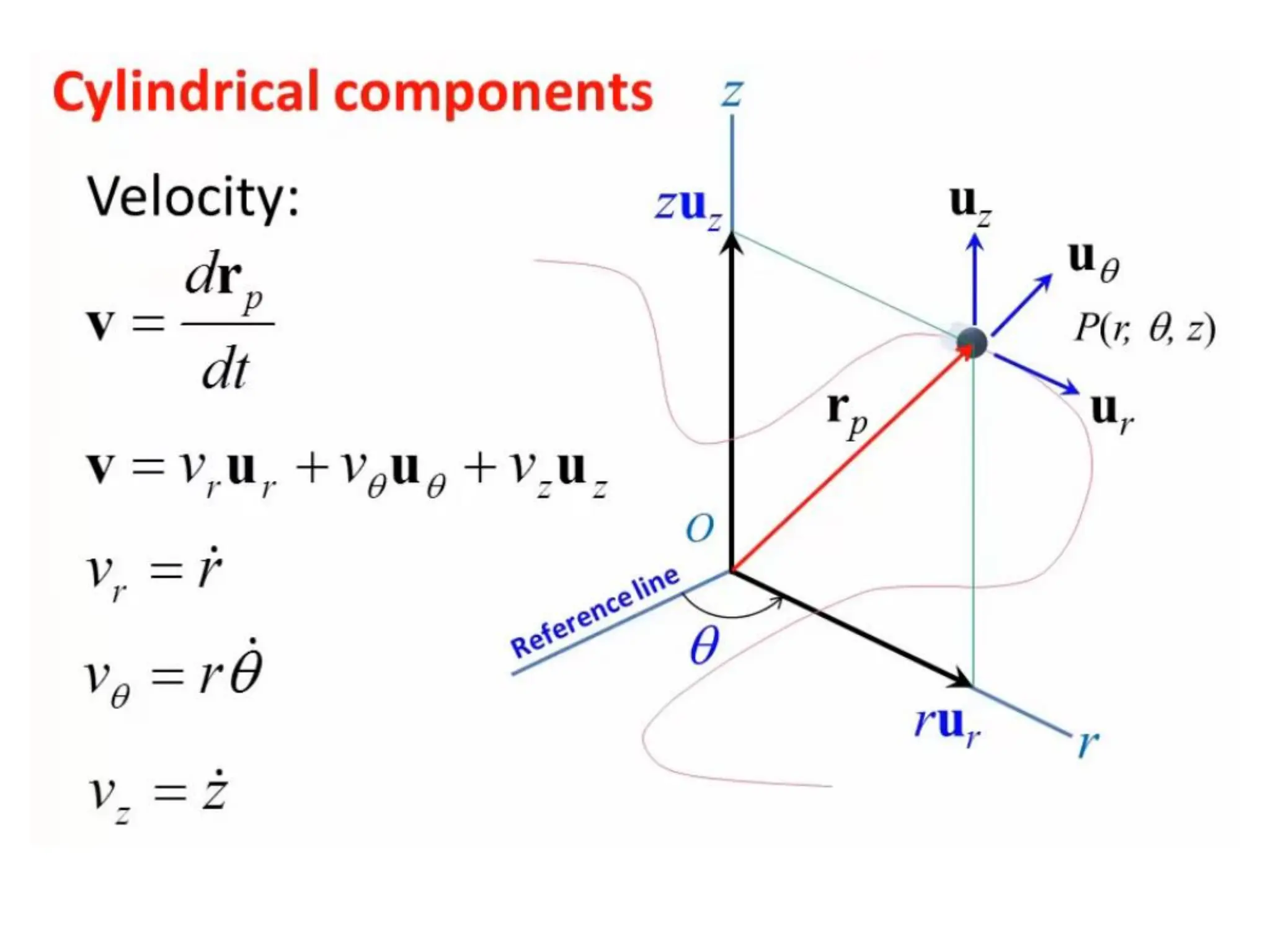
Velocity:
Since the particle moves, s is a function of time. The particle's velocity v
has a direction that is always tangent to the path, Fig. 12-24c, and a
magnitude that is determined by taking the time derivative of the path
function ,
i.e., v = ds/ dt
t
V  vu
ds

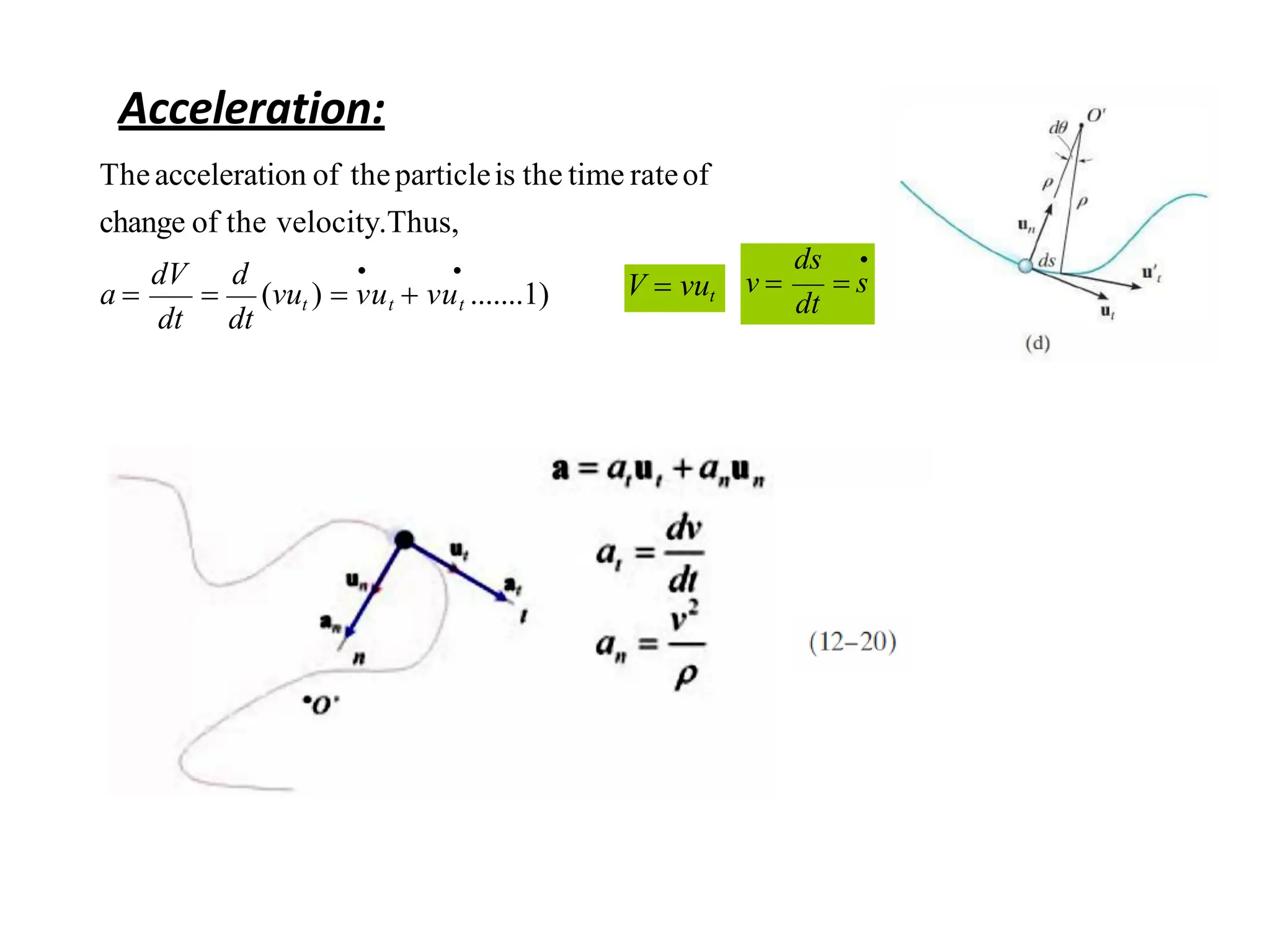
Theacceleration of theparticleis the time rateof
change of the velocity.Thus,
 
 (vut )  vut  vut .......1)
dt dt
dV d
a  V  vut

 s
ds
dt
v 
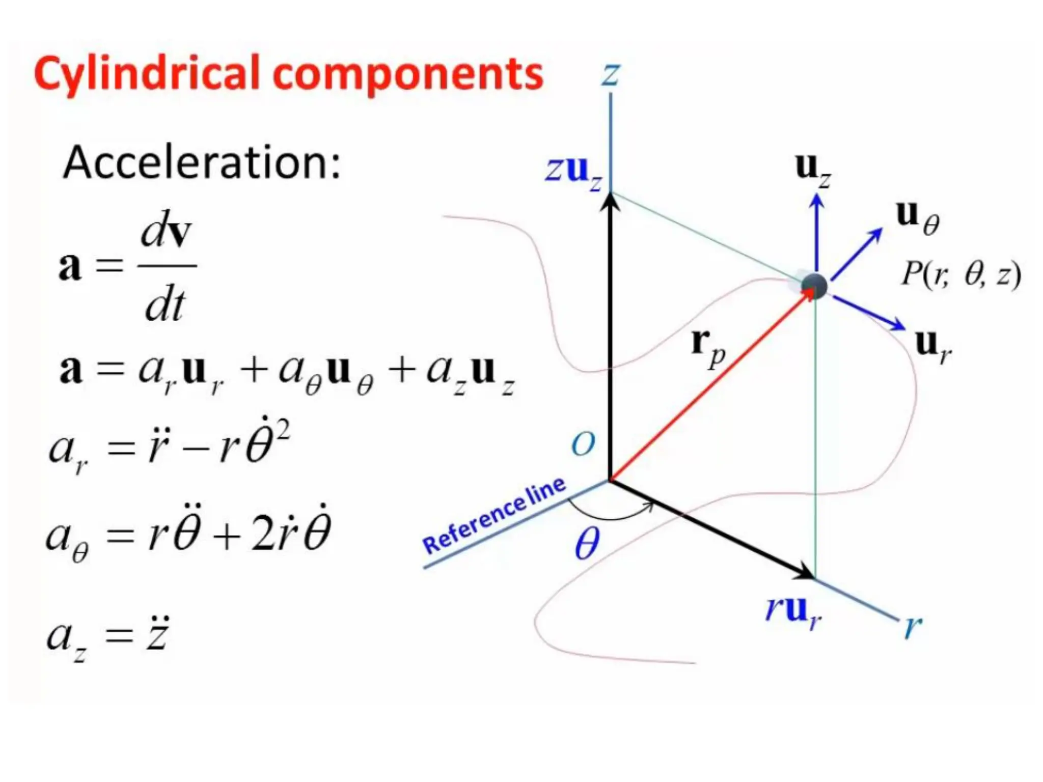
Acceleration:

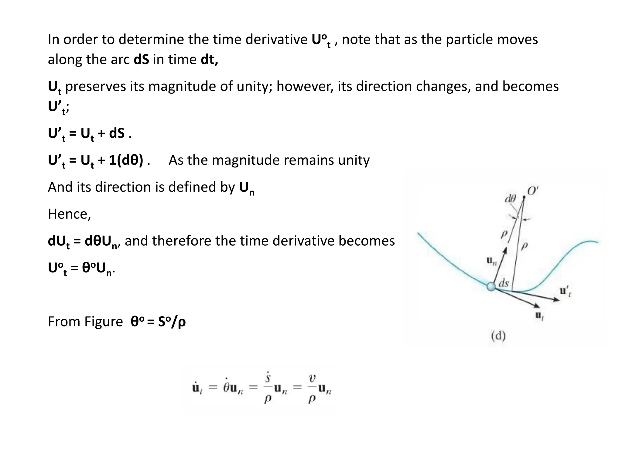
In order to determine the time derivative Uo
t , note that as the particle moves
along the arc dS in time dt,
Ut preserves its magnitude of unity; however, its direction changes, and becomes
U’t;
U’t = Ut + dS .
U’t = Ut + 1(dθ) . As the magnitude remains unity
And its direction is defined by Un
Hence,
dUt = dθUn, and therefore the time derivative becomes
Uo
t = θoUn.
From Figure θo = So/ρ

Two Special Cases of acceleration

Curvilinear Motion: Polar Coordinates
er

e
Transverse: Situated or lying across; crosswise.

Curvilinear Motion: Polar Coordinates

Assignment :
Solve this problem and plot curve between x and y for 0 < t < 5 sec

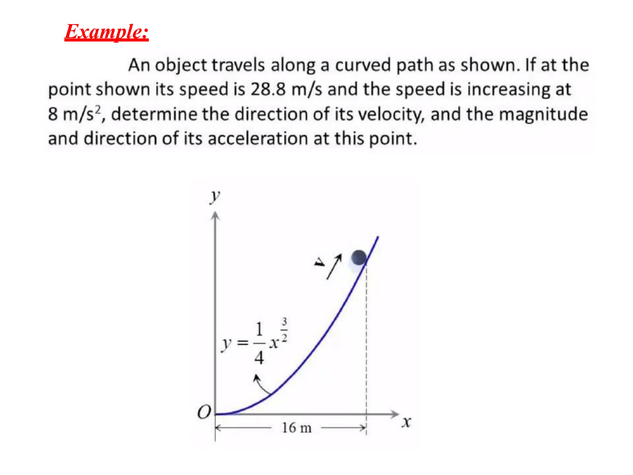
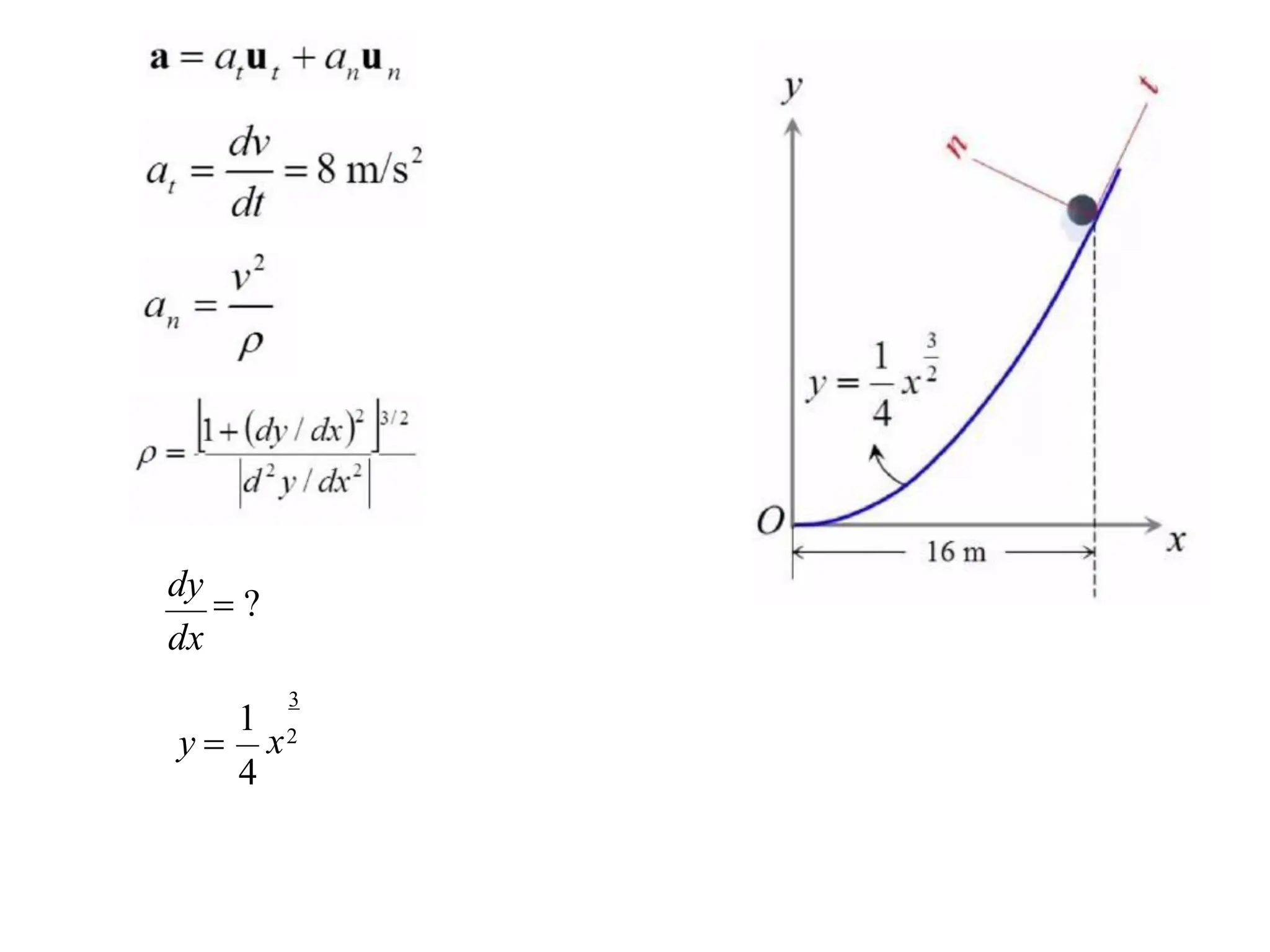
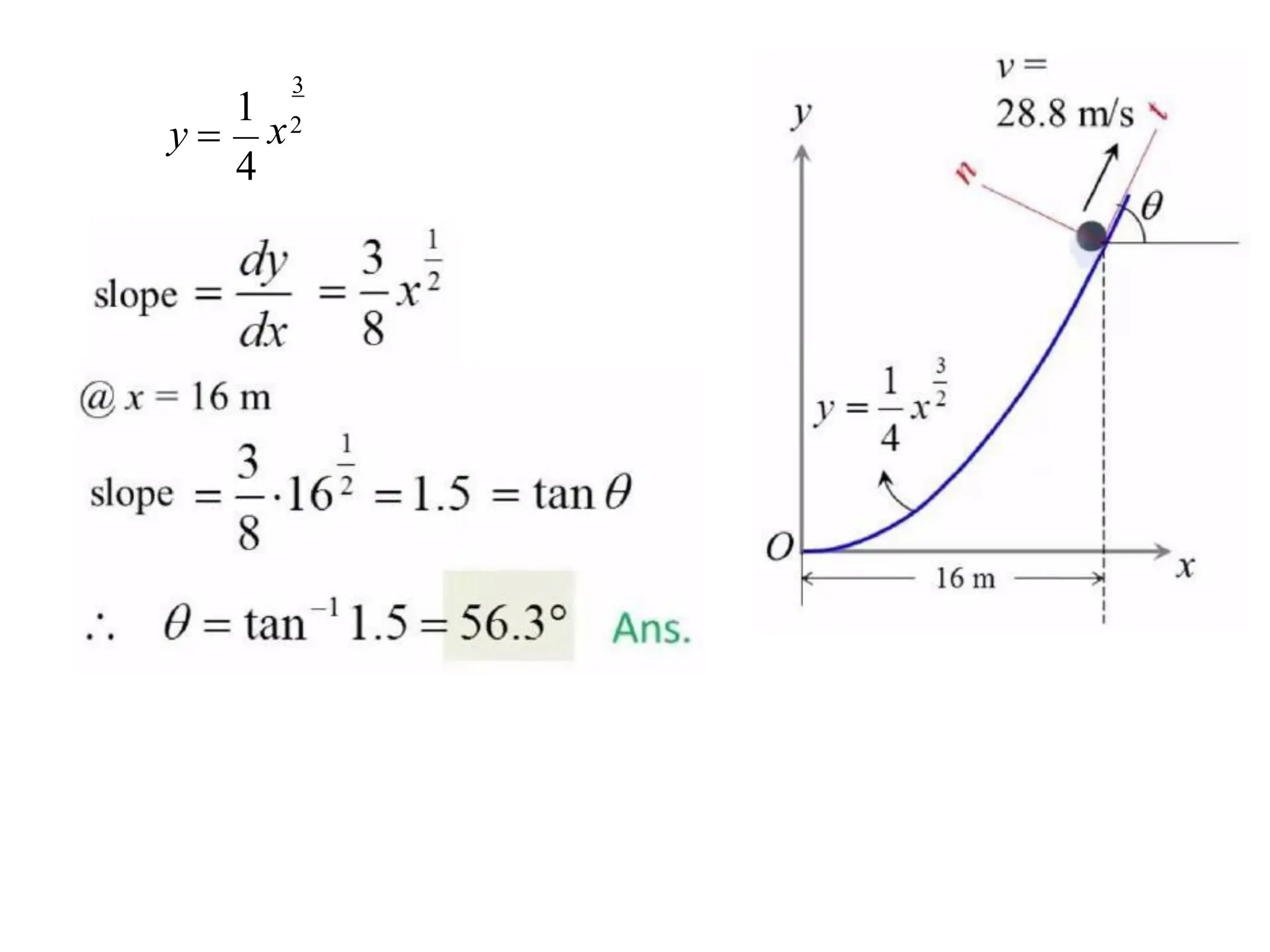
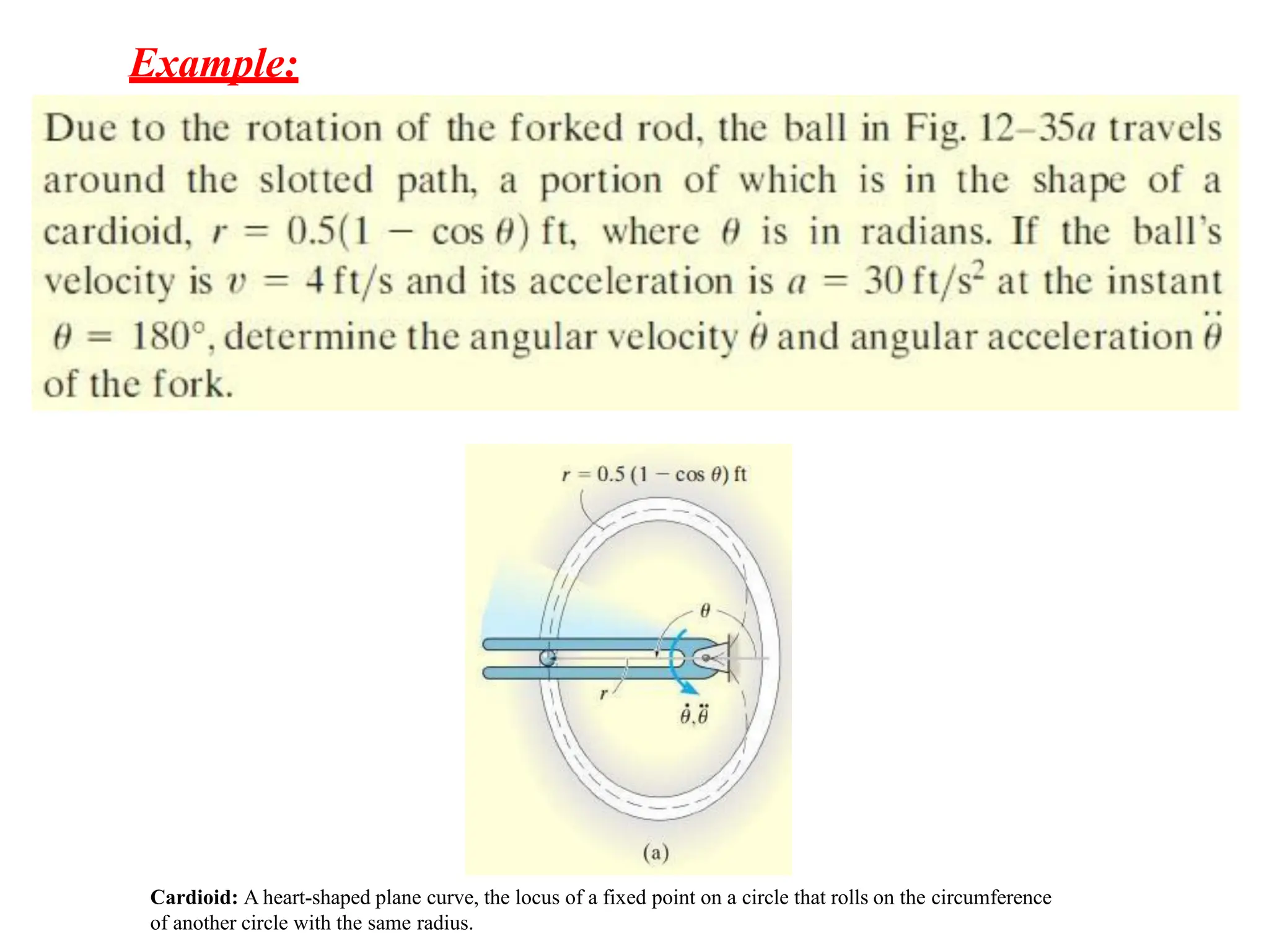
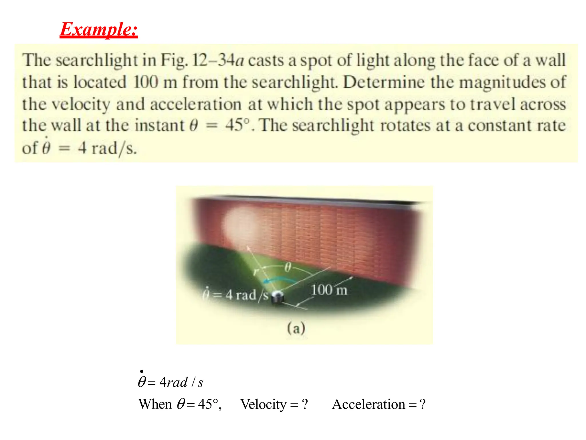
Example:
Cardioid: A heart-shaped plane curve, the locus of a fixed point on a circle that rolls on the circumference
of another circle with the same radius.

Cos180 1
Sin180 0


s2
  180
  ?
  ?
a  30
ft
r  0.5(1cos)
v  4
ft
s

Example:
Acceleration  ?
Velocity  ?

  4rad / s
When   45,

Hypotenuse r
Base

100
cos 
100m
r 90


Problem Sheet
RC Hibbler
Normal-Tangential Coordinate System
12-106; 12-117; 12-118; 12-119; 12-124; 12-125;
12-130; 12-135
Radial-Transverse Coordinate System
12-145; 12-150; 12-152; 12-154; 12-164; 12-166;
12-168; 12-169; 12-170; 12-171
JL Meriam
Normal and Tengential:
2/97,98, 99,100,101,103, 104,107, 108,112,116,122,
Polar Coordiantes:
2/131,132,134,136,137,139,142,145, 154, 168

After solving this problem and plot curve between x and y for 0 < t < 5 sec in MS-Excel

Dynamics Lecture No 5.pdf mechanical engineering

More Related Content

Similar to Dynamics Lecture No 5.pdf mechanical engineering

Recently uploaded

Dynamics Lecture No 5.pdf mechanical engineering