Download to read offline
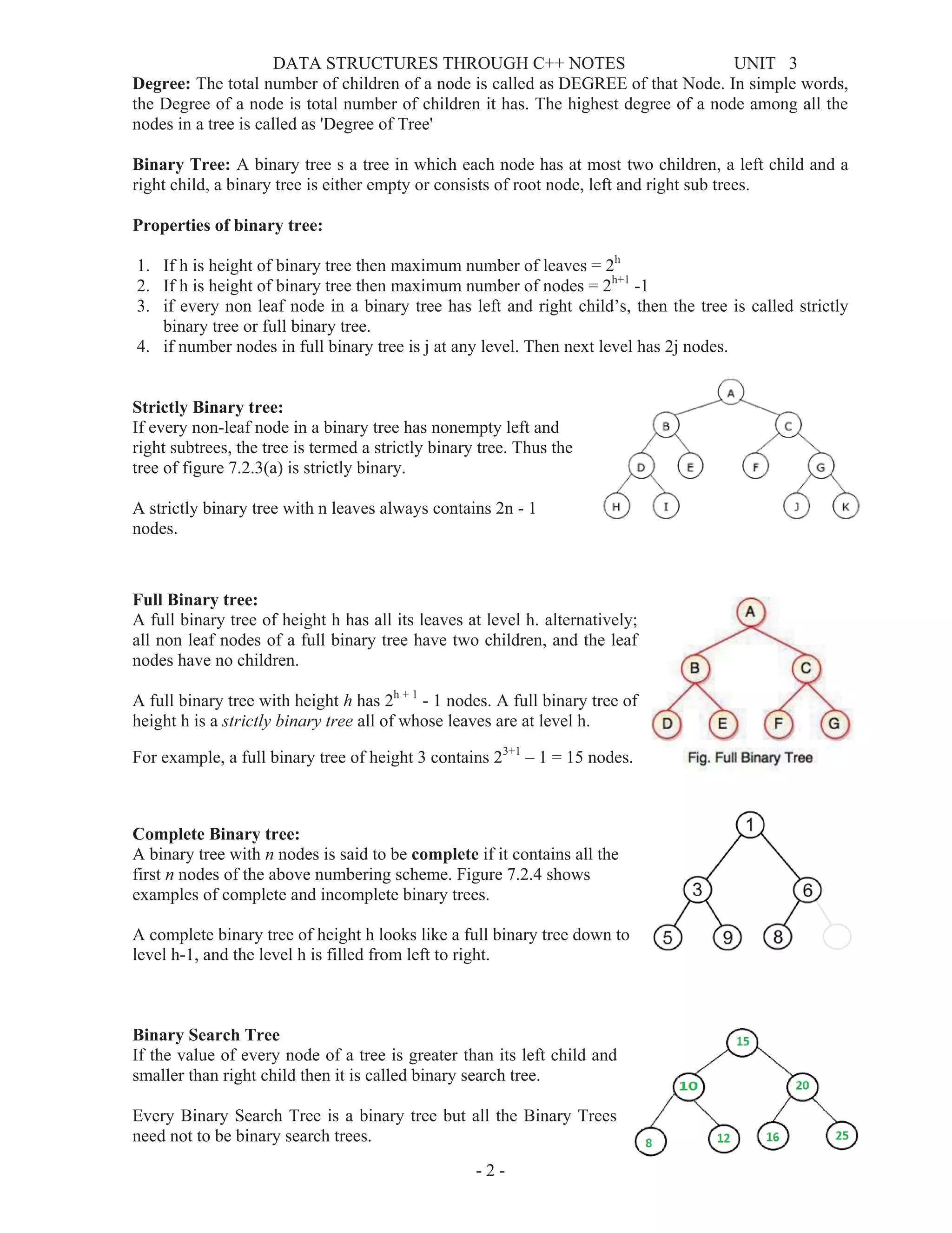
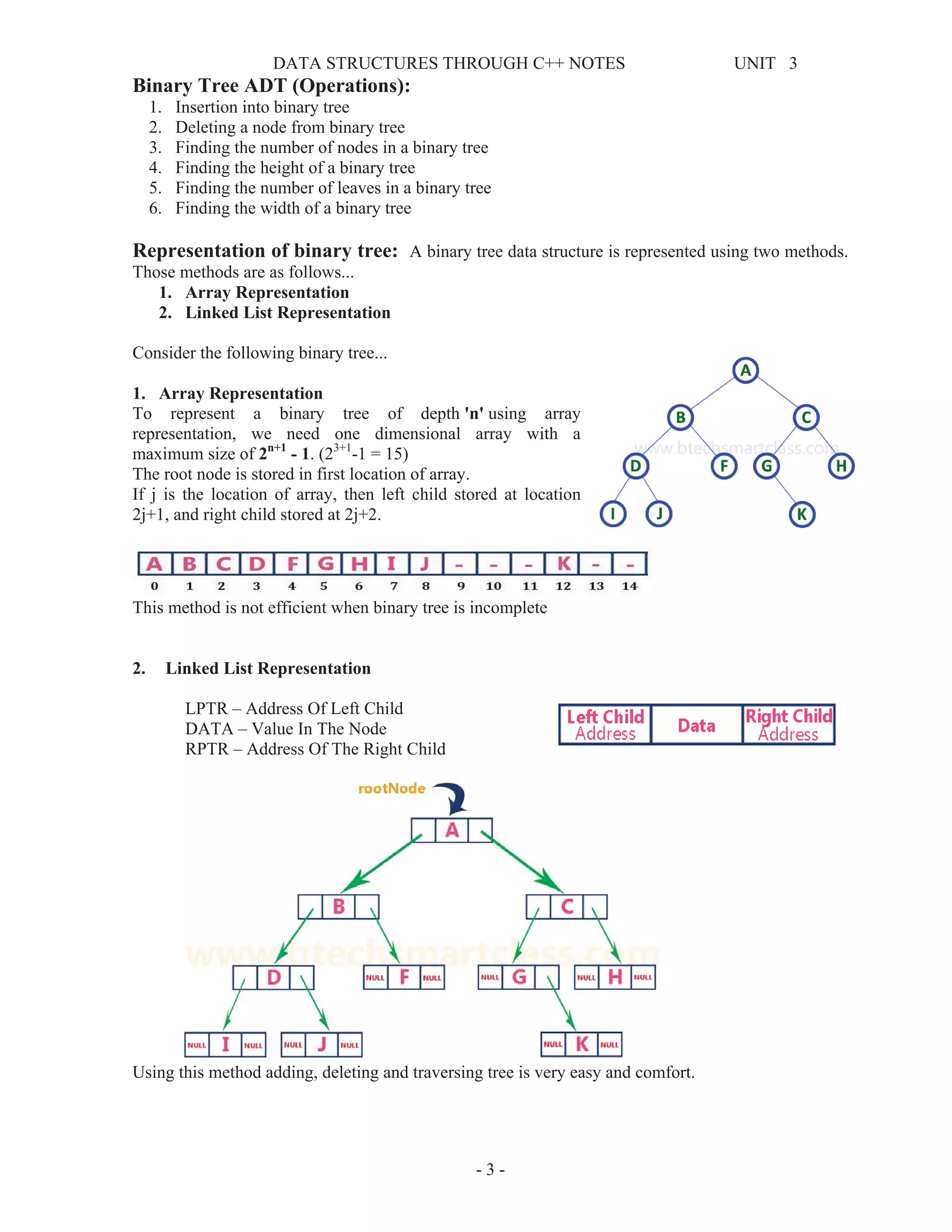
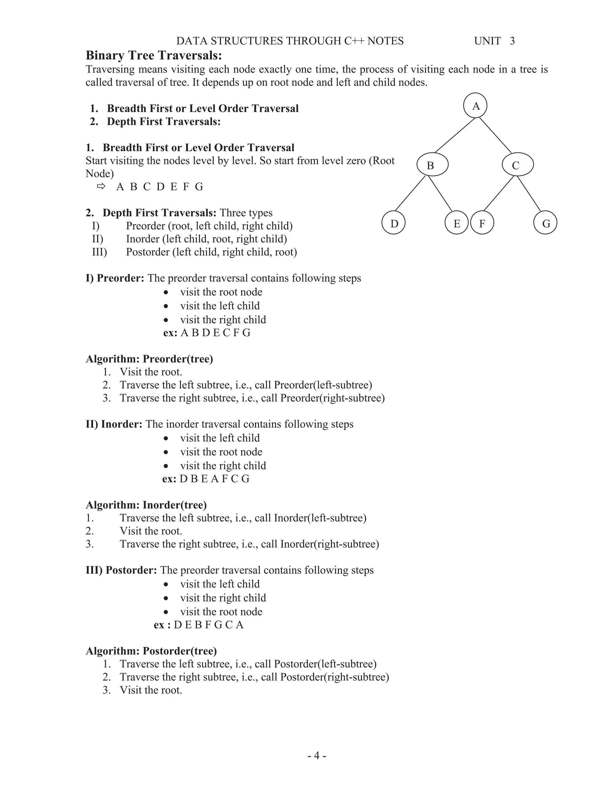
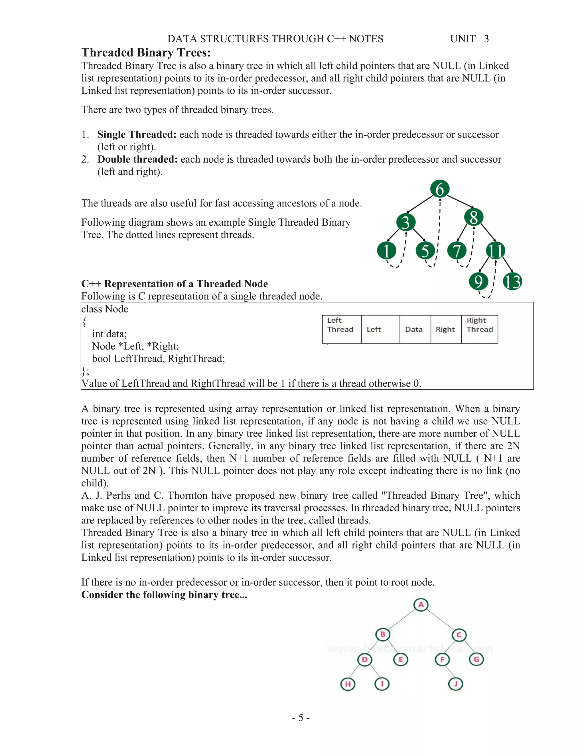
![DATA STRUCTURES THROUGH C++ NOTES UNIT 3
- 21 -
B - Trees
In a binary search tree, AVL Tree, Red-Black tree etc., every node can have only one value (key) and
maximum of two children but there is another type of search tree called B-Tree in which a node can
store more than one value (key) and it can have more than two children. B-Tree was developed in the
year of 1972 by Bayer and McCreight with the name Height Balanced m-way Search Tree. Later it
was named as B-Tree.
B-Tree can be defined as follows...
B-Tree is a self-balanced search tree with multiple keys in every node and more than two children for
every node.
Here, number of keys in a node and number of children for a node is depend on the order of the B-
Tree. Every B-Tree has order.
B-Tree of Order m has the following properties...
• Property #1 - All the leaf nodes must be at same level.
• Property #2 - All nodes except root must have at least [m/2]-1 keys and maximum of m-1
keys.
• Property #3 - All non leaf nodes except root (i.e. all internal nodes) must have at least m/2
children.
• Property #4 - If the root node is a non leaf node, then it must have at least 2 children.
• Property #5 - A non leaf node with n-1 keys must have n number of children.
• Property #6 - All the key values within a node must be in Ascending Order.
For example, B-Tree of Order 4 contains maximum 3 key values in a node and maximum 4 children
for a node.
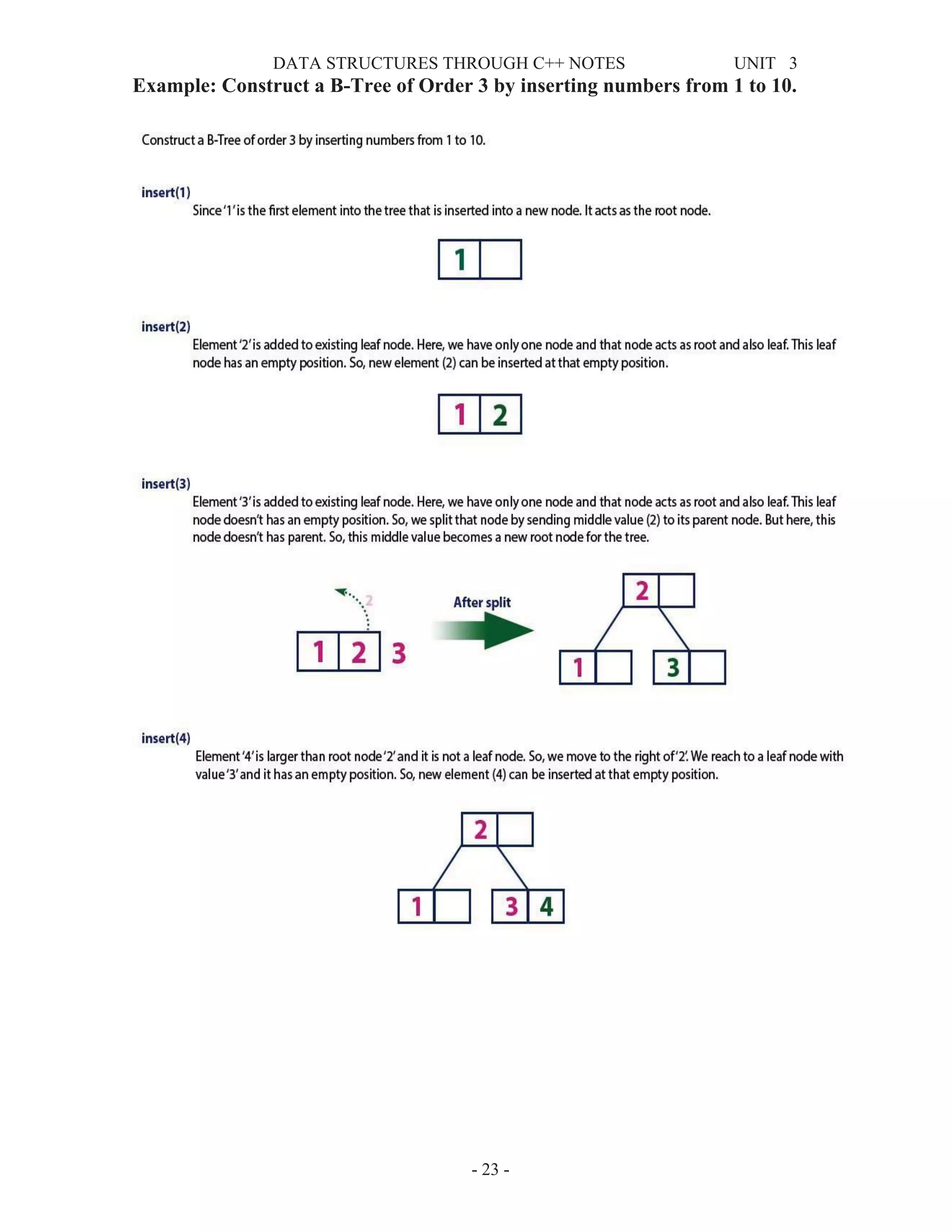
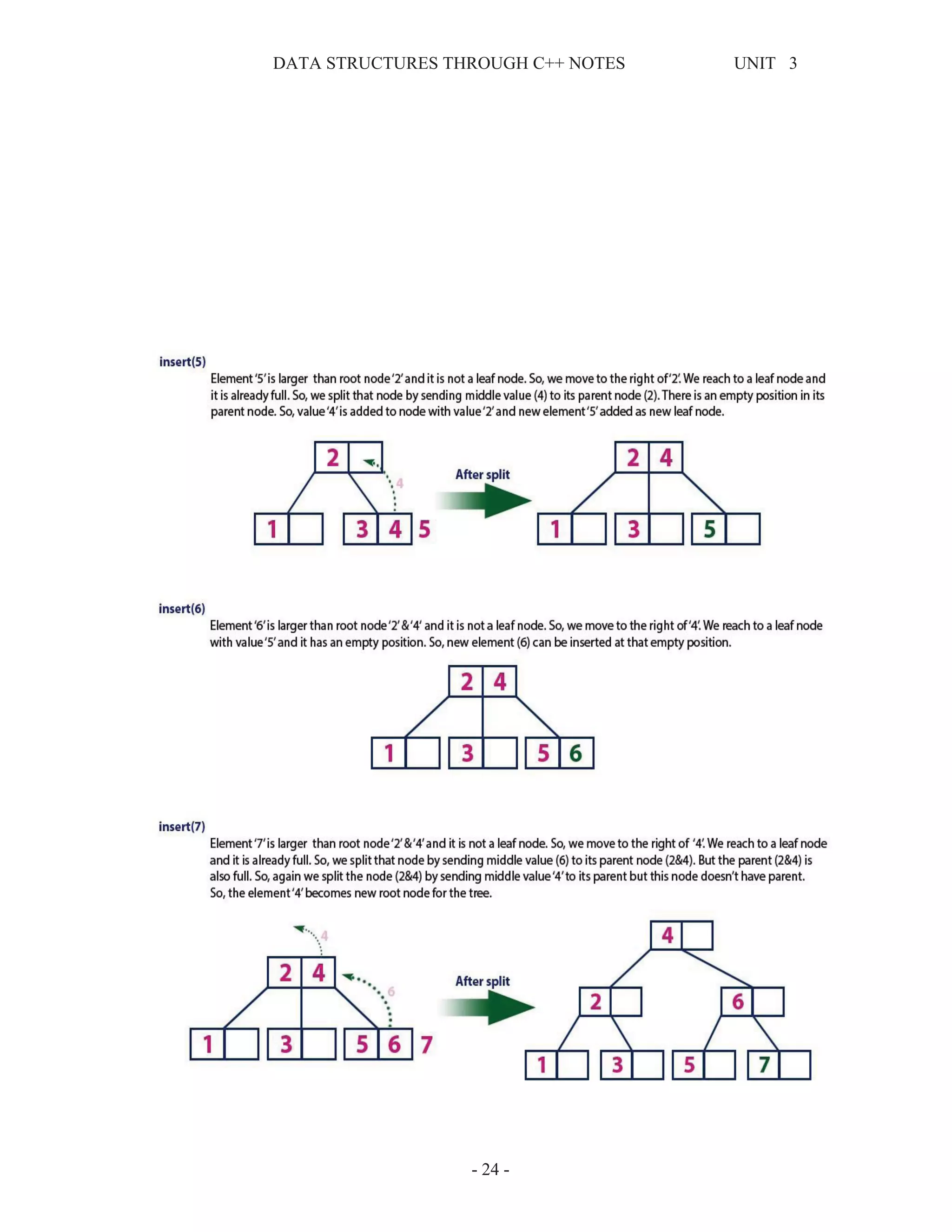
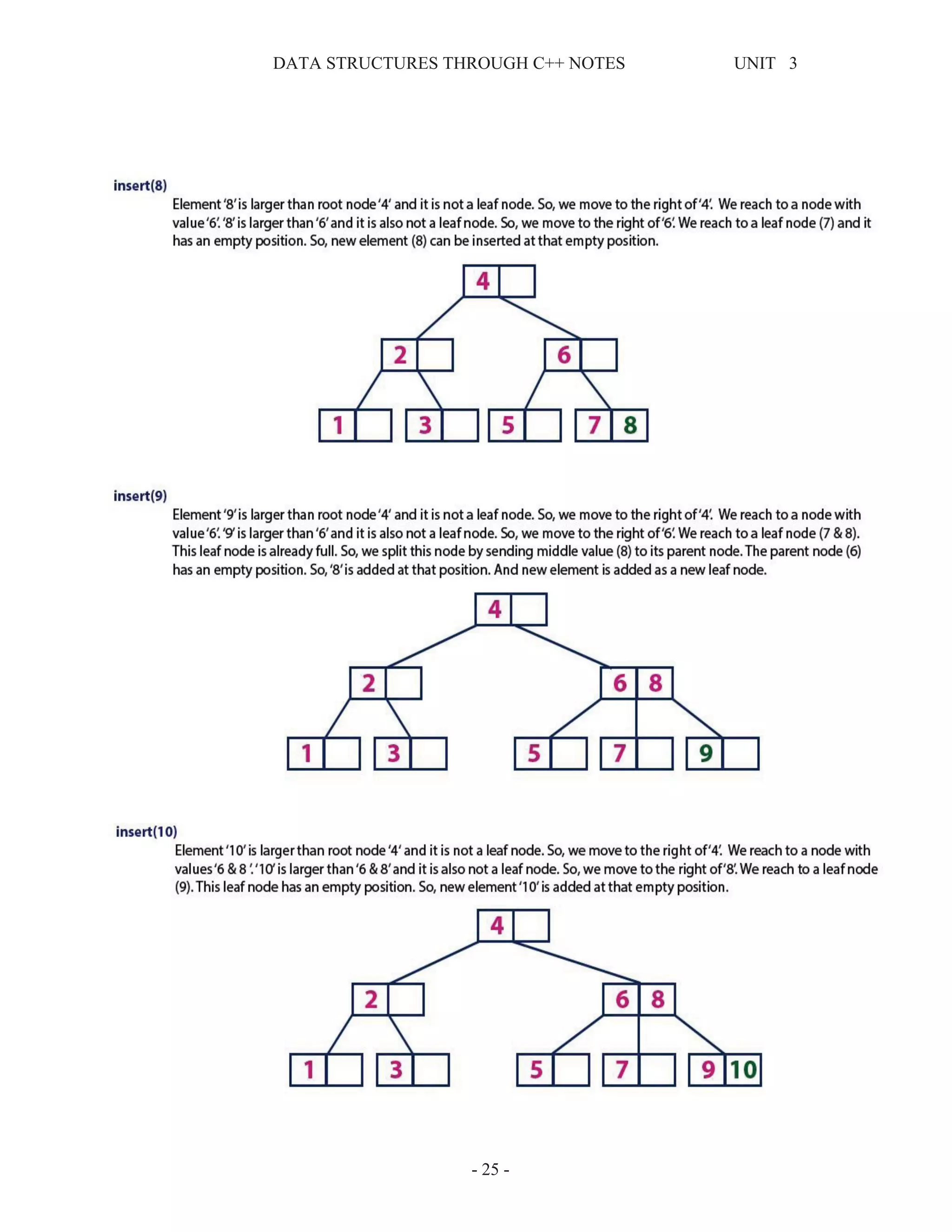
Example
Operations on a B-Tree
The following operations are performed on a B-Tree...
1. Search
2. Insertion
3. Deletion](https://image.slidesharecdn.com/dscunit3notes-190204060226/75/Dsc-unit-3-notes-21-2048.jpg)


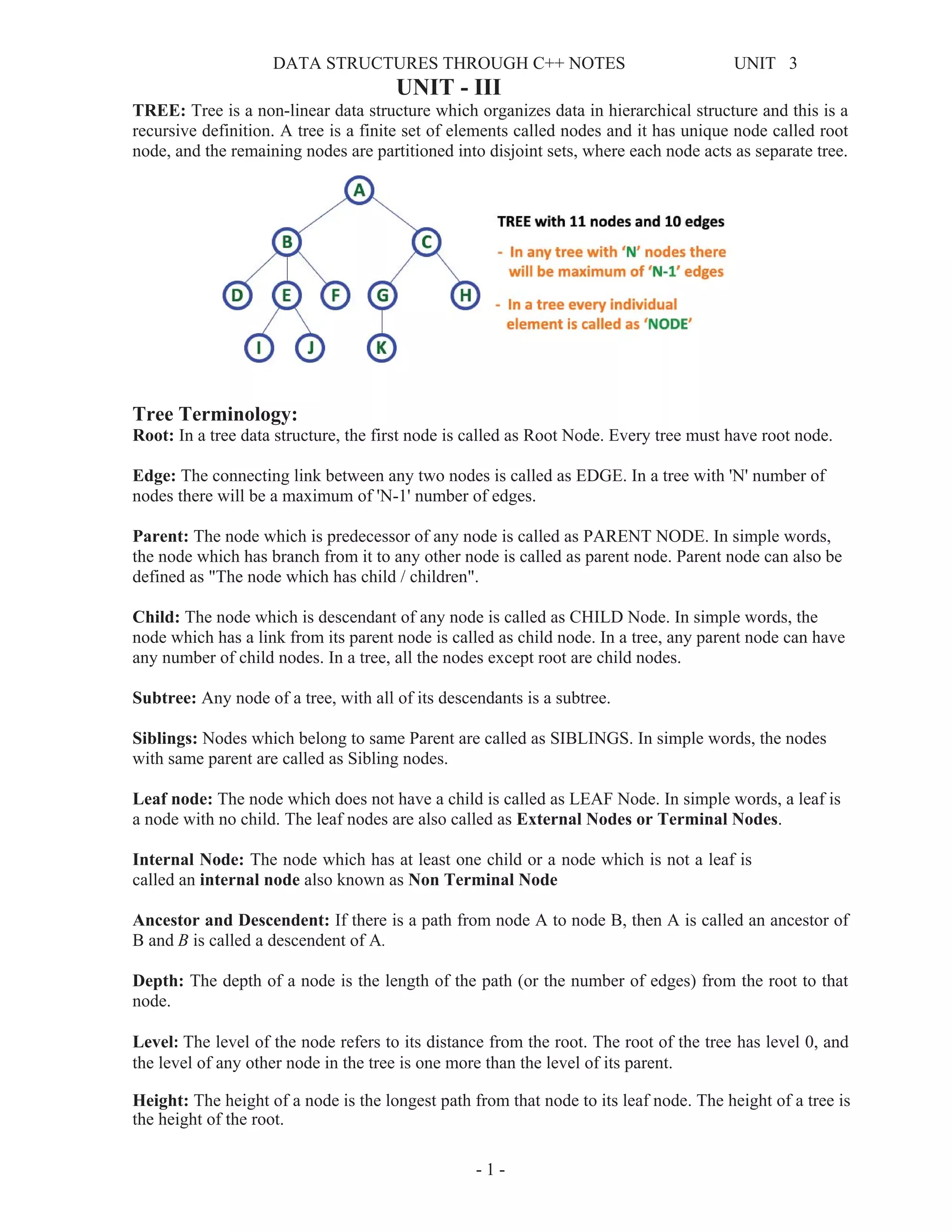
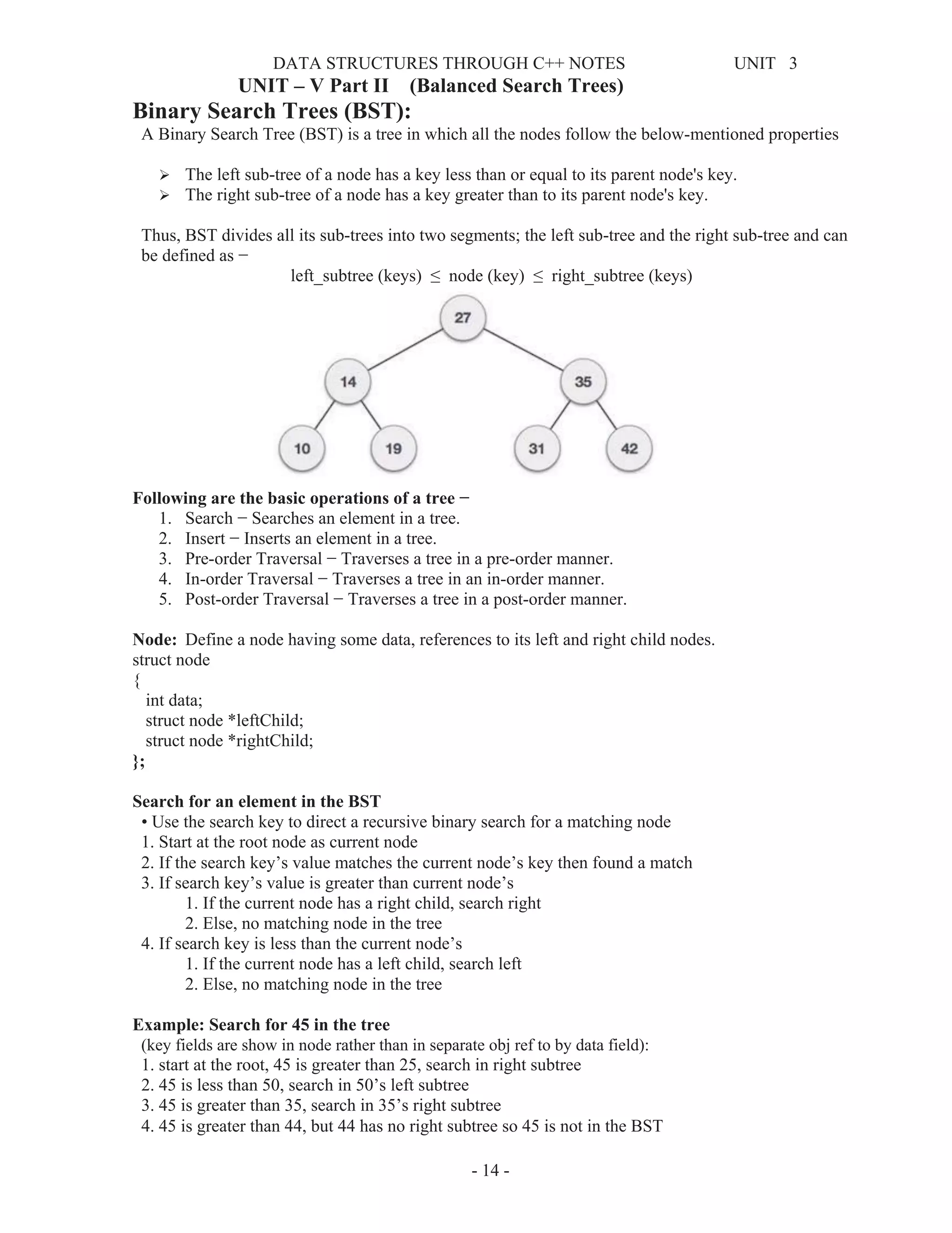
This document provides information about tree data structures. It defines key tree terminology like root, parent, child, leaf node, internal node, subtree, and siblings. It also describes different types of trees like binary trees, binary search trees, threaded binary trees, and heaps. Common tree traversal algorithms like preorder, inorder, and postorder are explained. Priority queues and their representations using heaps are also discussed.