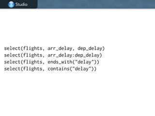
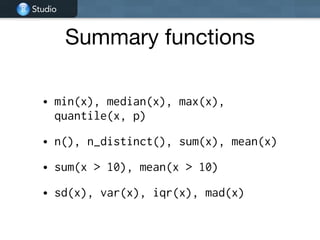
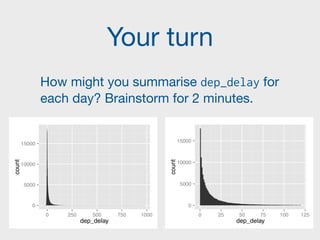
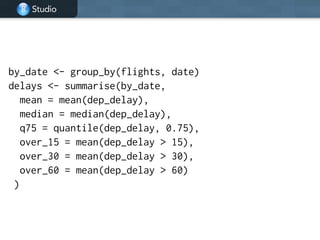
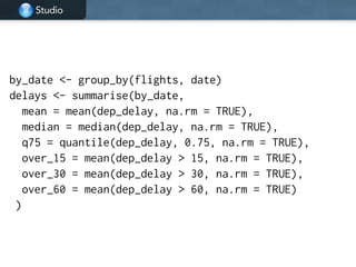
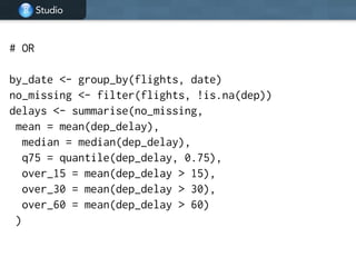
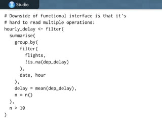
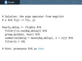
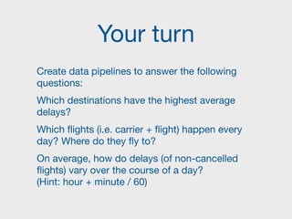
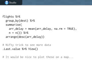
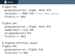
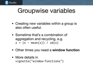
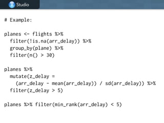
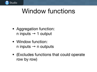
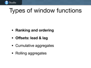
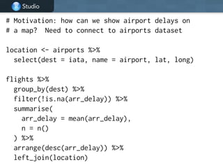
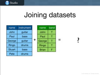
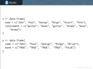
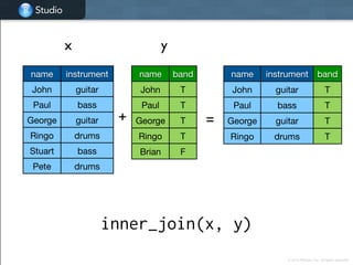
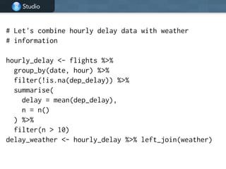
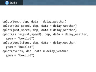
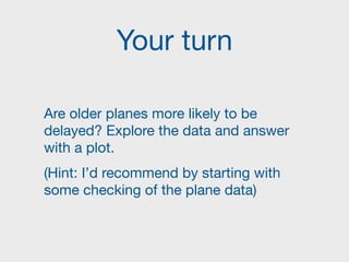
This document provides an overview of data manipulation techniques using the dplyr package in R. It begins with an introduction to core dplyr verbs like filter(), select(), arrange(), mutate(), and summarise() for manipulating single tables of data. It then demonstrates how to perform grouped operations using group_by() with summarise() and how to chain multiple operations together into data pipelines using the pipe operator %>%. Finally, it shows how to use grouped mutate() and filter() with window functions to create and filter rows based on group-level calculations. The document uses flights data to demonstrate these techniques throughout.


![Studio
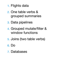
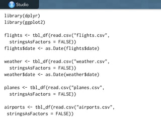
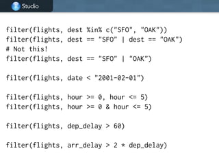
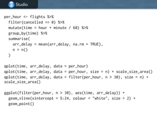
Flights data
• flights [227,496 x 14]. Every flight
departing Houston in 2011.
• weather [8,723 x 14]. Hourly weather
data.
• planes [2,853 x 9]. Plane metadata.
• airports [3,376 x 7]. Airport metadata.](https://image.slidesharecdn.com/dplyr-tutorial-220416011101/85/dplyr-tutorial-pdf-11-320.jpg)

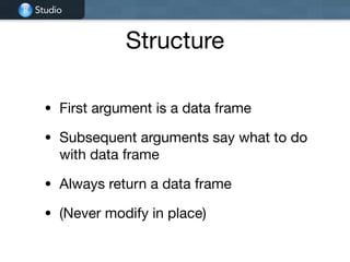

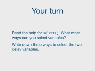


![Studio
# Derived from http://stackoverflow.com/a/23341485/16632
library(dplyr)
library(zoo)
df <- data.frame(
houseID = rep(1:10, each = 10),
year = 1995:2004,
price = ifelse(runif(10 * 10) > 0.50, NA, exp(rnorm(10 * 10)))
)
!
df %>%
group_by(houseID) %>%
do(na.locf(.))
!
df %>%
group_by(houseID) %>%
do(head(., 2))
!
df %>%
group_by(houseID) %>%
do(data.frame(year = .$year[1]))](https://image.slidesharecdn.com/dplyr-tutorial-220416011101/85/dplyr-tutorial-pdf-76-320.jpg)