Does the value-added tax shift to consumption prices?

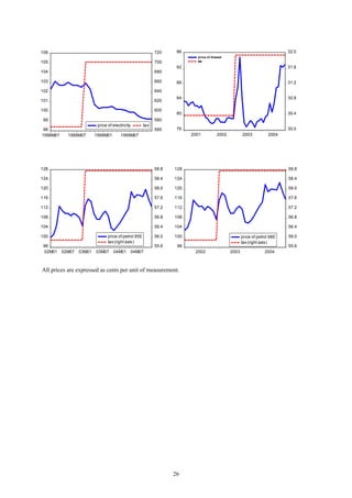
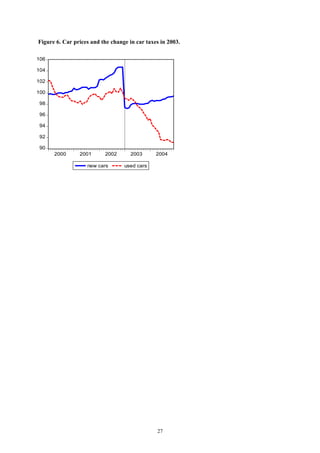
250
Does the
value-added
tax shift to
consumption
prices?
Matti Virén

PALKANSAAJIEN TUTKIMUSLAITOS •TYÖPAPEREITA
LABOUR INSTITUTE FOR ECONOMIC RESEARCH • DISCUSSION PAPERS
* Part of the study dealing with Finnish excise taxes has been carried out together with Emmi
Martikainen of the University of Vaasa. Tiina Teppala provided research assistance. The study
has benefited from useful comments from two anonymous referees, Heikki Kuitunen and Petri
Malinen, Jaakko Kiander, Pasi Holm and Hanna Karikallio, as well as from the members of a
Finnish research group on food taxation and participants of 2007 IIPF Congress in Warwick.
Financial support from the OP Bank Group Research Foundation and the Finnish Employee
Foundation is also gratefully acknowledged.
** Matti Viren, Department of Economics, and Public Choice Research Centre, 20014 University
of Turku, Finland, matvir@utu.fi, and Monetary Policy Department, Bank of Finland, Finland.
Helsinki 2009
250
Does the
value-added
tax shift to
consumption
prices?*
Matti Viren**

ISBN 978−952−209−067−6
ISSN 1795−1801

3
ABSTRACT
This paper deals with the question of how consumption taxes, especially the value-added tax, affect
consumption prices. The analyses are based on data from EU countries for the period 1970-2004. The
starting point is a conventional supply-demand analysis of the tax incidence problem. This problem is
solved using some simple price mark-up equations, Phillips curves and inflation forecast error
equations. All these equations are estimated from panel data from EU countries using different
estimators and variable specifications. In addition, an analysis is carried out with Finnish excise taxes
using commodity/outlet level micro data for the period 1997-2004. A general result of all analyses is
that about two thirds of a tax increase shifts to consumer prices. By contrast, there is less evidence on
shifts to producer prices
Keywords: Value-added tax, tax incidence, consumption taxes
JEL Code: H22
Forthcoming in AUCO Czech Economic review.
YHTEENVETO
Tutkimuksessa selvitetään, miten kulutusverot, erityisesti arvonlisävero, vaikuttavat kuluttajahintoi-
hin. Empiirinen osa perustuu EU-maita koskevaan aineistoon ajanjaksolta 1970-2004. Tutkimuksen
taustalla on tavanomainen kysyntä-tarjonta-analyysi verotuksen kohtaannosta. Kohtaanto-ongelmaa
selvitetään yksinkertaisten mark-up hinnoitteluyhtälöiden, Phillipsin käyrien ja inflaatio-odotusvirhei-
tä koskevien analyysien avulla. Kaikki yhtälöt estimoidaan EU15 -maiden paneeliaineistosta käyttäen
erilaisia estimaattoreita ja muuttujatäsmennyksiä. Tämän analyysin ohella selvitetään valmisteverojen
hintavaikutuksia Suomea koskevan hyödyke- ja toimipaikkakohtaisen mikroaineiston avulla. Aineisto
kattaa ajanjakson 1997-2004. Empiiristen analyysien tulos on se, että noin kaksi kolmannesta veroista
siirtyy kuluttajahintoihin. Sen sijaan tuottajahintoihin verotuksella ei näyttäisi olevan mainittavaa vai-
kutusta.

4
1. INTRODUCTION
This study deals with the incidence of consumption taxes. More precisely, the intention is to measure to
what extent taxes shift to consumer prices. A motivating factor for the analysis is an intention to lower
the VAT rate on food in Finland. Currently, the Finnish food VAT rate is one of the highest in the
European Union (17 per cent compared with an average rate of 6 per cent1
) , The implicit consumption
tax rate in consumption is the third highest in the EU27 (27.3 per cent compared with the average 19.9
per cent, cf. Eurostat (2008)). Partly because of this a study group was formed to analyse the
consequences of an eventual tax cut which is to take place in 2009.2
Changing the tax structure is
obviously a complicated matter that involves analysis of the demand patterns, income distribution,
market structure and so on. In this analysis we disregard all welfare aspects and concentrate solely on
the issue of tax incidence. For practical reasons we cannot analyze the whole issue of tax incidence but
we have to concentrate on question of how do changes in the VAT rate(s) shift to consumer prices?3
In terms of empirical analysis, the usual way to proceed would obviously be to scrutinise previous tax
changes. Unfortunately, very few cases exactly match the planned Finnish case, and only the recent
tax cuts in Sweden, Norway and Iceland are generally directly applicable to our purposes. Evidence
from the Swedish, Norwegian and Icelandic exercises is displayed in Figures 1 to 3. In Sweden, food
taxes were lowered in 1996 from 21 to 12 per cent (9 percentage points), which ought to have led to a
7.4 per cent fall in consumption prices if taxes had completely shifted to prices. The corresponding
immediate change in food prices was -6.6 per cent, which came quite close to this figure. In Norway,
the corresponding figures for the 2001 reduction were 24 and 12 per cent, with an implied price level
of -9.7 per cent. The comparable one-month change in prices turned out to be 8.9 per cent, which
again is practically identical to the implied value. Recent tax reform in Iceland (2001) included to a
lowering of the VAT from 14 (in some cases 24.5) to 7 per cent, which ought to have lowered the
consumption prices of food by (more than) 6.1 per cent. New data from Statistics Iceland reveals that
the immediate price effect is as high as -7.4 per cent. This, in turn, can be explained by the fact along
with the VAT tax cut, excise duties on imported and domestic food, excluding sugar and sweets, were
also abolished.
If instead the producer prices are scrutinized (using data from Statistics Sweden, Statistics Norway
and Statistics Iceland) one arrives at a striking result: the monthly change rates are either zero or
1
Six per cent corresponds to the population weighted average of VAT rates for food and beverages. The
unweighted average is 8 per cent. By comparison, the average US sales tax rate is 7.7 per cent. For a more
exhaustive comparison of tax structures, see Eurostat (2008) and Coenen et al. (2008)
2
A final report of group has already been published by Holm et al. (2007).
3
See e.g. Coenen et al. (2008) and Bye et al. (2003) for more analyses of tax reform effects.

5
negative. Thus, these data does not support the hypothesis that taxes would have shifted immediately
to (wholesale merchandisers’ and retailers’) costs.
Summing up, evidence from these three Nordic countries suggests that consumption taxes almost
entirely shift to prices (a general figure would be something like 90 per cent). It is often argued that
the price shift effect is not linear (tax cut effects differ from tax hike effects, or the effects depend on
the cyclical situation or the industry). Some support for this proposition is provided by Garbonnier
(2005). Results from the three Nordic countries do not, of course, tell anything about nonlinearity, but
they suggest that the tax cut effects do not completely disappear, as is sometimes argued in the media.
In the case of the Nordic countries, such a result would in fact very surprising. All these countries
have small open economies where competition is severe, partly because foreign competitors have
relatively easy access to them. Thus, we basically have a standard textbook example of commodity
markets where supply is infinitely elastic and demand – by the nature necessities – is almost inelastic
(see e.g. Swinton, J. and Thomas, C. (2001) and Jha (1998)). Under such circumstances one might
expect that the short-run price effect of the tax is indeed very large.4
Unfortunately, these three cases are the only that we are aware of and they do not allow sophisticated
econometric analysis. For this purpose we have to use other data sources. In fact, we use two
alternative data sets: data on the main VAT rates from the EU15 countries and, secondly, data on
Finnish excise taxes. The former data are annual and cover the period from 1970-2004, for which the
Finnish data are monthly and cover a large number of individual commodities and selling outlets (the
data are derived from the CPI database) for the early 2000s.
Naturally, we can also make use of previous empirical analyses of tax incidence. Useful summaries of
the results are provided for instance by Fullerton & Metcalf (2002), Besley & Rosen (1998) and
Morin (2005). These analyses mainly deal with specific commodity taxes. This largely reflects the
nonexistence of the VAT in the United States from where most studies come. As for the structure of
the VAT (and food, in particular), Morin (2005) is highly relevant. On the basis of these summaries it
seems fair to conclude that, as a rule, more than 50 per cent of taxes are shifted to consumer prices.
Here, the analysis of Besley and Rosen (1998) dealing with the effect of sales tax on prices in the
United States should perhaps be particularly emphasized. Besley and Rosen observed that in several
cases prices increase more than taxes. Thus, research results are broadly consistent with the recent
informal evidence from the Nordic countries. Of course, there are differences between research results
depending on factors such as the:
4
Because the price elasticity of demand for food is very low, food appears to be a product that should, according
to the Ramsey principle, be taxed more heavily than, for instance, services. This in turn may explain why there
has been reluctance in lowering the tax rate, even though distributional reasons might have favoured it.

6
– size of the market
– length of the inspection interval
– nature of commodities
– market structure.
– analytical framework
– sign of the tax change
From the point of view of the current analysis these facts are somewhat alarming, because the analysis
of aggregate VAT rates in the EU does not exactly correspond to an analysis of Finnish VAT rates for
food. Neither does the analysis of Finnish excise taxes exactly correspond to the policy proposal.
Finnish petrol, electricity and car markets surely have some special characteristics that have to be kept
in mind when interpreting the final results. In particular, the level of competition differs considerably
(compare e.g. electricity and petrol pricing).
Nonetheless, these are the best data sets currently available and we have work with them. This study
first analyses VAT rates and then Finnish excise taxes. Before these analyses we briefly present the
analytical framework and the estimating equations. Finally, some concluding remarks are provided at
the end of the paper.
2. ANALYTICAL FRAMEWORK
Let us focus on a single commodity c with demand and supply being equal to D and S.5 6
Moreover, let
us assume that the corresponding curves are of the form: D = (PC/P)
-d
and S = ((1-τ)PC/P)
s
, where d and
s are price elasticities, PC the price of commodity c and P the general price (or cost level). τ is the ad
valorem tax rate.7
Assuming now that D = S, we can derive the following equation for the price “mark-
up”:
5
Note that in the subsequent analysis we do not always examine individual commodities but sometimes
aggregates, or even total consumption. In this case we have to keep in mind that instead of individual prices we
have implicit price deflators. Moreover, taxes apply not only to consumption but also to part of investment and
public consumption, which aggravates the simultaneity problem. The implicit weights of the tax rate do not
exactly match the “weights” of the consumption price deflator.
6
Even though micro data are currently available on consumer prices (see e.g. Aucremanne, L & Dhyne, E.
(2004)), they do not cover sufficiently long time periods for follow-up studies of VAR changes.
7
Here we do not consider tax incidence in the case of different market structures, although the case of
monopolistic competition, for instance, could provide useful insights into the different results of tax shifting.
Take, for instance, the case in which tax shifting exceeds 100 per cent. It is hard to explain this kind of result by
anything other than a monopoly. (See the classic studies of Musgrave (1959) and Fullerton and Metcalf (2002)
for details.)

7
log(PC) = log(P) - αlog(1-τ), (1)
where the coefficient of the tax rate is simply the ratio of the price elasticities, that is: α = (s/(d+s)).8
Basically, we can simply estimate (1) to obtain α, assuming that we have data on P, τ and possible
control variables. Although the analysis is in principle straightforward, there are several problems. The
most obvious of these is related to the nature of the price margins, log(PC) - log(P). We have, in fact,
several price margins reflecting the fact that before consumption goods reach consumers they are
handled by primary producers, the industry and wholesale and retail merchandise companies. Thus, we
have the producer prices (PP) which reflect the prices of the industry and raw material prices which
reflect the prices of primary producers. The difference between consumer prices and producer prices
mainly reflects the costs of merchandise and retail companies and their profits, plus taxes, of course. In
principle, changes in consumption taxes could show up in all of these items (including consumer prices)
but the effects could even show up in the input prices of industry, including the raw material prices.
Irrespective of the way in which the prices margins are measured, it appears that they not stationary.
Thus, there is a trend-like change in almost all price margins starting from the beginning of the 1970s
and continuing until the end of the 1990s. Since then the margins seem to have levelled off although
Finland, Ireland and Spain represent notable exceptions to this rule (see Viren (2007) for details).
One explanation for the recent behaviour is the introduction of the Euro and the resulting change in
the competitive environment.9
Here we can do little to control for the change in the market structure and/or competitive
environment. The only thing we can do is to include a time trend as a proxy for the structural change
or to move to first log differences. Thus, we start with the following simple estimating equation:
log(PCit) = a0 + a1log(PPit) + (1-a1)log(PMit) + a2TAXit + a3t + uit (2)
where
8
If the tax rate applies to pre-tax prices the supply curve is of the form S = (PC/ (1+τ) P)
s
, and (1) is of the form
log(Pc) = log(P) + αlog(1+τ). A convenient way of interpreting the result would be an analysis of a monopoly-
monopsony firm which has the following profit expression: (1-τ)p(q(x))q(x)-w(x)x where τ denotes the
commodity tax, p denotes the selling price, q denotes the output, x the input and w the input price (input could
be e.g. an industrial product which is purchased by a retailer) . Then the FOC gives the following condition: p(1-
τ)(1+1/ε)q’ = w(1+1/θ) where ε is the price elasticity of demand and θ the price elasticity of input supply.
Clearly, the tax incidence depends on relative price elasticities ε, θ and the curvature of the production/cost
function, q’.
9
The long-run growth of the price margin may reflect similar tendencies in the functional distribution of income.
The results might, however, also reflect some measurement problems. If we compute the price margin in terms
of import prices we have to acknowledge that import prices typically only include commodities while consumer
prices have a large weight for services.

8
PC = consumer prices (private consumption deflator), PP = producer prices, or alternatively
wholesale prices in the empirical application, PM = import prices, TAX = log(1+τ) where τ = the
main VAT rate, or alternatively the weighted-average tax rate, WAR, that is used by the EU 10, t =
time trend and u = the residual
In equation (2), import prices can reasonably safely be considered exogenous (with the “pricing to
market” caveat) but with producer prices the assumption is not completely warranted. Producer prices
which basically represent the prices that the industry obtains from its product could also adjust if
wholesale or retail merchandise companies have enough market power. With producer prices we can
make an experiment by estimating a two equation model where also producer prices are allowed to
adjust to changes in consumption taxes. The model which is basically an extension of equation (2)
will be reported along with other estimation results in Table A4.
Above, (2) has been estimated in a level form by introducing the lagged dependent variable as an
additional regressor and together with log differences. In practice, only a0, a2 and a3 have been
estimated freely, because a1 has been calibrated to be 2/3.11
Thus, we actually try to explain the gross
price margin. Even so, we do also estimate an even simpler price change equation that takes the
following form:
∆log(PCit) = a0 + a1∆TAXit + uit. (2’)
In the case of aggregate consumer prices, we could obviously make use of the Phillips curve to verify
whether, in the context of this curve, we could identify the effect of a tax change, and whether the
effect comes close to that from equation (2). Thus, the subsequent analysis with the Phillips curve
(and with unexpected inflation) can be seen as some sort of robustness checks. Estimating a Phillips
curve requires the introduction of an output gap (or some other proxy for the real marginal costs) to
the equation estimating price level changes, which would otherwise in the currently standard New-
Keynesian hybrid form be of the following form:
∆log(PCit) = b1∆log(PCit-1) + b2∆log(PC
e
it+j) + b3∆TAXt + b4GAPit + eit, (3)
where
10
WAR refers to the weighted average (tax) rate, which is computed as a ratio between VAR receipts and the so-
called VAT base. In a sense, it represents a weighted average of different VAT rates and VAT exceptions.
11
By calibrating the values we have partly circumvented simultaneity problems that are related to unrestricted
estimation of (2). Estimation results were not overly sensitive for this calibration. Alternatively, we use IV
estimation (Table A4).

9
j = the time horizon of inflation expectations (forecasts), that is either 1, 1½ or 2, p+j = ∆log(PC
e
) =
inflation forecast and GAP = output gap12
When estimating this equation, we have used the OECD inflation forecasts for expected inflation.
This makes estimation somewhat easier (we do not need to impose the rational expectations’
orthogonality conditions), and thus instead of GMM we can use least squares or maximum likelihood.
In addition to (3), we also estimate a backward-looking Phillips curve where we have import prices as
an additional regressor to incorporate open-economy considerations.
Inflation forecasts can also be used in assessing how much unanticipated inflation is a consequence of
unanticipated changes in VAT rates. One cannot obviously say how well VAT rate changes are
known in advance in the OECD but, fortunately, we have forecasts that go two years ahead of the
forecasting period (e.g. forecasts that are made in autumn 2002 for the year 2004).
Forecast errors for different time horizons give us the following testing equation:
∆log(PCit) - ∆log(PC
e
it+j) = c1∆TAXit + c2GAPit + vit (4)
where again the time horizon of forecasts is ½, 1 and 2 years.
The parameters of interest in the estimation of (2), (3) and (4) are a2, b3 and c1. Although we might
not expect that they are exactly the same, we might nevertheless expect that they are of the same
magnitude and at least between 0 and 1.
The analysis now turns to Finnish excise taxes. As point out earlier, this analysis is carried out using
the micro level Consumer Price Index (CPI) data.
Here, the basic problem and thus also the analytical framework is the same as with aggregate
consumer prices. However, the frequency of the data is quite different (monthly) and the commodities
are genuinely different (commodity brand, weight and selling outlet). The estimation period is (with a
few minor exception) 2001M1-2004M12. Moreover, the number of observations is very large, going
up to thousands per commodity. The problem is that we are completely unable to construct a proper
price margin, let alone price change expectations. However, because we have monthly data we may
safely assume that producer prices (costs) do not change at the same time as taxes. Later on we see
that this might not be exactly true, but otherwise we may proceed with this assumption and thus
estimate the following very simple price equation (which is comparable to (2’)):
12
Output gaps are here constructed by means of the Hodrick-Presoctt filter with the usual weight parameter 100.

10
log(PCikt) = a0k + a1klog(taxkt) + uikt (5)
Notice that now index i indicates a single commodity (commodity brand or selling outlet; i.e. in the
case of unleaded 95-octane petrol the cross-section of observations corresponds to different petrol
stations; with beer we have both different shops and different brands/marks and bottle sizes) while k
denotes the commodity group. In some cases (electricity, petrol) we also include a proxy for the
producer prices to control for possible simultaneous cost changes.
The estimation period is so short that we may assume that other potential control variables constant. For
the same reason, no seasonals are included. In most cases, the data include only one change in taxes
which obviously diminishes the value of information. In is not uncustomary that the number of events is
this small. Take for instance the case of changes in legislation (cf. e.g. MacKinlay (1997)). Even so, we
have to consider the results as a whole rather than to focus on each individual coefficient estimate.
Although we have estimated equations (1) – (4) for single countries, here all reported analyses make
use of cross-country panel data. For practical reasons, we restrict the coefficients of the explanatory
variables to be the same so that we have a representative number for the tax shift parameter.
3. VAT RATE CHANGES IN EU COUNTRIES
The analyses have been carried out with annual panel data from 15 EU countries for the period 1970-
2004. In practice, the data include 393 data points when we use the main VAT rate as the tax
variable13
. We do also introduce the two reduced rates as explanatory variables but only the ordinary
reduced rate (typically for food) turns out to have explanatory power. When instead we use the WAR
data the number of data points goes down to 176 (see Figure 4 for the tax data). Annual data are
obviously not ideal for our purposes because in principle the tax rate change can in principle take
place at any time of year and the time path of prices can differ quite a lot between countries and years.
It seems, however, that almost all tax changes have taken place at the beginning of the year, which
makes the results somewhat comparable across countries.
The results are summarised in Table 1, while detailed results are reported in the Appendix (Tables
A1-A4). In Table 1, we report only the coefficient estimates of the tax variable and with
specifications (3) and (4), we just report the results with the longest time horizon for inflation
expectations (to minimize the possibility that advance announcement of tax changes would show up
in inflation forecasts). Anyway, a full set of results is reported in the appendixes.

11
In assessing and interpreting the results we have several problems. First we need to consider whether
the partial adjustment type of model is appropriate to capture the long-term effects of tax changes.
The nature of the data (i.e. annual frequency) already makes the distinction between short- and long-
run effects quite subtle. In the case the Phillips curve and forecast errors model, we cannot in a similar
way measure the long-run effects. Only if we consider the forecasts to be exogenous (with respect to
tax changes) we can technically compute the long-run values in the same way as in the case of
equation (2). Whether that can be done depends crucially on the economic rationalization of the
lagged term.
Interpretation of the Philips curve is rather complicated because in "free" estimation the sum of lag
and lead inflation terms exceeds unity. However, the problem does not appear to be particularly
severe and similar problems have been encountered in almost all empirical applications of Phillips
curves.14
One might argue that the Phillips curve is not best way to identify tax effects, because if tax changes
are known in advance they obviously show in expected inflation. Only if we use a sufficiently long
time horizon for expected (forecasted) inflation could we perhaps circumvent this problem. Results
with an unanticipated inflation model seem indeed to corroborate this projection. Thus, the longer is
the time horizon in making inflation forecasts, the higher is the tax rate coefficient. In the case of a
two-year horizon, the coefficient is of the magnitude of 0.75, which makes sense according to other
empirical analyses and also informal evidence from the Nordic countries.
The system estimation results (reported in Table A4) give some idea of the nature of tax incidence in
general. It seems that taxes have a very strong impact on consumer prices (the long run effect is even
slightly above one) while the effect on producer prices is quite weak (and statistically) insignificant
although it is of correct sign. Thus, the casual observations which were mention in section 1 for the
Nordic countries’ experiences with a lower VAT for food seem to be consistent with more general
empirical evidence. In other words, the VAT seems to shift mainly to consumer prices, not producer
(and presumably not to raw material) prices.
The empirical results can perhaps be summarized by saying that in general the coefficients of the tax
variable fall within the range of 0.4 to 0.8. The coefficients are practically always positive and equally
regularly below 1. Moreover, one may safely reject the hypothesis that the coefficient is just zero.
Thus, taxes shift to prices: if not completely, more than half of the effect shows in prices.
____________________
13
The EU allows for two reduced rates: a reduced rate and a special reduced rate. The rates should in principle
exceed 5 per cent but some countries have received permission to apply even lower (zero) rate.
14
Compare e.g. to the results of Paloviita & Viren (2005) and Tillman (2005).

12
Here, it should be kept in mind that the results are not directly applicable to any specific tax rate
change in any specific country. Changes in the main VAT rates apply to all kinds of goods with a
wide variety of demand and supply elasticities. Thus, for instance, they include services where
demand elasticities might well be larger than supply elasticities. This, in turn, would show in lower
values of the tax-shifting parameter which should be kept in mind when considering policy proposals
which intend to improve employment, for instance.
Table 1. Summary of results from EU data.
Specification Estimator Tax rate Tax rate coefficient
Price margin equation (2) â2
Level form; short run GLS,FE VAT1 .200
Level form: long run GLS,FE VAT1 .753
Level form; short run GLS,FE VAT1&2 .163*
Level form; long run GLS,FE VAT1&2 .898*
Level form; short run GLS,FE VAT1 .099
Level form; long run GLS,FE VAT1 .414
Level form; short run GLS,FE VAT1&2 .118*
Level form; long run GLS,FE VAT1&2 .494*
Difference form GLS VAT1 .942
Difference form GLS, FE VAT1 .428
Difference form GLS VAT1 1.017
Difference form GLS, FE VAT1 .579
Level form, no lags 0LS VAT1 .442
Level form; no lags IV$
VAT1 .817
Level form, lags, long-run IV$
VAT1 .875
Arellano-Bond GMM, long run GMM VAT1 .717
Phillips curve equation (3) ^ b3
unrestricted estimates OLS VAT1 .443
unrestricted estimates GLS VAT1 .360
unrestricted estimates SUR VAT1 .449
b1+b2 = 1 OLS VAT1 .537
b1+b2 = 1 GLS VAT1 .401
b1+b2 = 1 SUR VAT1 .409
Unanticipated inflation equation (4) ĉ3
OLS VAT1 .746
GLS VAT1 .433
SUR VAT1 .721
See the appendixes for details. All level from equations include a time trend, while the first difference models
include only a constant term (fixed effects, FE) or nothing. With inflation expectations, the forecast horizon for
∆log(PCe
it+j) is in all cases S3 which means that the forecasts are made in December (year t) for the year t+2.
* denotes the sum of the coefficients of the main VAT rate and the reduced rate. $) In the IV estimation, the
dependent variable is log(PC), not the price margin. The data represent the EU15 countries.

13
Between-country differences should also be considered. For small open economies, it is quite
clear that the supply of goods is almost perfectly (price)elastic, while in large countries this
assumption is not equally warranted. Thus, the tax incidence parameters would also differ
accordingly, being probably larger in small countries.15
But again we have a caveat: retail trade
appears more concentrated in small countries, which might also imply a lower level of
competition (DG Competition (1999)). It is not, however, clear whether concentration indexes
(measured as market shares of companies) are equivalent to indices of competition. This doubt
arises when scrutinizing the development of concentration indices: they tend to generally steadily
increase in the EU15, but this does not seem to show in price margins or in other indicators of
competition.
4. FINNISH EXCISE TAXES
The structure of the Finnish commodity tax system the following: The main tax is the Value-Added-
Tax with the general rate 22 %. The reduced rate for food is 17 % and the special reduced rate for
books, drugs and transportation is 8 %. Subscriptions for newspapers are tax except. In addition to the
VAT, there are excise taxes for the following commodity groups: tobacco, alcohol, electricity,
gasoline and cars. The corresponding tax rates are also relatively high. The exact rates cannot be
quoted here because most of these taxes are combined ad valorem and unit taxes (see Martikainen and
Viren (2006) for more details).
This analysis deals with the following CPI commodity groups: alcohol, cars (new and used), petrol
(95 and 98 octane) diesel, beer, long drink, cider and electricity.16
The empirical results for estimating
equation (5) are presented in Table 2. Moreover, the tax changes are illustrated in Figure 5. The prices
changes of old and new cars are illustrated in Figure 6.
On the basis of the figures and estimation results one may readily conclude that (a) the magnitude by
which taxes shift to prices varies considerably between products/branches and (b) the short-run tax
parameter falls short of one, being roughly of the magnitude of two thirds.
15
A relatively well-documented case is that of oil prices. The supply of oil is essentially perfectly elastic with
respect to small countries or market areas, while for the world supply elasticity is much lower. Thus, it makes a
considerable difference whether individual countries or all countries impose taxes on oil consumption. See
Chouinard and Perloff (2004) for US evidence.
16
Here we have omitted tobacco which is a bit complicated because of different tax rates for different tax
products. Moreover, pricing is highly regulated which produces an almost trivial result (Viren 2007). Thus, in
monthly data, only the tax changes show up.

14
These results are not, of course, in any way surprising given the differences in market structure and
competition between branches. Moreover, we have to keep in mind that with items such as electricity,
long-term contracts hide the price effects for several months. By contrast, in the case of alcohol, all
retails sales take place in the Finnish state monopoly, the Alko Company, which in practice means
that taxes shift almost exactly to prices.17
The change in car taxation in 2003 represents an interesting episode in the incidence of consumption
taxes. It appears that car taxes have only marginally shifted to prices. This is especially true with used
cars (see Figure 6). Closer scrutiny of car prices reveals some interesting insights into car pricing. In
the past, when Finnish car taxes were extremely high (more than 100 per cent of the pre-tax price),
car producers and import firms tried to keep the import prices as low as possible. Thus, the pre-tax car
prices were among the lowest in Europe and much lower than, for instance, in Germany. Along with
the lowering of car taxation, import prices started to increase (cf. Viren 2007). In other words, earlier
car producers, importers and sellers paid part of the tax but lower taxes also allowed them to obtain a
better price. Scrutinizing the profitability of cars to importers/sellers suggests that, after all, profits
slightly increased in 2003 despite marked decreases in retail prices.18
The government also benefited
from the tax cut, as receipts from car taxes increased by 18 per cent in 2003 (for more details, see
Martikainen and Viren (2006)).
17
The state monopoly applies only to retail sales to consumers; pricing of hotel/restaurant alcohol is not
considered in this study.
18
If taxes are set on import prices, producers can have a strong incentive to set up a sister company to import
cars. The sister company can then have higher profit margins, which are nevertheless taxed at a lower rate then
imported cars. This pricing strategy explains at least part of the change in pre-tax car price differentials over
time. For the data, see European Commission (2005).

15
Table 2. Results with Finnish CPI data.
TAX Brent/TH R2/SEE N pre-tax rate Ad valorem
alcohol 1.022
(1290)
1.000
0.000
12 200 .999
cars (new) .700
(20.11)
0.990
0.040
720 7500 .873
cars (used) .183
(8.03)
0.856
0.003
12 7500 .224
petrol 95E .662
(10.23)
0.460
0.036
1224 34 .402
petrol 95E .313
(4.82)
.161
(13.77)
0.538
0.033
1224 34 .190
petrol 98E .738
(12.76)
0.562
0.035
1224 36 .459
petrol 98E .344
(5.17)
.154
(13.20)
0.540
0.033
1224 36 .253
diesel 2.422
(17.41)
0.360
0.060
1200 32 1.988
diesel .420
(3.64)
.499
(33.16)
0.680
0.042
1200 32 .345
beer .829
(48.12)
0.991
0.023
467 45 .748
long drink .685
(21.24)
0.696
0.048
874 90 .824
cider .691
(42.16)
0.856
0.029
1063 83 .661
electricity 1.799
(12.56)
0.940
0.0002
12 5850 2.154
electricity .894
(4.18)
.615
(7.36)
0.915
0.003
12 5850 1.074
The pre-tax price is expressed in cents, with cars in euros. Koskenkorva spirits is used as the
benchmark product for alcohol. The average price of imported cars is slightly above 9000 euros.
“Brent” refers to the Brent oil price and TH to the producer price, which has been used in constructing
the price margin. N denotes the number of data points and numbers inside parentheses the White-
corrected t-ratios. The tax rate is expressed in the log(1+(tax/pre-tax price)) form. The corresponding
ad valorem tax rate effects are presented in the last column of the table. Computing the tax rates has
been somewhat cumbersome because no time series of the tax rates are available and in legislation
taxes are expressed in either Finnish markkas or in Euros/cents (sometimes in percentage terms). See
Martikainen and Viren (2006) for more details of the computation of these tax rates.
The Finnish car tax reform clearly illustrates the errors that are induced when using tax receipts (in
relation to some scale variable such as the GDP) as an indicator of the severity of taxation. If taxes are
simply too high, preventing sales, one may misleadingly interpret low level of tax receipts an
indication of the lightness of taxation, even if the opposite is true.

16
Considering all taxes, we may we conclude that, in accordance with the results for consumption prices
in the EU, excise taxes shift to prices in a way that justifies using the range from 60% to 100% as the
confidence interval and 80% as a representative estimate.
5. CONCLUDING REMARKS
Most of consumption taxes seem to shift to consumer prices. This finding is corroborated by all
analyses that we have made19
. Although our analyses all pointed in the same direction and indicated
that tax shifting is of the same magnitude as in most previous analyses, we must acknowledge several
caveats that complicate more affirmative conclusions.
First of all, in the European data we cannot control such important elements as excise taxes, various
tax deductions and exceptions. Neither do we have data for market structures or competitiveness
(such as Herfindahl indices). The frequency of the data also prevents proper analysis of immediate,
medium-term and long-term effects. Nevertheless, we can argue that evidence from tax incidence is
sufficiently compelling to nullify arguments that taxes do not show up in consumer prices or that the
tax shifting effect is negligible. In considering estimates of the tax rate coefficient from the point of
view of Finnish food prices, one has to keep in mind that Finland is a small open country and in this
respect deviates somewhat from, say, Germany and France. The level of competition is otherwise
difficult to compare, but casual evidence does not seem to suggest that the Finnish markets work less
perfectly then elsewhere in Europe.
Whether this is enough to justify changes in certain specific (here food) tax rates is unclear, because
the decision ultimately depends on estimates of the welfare effects. To some extent these effects have
been evaluated, but even then more analysis and public debate are still needed.
REFERENCES
Bye, B., Strom, B. and Åvitsland, T. (2003) Welfare Effects of VAT Reforms: A General Equilibrium
Analysis. Statistics Norway Discussion Paper 343.
Aucremanne, L & Dhyne, E. (2004) How Frequently Do Prices Chance? Evidence Based on the
Micro Data underlying the Belgian CPI. ECB Working Paper 331.
19
An unweighted average of all (long-run) estimates tabulated in this paper is 0.64. The corresponding median is
0.60.

17
Besley, T and Rosen, H. (1998) Sales Taxes and Prices: An Empirical Analysis. NBER Working
Paper No. 6667.
Carbonnier, C. (2005) Is Tax Shifting Asymmetric? Paris-Jourdan Sciences Economiques Working
paper 34/2005.
Chouinarnd, H. and Perloff, J. (2004) Incidence of Federal and State Gasoline Taxes. Economics
Letters 83, 55–60.
Coenen, G., McAdam, P. and Straub, R. (2008) Tax Reform and Labour Market Performance in the
Euro Area: A Simulation based analysis using New Area-Wide Model, Journal of Economic
Dynamics and Control 32(8), 2543-2583.
DG Competition (1999) Buyer Power and Its Impact on Competition in the Food Retail Distribution
Sector in the European Union. A report prepared by Dobson Consulting.
http://ec.europa.eu/comm/competition/publications/studies/bpifrs/.
European Commission (2005) Competition : convergence of car prices in the euro zone.
http://europa.eu.int/comm/competition/car_sector/price_diffs/.
Eurostat (2008) Taxation Trends in the European Union.
Fullerton, D. and Metcalf, G. (2002) Tax Incidence. In Handbook of Public Economics 4, Auerbach,
A. and Feldstein, M. (eds.), Elsevier Science, Amsterdam, 1787-1872.
Holm. P., Kiander, J., Rauhanen, T. and Viren, M. (2007) The Effects of Lowering the VAT Rate for
Food (in Finnish, the Finnish title “Elintarvikkeiden arvonlisäkannan alentamisen vaikutukset”). PTT
Reports 200.
Jha, R. (1998) Modern Public Economics. Rutledge, London.
MacKinlay, J. (1997) Event Studies ain Economics and Finance. Journal of Economic Literature 35,
13-39.
Martikainen, E. and Viren, M. (2006) The Shift of Excise Taxes to Consumption Prices in Finland in
1997-2004 (in Finnish, the Finnish title “Valmisteverojen välittyminen kuluttajahintoihin Suomessa
1997-2004”). VATT Discussion Paper 397.
Morin, M. (2005) Samhällekonomiska effecter vid genomförandet av ed budgetneutral förändring av
momsstrukturen – motoder och utgångspunkter. In SOU2005:57, Bilaga 5.
Musgrave, R. (1959) The Theory of Public Finance. McGraw-Hill, New York.
Paloviita, M. and Viren, M. (2005) The Role of Expectations in the Inflation Process in the
Euro Area. Bank of Finland Discussion Papers 5/2005.
Swinton, J. and Thomas, C. (2001) Using Empirical Point Elasticities to Teach Tax Incidence. Journal
of Economic Education , 356-368.

18
Tillmann, P. (2005) The New Keynesian Phillips Curve in Europe: Does It Fit or Does It Fail?
Deutsche Bundesbank Discussion Paper 4/2005, forthcoming in Empirical Economics.
Viren, M. (2007) Analyzing the incidence of consumption taxes. Pellervo Research Institute Working
Paper 97.

19
Table A1. Estimation results from the price margin equation (2).
Equation TAX1 TAX2 Time trend Lagged dependent
variable
R2
/SEE DW
Level, PP, FE .442
(2.18)
.013
(26.91)
0.996
0.050
0.42
Level, PP, FE .200
(1.38)
.003
(5.42)
.735
(20.82)
0.999
0.028
1.33
Level, PP, FE .163
(1.10)
.075
(1.44)
.003
(5.32)
.735
(20.62)
0.999
0.028
1.34
Level, WP, FE .099
(0.92)
.003
(5.29)
.761
(20.92)
0.996
0.025
1.38
Level, WP, FE .074
(0.67)
.044
(0.76)
.003
(5.14)
.761
(20.84)
0.971
0.025
1.39
Dif, FE .753
(2.79)
0.132
0.041
0.31
Dif, FE .110
(1.02)
.871
(35.49)
0.816
0.020
1.66
Dif, PP .942
(3.69)
..
0.032
1.22
Dif, PP, FE .428
(1.88)
0.056
0.030
1.46
Dif, WP 1.017
(4.84)
..
0.029
1.19
Dif, WP, FE .579
(3.26)
0.049
0.026
1.50
The price (m) marginal is derived as: m = log(PC) – 0.67*log(PB) – 0.33 log(PM). TAX = log(1+tax). Level refers
to the level from the equation and Dif to the first difference specification. In equations 4 and 5 (see the
corresponding lines), log differences of the consumer prices (not price margins) are first used. All estimates are
cross-section GLS estimates. TAX1 denotes the main VAR rate and TAX2 the reduced rate. PP denotes
producer prices and WP wholesale prices that used as the right-hand-side variable.

20
Table A2. Estimation of the Phillips curve (3).
Equation,
time horizon
p+i
e
p-1 ∆TAX GAP pm R2
/SEE DW
OLS, S3 .545
(5.36)
.531
(8.11)
.443
(2.77)
.098
(2.88)
0.911
0.899
2.35
GLS, S3 .534
(12.17)
.521
(16.12)
.360
(3.66)
.092
(4.63)
0.909
0.933
2.13
SUR, S3 .551
(36.21)
.522
(66.40)
.449
(18.93)
.097
(11.78)
0.911
0.942
1.96
OLS, S3 .339 .661
(15.09)
.537
(2.86)
.125
(3.91)
0.915
0.906
2.03
GLS, S3 .412 .588
(19.02)
.401
(3.43)
.120
(6.20)
0.909
0.886
2.07
SUR, S3 .423 .577
(16.74)
.409
(4.90)
.133
(8.15)
0.967
1.425
2.03
OLS, K2 .596
(7.48)
.431
(6.79)
.252
(1.55)
.103
(3.43)
0.912
0.953
2.21
GLS, K2 .613
(13.04)
.411
(11.69)
.304
(3.84)
.102
(4.55)
0.911
0.950
0.95
SUR, K2 .582
(19.32)
.435
(19.80)
.258
(5.69)
.117
(8.23)
0.911
0.959
2.17
OLS, S2 .760
(16.35)
.312
(8.13)
.198
(2.76)
.050
(1.56)
0.932
1.175
2.17
GLS, S2 .730
(18.67)
.326
(10.85)
.202
(4.64)
0.33
(1.38)
0.931
1.167
2.14
SUR, S2 .715
(25.17)
.342
(16.20)
.189
(5.57)
.056
(3.16)
0.932
0.943
2.15
OLS .775
(38.70)
.169
(1.44)
.242
(7.39)
.200
(12.53)
0.895
1.471
2.09
GLS .791
(54.04)
.086
(1.50)
.223
(9.32
.165
(12.89)
0.892
0.943
2.13
SUR .799
(62.94)
.085
(1.11)
.269
(9.44)
.178
(12.92)
0.894
1.456
2.03
OLS denotes the least squares estimator, GLS the cross-section generalized least squares estimator and SUR the
comparable, seemingly unrelated regression estimator. ∆TAX = ∆log(1+tax), p+i = ∆log(PCe
t+i ), p-1 = ∆log(PCt-i)
and pm = ∆log(PMt ) where PM denotes import prices. K2, S2 and S3 denote OECD’s inflation forecasts. S2
denotes the December forecast for the next year and S3 the corresponding forecast for the following year.
Analogously, K2 denotes the June forecast for the next year.

21
Table A3. Estimation results from the forecast error model (4).
Estimator,
time horizon
∆TAX GAP R2
/SEE DW
OLS, S3 .746
(2.22)
.239
(4.59)
0.157
1.321
1.32
GLS, S3 .433
(2.14)
.224
(7.72)
0.146
1.304
1.41
SUR, S3 .721
(17.17)
.215
(12.89)
0.156
0.936
1.92
OLS, K2 .413
(2.56)
.153
(3.94)
0.086
1.264
1.57
GLS. K2 .441
(3.37)
.143
(4.84)
0.086
1.263
1.77
SUR K2 .408
(6.31)
.122
(7.30)
0.083
0.955
1.80
OLS, S2 .082
(0.51)
.209
(4.52)
0.039
1.768
1.51
GLS, S2 044
(0.38)
.169
(5.13)
0.036
1.554
1.55
SUR, S2 -.001
(0.01)
.150
(6.38)
0.031
0.952
1.87
OLS, S3, WAR .628
(1.23)
.234
(6.05)
0.157
1.175
1.59
GLS, S3, WAR .442
(1.93)
.205
(8.17)
0.152
1.168
1.39
OLS, K2, WAR .373
(1.09)
.164
(5.54)
0.171
0.816
1.52
GLS, K2, WAR .389
(2.02)
.151
(6.52)
0.170
0.815
1.65
OLS, S2, WAR .317
(1.23)
.087
(3.28)
0.069
0.761
1.56
GLS, S2, WAR .259
(1.47)
.065
(2.93)
0.065
0.758
1.69
∆TAX = ∆log(1+tax) where both the main VAT rate (VAT1) and the weighted average rate (WAR) are used.

22
Table A4. IV, GMM and system estimates.
IV estimates of the level form equation
log(PC) = 1.014log(PP) + .817log(1+tax)
(48.9211) (4.12)
R2
= 0.991, SEE = 0.032, DW = 0.46
log(PC) = .082log(PP) + .819log(PC-1) + .125log(1+tax)
(2.92) (34.28) (1.66)
R2
= 0.998, SEE = 0.014, DW = 0.75
The set of instruments include gap, log(pp-1) and log(wpiUS)
Arellano-Bond GMM estimates for the price margin (m) equation
log(m) = .601log(m-1)+ .286log(1+tax) + .005t
(98.98) (10.32) (35.01)
R2
= .885, SEE = 0.028, J(11) = 9.30
The set of instruments include, in addition to lagged variables, m-2, gap, log(PMUS) and
log(WP). Time series have been transformed by using orthogonal deviations. J denotes the J
test for overidentifying restrictions.
System estimates with the two-equation model
∆log(PC) = .004 + .135∆log(PM) + .700∆log(PC-1) + .819∆log(PP-1) + .037∆log(1+tax)
(4.20) (9.19) (24.98) (1.71) (3.76)
R2
= 0.886, SEE = 0.011, DW = 1.67
∆log(PP) = .003 + .533∆log(PM) + .158∆log(PC-1) +.247∆log(PP-1) - .031∆log(1+tax)
(1.51) (18.78) (2.76) (5.55) (0.13)
R2
= 0.723, SEE = 0.021, DW = 1.89

23
Figure 1. Response of Swedish consumption prices to a tax cut in 1995/1996.
Change in food prices in Sweden in response
to a 9 % tax cut
-14 -12 -10 -8 -6 -4 -2 0 2
CPI total
food & beverages
bread
meat
fish
milk
oils
fruit
vegetables
sweets
other food
Figure 2. Response of Norwegian consumption prices to a tax cut in 2001.
Change in Food prices in Norway in response
to a 12 % tax cut
-16 -14 -12 -10 -8 -6 -4 -2 0
CPI
food & beverages
beverages
coffee
other food
sweets
vegetables
fruit
oil, grease
milk
fish
meat
bread

24
Figure 3. Response of Icelandic consumption prices to a tax cut in 2007.
Change in food prices in Iceland in respose
to a 7 % cut in taxes
-20 -15 -10 -5 0
CPI
food & beverages
food
bread
meat
fish
milk
oils and fats
fruit
vegetables
sugar
other
beverages
Figure 4. Median of VAT rates in the EU15.
10
12
14
16
18
20
22
1970 1975 1980 1985 1990 1995 2000
main VAT rate, % WAR, %

25
400
600
800
1000
1200
1400
1600
2001 2002 2003 2004
price of alcohol tax
20
40
60
80
100
120
140
2001 2002 2003 2004
price of beer tax
40
80
120
160
200
240
280
02M01 02M07 03M01 03M07 04M01 04M07
price of long drink tax
50
100
150
200
250
02M01 02M07 03M01 03M07 04M01 04M07
price of cider tax
Figure 5. Effect of excise taxes on consumer prices.

26
All prices are expressed as cents per unit of measurement.
98
99
100
101
102
103
104
105
106
560
580
600
620
640
660
680
700
720
1998M01 1998M07 1999M01 1999M07
price of electricity tax
76
80
84
88
92
96
30.0
30.4
30.8
31.2
31.6
32.0
2001 2002 2003 2004
price of disesel
tax
96
100
104
108
112
116
120
124
128
55.6
56.0
56.4
56.8
57.2
57.6
58.0
58.4
58.8
02M01 02M07 03M01 03M07 04M01 04M07
price of petrol 95E
tax(right axis)
96
100
104
108
112
116
120
124
128
55.6
56.0
56.4
56.8
57.2
57.6
58.0
58.4
58.8
2002 2003 2004
price of petrol 98E
tax(right axis)

27
Figure 6. Car prices and the change in car taxes in 2003.
90
92
94
96
98
100
102
104
106
2000 2001 2002 2003 2004
new cars used cars

Does the value-added tax shift to consumption prices?

More Related Content

What's hot

Viewers also liked

Similar to Does the value-added tax shift to consumption prices?

More from Palkansaajien tutkimuslaitos

Recently uploaded

Does the value-added tax shift to consumption prices?