This document discusses a phenomenon called "distinction bias" where people overpredict the difference in happiness between alternatives when making predictions or choices in a "joint evaluation" mode, compared to their actual experiences in a "single evaluation" mode. It proposes that people's evaluations of attributes can vary systematically between joint and single evaluation modes. When predicting or choosing, people compare options directly, leading to steep evaluation curves, but when experiencing an option directly, evaluations are flatter. This can lead to overpredicting differences between options during joint evaluation. The paper explores this distinction bias effect and when it does and does not occur.

1. Distinction Bias: Misprediction and Mischoice Due to Joint Evaluation
Christopher K. Hsee and Jiao Zhang
University of Chicago
This research identifies a new source of failure to make accurate affective predictions or to make
experientially optimal choices. When people make predictions or choices, they are often in the joint
evaluation (JE) mode; when people actually experience an event, they are often in the single evaluation
(SE) mode. The “utility function” of an attribute can vary systematically between SE and JE. When
people in JE make predictions or choices for events to be experienced in SE, they often resort to their
JE preferences rather than their SE preferences and overpredict the difference that different values of an
attribute (e.g., different salaries) will make to their happiness in SE. This overprediction is referred to as
the distinction bias. The present research also specifies when the distinction bias occurs and when it does
not. This research contributes to literatures on experienced utility, affective forecasting, and happiness.
Suppose that a person is faced with two job offers. She finds one
job interesting and the other tedious. However, the interesting job
will pay her only $60,000 a year, and the tedious job will pay her
$70,000 a year. The person wants to choose the job that will give
her the greatest overall happiness. To make that choice, she tries to
predict the difference in happiness between earning $60,000 a year
and earning $70,000 a year and also predict the difference in
happiness between doing the interesting job and doing the tedious
job. Is she able to make these predictions accurately? Is she able to
choose the job that will indeed bring her the greater overall
happiness?
Consider another example. A person currently lives in a 3,000-
square-foot (ft2
) house that is within walking distance to work. He
has the option to move to a 4,000-ft2
house for the same price as
his current house, but if he moves there, it will take him an hour
to drive to work every day. To decide whether to move, he tries to
forecast the difference in happiness between living in the 3,000-ft2
house and living in the 4,000-ft2
house and also to forecast the
difference in happiness between being able to walk to work and
having to drive an hour to work. Is he able to make these predic-
tions accurately? Is he able to make a decision that will give him
the greater overall happiness?
More generally, if people are presented with two alternative
values of an attribute, are they able to accurately predict the
difference these values will make to their happiness? If people are
faced with two options involving a trade-off along two attributes,
are they able to choose the option that will bring them the greater
overall happiness?
These are fundamental questions about affective forecasting and
about choice, and they are among the most enduring and signifi-
cant questions in psychology. These questions are relevant in a
wide range of domains, for example, when people decide which
career to pursue, when voters decide which candidate to endorse,
when consumers decide which product to purchase, and when
policymakers decide which policy to implement.
Traditional economists and decision theorists assume that peo-
ple know their preferences and that what they choose reveals what
is best for them, given the information they have at the time of
choice. In reality, this is not the case. In a series of seminal articles,
Kahneman and his coauthors (e.g., Kahneman, 2000; Kahneman &
Snell, 1990, 1992; Kahneman, Wakker, & Sarin, 1997) have
argued that what people predict will make them happy (i.e., pre-
dicted utility) and what people choose (i.e., decision utility) can be
systematically different from what actually makes them happy
(i.e., experienced utility). In other words, people may mispredict
and mischoose.
In this article, we outline a theory about misprediction and
mischoice. As we explain below, the theory indicates that people
are likely to overpredict the experiential difference between having
an annual salary of $60,000 and having an annual salary of
$70,000 and between living in a 3,000-ft2
house and living in a
4,000-ft2
house, but they are less likely to overpredict the experi-
ential difference between doing an interesting job and doing a
tedious job or between being able to walk to work and having to
drive to work. Moreover, our theory suggests that if people are
given options that entail a trade-off between these two types of
factors, they may choose an option that does not generate the
greatest happiness. For example, people may choose a tedious
$70,000 job over an interesting $60,000 job, even if the latter
would bring them greater overall happiness.
Misprediction and mischoice may result from a variety of
causes. In recent years, many scholars have made significant
contributions to the identification of these causes (e.g., Dhar,
Nowlis, & Sherman, 1999; Frey & Stutzer, 2002a, 2002b, 2003;
Gilbert, Driver-Linn, & Wilson, 2002; Gilbert, Gill, & Wilson,
2002; Gilbert, Pinel, Wilson, Blumberg, & Wheatley, 1998, 2002;
Gilbert & Wilson, 2000; Hirt & Markman, 1995; Hsee & Weber,
1997; Kahneman & Snell, 1992; Loewenstein & Schkade, 1999;
Christopher K. Hsee and Jiao Zhang, Graduate School of Business,
University of Chicago.
We thank Ed Diener, Ayelet Fishbach, David Schkade, and Fang Yu for
their comments on early versions of this article; Dan Gilbert for comments
on early versions of this article that were given outside of the review
process; and the University of Chicago and China Europe International
Business School for research support.
Correspondence concerning this article should be addressed to Christo-
pher K. Hsee, Graduate School of Business, University of Chicago, 1101
East 58th Street, Chicago, IL 60637. E-mail: chris.hsee@gsb.uchicago.edu
Journal of Personality and Social Psychology Copyright 2004 by the American Psychological Association
2004, Vol. 86, No. 5, 680–695 0022-3514/04/$12.00 DOI: 10.1037/0022-3514.86.5.680
680

2. March, 1994; Markman & Hirt, 2002; Novemsky & Ratner, 2003;
Nowlis & Simonson, 1997; Prelec & Herrnstein, 1993; Ratner,
Kahn, & Kahneman, 1999; Schkade & Kahneman, 1998; Simon-
son, 1990; Simonson & Nowlis, 2000; Wilson & Gilbert, 2003;
Wilson & Schooler, 1991).
For example, when predicting the impact of an event, people
may neglect the power of adaptation and rationalization (e.g.,
Gilbert, Driver-Linn, & Wilson, 2002; Gilbert et al., 1998), may
overlook other events that may influence their lives and dilute the
impact of the focal event (e.g., Schkade & Kahneman, 1998;
Wilson, Wheatley, Meyers, Gilbert, & Axsom, 2000), and may
overweight unique features of the event (e.g., Dunn, Wilson, &
Gilbert, 2003; Houston & Sherman, 1995; Kahneman & Tversky,
1979). People may also hold incorrect beliefs about the dynamics
of experiences and make inaccurate predictions (e.g., Kahneman &
Snell, 1990, 1992; Novemsky & Ratner, 2003). People may over-
predict the importance of external rewards such as income and
status and underestimate the importance of activities with intrinsic
values such as hobbies and socializing with friends (e.g., Frey &
Stutzer, 2003). People may overweight attributes that are easy to
articulate and underweight other attributes that are important for
experience when asked to analyze reasons during the choice phase
(e.g., Wilson & Schooler, 1991). People may also base their
decisions on principles (e.g., March, 1994; Prelec & Herrnstein,
1993), on rules and heuristics (e.g., Amir & Ariely, 2003; Ratner
et al., 1999; Simonson, 1990), on lay theory of rationality (e.g.,
Hsee, Zhang, Yu, & Xi, 2003), or on specious payoffs (e.g., Hsee,
Yu, Zhang, & Zhang, 2003). Finally, people may be more or less
aroused during decision than during experience and therefore
make suboptimal choices (e.g., Gilbert, Gill, & Wilson, 2002;
Loewenstein, 1996; Read & van Leeuwen, 1998).
In the present research, we explore another potential cause of
misprediction and mischoice: joint versus separate evaluation. In
the next section we present our general theory. Then we examine
its implications for misprediction involving a single attribute and
report empirical evidence. After that, we examine the implications
of our theory for mischoice involving multiple attributes and report
more empirical evidence. In the General Discussion section we (a)
delineate the differences of this research from evaluability and
other related research, (b) suggest ways to improve prediction and
choice, and (c) examine the implications of our work for research
on happiness and subjective well-being.
Theory
Briefly speaking, we suggest that the evaluation mode in which
choices and predictions are made is often different from the
evaluation mode in which experience takes place. Choices and
predictions are often made in the joint evaluation (JE) mode, in
which the choosers or predictors compare multiple options or
scenarios. On the other hand, the actual experience typically takes
place in the single evaluation or separate evaluation (SE) mode, in
which experiencers face only the option or scenario they or others
have chosen for them. Because of the JE/SE difference, people in
JE may overpredict the experiential difference between alterna-
tives in SE.
Our analysis in this section is built on the evaluability hypoth-
esis proposed by Hsee (1996) and refined by Hsee, Loewenstein,
Blount, and Bazerman (1999). We focus on our current analysis
here, and in the General Discussion section we discuss how it is
related to and different from the original evaluability hypothesis.
Let us consider the evaluation of a single attribute. Assume that
greater values on the attribute are better. Our central proposition is
that the evaluation function of the attribute can be systematically
different depending on whether the evaluation is elicited in JE or
in SE. In JE, people are presented with alternative values (i.e.,
alternative levels) of the attribute, and people can easily compare
these values and discern their differences (e.g., Kleinmuntz &
Schkade, 1993; Tversky, 1969). Through the comparison, people
can easily differentiate the desirability of the alternative values.
Consequently, the evaluation function in JE will be relatively steep
and smooth. This JE function is depicted by the solid line in
Figure 1.
In SE, different people are presented with different values of the
attribute; each person sees only one value and cannot easily
compare it with the alternative values.1
We propose that for most
attributes, people do not have a precise idea of how good or how
bad an isolated value is and that people in such a situation will
crudely code a value as good if it is positive or above a certain
reference point or bad if it is negative or below a certain reference
point. In other words, people in SE are generally able to tell
whether a value is good or bad but are unable to tell exactly how
good or how bad it is.
For example, most people would find gaining money good and
losing money bad, but they would be relatively insensitive to the
size of the gain and the size of the loss. Thus, the resulting
evaluation function in SE will be close to a step function: steep
around zero or a reference point and flat elsewhere. This SE
function, originally proposed in Hsee et al. (1999), is depicted by
the dotted line in Figure 1.2
(More precisely, the slope of the
curves in Figure 1 should be steeper in the negative domain than
in the positive domain, to reflect loss aversion; Kahneman &
Tversky, 1979. However, because loss aversion is not relevant to
the thesis we pursue in this article, we omitted it from our figure
to keep the graphs simple.)
The difference between the JE and the SE functions, as depicted
in Figure 1, has many potential implications. For example, com-
bining the JE/SE difference and the negative-based prominence
effect (Willemsen & Keren, 2002), Willemsen and Keren (in
press) predicted and showed that negative features exert a greater
influence on SE than on JE.
In the present research, we explore the implications of the JE/SE
difference depicted in Figure 1 for misprediction and mischoice.
We discuss these topics in turn.
1
Strictly speaking, people make comparisons even in SE, but these
comparisons are typically not between explicit alternatives but between the
given stimulus and the natural zero point or some implicit norm (for further
discussion, see Hsee & Leclerc, 1998).
2
Another factor that influences the shape of the SE curve is whether one
uses feelings or calculations to make the evaluation. The more one resorts
to feelings, the less sensitive the person is to quantitative variations and the
closer the evaluation function is to a step function, which is steep around
zero (or a reference point) and flat elsewhere. See Hsee and Rottenstreich
(2004) for a detailed exposition of this idea and empirical tests.
681
DISTINCTION BIAS

3. Misprediction
Our analysis of JE and SE implies that when people predict how
much of a difference two values—for example, two salary levels—
will make to their happiness, they are likely to overpredict the
difference. We refer to this overprediction effect as the distinction
bias. Our analysis can also specify when the distinction bias is
likely to occur and when it is not. The following is our explanation.
When people predict future experience, especially when they do
so before they make a decision, they often compare alternative
scenarios or compare the current situation with a future scenario.
In other words, the predictors are in JE. On the other hand, when
people experience what actually happens, they are in SE. For
example, when a realtor takes a home buyer to see different houses
on the market, the home buyer will compare these houses and
predict whether she will be happier in one house or in another (JE).
Even if the realtor shows the home buyer only one house, the home
buyer may still engage in JE; she may compare whether she will be
happier in the new home or in her current residence. She may say,
“The new house has higher ceilings and a bigger kitchen than my
current home, and I would feel so much better if I could live in this
house.” On the other hand, once a person has purchased a home
and lives in it, she is mostly in SE of that home alone. Of course,
she might occasionally compare her house with others’ or with
what she could have bought (e.g., Kahneman, 1995; Kahneman &
Tversky, 1982; Roese, 1997). However, we consider JE–SE as a
continuum, and relatively speaking, the home owner is less likely
to engage in JE during the experience phase than during the
prediction phase.
We do not intend to imply that people always predict experi-
ences in JE. Instead, we mean that in many cases, especially when
people try to make a choice between alternatives, they make
predictions in JE. In the present research we focus only on such
cases.
We propose that when people in JE make predictions, they are
likely to overpredict in some experiences but not in others. For-
mally, let x1 and x2 denote two alternative values of an attribute.
The question we want to address is this: Would people in JE
overpredict the difference that x1 and x2 will make to experience in
SE? To answer this question, we only need to compare whether the
slope of the JE curve is steeper than the slope of the SE curve
around x1 and x2. If the JE curve is steeper than the SE curve in the
given region, it implies that people in JE are likely to overpredict.
If the JE curve is not steeper than SE, it implies that people in JE
are not likely to overpredict. For example, in Figure 1, if x1 ⫽ ⫹2
and x2 ⫽ ⫹4, then people in JE are likely to overpredict how much
of a difference these values will make in SE. On the other hand, if
x1 ⫽ ⫺1 and x2 ⫽ ⫹1, then people in JE are not likely to
overpredict how much of a difference these values will make
in SE.
Generally speaking, if x1 and x2 are merely quantitatively dif-
ferent, that is, if x1 and x2 have the same valence or are on the same
side of a reference point, then people in JE are likely to overpredict
the experiential difference these values will create in SE. On the
other hand, if x1 and x2 are qualitatively different, that is, if x1 and
x2 involve different valences or one is above the reference point
and one below, then people in JE are not likely to overpredict the
experiential difference these values will create in SE.
We do not preclude the possibility that people in JE would
underpredict the experiential difference between alternative val-
ues. We suspect that an underprediction may occur if (a) x1 and x2
Figure 1. Joint-evaluation (JE) curve and separate-evaluation (SE) curve of a hypothetical attribute. The SE
curve is flatter than the JE curve in most regions except around zero (or a reference point). Decision utility and
predicted utility usually follow the JE curve, and experienced utility typically follows the SE curve.
682 HSEE AND ZHANG

4. are qualitatively different and (b) x1 and x2 are close to each other
relative to other values presented in JE. However, we believe that
overprediction is more common. The present research focuses on
overprediction.
It is important to note that the unit of analysis in this research is
difference, not attribute. When we say qualitative versus quanti-
tative, we mean qualitative versus quantitative differences rather
than qualitative versus quantitative attributes. A qualitative differ-
ence may come from either a qualitative attribute or a quantitative
attribute. For example, whether a job provides health insurance is
a qualitative attribute, and the difference between a job with health
insurance and one without is a qualitative difference. On the other
hand, the return from a stock investment is a quantitative attribute,
but the difference between a negative return and a positive return
is a qualitative difference. In fact, if one knows the average stock
return in a given period, say, 11%, and uses it as the neutral
reference point, then for that person even the difference between
two nominally positive returns, say, 2% and 20%, is a qualitative
difference.3
Our analysis provides a simple yet general picture of when
people in JE are likely to overpredict and when they are not. For
example, people in JE are likely to overpredict the difference in
happiness between winning $2,000 in a casino and winning $4,000
in a casino, between living in a 3,000-ft2
house and living in a
4,000-ft2
house, and between earning $60,000 a year and earning
$70,000 a year. In each example, the difference between the two
alternatives is merely quantitative (unless people have acquired a
reference that happens to lie between these values). The difference
looks salient and distinct in JE, but it actually is inconsequential in
SE. This is what we have referred to as the distinction bias.
On the other hand, people in JE are unlikely to overpredict the
difference in happiness between winning $1,000 in a casino and
losing $1,000 in a casino, between doing an interesting job and
doing a tedious job, and between being able to walk to work and
having to drive an hour to work. In each case, the difference
between the two alternatives is qualitative, and even in SE it will
make a considerable difference.
In sum, the distinction bias is likely to occur for merely quan-
titatively different values but unlikely to occur for qualitatively
different values. We now report two studies to demonstrate these
effects. Study 1 used hypothetical scenarios; Study 2 involved real
experiences.
Study 1: Poem Book
Method
Respondents (249 students from a large Midwestern university in the
United States) were asked to imagine that their favorite hobby is writing
poems and that they had compiled a book of their poems and were trying
to sell it on campus. Respondents were assigned to one of five conditions,
one for JE and four for SE. Those in the JE condition were asked to
consider the following four scenarios and assume that one of these sce-
narios had actually happened to them:
So far no one has bought your book.
So far 80 people have bought your book.
So far 160 people have bought your book.
So far 240 people have bought your book.
The respondents were encouraged to compare these scenarios and then
asked to predict how they would feel in each scenario. They indicated their
predicted happiness by circling a number on a 9-point scale ranging from
1 (extremely unhappy) to 9 (extremely happy).
Respondents assigned to each of the four SE conditions were presented
with one of the four scenarios, asked to assume that the scenario was what
had happened to them, and then asked to indicate their feelings on the same
9-point scale.
Results and Discussion
Before reporting the results, let us first state our predictions.
Notice that of the four scenarios, the no-buyer scenario is obvi-
ously bad and qualitatively different from the other three scenarios,
which are only quantitatively different. These differences are sum-
marized below:
0 buyers
兴 qualitatively different
80 buyers
兴 only quantitatively different
160 buyers
兴 only quantitatively different
240 buyers
According to our theory concerning qualitative and quantitative
differences, we made the following predictions: First, people in JE
would overpredict the difference in happiness between the 80-
buyer, the 160-buyer, and the 240-buyer scenarios. Second, people
in JE would not (at least were less likely to) overpredict the
difference in happiness between the no-buyer and the 80-buyer
scenarios.
As summarized in Figure 2, the results accorded with our
predictions. Let us first concentrate on the 80-buyer, the 160-
buyer, and the 240-buyer scenarios. In JE, people thought that they
would be significantly happier in the 240-buyer scenario than in
the 160-buyer scenario and significantly happier in the 160-buyer
scenario than in the 80-buyer scenario (Ms ⫽ 8.54, 6.26, and 3.34,
respectively), t(49) ⬎ 3, p ⬍ .001, in any comparisons. However,
in SE, people were virtually equally happy across the three sce-
narios (Ms ⫽ 7.86, 7.57, and 7.14, respectively), t(97) ⬍ 1, ns, in
any comparisons.
Let us now turn to the no-buyer and the 80-buyer scenarios.
Here, people in JE predicted greater happiness in the 80-buyer
scenario than in the no-buyer scenario (Ms ⫽ 3.34 and 1.66,
respectively), t(49) ⫽ 8.20, p ⬍ .001, and people in SE of the
80-buyer scenario indeed reported greater happiness than people in
SE of the no-buyer scenario (Ms ⫽ 7.14 and 2.18, respectively),
t(98)⫽ 16.15, p ⬍ .001. In other words, people in JE did not
overpredict the difference in happiness between the no-buyer sce-
nario and the 80-buyer scenario; in fact, they even underpredicted
the difference.
3
An attribute may also have multiple reference points; in that case, the
difference between values across any of the reference points may be
qualitative.
683
DISTINCTION BIAS

5. Consistent with our theory, Study 1 demonstrates that people in
JE overpredict the difference two merely quantitatively different
events make on SE, but they do not overpredict the difference two
qualitatively different events make on SE.
Study 2: Words
Method
Study 2 was designed to replicate the findings of Study 1. Unlike Study
1, Study 2 entailed real experiences and included symmetrically positive
and negative events.
Respondents (360 students from a large Midwestern university in the
United States) were assigned to one of nine conditions: one JE-predicted-
experience condition, four SE-real-experience conditions, and four SE-
predicted-experience conditions. We included the SE-predicted-experience
conditions to test whether the expected inconsistency between JE-
predicted-experience and SE-real-experiences arises from the difference
between JE and SE or from the difference between predicted experience
and real experience.
Participants in the JE-predicted-experience condition were asked to
suppose that the experimenter would give them one of the following four
tasks:
Read a list of 10 negative words, such as hatred and loss.
Read a list of 25 negative words, such as hatred and loss.
Read a list of 10 positive words, such as love and win.
Read a list of 25 positive words, such as love and win.
They were asked to compare the four tasks and to predict how they
would feel if they had completed each task. In each of the four SE-real-
experience conditions, the respondents were told about only one of the four
tasks and asked to actually perform the task and indicate their feelings on
completion. In each of the four SE-predicted-experience conditions, the
respondents were also told about only one of the four tasks and were then
asked to predict their feelings after completing the task. In all the condi-
tions, the respondents gave their answers by circling a number on a 9-point
scale ranging from 1 (extremely unhappy) to 9 (extremely happy).
Results and Discussion
We first describe our predictions. When the four tasks are sorted
from the most negative to the most positive, the differences be-
tween these tasks can be summarized as follows:
25 negative words
兴 only quantitatively different
10 negative words
兴 qualitatively different
10 positive words
兴 only quantitatively different
25 positive words
Notice that the difference between the 25-negative-word task
and the 10-negative-word task is only a matter of degree. Thus, we
predicted that people in JE would overpredict the difference in
experience between these two tasks. By the same token, we pre-
dicted that people in JE would also overpredict the experiential
difference between the 25-positive-word task and the 10-positive-
word task. On the other hand, the difference between the 10-
negative-word task and the 10-positive-word task is a matter of
valence. Thus, we predicted that people in JE were unlikely to
overpredict the experiential difference between these two tasks.
The results, which we summarize in Figure 3, support our
predictions. Let us first consider the JE-predicted-experience and
the SE-real-experience conditions and focus on the 25-negative-
word and the 10-negative-word tasks. In the JE-predicted-
experience condition, people predicted significantly greater unhap-
piness from reading 25 negative words than from reading 10
negative words (M ⫽ 3.33 vs. 4.00), t(39) ⫽ 3.74, p ⬍ .001.
However, in the SE-real-experience conditions, those who read 25
negative words reported virtually the same degree of unhappiness
as those who read 10 negative words (M ⫽ 4.64 vs. 4.62; t ⬍ 1,
ns).
The same was true for the two positive-word tasks. The JE
predictors predicted significantly greater happiness from reading
25 positive words than from reading 10 positive words (M ⫽ 6.73
Figure 2. Poem book study: Compared with people in separate evaluation (SE), people in joint evaluation (JE)
are more sensitive to the differences between the quantitatively different scenarios (the 80-copy, the 160-copy,
and the 240-copy scenarios) but less sensitive to the difference between the qualitatively different scenarios (the
0-copy and the 80-copy scenarios).
684 HSEE AND ZHANG

6. vs. 6.03), t(39) ⫽ 4.71, p ⬍ .001. However, the SE real experi-
encers did not find reading 25 positive words any happier than
reading 10 positive words, t(80) ⫽ 1.23, ns; if anything, the results
veered in the opposite direction (M ⫽ 6.27 for 25 positive words
and M ⫽ 6.69 for 10 positive words).
Finally, we compare the two qualitatively different tasks: read-
ing 10 negative words and reading 10 positive words. The JE
predictors rather accurately predicted the difference between these
tasks for SE real experiencers: M ⫽ 4.00 and 6.03, t(39) ⫽ 5.67,
p ⬍ .001 in JE, and M ⫽ 4.62 and 6.69, t(83) ⫽ 5.47, p ⬍ .001 in
SE.
These results corroborate our proposition that people in JE tend
to exhibit the distinction bias when predicting the impact of merely
quantitatively different values and not when predicting the impact
of qualitatively different values. Indeed, the JE and SE curves
formed by the results of this study (Figure 3) are remarkably
similar to the JE and SE curves proposed by our theory (Figure 1).
One may wonder whether the distinction bias could be ex-
plained by the fact that the predictors in JE did not do the tasks and
had less knowledge about the tasks than the experiencers. The
answer is no. As indicated earlier, we also included four SE-
predicted-experience conditions. The results are also summarized
in Figure 3. As the figure shows, the SE-predicted-experience
results are similar to the SE-real-experience results and different
from the JE-prediction results. This result reinforces our belief that
the inconsistency between predicted experience in JE and real
experience in SE is due to the JE/SE difference.
So far, we have discussed the implication of the JE/SE differ-
ence for misprediction. Before we move to the next section, about
mischoice, we submit an important qualification: According to the
evaluability hypothesis (Hsee et al., 1999), the JE/SE difference
characterized in Figure 1 applies only to attributes that are not very
easy to evaluate independently. If an attribute is very easy to
evaluate independently—in other words, if people have sufficient
knowledge about the attribute so that they can easily evaluate the
desirability of any of its value in SE—then the SE curve of the
attribute will resemble its JE curve, and there will be no JE/SE
difference. This proposition is consistent with previous research
showing that experts have more stable preferences across situa-
tions than novices (e.g., Wilson, Kraft, & Dunn, 1989).
To test the idea that the JE/SE difference will disappear for
independently easy-to-evaluate attributes, we ran a study parallel
to Study 1 (poem book). The new study was identical to Study 1
except that the key attribute was not how many copies of the book
were sold but what grade (A, B, C, or D) a professor assigned to
the book. Presumably, students are highly familiar with grades,
and grades are an independently easy-to-evaluate attribute. We
predicted that the SE result would resemble the JE result. The data
confirmed our prediction. In fact, the JE and the SE results were so
similar that the two curves virtually coincided with each other.
However, we believe that it is the exception rather than the rule
to find an attribute, like grade, that is so independently easy to
evaluate that its SE curve will coincide with its JE curve. Most
attributes are more or less difficult to evaluate independently, and
their JE and SE will differ in the way depicted in Figure 1.
Mischoice
Our theory also yields implications for choice. We suggest
above that affective predictions are sometimes made in JE. Here,
we suggest that even more often than predictions, choices are made
in JE. Choosers typically have multiple options to compare and
choose from. On the other hand, experiencers are typically in SE
of what they are experiencing. Again, we do not imply that
Figure 3. Word study: People in joint evaluation (JE) overpredicted the difference in experience between
reading 25 negative words and reading 10 negative words, and between reading 10 positive words and reading
25 positive words (both of which are only quantitatively different). However, people in JE did not overpredict
the difference between reading 10 negative words and reading 10 positive words (which are qualitatively
different).
685
DISTINCTION BIAS

7. choosers are always in pure JE and experiencers always in pure
SE. However, we consider JE–SE as a continuum and believe that
in most situations choosers are closer to JE and experiencers are
closer to SE. The present research is concerned with these
situations.
Because choosers and experiencers are typically in different
evaluation modes, they may also have different utility functions.
Figure 1 describes a typical JE curve and a typical SE curve. These
curves may also apply to choosers and experiencers. Specifically,
choosers’ utility function will resemble the JE curve in Figure 1,
and experiencers’ utility function will resemble the SE curve. In
other words, “decision utility” will follow the JE curve, and
“experienced utility” will follow the SE curve.
On the basis of this analysis, we predict a potential mischoice,
namely, an inconsistency between choice and experience. To show
a choice–experience inconsistency, we need at least two options,
and these options must involve a trade-off between at least two
attributes. Specifically, suppose that two options involve a trade-
off along two attributes, as follows:
Attribute X Attribute Y
Option A x1 y1
Option B x2 y2
Suppose also that x1 is worse than x2 qualitatively, and y1 is
better than y2 only quantitatively. Then a choice–experience in-
consistency may emerge, and its direction is such that choosers
will prefer Option A, and experiencers will be happier with
Option B.
In the context of the salary/job example we introduced above,
the hypothesis implies that people may choose the tedious $70,000
job but would actually be happier with the interesting $60,000 job.
In the context of the home/commuting example, the hypothesis
implies that people may choose the 1-hr-drive-away, 4,000-ft2
house, but would actually be happier with the within-walking-
distance, 3,000-ft2
house. Indeed, in a carefully conducted econo-
metric study, Frey and Stutzer (2003) did secure evidence that
people who spend more time commuting are less happy with their
lives, even though they have larger homes or higher incomes.
Study 3: Task–Reward
Method
Unlike Studies 1 and 2, Study 3 featured two options, and these options
consisted of a trade-off along two attributes. Study 3 was designed to
achieve three different objectives. First, it sought to replicate the findings
of the first two studies concerning the distinction bias in prediction.
Second, it sought to show mischoice of multiattribute options and thereby
test our hypothesis about choice–experience inconsistency. Finally, it
sought to show that people not only make mispredictions and mischoices
for themselves but also make mispredictions and mischoices for other
people.
Stimuli. The study involved two options. Each required participants to
perform a task and enjoy a reward at the same time. In one option,
participants were asked to recall a failure in their lives; in the other, they
were asked to recall a success in their lives. The reward for the first task
was a 15-g Dove chocolate; the reward for the second was a 5-g Dove
chocolate. See summary below:
Task Reward
Option A Recall failure 15-g chocolate
Option B Recall success 5-g chocolate
We selected these stimuli on the basis of the following considerations.
First, the recollection of a success was a positive experience, and the
recollection of a failure was a negative experience. Therefore, the two tasks
differed in valence or quality. Second, the two rewards—the two choco-
lates—differed only in degree or quantity.
Subjects and procedures. Participants were 243 students from a large
university on the east coast of China. They participated in this study as a
class requirement. The study consisted of four between-subject conditions:
Condition 1 (choosers for self): Participants compared both options,
chose one, and experienced it.
Condition 2 (choosers for others): Participants compared both options
and chose one for other participants (experiencers who did not make
a choice).
Condition 3 (experiencers): Participants were given only the negative-
task/large-reward option and experienced it.
Condition 4 (experiencers): Participants were given only the positive-
task/small-reward option and experienced it.
We describe each condition in greater detail now. In Condition 1,
respondents were instructed that their task was to recall and briefly write
down a true story in their lives and that in return they could eat a Dove
chocolate. (Instructions were in Chinese in all the conditions.) They were
told that they could only eat the chocolate while recalling and writing down
the event and could not eat it afterward or take it home. They were told that
they could choose one of two types of events to recount: either a failure in
their lives or a success in their lives. If they chose the former, they could
eat a 15-g Dove chocolate, and if they chose the latter, they could eat a 5-g
Dove chocolate. They were shown the two types of chocolates. They were
then asked to decide which task–reward combination they wanted to
choose.
To test whether people would overpredict the impact of either the
chocolates or the tasks, we then asked the respondents to separately predict
their experience about the tasks and about the chocolates. The task–
experience–prediction question asked them to focus on the tasks alone and
predict whether they would feel better by doing Task A (recalling and
writing down a failure story) or Task B (recalling and writing down a
success story). They were asked to indicate their prediction about each task
on a 9-point scale ranging from ⫺4 (extremely unhappy) to ⫹4 (extremely
happy). The reward–experience–prediction question asked the respondents
to focus on the chocolates alone and predict whether they would feel better
by eating the 5-g or the 15-g chocolate. They were asked to indicate their
prediction about each chocolate on the same 9-point scale described above.
Finally, the respondents were given the chocolate they had chosen and
asked to perform the task they had promised to perform. After they had
completed the task and eaten the chocolate, they were asked to indicate
their overall experience. After that, they were asked two other questions,
which assessed their experience about the task and their experience about
the chocolate, respectively. Each question asked the respondents to focus
on the task alone (the chocolate alone) and indicate how they had felt about
performing the task (eating the chocolate). Answers to all the questions
were given on the same 9-point rating scale as described above.
In Condition 2, the participants were asked to make a choice for other,
unidentified students rather than for themselves. Participants were given
the same information about the tasks and chocolates as in Condition 1 and
were asked to choose one of the task–reward options for the other students.
The participants were told, “Whichever option you choose for them is what
they will get. They will not know the existence of the other option,”
implying the experiencer was in pure SE. They were also told, “Your goal
is to choose the option that will give them the greatest happiness.” They
then made a choice. After that, they were asked to predict the other
students’ experience with the tasks and with the chocolates separately, just
as participants in Condition 1 were asked to predict their own experience
with the tasks and with the chocolates separately.
686 HSEE AND ZHANG

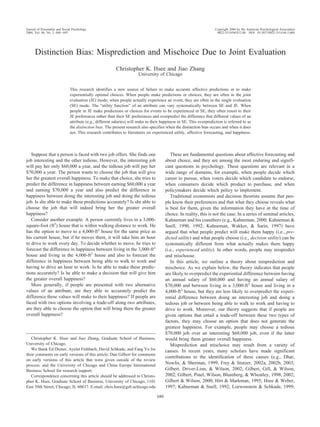
8. In Condition 3, the participants were not given a choice. They were
directly asked to recall and briefly write down a failure story and given a
15-g Dove chocolate to eat while performing the task. After they had
completed the task and eaten the chocolate, they were asked to indicate
their overall experience. After that, they were asked to indicate their
experience about the task and their experience about the chocolate sepa-
rately, as in Condition 1. All the responses were given on the same 9-point
scale as described above. Condition 4 was identical to Condition 3 except
that the respondents recalled and wrote down a success story and got only
a 5-g Dove chocolate.
Results
We report our results in two parts. We first report whether
choosers mispredicted the impact of the tasks and the impact of the
rewards. We then report whether choosers failed to make the
experientially optimal choice for themselves and for others.
Mispredictions. According to our theory regarding qualitative
and quantitative differences, we expected that choosers would not
overpredict the impact of the tasks but would overpredict the
impact of the chocolates, because the two tasks differed in valence,
and the two chocolates differed only in size.
We tested our predictions in two ways. First, we tested whether
choosers mispredicted others’ experiences. We did so by compar-
ing the predictions of the choosers in Condition 2, who made
predictions for others, with the experiences of the experiencers in
Conditions 3 and 4. Second, we tested whether choosers mispre-
dicted their own experiences with tasks and chocolates. We did so
by comparing the predictions of the choosers in Condition 1, who
made predictions for themselves, with their own subsequent expe-
riences. Figure 4 summarizes the results of the first comparison;
Figure 5 summarizes the results of the second comparison.
Both sets of results confirmed our predictions. As Figure 4
shows, choosers in Condition 2 did not overpredict the impact of
tasks on others’ experience. They predicted that experiencers
would be happier with the positive task than with the negative task
(M ⫽ 2.13 vs. –0.58), t(54) ⫽ 5.72, p ⬍ .001, and the experiencers
(those in Conditions 3 and 4) were indeed happier with the positive
task than with the negative task (M ⫽ 2.29 vs. –2.23), t(63) ⫽
11.86, p ⬍ .001. On the other hand, the choosers grossly overpre-
dicted the impact of the chocolates. They predicted that the larger
chocolate would engender greater happiness than the smaller choc-
olate (M ⫽ 2.67 vs. 0.47), t(54) ⫽ 6.69, p ⬍.001, but in reality the
larger chocolate did not bring any more happiness than the smaller
one (M ⫽ 1.65 vs. 1.94), t(63) ⬍ 1, ns.
Figure 5 shows a similar pattern. The choosers in Condition 1
predicted greater happiness with the positive task than with the
negative task (M ⫽ 2.17 vs. ⫺0.96), t(50) ⫽ 8.39, p ⬍ .001, and
indeed they were happier with the positive task than with the
negative task (M ⫽ 2.56 vs. –1.29), t(50) ⫽ 7.49, p ⬍ .001. On the
other hand, the choosers predicted greater happiness with the
bigger chocolate than with the smaller one (M ⫽ 2.31 vs. 1.02),
t(50) ⫽ 3.96, p ⬍ .001, but in reality the size of chocolate had no
significant effect (M ⫽ 1.75 vs. 1.11), t(50) ⫽ 1.15, ns.4
Mischoice. Because choosers overpredicted the impact of the
rewards but not the impact of the tasks, we expected a choice–
experience inconsistency in the following direction: The choosers
would favor the option with the larger reward, but the experiencers
would be happier with the option with the positive task.
Figure 6 summarizes the choice data. The left panel shows
results for those who chose for themselves (Condition 1). The right
panel shows results for those who chose for others (Condition 2).
Consistent with our prediction, the majority (65%) of the respon-
4
Unlike Conditions 3 and 4, in which the big and small chocolates made
no difference in experience, in Condition 1 the big and small chocolates
made some difference. This difference occurred perhaps because in Con-
dition 1 the experiencers had been the choosers themselves, had seen both
chocolates, and therefore were not in pure SE. This difference may also
have resulted from the fact that the experiencers had made predictions
during the choice phase, and their predictions may have influenced their
subsequent experiences (e.g., Sherman, 1980; Spangenberg & Greenwald,
1999).
Figure 4. Task–reward study: The left panel shows that choosers (for others) did not overpredict the difference
in others’ experience between doing the positive task and doing the negative task (which are qualitatively
different). The right panel shows that the choosers (for others) overpredicted the difference in others’ experience
between having the small reward and having the large reward (which are only quantitatively different).
687
DISTINCTION BIAS

9. dents in both conditions chose the negative-task/large-reward op-
tion, ␹2
(1, N ⫽ 55) ⫽ 5.25, p ⬍ .05, in both conditions.
Figure 7 summarizes the experience data. The left panel is the
result of those in Conditions 3 and 4 who did not make a choice
and therefore were experiencers in pure SE. The right panel is the
result of those in Condition 1, who had made a choice for them-
selves. In stark contrast with the preference revealed by the choice
data, both groups of experiencers were happier with the positive-
task/small-reward option than with the negative-task/large-reward
option: (M ⫽ 2.41 vs. –0.71), t(63) ⫽ 7.51, p ⬍ .001, for the pure
experiencers; (M ⫽ 2.61 vs. 0.09), t(50) ⫽ 5.61, p ⬍ .001, for the
choosers. The results in the right panel of Figure 7 are particularly
noteworthy. These are from people who had made the choice
themselves (Condition 1). In the choice phase, most of them opted
for the negative-task/large-reward option, but they ended up being
less happy than the minority of people who chose the positive-
task/small-reward option.5
Discussion
Study 3 may be a microcosm of life. In Study 3, most people
thought that the bigger chocolate would bring greater happiness
and chose to, or asked others to, endure a painful task in order to
obtain the bigger chocolate, yet the bigger chocolate did not bring
greater happiness. In real life, many people think that more money
would bring greater happiness and choose to, or encourage others
to, endure hard work in order to obtain more money, yet more
money may not bring more happiness. In this section, we discuss
the implications of Study 3 for misprediction and mischoice and
address several potential alternative explanations.
About mispredictions. The misprediction results secured in
this study replicate the misprediction results found in Studies 1 and
2. They show that people in JE are rather accurate in predicting the
impact of the difference between something good and something
bad but inaccurate in predicting the impact of the difference
between a small good thing and a large good thing. In other words,
the distinction bias occurs for merely quantitatively different val-
ues but not for qualitatively different values.
The misprediction results of this study also extend the previous
findings in one important direction: In the previous studies, the
predictors in JE were not told that the experiencers would be in
pure SE and might have thought that the experiencers would also
know the alternatives. Thus, what they were predicting may not
have been “how I would feel when I experience Option X if I
didn’t know about Option Y” but “how I would feel when I
experience Option X given that I also know about Option Y.” In
this study, the respondents in Condition 2 were asked to make
predictions for other people, and they were explicitly told that the
others would not know the alternative option, implying that the
experiencers were in pure SE. Even so, the predictors overpre-
dicted the impact of the rewards. In this sense, the misprediction
found in this study is more dramatic than that demonstrated in the
previous studies.
About mischoice. The study reveals two types of mischoices.
First, most people fail to choose the experientially optimal option
for others. Second, most people fail to choose the experientially
optimal option even for themselves. The first finding comes from
a comparison between the choices of those who made the choice
for others (Condition 2) and the experience of those who did not
choose (Conditions 3 and 4). This is a direct test of our theory. The
choosers (Condition 2) were in JE, and the experiencers (Condi-
tions 3 and 4) were in pure SE.
This finding has potentially important implications for the ex-
tensive economic literature on principals and agents. Agents make
decisions for principals. For example, lawyers (agents) make legal
decisions for their clients (principals); parents (agents) make mar-
ital decisions for their children (principals); policymakers (agents)
make policy decisions for their constituents (principals; e.g.,
5
Figure 7 reveals another potentially interesting effect: Compared with
the experiencers, the choosers seemed happier with the option they had
chosen, especially if they had chosen the negative-task/large-reward op-
tion. It suggests that people who made the choice themselves may have
experienced cognitive dissonance during the experience phase. Brown and
Feinberg (2002) have done extensive research on this topic.
Figure 5. Task–reward study: The left panel shows that choosers (for self) did not overpredict the difference
in their own subsequent experience between doing the positive task and doing the negative task. The right panel
shows that the choosers (for self) overpredicted the difference in their own subsequent experience between
having the small reward and having the large reward.
688 HSEE AND ZHANG

10. Shafir, 2002). The agents are the choosers; the principals are the
experiencers. Previous literature has identified various reasons
why agents may make poor choices: For example, they have
different tastes from the principals; they have ulterior motivations.
Our theory and data suggest that even if the agents are well
intended and have similar tastes to their principals, they may still
make poor choices, because the agents are usually in JE and the
principals are usually in SE.
In an article on fairness, Kahneman, Knetsch, and Thaler (1986)
made a similar point about consumers and theorists. They observed
that when consumers judge the fairness of an event, they rarely
compare it with other events, but when theorists study fairness,
they compare alternative scenarios. Consequently, theorists focus
too much on factors that seem salient in comparison but have little
influence on consumers’ fairness judgment.
The second finding—that people make suboptimal choices for
themselves—comes from a comparison between the choices of
people who made the choices for themselves and their own sub-
sequent experiences (Condition 1). This result is a less direct test
of our theory but is nevertheless intriguing. Here, the experiencers
were the choosers themselves, and they had already seen both
options when they experienced the chosen option. In this sense,
their experience was not in pure SE; they may have had some
memory of the foregone option. However, despite the possible
memory effect, the respondents were still happier with the
positive-task/small-reward option during the experience phase. It
suggests that experience is naturally an SE process.
We address a few potential alternative explanations here. First,
the choosers had not experienced the task or eaten the chocolate
when they made the choice, but the experiencers had done both
when they reported their experience and may have acquired more
knowledge or developed adaptation. To address this concern, we
asked the pure experiencers in Conditions 3 and 4 and the self-
choosers in Condition 1 to predict their overall experience right
before they started working on the task and eating the chocolate.
These are SE predictions. The results were similar to the SE–
experience results but in the opposite direction of the choice
results: For the pure experiencers, M ⫽ ⫺0.65 for the negative-
task/large-reward option, and M ⫽ 2.52 for the positive-task/
small-reward option; for the self-choosers, M ⫽ 0.24 for the
Figure 6. Task–reward study: Most choosers chose the negative-task/large-reward option over the positive-
task/small-reward option, regardless of whether they made the choice for themselves or for others (pure
experiencers).
Figure 7. Task–reward study: Both experiencers (who had not made choices) and choosers (who had made
choices) were happier with the positive task/small reward than with the negative task/large reward.
689
DISTINCTION BIAS

11. negative-task/large-reward option, and M ⫽ 2.44 for the positive-
task/small-reward option. These findings suggest that the choice–
experience inconsistency is not a result of differential knowledge
or adaptation.
Another potential alternative explanation for choice–experience
inconsistency is that the choosers based their decision on consid-
erations other than predicted happiness. This explanation implies
that the choosers could have accurately predicted that the positive-
task/small-reward option would provide better experience, yet for
other reasons they chose the negative-task/large-reward option. If
this explanation stands, then there should be an inconsistency
between what people predict will provide a better experience and
what people choose. To test this explanation, we ran another
condition (N ⫽ 33). It was similar to Condition 2 (choice for
others), except that the participants were asked to predict which
option would make the other participants happier. What we found
is that the prediction result was very similar to the choice result:
Most (66%) of the respondents predicted that the negative-task/
large-reward option would yield greater happiness than the
positive-task/small-reward option. Thus, the choice–experience
inconsistency in this study is chiefly a result of JE/SE mispredic-
tion, not a result of inconsistency between choice and predicted
experience.6
Other Evidence for Mischoice
Recently, we replicated the result of the task–reward study using
very different stimuli (Hsee & Zhang, 2003). The stimuli were two
audiovisual episodes. Each episode consisted of a static image and
a concurrent steady noise. The noise in the two episodes differed
only in degree of loudness, 72 dB and 78 dB, and the images in the
two episodes differed in quality, an ugly adult (in the softer noise
episode) and a cute baby (in the louder noise episode):
Noise Picture
Episode A 72 dB ugly adult
Episode B 78 dB cute baby
As in Study 3, participants in the study were assigned to one of
four conditions: choosers for self, choosers for others, pure expe-
riencers of the soft-noise/ugly-picture episode, and pure experi-
encers of the loud-noise/cute-picture episode. The choosers were
presented with samples from each episode and asked to compare
the samples before making a choice (JE). The pure experiencers
were presented with and experienced only one of the episodes
(SE).
Because the noises in the two episodes differed only quantita-
tively, and the images differed qualitatively, we expected the
noises to exert a greater impact on choice than on experience. The
results confirmed our expectation and are very similar to those in
Study 3. Both the choosers for self and the choosers for others
preferred the soft-noise/ugly-picture option, but both the pure
experiencers who had not seen both options and people who had
seen both options and made a choice for themselves were happier
with the loud-noise/cute-picture option.
This study was a strategic replication of Study 3. The two
studies used very different attributes: One used positive and neg-
ative life events, and one used pleasant and unpleasant pictures.
One used small and large chocolates, and one used loud and soft
noises. Despite these differences, the two studies revealed the
same pattern of choice–experience inconsistency.
General Discussion
When people predict the experiential impact of alternative val-
ues or choose between alternative options, they are in JE, but
people who eventually experience the value or the option are
usually in SE. The present research shows that JE and SE can lead
to systematically different results. Generally speaking, the utility
function of an attribute is flatter in SE than in JE, except around the
reference point. When people in JE make predictions or choices,
they do not spontaneously adjust for this difference; instead, they
project their preferences in JE onto their predictions and choices
for experiences in SE. As a result, they overweight differences that
seem distinct in JE but are actually inconsequential in SE.
The present research contributes to the existing affective fore-
casting literature by identifying evaluation mode as a source for
overprediction. Furthermore, our research not only accounts for
overprediction but also specifies when people do not overpredict.
Finally, our research extends the misprediction findings to some-
thing that has a behavioral consequence—mischoice.
In the remainder of the article, we first discuss the relationship
between the present research and several other lines of research we
recently conducted. Then we discuss ways to improve prediction
and reduce choice–experience inconsistency. Finally, we discuss
the implications of this work for research on subjective well-being.
Relationship With Evaluability
The JE/SE analysis we present in this article builds on the
evaluability hypothesis proposed by Hsee (1996, 1998, 2000) and
Hsee et al. (1999). In fact, the shape of the SE evaluation function
depicted in Figure 1 is adapted from Hsee et al. (1999). The
evaluability hypothesis was developed to explain preference re-
versals between JE and SE (e.g., Bazerman, Loewenstein, &
White, 1992; González-Vallejo & Moran, 2001; Hsee, 1996, 1998;
Kahneman, Ritov, & Schkade, 1999; Moore, 1999; Nowlis &
Simonson, 1997; Shafir, 2002; Sunstein, Kahneman, Schkade, &
Ritov, 2002). In a typical JE/SE reversal study reported by Hsee
(1996), for example, two job candidates for a computer-
programming position were evaluated in either JE or SE. The two
candidates involved a trade-off along two attributes—experience
in a special computer language and grade point average (GPA). In
JE, people were willing to pay more for the more experienced
candidate; but in SE, people were willing to pay more for the
higher GPA candidate. According to the evaluability hypothesis,
6
There may be another potential alternative explanation. Suppose that
most people prefer the negative-task/large-reward option but their prefer-
ence is very weak, and that a few people prefer the positive-task/small-
reward option and their preference is strong. Then most people would
choose the negative-task/large-reward option, but the mean experience
ratings may be higher for the other option. However, this explanation is not
likely for this study. First, there is no reason to believe that those who
prefer the negative-task/large-reward option have a weaker preference than
those who prefer the positive-task/small-reward option. Second, this ex-
planation is inconsistent with the finding that people in JE overpredicted
the impact of the reward but did not overpredict the impact of the tasks.
690 HSEE AND ZHANG

12. GPA is independently easier to evaluate for student respondents
than is programming experience. Thus, in SE, the respondents
based their judgment on GPA. In JE, the respondents could di-
rectly compare the two candidates’ experience levels. The com-
parison made the experience attribute easier to evaluate and hence
gave it more weight. (For information on other theories of prefer-
ence reversals, see, e.g., Fischer, Carmon, Ariely, & Zauberman,
1999; Irwin, 1994; Mellers, Chang, Birnbaum, & Ordóñez, 1992;
Nowlis & Simonson, 1997; Tversky, Sattath, & Slovic, 1988. For
a review, see Hsee, Zhang, & Chen, in press.)
The original evaluability hypothesis focuses on the difference
between independently easy-to-evaluate attributes and indepen-
dently difficult-to-evaluate attributes. The present research as-
sumes that most attributes are neither impossible to evaluate in-
dependently nor perfectly easy to evaluate independently. If an
attribute were impossible to evaluate independently, its SE curve
would be flat in all regions. If an attribute were perfectly easy to
evaluate independently, its SE curve would collapse with its JE
curve. For most attributes, which lie between these two extreme
cases, the SE curve is flatter than the JE curve in most regions,
except around the reference point. This is the case we depict in
Figure 1 and study in this article.
The present research extends the evaluability and JE/SE reversal
research in several important directions. First, the original evalu-
ability hypothesis posits that whether or not an attribute has a
greater impact on JE than on SE depends on whether the attribute
is independently difficult to evaluate. The present research shows
that whether or not an attribute has a greater impact on JE than on
SE depends on whether the values of the attribute under consid-
eration involve a quantitative difference or a qualitative difference.
As Study 1 and Study 2 show, even for the same attribute, values
in different regions could have either greater impact in JE than in
SE or similar impact between JE and SE, depending on whether
these values are quantitatively different or qualitatively different.
The concepts of quantitative/qualitative differences add greater
specificity and operationalism to the original evaluability
hypothesis.
Second, the original evaluability and JE/SE research was not
concerned about affective forecasting and did not ask respondents
in JE to predict their or other people’s feelings in SE. Therefore,
the responses of people in JE, though different from those of
people in SE, could not be considered biased. The present research
is concerned about affective forecasting and asks people in JE to
predict their or other people’s feelings in SE. Therefore, the
predictions of people in JE, which are different from the experi-
ences of people in SE, can be considered biased. This bias has not
been demonstrated in the original JE/SE literature.
Finally, the present research extends JE/SE reversal to choice–
experience inconsistency. We believe that choice–experience in-
consistency is a more important finding than a mere JE/SE rever-
sal. To appreciate this point, let us consider a distinction
Kahneman (1994) and others (see also Hammond, 1996; Sen,
1993; Hsee et al., in press) have drawn between internal inconsis-
tency and substantive inconsistency of decisions. Internal incon-
sistencies refer to findings that normatively inconsequential ma-
nipulations can change people’s preferences; they show that
preferences are labile. Substantive inconsistencies refer to findings
that people fail to choose what is best for them; they show that
decisions are suboptimal. The JE/SE reversal, as documented in
the existing literature, is an internal inconsistency. The choice–
experience inconsistency, as studied in the present research, is a
substantive inconsistency.
Relationship With Lay Rationalism and Medium
Maximization
So far, we have focused on distinction bias as the main cause of
choice–experience inconsistency. Here, we mention two other
related lines of research we recently conducted: lay rationalism
and medium maximization. Lay rationalism (Hsee, Zhang, et al.,
2003) refers to a tendency to overweight attributes that appear
rationalistic, such as quantity and economic value, and downplay
attributes that appear subjective. For example, when participants
were asked whether they would choose a small chocolate in the
shape of a heart or a large chocolate in the shape of a cockroach,
most opted for the large one. However, when asked which they
would enjoy more, most favored the small one.
Medium maximization (Hsee, Yu, et al., 2003) refers to a ten-
dency to focus on specious immediate payoffs rather than the
ultimate consequence of one’s action. For example, when partic-
ipants were asked to choose between a short task that would award
60 points and a long task that would award 100 points and told that
the points had no other use except that with 60 points they could
receive a vanilla ice cream and with 100 points they could receive
a pistachio ice cream (of equal amount), most chose the long task.
However, when asked which type of ice cream they preferred,
most favored the one corresponding to the short task (vanilla).
In theory, distinction bias is orthogonal to lay rationalism and
medium maximization. Distinction bias is about failure to make
accurate predictions and is a result of the JE/SE difference. Lay
rationalism and medium maximization are about failure to follow
predictions and are not due to the JE/SE difference. In reality,
however, these three factors can simultaneously lead to a choice–
experience inconsistency. For example, suppose that a person
chooses a tedious job that pays $70,000 a year over an interesting
job that pays $60,000 a year and that her long-term happiness
would actually be higher if she chose the lower paying job. Her
decision to choose the higher paying job may result from three
possible causes: First, she overpredicts the difference in happiness
between the two salaries—an example of distinction bias. Second,
she finds it more “rational” to base her choice on salary than on
interest—a manifestation of lay rationalism. Finally, she focuses
on the immediate payoff rather than the ultimate experiential
consequences of her choice—an instance of medium
maximization.
Ways to Improve Predictions and Decisions
The following story, from Hsee (2000), suggests a choice–
experience inconsistency due to the distinction bias and provides a
context in which to explore possible remedies. A person was
shopping for a pair of high-end speakers in an audio store. He was
particularly interested in one of two equally expensive models. He
found the appearance of one model very attractive and compatible
with his furniture and the appearance of the other model ugly and
incompatible with his furniture. A salesperson encouraged him to
compare the sound quality of the two models in a soundproof
audition room. Through careful comparisons he found the sound
691
DISTINCTION BIAS

13. quality of the ugly model slightly but distinctively better, and he
bought the ugly model. But soon after he had brought the speakers
home, he became so annoyed with their appearance that he rele-
gated these speakers to the basement.
This story implies a choice–experience inconsistency: The per-
son chose to buy the better sounding/ugly-looking model, but he
would probably have been happier had he bought the worse
sounding/good-looking model. This example also supports our
theory: The subtle difference in sound quality was only a matter of
degree and probably would make no difference in SE experience,
but the difference seemed distinct in JE and apparently dictated his
choice. This is a classic distinction bias.
How could we minimize the choice–experience inconsistency?
To reduce choice–experience inconsistency, choosers not only
need to predict their future experiences before making a choice but
also need to simulate SE in making predictions. The closer the
prediction is to SE, the more accurate it will be.
To illustrate, consider three possible ways the salesperson could
have asked the speaker buyer to predict his preference for two sets
of speakers:
1. The salesperson puts the two sets of speakers side by side and
allows the buyer to easily compare their sound with the push of a
button on a remote control. The salesperson asks the buyer, “Com-
pare them carefully. Which set do you enjoy more?” This method
is very similar to what the salesperson actually did in the example.
2. The same as above, except that the salesperson gives different
instructions: “Focus on one set of speakers first. Study it carefully
and think about how much you enjoy it. Write down your overall
impression. After that, focus on the other set. Study it carefully and
think about how much you enjoy it. Write down your overall
impression.”
3. The salesperson puts the two sets of speakers in different
rooms and prevents the buyer from making direct comparisons.
The salesperson first leads the buyer to one room and tells the
buyer, “Focus on this set of speakers. Study it carefully and think
about how much you enjoy it. Write down your overall impres-
sion.” The salesperson then sends the buyer away for a cup of tea.
Afterward, the salesperson leads the buyer to the other room and
repeats the procedure for the other pair of speakers.
Of the three cases, the first is closest to JE, and the last is closest
to SE. Specifically, in the first case, both the presentation of the
stimuli and the process of prediction are in JE. In the second case,
the presentation of the stimuli is still in JE, but the process of
prediction is closer to SE. In the last case, both the presentation of
the stimuli and the process of prediction are in SE.
We surmise that in the first case, the buyer is least likely to make
the correct prediction and least likely to choose the model that will
give him the best consumption experience and that in the last case,
he is most likely to do so. Unfortunately, the common practice is
much more similar to the first case than to the last case. Before
making decisions, people either spontaneously engage in, or are
encouraged by friends and professionals to engage in, direct com-
parisons of the choice alternatives. In fact, even decision experts
encourage people to do so (e.g., Janis & Mann, 1977). In stark
contrast with the traditional view, our advice is to refrain from
direct comparison. To make a good prediction and a good choice
for something that is to be consumed in SE, people should simulate
SE in prediction and in choice.
Of course, we do not mean that people should always avoid JE
during choice. Instead, we mean that people should align the
evaluation mode of choice with the evaluation mode of consump-
tion. Thus, if the consumption will take place in JE, people should
engage in JE in choice. For example, suppose that a person is
buying a dress that she will wear to a party, where people will
naturally compare each others’ dresses. Then she should engage in
JE when she makes her purchase decision. If she does not engage
in JE and instead she decides whether to buy a particular dress
based on how good the dress looks by itself rather than how good
the dress looks in comparison with other dresses, then she may fail
to buy the dress that would give her the greatest happiness at the
party.
Another situation in which one should conduct JE in choice is
when the objective of the choice is to maximize some other value
than consumption experience, and JE is more likely than SE to
identify the option that would maximize that value. For example,
suppose that a person working in the admissions office of a college
wants to recruit students who have the greatest academic potential.
In this case, JE of all applicants is more likely than SE to identify
such students, and the person should adopt JE. Generally speaking,
if the purpose of one’s decision is to maximize consumption
experience, and the consumption will take place in SE, then the
decision maker should simulate SE when making the decision.
Implications for Happiness Research
For most people, the pursuit of subjective well-being, or broadly
defined happiness, is an ultimate goal of life. In recent years, both
psychologists and economists have made significant contributions
to the understanding of happiness (e.g., Argyle, 1987; Diener,
2000; Diener, Scollon, & Lucas, in press; Diener, Suh, Lucas, &
Smith, 1999; Diener, Tamir, Kim-Prieto, Scollon, & Diener, 2003;
Easterlin, 1974, 2001; Frank, 1997; Frey & Stutzer, 2000, 2002a,
2002b; Kahneman, 2000; Kahneman, Diener, & Schwarz, 1999;
Myers, 1993; Ryan & Deci, 2001; Scitovsky, 1976; Seligman,
2002; Seligman & Csikszentmihalyi, 2000; Strack, Argyle, &
Schwarz, 1991).
Among other things, the literature has documented three robust
findings: First, virtually everyone prefers more money to less
money. Second, across generations, when individuals’ wealth has
steadily increased, happiness has not. Finally, at a given time in a
given society, wealthy people are happier than less wealthy people,
but the correlation is small. These findings, especially the latter
two, have received various explanations, including adaptation and
rising aspirations (e.g., Brickman, Coates, & Janoff-Bulman, 1978;
Diener et al., 1999, 2003; Easterlin, 2001; Frederick & Loewen-
stein, 1999; van Praag, 2003).
We offer an additional, and not necessarily alternative, expla-
nation for these findings. First, why do people prefer more money
to less money? When choosing whether to have more or less
wealth, they are in JE of different wealth scenarios, and so their
evaluation curve resembles the generally steeper JE curve in
Figure 1. More wealth is obviously better.
Second, why has happiness not increased across generations
when wealth has? For example, why is the happiness of the
average person in the 1990s similar to the happiness of the average
person in the 1970s, even though the person in the 1990s possesses
more wealth than the person in the 1970s? According to our
692 HSEE AND ZHANG

14. theory, when people report their happiness, they are mostly in SE
of their states, including their financial states, and they do not
spontaneously compare across generations. Thus, the wealth-to-
happiness function resembles our SE curve in Figure 1. Except at
very low wealth levels, the evaluation curve is largely flat. (Even
if some people do compare their wealth with the wealth of a
previous generation, this effect will be a constant and will not
make a later generation happier than a previous generation. For
example, suppose that some people in the 1990s compared their
wealth with that of people in the 1970s and felt happy. Then some
people in the 1970s would also have compared their wealth with
that of people in the 1950s and also felt happy. Such comparisons,
if any, would not make people in the 1990s happier than people in
the 1970s.)
Finally, why at a given time in a given society are wealthy
people somewhat happier than less wealthy people? That is be-
cause at a given time within a given society people may occasion-
ally compare themselves with each other, and therefore their
happiness has an element of JE. (For example, people may say, “I
feel awful, because my neighbor recently bought a global posi-
tioning system for his new Jaguar, but I do not even have enough
money to fix the muffler of my old Dodge.”) However, we believe
that in most situations, people do not engage in such comparisons;
instead, they mostly mind their own states and experience their
own lives as in SE. This probably is why, even at a given time and
within a given society, the correlation between wealth and happi-
ness is rather small.
In a recent article, van Praag (2003) made an insightful distinc-
tion between a virtual welfare (happiness) function and a true
welfare (happiness) function. The virtual welfare function repre-
sents people’s evaluations of different fictitious income levels. The
true welfare function represents people’s evaluations of their own
income levels. According to van Praag, the virtual welfare function
is generally steeper than the true welfare function. This proposition
is consistent with ours. In our terms, the virtual welfare function
represents JE of alternative income levels and resembles the
steeper JE curve in Figure 1, and the true welfare function repre-
sents SE of people’s own incomes and therefore resembles the
flatter SE curve in Figure 1. van Praag made another important
argument: The virtual welfare function reflects how individuals
evaluate different income levels when making a decision and
describes the decision utility of incomes. In contrast, the true
welfare function reflects how individuals experience their incomes
in reality and describes the experienced utility of incomes. This
analysis corroborates our assertion that decisions are based on JE
of alternative scenarios, and experiences reflect SE of actual
outcomes.
Happiness researchers have also tried to determine what factors
affect happiness and what factors do not. For example, Easterlin
(2003) recently observed that factors such as whether a person is
in good or poor health and whether a person is married or widowed
have greater effects on happiness than material factors such as
income and home size (see also Frey & Stutzer, 2003; McLanahan
& Sorensen, 1984; Myers, 1993). These effects may be multiply
determined. One likely explanation is differential adaptation: It is
more difficult to adapt to poor health or widowhood than to wealth
(Easterlin, 2003). Another potential explanation is our analysis on
qualitative and quantitative differences. Differences such as
whether a person is in good or poor health and whether a person is
married or divorced are qualitative and have significant impact on
happiness. On the other hand, differences such as whether a person
earns $60,000 or $70,000 a year and whether a person lives in a
3,000- or 4,000-ft2
home—as long as these differences do not
cross a reference point—are merely quantitative and have less
impact on happiness. More importantly, our theory suggests that in
making decisions, people are more likely to overestimate the
impact of factors such as income and home size than to overesti-
mate the impact of factors such as health and marriage. We hope
that our theory can help people make better predictions and hap-
pier choices.
References
Amir, O., & Ariely, D. (2003). Decision by rules: Disassociation between
preferences and willingness to act. Unpublished manuscript.
Argyle, M. (1987). The psychology of happiness. London: Methuen.
Bazerman, M. H., Loewenstein, G., & White, S. B. (1992). Reversals of
preference in allocation choices: Judging an alternative versus choosing
among alternatives. Administrative Science Quarterly, 37, 220–240.
Brickman, P., Coates, D., & Janoff-Bulman, R. (1978). Lottery winners
and accident victims: Is happiness relative? Journal of Personality and
Social Psychology, 36, 917–927.
Brown, C., & Feinberg, F. (2002). How does choice affect evaluations?
Advances in Consumer Research, 29, 331–332.
Dhar, R., Nowlis, S. M., & Sherman, S. J. (1999). Comparison effects on
preference construction. Journal of Consumer Research, 26, 293–306.
Diener, E. (2000). Subjective well-being: The science of happiness and a
proposal for a national index. American Psychologist, 55, 34–43.
Diener, E., Scollon, C. N., & Lucas, R. E. (in press). The evolving concept
of subjective well-being: The multifaceted nature of happiness. In P. T.
Costa & I. C. Siegler (Eds.), The psychology of aging. New York:
Elsevier Science.
Diener, E., Suh, E. M., Lucas, R. E., & Smith, H. L. (1999). Subjective
well-being: Three decades of progress. Psychological Bulletin, 125,
276–302.
Diener, E., Tamir, M., Kim-Prieto, C., Scollon, C. N., & Diener, M. (2003).
A time-sequential framework for understanding subjective well-being
and ill-being. Unpublished manuscript.
Dunn, E. W., Wilson, T. D., & Gilbert, D. T. (2003). Location, location,
location: The misprediction of satisfaction in housing lotteries. Person-
ality and Social Psychology Bulletin, 29, 1421–1432.
Easterlin, R. A. (1974). Does economic growth improve the human lot? In
P. A. David & M. W. Reder (Eds.), Nations and households in economic
growth: Essays in honor of Moses Abramovitz (pp. 89–125). New York:
Academic Press.
Easterlin, R. A. (2001). Income and happiness: Towards a unified theory.
The Economic Journal, 111, 465–484.
Easterlin, R. A. (2003). Building a better theory of well-being [IZA
discussion paper]. Bonn, Germany: Institute for the Study of Labor.
Fischer, G. W., Carmon, Z., Ariely, D., & Zauberman, G. (1999). Goal-
based construction of preferences: Task goals and the prominence effect.
Management Science, 45, 1057–1075.
Frank, R. H. (1997). The frame of reference as a public good. Economic
Journal, 107, 1832–1847.
Frederick, S., & Loewenstein, G. (1999). Hedonic adaptation. In D. Kah-
neman, E. Diener, & N. Schwarz (Eds.), Well-being: The foundations of
hedonic psychology. New York: Russell Sage Foundation.
Frey, B. S., & Stutzer, A. (2000). Happiness, economy and institutions.
Economic Journal, 110, 918–938.
Frey, B. S., & Stutzer, A. (2002a). Happiness and economics. Princeton,
NJ: Princeton University Press.
Frey, B. S., & Stutzer, A. (2002b). What can economists learn from
happiness research? Journal of Economic Literature, 40, 402–435.
693
DISTINCTION BIAS

15. Frey, B. S., & Stutzer, A. (2003). Economic consequences of mispredicting
utility. Unpublished manuscript.
Gilbert, D. T., Driver-Linn, E., & Wilson, T. D. (2002). The trouble with
Vronsky: Impact bias in the forecasting of future affective states. In L. F.
Barrett & P. Salovey (Eds.), The wisdom in feeling: Psychological
processes in emotional intelligence (pp. 114–143). New York: Guilford
Press.
Gilbert, D. T., Gill, M., & Wilson, T. D. (2002). The future is now:
Temporal correction in affective forecasting. Organizational Behavior
and Human Decision Processes, 88, 430–444.
Gilbert, D. T., Pinel, E. C., Wilson, T. D., Blumberg, S. J., & Wheatley, T.
(1998). Immune neglect: A source of durability bias in affective fore-
casting. Journal of Personality and Social Psychology, 75, 617–638.
Gilbert, D. T., Pinel, E. C., Wilson, T. D., Blumberg, S. J., & Wheatley,
T. P. (2002). Durability bias in affective forecasting. In T. Gilovich, D.
Griffin, & D. Kahneman (Eds.), Heuristics and biases: The psychology
of intuitive judgment (pp. 292–312). Cambridge, England: Cambridge
University Press.
Gilbert, D. T., & Wilson, T. D. (2000). Miswanting: Some problems in the
forecasting of future affective states. In J. Forgas (Ed.), Feeling and
thinking: The role of affect in social cognition (pp. 178–197). Cam-
bridge, England: Cambridge University Press.
González-Vallejo, C., & Moran, E. (2001). The evaluability hypothesis
revisited: Joint and separate evaluation preference reversal as a function
of attribute importance. Organizational Behavior and Human Choice
Processes, 86, 216–233.
Hammond, K. R. (1996). How convergence of research paradigms can
improve research on diagnostic judgment. Medical Decision Making, 16,
281–287.
Hirt, E. R., & Markman, K. D. (1995). Multiple explanations: A consider-
an-alternative strategy for debiasing judgments. Journal of Personality
and Social Psychology, 69, 1069–1086.
Houston, D. A., & Sherman, S. J. (1995). Cancellation and focus: The role
of shared and unique features in the choice process. Journal of Exper-
imental Social Psychology, 31, 357–378.
Hsee, C. K. (1996). The evaluability hypothesis: An explanation of pref-
erence reversals between joint and separate evaluations of alternatives.
Organizational Behavior and Human Choice Processes, 46, 247–257.
Hsee, C. K. (1998). Less is better: When low-value options are judged
more highly than high-value options. Journal of Behavioral Decision
Making, 11, 107–121.
Hsee, C. K. (2000). Attribute evaluability and its implications for joint–
separate evaluation reversals and beyond. In D. Kahneman & A. Tversky
(Eds.), Choices, values and frames (pp. 543–563). Cambridge, England:
Cambridge University Press.
Hsee, C. K., & Leclerc, F. (1998). Will products look more attractive when
evaluated jointly or when evaluated separately? Journal of Consumer
Research, 25, 175–186.
Hsee, C. K., Loewenstein, G., Blount, S., & Bazerman, M. H. (1999).
Preference reversals between joint and separate evaluations of options:
A review and theoretical analysis. Psychological Bulletin, 125, 576–
591.
Hsee, C. K., & Rottenstreich, Y. (2004). Music, pandas, and muggers: On
the affective psychology of value. Journal of Experimental Psychology:
General, 133, 23–30.
Hsee, C. K., & Weber, E. U. (1997). A fundamental prediction error:
Self–other discrepancies in risk preference. Journal of Experimental
Psychology: General, 126, 45–53.
Hsee, C. K., Yu, F., Zhang, J., & Zhang, Y. (2003). Medium maximization.
Journal of Consumer Research, 30, 1–14.
Hsee, C. K., & Zhang, J. (2003). Inconsistency between choice and
consumption experience. Unpublished manuscript.
Hsee, C. K., Zhang, J., & Chen, J. (in press). Internal and substantive
inconsistencies in decision-making. In D. J. Koehler & N. Harvey (Eds.),
Blackwell handbook of judgment and decision making. Oxford, England:
Blackwell.
Hsee, C. K., Zhang, J., Yu, F., & Xi, Y. (2003). Lay rationalism and
inconsistency between predicted experience and decision. Journal of
Behavioral Decision Making, 16, 257–272.
Irwin, J. R. (1994). Buying/selling price preference reversals: Preference
for environmental changes in buying versus selling modes. Organiza-
tional Behavior and Human Choice Processes, 60, 431–457.
Janis, I. L., & Mann, L. (1977). Choice making: A psychological analysis
of conflict, choice, and commitment. New York: Free Press.
Kahneman, D. (1994). New challenges to the rationality assumption.
Journal of Institutional and Theoretical Economics, 150, 18–36.
Kahneman, D. (1995). Varieties of counterfactual thinking. In N. J. Roese
& J. M. Olson (Eds.), What might have been: The social psychology of
counterfactual thinking (pp. 375–396). Mahwah, NJ: Erlbaum.
Kahneman, D. (2000). Experienced utility and objective happiness: A
moment-based approach. In D. Kahneman & A. Tversky (Eds.),
Choices, values and frames (pp. 673–692). Cambridge, England: Cam-
bridge University Press.
Kahneman, D., Diener, E., & Schwarz, N. (Eds.). (1999). Well-being: The
foundations of hedonic psychology. New York: Russell Sage
Foundation.
Kahneman, D., Knetsch, J. L., & Thaler, R. H. (1986). Fairness and the
assumptions of economics. Journal of Business, 59, 285–300.
Kahneman, D., Ritov, I., & Schkade, D. (1999). Economic preferences or
attitude expressions? An analysis of dollar responses to public issues.
Journal of Risk and Uncertainty, 19, 203–235.
Kahneman, D., & Snell, J. (1990). Predicting utility. In R. M. Hogarth
(Ed.), Insights in decision making (pp. 295–310). Chicago: University of
Chicago Press.
Kahneman, D., & Snell, J. S. (1992). Predicting a changing taste: Do
people know what they will like? Journal of Behavioral Decision
Making, 5, 187–200.
Kahneman, D., & Tversky, A. (1979). Prospect theory: An analysis of
decision under risk. Econometrica, 47, 263–292.
Kahneman, D., & Tversky, A. (1982). The simulation heuristic. In D.
Kahneman, P. Slovic, & A. Tversky (Eds.), Judgment under uncertainty:
Heuristics and biases (pp. 201–208). New York: Cambridge University
Press.
Kahneman, D., Wakker, P. P., & Sarin, R. (1997). Back to Bentham?
Explorations of experienced utility. Quarterly Journal of Economics,
112, 1937–1996.
Kleinmuntz, D. N., & Schkade, D. (1993). Information displays and
decision processes. Psychological Science, 4, 221–227.
Loewenstein, G. (1996). Out of control: Visceral influences on behavior.
Organizational Behavior and Human Choice Processes, 65, 272–292.
Loewenstein, G., & Schkade, D. (1999). Wouldn’t it be nice? Predicting
future feelings. In D. Kahneman, E. Diener, & N. Schwarz (Eds.),
Well-being: The foundations of hedonic psychology (pp. 85–105). New
York: Russell Sage Foundation.
March, J. (1994). A primer on decision making: How decisions happen.
New York: Free Press.
Markman, K. D., & Hirt, E. R. (2002). Social prediction and the allegiance
bias. Social Cognition, 20, 58–86.
McLanahan, S. S., & Sorensen, A. B. (1984). Life events and psycholog-
ical well-being: A reexamination of theoretical and methodological
issues. Social Science Research, 13, 111–128.
Mellers, B. A., Chang, S., Birnbaum, M. H., & Ordóñez, L. D. (1992).
Preferences, prices, and ratings in risky decision making. Journal of
Experimental Psychology: Human Processes and Performance, 18,
347–361.
Moore, D. (1999). Order effects in preference judgments: Evidence for
context dependence in the generation of preferences. Organizational
Behavior and Human Choice Processes, 78, 146–165.
694 HSEE AND ZHANG

16. Myers, D. G. (1993). The pursuit of happiness: Who is happy and why?
New York: Avon Books.
Novemsky, N., & Ratner, R. K. (2003). The time course and impact of
consumers’ erroneous beliefs about hedonic contrast effects. Journal of
Consumer Research, 29, 507–516.
Nowlis, S. M., & Simonson, I. (1997). Attribute-task compatibility as a
determinant of experiencer preference reversals. Journal of Marketing
Research, 34, 205–218.
Prelec, D., & Herrnstein, R. (1993). Preferences or principles: Alternative
guidelines for choice. In R. J. Zeckhauser (Ed.), Strategy and choice (pp.
319–340). Cambridge, MA: MIT Press.
Ratner, R. K., Kahn, B., & Kahneman, D. (1999). Choosing less-preferred
experiences for the sake of variety. Journal of Consumer Research, 26,
1–15.
Read, D., & van Leeuwen, B. (1998). Predicting hunger: The effects of
appetite and delay on choice. Organizational Behavior and Human
Decision Processes, 76, 189–205.
Roese, N. J. (1997). Counterfactual thinking. Psychological Bulletin, 121,
133–148.
Ryan, R. M., & Deci, E. L. (2001). On happiness and human potentials: A
review of research on hedonic and eudaimonic well-being. Annual
Review of Psychology, 52, 141–166.
Schkade, D. A., & Kahneman, D. (1998). Does living in California make
people happy? A focusing illusion in judgments of life satisfaction.
Psychological Science, 9, 340–346.
Scitovsky, T. (1976). The joyless economy: An inquiry into human satis-
faction and dissatisfaction. New York: Oxford University Press.
Seligman, M. E. P. (2002). Authentic happiness: Using the new positive
psychology to realize the potential for lasting fulfillment. New York:
Free Press.
Seligman, M. E. P., & Csikszentmihalyi, M. (2000). Positive psychology:
An introduction. American Psychologist, 55, 5–14.
Sen, A. (1993). Internal consistency of choice. Econometrica, 61, 495–521.
Shafir, E. (2002). Cognition, intuition and policy guidelines. In R. Gowda
& J. Fox (Eds.), Judgments, choices, and public policy (pp. 71–88).
Cambridge, England: Cambridge University Press.
Sherman, S. J. (1980). On the self-erasing nature of errors of prediction.
Journal of Personality and Social Psychology, 39, 211–221.
Simonson, I. (1990). The effect of purchase quantity and timing on variety-
seeking behavior. Journal of Marketing Research, 27, 150–162.
Simonson, I., & Nowlis, S. M. (2000). The role of explanations and need
for uniqueness in consumer decision making: Unconventional choices
based on reasons. Journal of Consumer Research, 27, 49–68.
Spangenberg, E. R., & Greenwald, A. G. (1999). Social influence by
requesting self-prophecy. Journal of Consumer Psychology, 8, 61–89.
Strack, F., Argyle, M., & Schwarz, N. (Eds.). (1991). Subjective well-
being: An interdisciplinary perspective. New York: Pergamon Press.
Sunstein, C. R., Kahneman, D., Schkade, D., & Ritov, I. (2002). Predict-
ably incoherent judgments. Stanford Law Review, 54, 1153–1215.
Tversky, A. (1969). Intransitivity of preferences. Psychological Review,
76, 31–48.
Tversky, A., Sattath, S., & Slovic, P. (1988). Contingent weighting in
judgment and choice. Psychological Review, 95, 371–384.
van Praag, B. M. S. (2003). The connection between old and new ap-
proaches to financial satisfaction. Unpublished manuscript.
Willemsen, M. C., & Keren, G. (2002). Negative-based prominence: The
role of negative features on matching and choice. Organizational Be-
havior and Human Decision Processes, 88, 643–666.
Willemsen, M. C., & Keren, G. (in press). The role of negative features in
joint and separate evaluation. Journal of Behavioral Decision Making.
Wilson, T. D., & Gilbert, D. T. (2003). Affective forecasting. In M. Zanna
(Ed.), Advances in experimental social psychology (pp. 345–411). New
York: Elsevier.
Wilson, T. D., Kraft, D., & Dunn, D. S. (1989). The disruptive effects of
explaining attitudes: The moderating effect of knowledge about the
attitude object. Journal of Experimental Social Psychology, 25, 379–
400.
Wilson, T. D., & Schooler, J. (1991). Thinking too much: Introspection can
reduce the quality of preferences and choices. Journal of Personality and
Social Psychology, 60, 181–192.
Wilson, T. D., Wheatley, T., Meyers, J. M., Gilbert, D. T., & Axsom, D.
(2000). Focalism: A source of durability bias in affective forecasting.
Journal of Personality and Social Psychology, 78, 821–836.
Received July 30, 2003
Revision received January 13, 2004
Accepted January 13, 2004 䡲
695
DISTINCTION BIAS