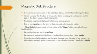
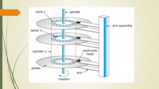
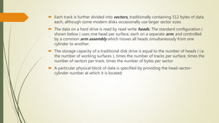
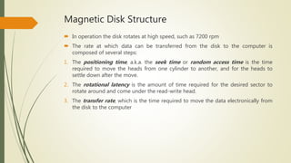
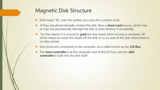
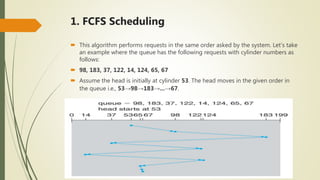
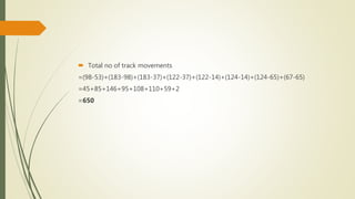
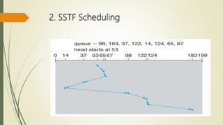
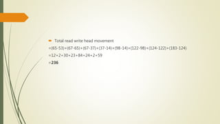
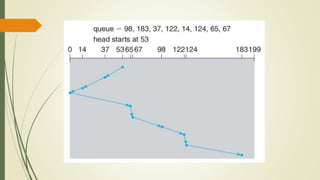
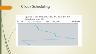
The document discusses secondary storage and magnetic disk structure. It provides details on: - Secondary storage devices like disks, tapes, and drives have non-volatile memory and are slower but cheaper than primary storage like RAM. - Magnetic disks are divided into platters, tracks, cylinders, and sectors. Read/write heads access data locations specified by head, sector, cylinder addresses. - Various disk scheduling algorithms like FCFS, SSTF, SCAN, C-SCAN, and LOOK are described which improve disk bandwidth and access time by processing requests in different orders.

1. Secondary Storage
:Disk structure
Prepared By: Mr. Sangram A. Patil
Assistant Professor PVPIT,Budhgaon

2. Secondary Storage
 Secondary storage devices are those devices whose memory is non volatile
 Secondary storage is also called auxiliary storage.
 Secondary storage is less expensive as compared to primary memory like RAMs.
 The speed of the secondary storage is also lesser than that of primary storage.
 Hence, the data which is less frequently accessed is kept in the secondary storage.
 A few examples are magnetic disks, magnetic tapes, removable thumb drives etc.

3. Magnetic Disk Structure
 In modern computers, most of the secondary storage is in the form of magnetic disks.
 Hence, knowing the structure of a magnetic disk is necessary to understand how the
data in the disk is accessed by the computer.
 Traditional magnetic disks have the following basic structure:
 One or more platters in the form of disks covered with magnetic media.
Hard disk platters are made of rigid metal, while "floppy" disks are made of more
flexible plastic.
 Each platter has two working surfaces.
 Each working surface is divided into a number of concentric rings called tracks.
 The collection of all tracks that are the same distance from the edge of the platter, ( i.e.
all tracks immediately above one another in the following diagram ) is called a cylinder.

5.  Each track is further divided into sectors, traditionally containing 512 bytes of data
each, although some modern disks occasionally use larger sector sizes.
 The data on a hard drive is read by read-write heads. The standard configuration (
shown below ) uses one head per surface, each on a separate arm, and controlled
by a common arm assembly which moves all heads simultaneously from one
cylinder to another.
 The storage capacity of a traditional disk drive is equal to the number of heads ( i.e.
the number of working surfaces ), times the number of tracks per surface, times the
number of sectors per track, times the number of bytes per sector.
 A particular physical block of data is specified by providing the head-sector-
cylinder number at which it is located.

6. Magnetic Disk Structure
 In operation the disk rotates at high speed, such as 7200 rpm
 The rate at which data can be transferred from the disk to the computer is
composed of several steps:
1. The positioning time, a.k.a. the seek time or random access time is the time
required to move the heads from one cylinder to another, and for the heads to
settle down after the move.
2. The rotational latency is the amount of time required for the desired sector to
rotate around and come under the read-write head.
3. The transfer rate, which is the time required to move the data electronically from
the disk to the computer

7. Magnetic Disk Structure
 Disk heads "fly" over the surface on a very thin cushion of air.
 If they should accidentally contact the disk, then a head crash occurs, which may
or may not permanently damage the disk or even destroy it completely.
 For this reason it is normal to park the disk heads when turning a computer off,
which means to move the heads off the disk or to an area of the disk where there is
no data stored.
 Disk drives are connected to the computer via a cable known as the I/O Bus.
 The host controller is at the computer end of the I/O bus, and the disk
controller is built into the disk itself

8. Disk Scheduling
 Disk transfer speeds are limited primarily by seek times and rotational
latency. When multiple requests are to be processed there is also some inherent
delay in waiting for other requests to be processed.
 Bandwidth is measured by the amount of data transferred divided by the total
amount of time from the first request being made to the last transfer being
completed.
 Both bandwidth and access time can be improved by processing requests in a
good order.
 Disk requests include the disk address, memory address, number of sectors to
transfer, and whether the request is for reading or writing.

9. 1. FCFS Scheduling
 This algorithm performs requests in the same order asked by the system. Let's take
an example where the queue has the following requests with cylinder numbers as
follows:
 98, 183, 37, 122, 14, 124, 65, 67
 Assume the head is initially at cylinder 53. The head moves in the given order in
the queue i.e., 53→98→183→...→67.

10.  Total no of track movements
=(98-53)+(183-98)+(183-37)+(122-37)+(122-14)+(124-14)+(124-65)+(67-65)
=45+85+146+95+108+110+59+2
=650

11. 2. SSTF Scheduling
 Here the position which is closest to the current head position is chosen first.
Consider the previous example where disk queue looks like,
98, 183, 37, 122, 14, 124, 65, 67
 Assume the head is initially at cylinder 53. The next closest cylinder to 53 is 65,
and then the next nearest one is 67, then 37, 14, so on.
 Shortest Seek Time First scheduling is more efficient, but may lead to starvation if
a constant stream of requests arrives for the same general area of the disk.

12. 2. SSTF Scheduling

13.  Total read write head movement
=(65-53)+(67-65)+(67-37)+(37-14)+(98-14)+(122-98)+(124-122)+(183-124)
=12+2+30+23+84+24+2+59
=236

14. 3. SCAN Scheduling
 This algorithm is also called the elevator algorithm because of it's behavior. Here,
first the head moves in a direction (say backward) and covers all the requests in the
path. Then it moves in the opposite direction and covers the remaining requests in
the path. This behavior is similar to that of an elevator. Let's take the previous
example,
 98, 183, 37, 122, 14, 124, 65, 67
 Assume the head is initially at cylinder 53. The head moves in backward direction
and accesses 37 and 14. Then it goes in the opposite direction and accesses the
cylinders as they come in the path.

16.  Total read write head movement
=(53-0)+(183-0)
=236

17. 4. C-SCAN Scheduling
 The Circular-SCAN algorithm improves upon SCAN by treating all requests in a
circular queue fashion - Once the head reaches the end of the disk, it returns to
the other end without processing any requests, and then starts again from the
beginning of the disk:

18.  Total read write head movement
=(199-53)+(199-0)+(37-0)
=146+199+37
=382

19. 5 LOOK Scheduling
 LOOK scheduling improves upon SCAN by looking ahead at the queue of
pending requests, and not moving the heads any farther towards the end of the
disk than is necessary. The following diagram illustrates the circular form of
LOOK:

20.  Total read write head movement
=(183-53)+(183-14)
=130+169
=299

21. C look Scheduling