Os(18 cs43) module5

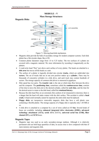
Operating Systems (18CS43)
Prof. S. V. Manjaragi, Dept. of CSE, Hirasugar Institute of Technology, Nidasoshi Page 1
Magnetic Disks
-
MODULE – V
Mass Storage Structures
Figure 7.1 Moving-head disk mechanism.
 Magnetic disks provide the bulk of secondary storage for modern computer systems. Each disk
platter has a flat circular shape, like a CD.
 Common platter diameters range from 1.8 to 5.25 inches. The two surfaces of a platter are
covered with a magnetic material. We store information by recording it magnetically on the
platters.
 A read-write head "flies" just above each surface of every platter. The heads are attached to a
disk arm that moves all the heads as a unit.
 The surface of a platter is logically divided into circular tracks, which are subdivided into
sectors. The set of tracks that are at one arm position makes up a cylinder. There may be
thousands of concentric cylinders in a disk drive, and each track may contain hundreds of
sectors. The storage capacity of common disk drives is measured in gigabytes.
 Disk speed has two parts. The transfer rate is the rate at which data flow between the drive
and the computer. The positioning time, sometimes called the random-access time, consists
of the time to move the disk arm to the desired cylinder, called the seek time, and the time for
the desired sector to rotate to the disk head, called the rotational latency.
 Because the disk head flies on an extremely thin cushion of air (measured in microns), there is
a danger that the head will make contact with the disk surface. This accident is called a head
crash. A head crash normally cannot be repaired; the entire disk must be replaced.
 Floppy disks are inexpensive removable magnetic disks that have a soft plastic case
containing a flexible platter. The storage capacity of a floppy disk is typically only 1.44 MB or
so.
 A disk drive is attached to a computer by a set of wires called an I/O bus. Several kinds of
buses are available, including enhanced integrated drive electronics (EIDE), advanced
technology attachment (ATA), serial ATA (SATA), universal serial bus (USB), fiber
channel (FC), and SCSI buses.
Magnetic Tapes
 Magnetic tape was used as an early secondary-storage medium. Although it is relatively
permanent and can hold large quantities of data, its access time is slow compared with that of
main memory and magnetic disk.

 Tapes are used mainly for backup, for storage of infrequently used information, and as a
medium for transferring information from one system to another.
 Tape capacities vary greatly, depending on the particular kind of tape drive. Typically, they
store from 20 GB to 200 GB.
 Some have built-in compression that can more than double the effective storage. Tapes and
their drivers are usually categorized by width, including 4, 8, and 19 millimeters and 1/4 and
1/2 inch.
Disk Scheduling
 One of the responsibilities of the operating system is to use the hardware efficiently. For the
disk drives, meeting this responsibility entails having fast access time and large disk
bandwidth.
 The access time has two major components. The seek time is the time for the disk arm to move
the heads to the cylinder containing the desired sector. The rotational latency is the additional
time for the disk to rotate the desired sector to the disk head.
 Whenever a process needs I/O to or from the disk, it issues a system call to the operating
system. The request specifies several pieces of information:
• Whether this operation is input or output
• What the disk address for the transfer is
• What the memory address for the transfer is
• What the number of sectors to be transferred is
 If the desired disk drive and controller are available, the request can be serviced immediately.
If the drive or controller is busy, any new requests for service will be placed in the queue of
pending requests for that drive.
FCFS (First Come First Serve) Scheduling
 The simplest form of disk scheduling is, of course, the first-come, first-served (FCFS)
algorithm.
 This algorithm is intrinsically fair, but it generally does not provide the fastest service.
 Consider, for example, a disk queue with requests for I/O to blocks on cylinders 98, 183,
37,122, 14, 124, 65, 67 in that order.
 If the disk head is initially at cylinder 53, it will first move from 53 to 98, then to 183, 37, 122,
14, 124/65, and finally to 67, for a total head movement of 640 cylinders.
 This schedule is diagrammed in Figure 7.2.
Figure 7.2FCFS disk scheduling.

Average Seek Length = Total no. of Moves/No. of requests
= 644 / 8 = 80.5
SSTF (Shortest Seek Time First) Scheduling
 It seems reasonable to service all the requests close to the current head position before moving
the head far away to service other requests. This assumption is the basis for the shortest-seek-
time-first (SSTF) algorithm.
 The SSTF algorithm selects the request with the minimum seek time from the current head
position. Since seek time increases with the number of cylinders traversed by the head, SSTF
chooses the pending request closest to the current head position.
 Consider, for example, a disk queue with requests for I/O to blocks on cylinders 98, 183,
37,122, 14, 124, 65, 67 in that order. For this example, the closest request to the initial head
position (53) is at cylinder 65. Once we are at cylinder 65, the next closest request is at
cylinder 67. From there, the request at cylinder 37 is closer than the one at 98, so 37 is served
next. Continuing, we service the request at cylinder 14, then 98,122, 124, and finally 183
(Figure 7.3).
 This scheduling method results in a total head movement of only 236 cylinders—little more
than one-third of the distance needed for FCFS scheduling of this request queue. This
algorithm gives a substantial improvement in performance.
Figure 7.3 SSTF disk scheduling.
Next Head Number of moves
98 (98-53) = 45
183 (183-98) = 85
37 (183-37) = 146
122 (122-37) = 85
12 (122-12) = 110
124 (124-12) = 112
65 (124-65) = 59
67 (67-56) = 2
Total 644

65 12
67 2
37 30
14 23
98 84
122 24
124 2
183 59
Total 236
= 236 / 8 = 29.5
SCAN Scheduling
 In the SCAN algorithm, the disk arm starts at one end of the disk and moves toward the other
end, servicing requests as it reaches each cylinder, until it gets to the other end of the disk. At
the other end, the direction of head movement is reversed, and servicing continues. The head
continuously scans back and forth across the disk. The SCAN algorithm is sometimes called
the elevator algorithm.
 Consider, for example, a disk queue with requests for I/O to blocks on cylinders 98, 183, 37,
122, 14, 124, 65, 67 in that order. Before applying SCAN to schedule the requests on cylinders
98,183, 37, 122, 14, 124, 65, and 67, we need to know the direction of head movement in
addition to the head's current position (53). If the disk arm is moving toward 0, the head will
service 37 and then 14. At cylinder 0, the arm will reverse and will move toward the other end
of the disk, servicing the requests at 65, 67, 98, 122, 124, and 183 (Figure 7.4).
 This scheduling method results in a total head movement of only 236 cylinders.
Figure 7.4 SCAN disk scheduling.

Current Head is at 53.
37 16
14 23
0 14
65 65
67 2
98 31
122 24
124 2
183 59
Total 236
= 236 / 8 = 29.5
C-SCAN Scheduling
 Circular SCAN (C-SCAN) scheduling is a variant of SCAN designed to provide a more
uniform wait time.
 C-SCAN moves the head from one end of the disk to the other, servicing requests along the
way.
 When the head reaches the other end, however, it immediately returns to the beginning of the
disk, without servicing any requests on the return trip (Figure 7.5).
 The C-SCAN scheduling algorithm essentially treats the cylinders as a circular list that wraps
around from the final cylinder to the first one.
122, 14, 124, 65, 67 in that order. This scheduling method results in a total head movement of
only 382 cylinders.
Figure 7.5 C-SCAN disk scheduling.

65 12
67 2
98 31
122 24
124 2
183 59
199 16
0 199
14 14
37 23
Total 382
= 382 / 8 = 47.75
LOOK Scheduling
 SCAN and C-SCAN move the disk arm across the full width of the disk.
 In the LOOK algorithm, the disk arm starts at one end of the disk and moves toward the final
request, servicing requests as it reaches each cylinder, until it gets to the other end’s first
request of the disk. At the other end, the direction of head movement is reversed, and servicing
continues.
 The arm goes only as far as the final request in each direction. Then, it reverses direction
immediately, without going all the way to the end of the disk.
only 208 cylinders.
Fig. 7.6 LOOK Scheduling

37 16
14 23
65 51
67 2
98 31
122 24
124 2
183 59
Total 208
= 208 / 8 = 26
C-LOOK Scheduling
 C-LOOK moves the head from one end of the disk to the other end’s first request, servicing
requests along the way.
 When the head reaches the other end, however, it immediately returns to the beginning of the
disk, without servicing any requests on the return trip (Figure 7.7).
only 322 cylinders
Figure 7.7 C-LOOK disk scheduling.
Current Head is at 53.
65 12
67 2
98 31
122 24
124 2
183 59
14 169

37 23
Total 322
= 322 / 8 = 40.25
Disk Management
Disk Formatting
 A new magnetic disk is a blank slate: It is just a platter of a magnetic recording material.
 Before a disk can store data, it must be divided into sectors that the disk controller can read and
write. This process is called low-level formatting, or physical formatting.
 Low-level formatting fills the disk with a special data structure for each sector. The data
structure for a sector typically consists of a header, a data area (usually 512 bytes in size), and
a trailer. The header and trailer contain information used by the disk controller, such as a sector
number and an error-correcting code (ECC).
 When the controller writes a sector of data during normal I/O, the ECC is updated with a value
calculated from all the bytes in the data area.
 When the sector is read, the ECC is recalculated and is compared with the stored value. If the
stored and calculated numbers are different, this mismatch indicates that the data area of the
sector has become corrupted and that the disk sector may be bad.
 Most hard disks are low-level-formatted at the factory as a part of the manufacturing process.
Size of sector may be chosen among a few sizes, such as 256, 512, and 1,024 bytes.
 To use a disk to hold files, the operating system still needs to record its own data structures on
the disk. It does so in twosteps. The first step is to partition the disk into one or more groups
of cylinders. After partitioning, the second step is logical formatting (or creation of a file
system). In this step, the operating system stores the initial file-system data structures onto the
disk.
 To increase efficiency, most file systems group blocks together into larger chunks, frequently
called clusters.
Boot Block
 For a computer to start running it must have an initial program to run. This initial bootstrap
program tends to be simple. It initializes all aspects of the system, from CPU registers to
device controllers and the contents of main memory, and then starts the operating system.
 For most computers, the bootstrap is stored in read-only memory (ROM).
 This location is convenient, because ROM needs no initialization and is at a fixed location that
the processor can start executing when powered up or reset. And, since ROM is read only, it
cannot be infected by a computer virus.
 The problem is that changing this bootstrap code requires changing the ROM, hardware chips.
 Let's consider as an example the boot process in Windows 2000. The Windows 2000 system
places its boot code in the first sector on the hard disk (which it terms the master boot record,
or MBR). Furthermore, Windows 2000 allows a hard disk to be divided into one or more
partitions; one partition, identified as the boot partition, contains the operating system and
device drivers. Booting begins in a Windows 2000 system by running code that is resident in
the system's ROM memory. This code directs the system to read the boot code from, the MBR.
In addition to containing boot code, the MBR contains a table listing the partitions for the hard
disk and a flag indicating which partition the system is to be booted from. This is illustrated in
Figure 7.7.

Figure 7.7 Booting from disk in Windows 2000.
Bad Blocks
 Because disks have moving parts and small tolerances, they are prone to failure. Sometimes the
failure is complete; in this case, the disk needs to be replaced and its contents restored from
backup media to the new disk.
 More frequently, one or more sectors become defective. Most disks even come from the
factory with bad blocks.
 On simple disks, such as some disks with IDE controllers, bad blocks are handled manually. If
blocks go bad during normal operation, a special program must be run manually to search for
the bad blocks and to lock them away as before. Data that resided on the bad blocks usually are
lost.
 More sophisticated disks, such as the SCSI disks used in high-end PCs and most workstations
and servers, are smarter about bad-block recovery. The controller maintains a list of bad blocks
on the disk. The controller can be told to replace each bad sector logically with one of the spare
sectors. This scheme is known as sector sparing or forwarding.
 A typical bad-sector transaction might be as follows:
o The operating system tries to read logical block 87.
o The controller calculates the ECC and finds that the sector is bad. It reports this finding
to the operating system.
o The next time the system is rebooted, a special, command is run to tell the SCSI
controller to replace the bad sector with a spare.
o After that, whenever the system requests logical block 87, the request is translated into
the replacement sector's address by the controller.
 As an alternative to sector sparing, some controllers can be instructed to replace a bad block by
sector slipping. Here is an example: Suppose that logical block 17 becomes defective and the
first available spare follows sector 202. Then, sector slipping remaps all the sectors from 17 to
202, moving them all down one spot. That is, sector 202 is copied into the spare, then sector
201 into 202, and then 200 into 201, and so on, until sector 18 is copied into sector 19.
Slipping the sectors in this way frees up the space of sector 18, so sector 17 can be mapped to
it.
Swap-Space Management
 Swap-space management is low-level task of the operating system. Virtual memory uses disk
space as an extension of main memory.
 Since disk access is much slower than memory access, using swap space significantly
decreases system performance.
 The main goal for the design, and implementation of swap space is to provide the best
throughput for the virtual memory system.

Swap-Space Use
 Swap space is used in various ways by different operating systems, depending on the memory-
management algorithms in use.
 For instance, systems that implement swapping may use swap space to hold an entire process
image, including the code and data segments.
 Paging systems may simply store pages that have been pushed out of main memory.
 The amount of swap space needed on a system can therefore vary depending on the amount of
physical memory, the amount of virtual memory it is backing, and the way in which the virtual
memory is used. It can range from a few megabytes of disk space to gigabytes.
 Some operating systems—including Linux—allow the use of multiple swap spaces.
Swap Space Location
 A swap space can reside in one of two places: It can be carved out of the normal file system, or
it can be in a separate disk partition.
 If the swap space is simply a large file within the file system, normal file-system routines can
be used to create it, name it, and allocate its space. This approach, though easy to implement, is
inefficient and it suffers from external fragmentation.
 Alternatively, swap space can be created in a separate raw partition, as no file system or
directory structure is placed in this space. Rather, a separate swap-space storage manager is
used to allocate and de-allocate the blocks from the raw partition. This manager uses
algorithms optimized for speed rather than for storage efficiency, because swap space is
accessed much more frequently than file systems.
Disk Attachment:
Computers access disk storage in two ways. One way is via I/O ports (or host-attached storage); this is
common on small systems. The other way is via a remote host in a distributed file system; this is
referred to as network-attached storage.
Host-Attached Storage:
 Host-attached storage is storage accessed through local I/O ports.
 These ports use several technologies.
 The typical desktop PC uses an I/O bus architecture called IDE or ATA.
 This architecture supports a maximum of two drives per I/O bus.
 SCSI is a bus architecture.
 Its physical medium is usually a ribbon cable having a large number of conductors (typically
50 or 68). The SCSI protocol supports a maximum of 16 devices on the bus.
 FC is a high-speed serial architecture that can operate over optical fiber or over a four-
conductor copper cable.
 It has two variants.
 One is a large switched fabric having a 24-bit address space.
 This variant is expected to dominate in the future and is the basis of storage-area networks
(SANs).
 The other PC variant is an arbitrated loop (FC-AL) that can address 126 devices (drives and
controllers).

Network-Attached Storage
 A network-attached storage (NAS) device is a special-purpose storage system that is accessed
remotely over a data network (Figure 12.2).
 Clients access network-attached storage via a remote-procedure-call interface such as NFS for
UNIX systems or CIFS for Windows machines.
 The remote procedure calls (RPCs) are carried via TCP or UDP over an IP network
 The network attached storage unit is usually implemented as a RAID array with software that
implements the RPC interface.
 Network-attached storage provides a convenient way for all the computers on a LAN to share a
pool of storage with the same ease of naming and access enjoyed with local host-attached
storage.
 ISCSI is the latest network-attached storage protocol.
 One drawback of network-attached storage systems is that the storage I/O operations consume
bandwidth on the data network, thereby increasing the latency of network communication.
Storage Area Networks:
 A storage-area network (SAN) is a private network (using storage protocols rather than
networking protocols) connecting servers and storage units, as shown in Figure 12.3.
 The power of a SAN lies in its flexibility.
 Multiple hosts and multiple storage arrays can attach to the same SAN, and storage can be
dynamically allocated to hosts.
 A SAN switch allows or prohibits access between the hosts and the storage.
 An emerging alternative is a special-purpose bus architecture named InfiniBand, which
provides hardware and software support for high-speed interconnection networks for servers
and storage units.

Goals of Protection
Protection and Security
 Operating system consists of a collection of objects, hardware or software.
 Each object has a unique name and can be accessed through a well-defined set of operations
 Protection problem - ensure that each object is accessed correctly and only by those processes
that are allowed to do so.
Principles of Protection
 A guiding principle can be used throughout a project, such as the design of an operating
system. Following this principle simplifies design decisions and keeps the system consistent
and easy to understand.
 A key, time-tested guiding principle for protection is the principle of least privilege. It dictates
that programs, users, and even systems be given just enough privileges to perform their tasks.
 An operating system following the principle of least privilege implements its features,
programs, system calls, and data structures so that failure or compromise of a component does
the minimum damage and allows the Managing users with the principle of least privilege
entails creating a separate account for each user, with just the privileges that the user needs.
 An operator who needs to mount tapes and backup files on the system has access to just those
commands and files needed to accomplish the job.
 Some systems implement role-based access control (RBAC) to provide this functionality
minimum damage to be done. The principle of least privilege can help produce a more secure
computing environment.
Domain of Protection
 A computer system is a collection of processes and objects.
 By objects, we mean both hardware objects (such as the CPU, memory segments, printers,
disks, and tape drives) and software objects (such as files, programs, and semaphores).
 The operations that are possible may depend on the object. For example, a CPU can only be
executed on. Memory segments can be read and written, whereas a CD-ROM or DVD-ROM
can only be read and so on.
 A process should be allowed to access only those resources for which it has authorization.
 Furthermore, at any time, a process should be able to access only those resources that it
currently requires to complete its task. This second requirement, commonly referred to as the
need-to-know principle, is useful in limiting the amount of damage a faulty process can cause
in the system.
Domain Structure
 To facilitate this scheme, a process operates within a protection domain, which specifies the
resources that the process may access.
 Each domain defines a set of objects and the types of operations that may be invoked on each
object. The ability to execute an operation on an object is an access right.
 A domain is a collection of access rights, each of which is an ordered pair <object-name,
rights-set>. For example, if domain D has the access right <file F, {read,write} >, then a
process executing in domain D can both read and write file F; it cannot, however, perform any
other operation on that object.

 For example, in Figure 7.8, we have three domains: D1, D2, and D3. The access right <Oi,
(print)> is shared by D2 and D3, implying that a process executing in either of these two
domains can print object O4.
 Note that a process must be executing in domain D1 to read and write object O1, while only
processes in domain D3 may execute object O1.
 The association between a process and a domain may be either static, if the set of resources
available to the process is fixed throughout the process's lifetime, or dynamic.
Figure 7.8 System with three protection domains.
 A domain can be realized in a variety of ways:
o Each user may be a domain. In this case, the set of objects that can be accessed
depends on the identity of the user. Domain switching occurs when the user is
changed—generally when one user logs out and another user logs in.
o Each process may be a domain. In this case, the set of objects that can be accessed
depends on the identity of the process. Domain switching occurs when one process
sends a message to another process and then waits for a response.
o Each procedure may be a domain. In this case, the set of objects that can be accessed
corresponds to the local variables defined within the procedure. Domain switching
occurs when a procedure call is made.
Access Matrix
 Model of protection can be viewed abstractly as a matrix, called an access matrix.
 The rows of the access matrix represent domains, and the columns represent objects. Each
entry in the matrix consists of a set of access rights.
 Because the column defines objects explicitly, we can omit the object name from the access
right.
 The entry access(i, j) defines the set of operations that a process executing in domain Di can
invoke on object Oj.
 To illustrate these concepts, we consider the access matrix shown in Figure 7.9.
 There are four domains and four objects—three files (F1, F2, F3) and one laser printer.
 A process executing in domain D1 can read files F1 and F3. A process executing in domain D4
has the same privileges as one executing in domain D1; but in addition, it can also write onto
files 1| and F2. Note that the laser printer can be accessed only by a process executing in
domain D2.

Figure 7.9 Access matrix.
 The access matrix can implement policy decisions concerning protection. The users normally
decide the contents of the access-matrix entries. When a user creates a new object Oi, the
column 0i is added to the access matrix with the appropriate initialization entries, as dictated
by the creator.
 The user may decide to enter some rights in some entries in column i and other rights in other
entries, as needed. The access matrix provides an appropriate mechanism for defining and
implementing strict control for both the static and dynamic association between processes and
domains.
 Processes should be able to switch from one domain to another. Domain switching from
domain Di to domain Dj is allowed if and only if the access right switch access(i, j). Thus, in
Figure 7.10, a process executing in domainD2 can switch to domain D3 or to domain D4. A
process in domain D4 can switch to Dj, and one in domain D can switch to domain D2.
Figure 7.10 Access matrix with domains as objects.
 Allowing controlled change in the contents of the access-matrix entries requires three
additional operations: copy, owner, and control. We examine these operations next.
 The ability to copy an access right from one domain (or row) of the access matrix to another is
denoted by an asterisk (*) appended to the access right.
 The copy scheme has two variants:
o A right is copied from access(i, j) to access(k, j); it is then removed from access(I, j).
This action is a transfer of a right, rather than a copy.
o Propagation of the copy right may be limited. That is, when the right R* is copied from
access(i, j) to access(k, j), only the right R (not R")is created. A process executing in
domain Dk cannot further copy the right R.

Figure 7.11Access matrix with copy rights.
 We also need a mechanism to allow addition of new rights and removal of some rights. The
owner right controls these operations.
 If access(i, j) includes the owner right, then a process executing in domain D, can add and
remove any right in any entry in column j.
Figure 7.12Access matrix with owner rights.
 The control right is applicable only to domain objects. If access(i, j) includes the control right,
then a process executing in domain Di can remove any access right from row j.
 For example, suppose that, in Figure 7.13, we include the control right in access(D2, D4).

Figure 7.13 Modified access matrix of Figure 14.4.
Implementation of Access Matrix
Global Table
 The simplest implementation of the access matrix is a global table consisting of a set of
ordered triples <domain, object, rights-set>.
 Whenever an operation M is executed on an object Oj within domain Di, the global table is
searched for a triple <Di,Oj, Rk>, with M belongs to Rk.
 If this triple is found, the operation is allowed to continue; otherwise, an exception (or error)
condition is raised.
 This implementation suffers from several drawbacks.
o The table is usually large and thus cannot be kept in main memory, so additional I/O is
needed.
o It is difficult to take advantage of special groupings of objects or domains.
Access Lists for Objects
 Each column in the access matrix can be implemented as an access list for one object. The
empty entries can be discarded.
 The resulting list for each object consists of ordered pairs <domnin,rights-set>, which define
all domains with a nonempty set of access rights for that object.
 This approach can be extended easily to define a list plus a default set of access rights.
 When an operation M on an object 0j is attempted in domain Di, we search the access list for
object Oj, looking for an entry <Di, Rk> with M belongs to Kj. If the entry is found, we allow
the operation; if it is not, we check the default set.
Capability Lists for Domains
 A capability list for a domain is a list of objects together with the operations allowed on those
objects.
 An object is often represented by its physical, name or address, called a capability.
 To execute operation M on object Oj, the process executes the operation M, specifying the
capability (or pointer) for object Oj as a parameter. Simple possession of the capability means
that access is allowed.
 The capability list is associated with a domain, but it is never directly accessible to a process
executing in that domain.

 Rather, the capability list is itself a protected object, maintained by the operating system and
accessed by the user only indirectly.
 To provide inherent protection, we must distinguish capabilities from other kinds of objects
and they must be interpreted by an abstract machine on which higher-level programs run.
 Capabilities are usually distinguished from other data in one of two ways:
o Each object has a tag to denote its type either as a capability or as accessible data. The
tags themselves must not be directly accessible by an application program. Hardware
or firmware support may be used to enforce this restriction.
o Alternatively, the address space associated with a program can be split into two parts.
One part is accessible to the program and contains the program's normal data and
instructions. The other part, containing the capability list, is accessible only by the
operating system.
A Lock-Key Mechanism
 The lock-key scheme is a compromise between access lists and capability lists. Each object has
a list of unique bit patterns, called locks.
 Similarly, each domain has a list of unique bit patterns, called keys. A process executing in a
domain can access an object only if that domain has a key that matches one of the locks of the
object.
 As with capability lists, the list of keys for a domain must be managed by the operating system
on behalf of the domain.
 Users are not allowed to examine or modify the list of keys (or locks) directly.
Comparison of Access Matrix Implementation methods
 We now compare the various techniques for implementing an access matrix.
 Using a global table is simple; however, the table can be quite large and often cannot take
advantage of special groupings of objects or domains.
 Access lists correspond directly to the needs of users.
 When a user creates an object, he can specify which domains can access the object, as well as
the operations allowed. However, because access-rights information for a particular domain is
not localized, determining the set of access rights for each domain is difficult.
 In addition, every access to the object must be checked, requiring a search of the access list. In
a large system with long access lists, this search can be time consuming.
 Capability lists do not correspond directly to the needs of users; they are useful, however, for
localizing information for a given process.
 The lock-key mechanism, is a compromise between access lists and capability lists. The
mechanism can be both effective and flexible, depending on the length of the keys.
Revocation of Access Rights
 In a dynamic protection system, we may sometimes need to revoke access rights to objects
shared by different users. Various questions about revocation may arise:
• Immediate versus delayed. Does revocation occur immediately/ or is it delayed? If
revocation is delayed, can we find out when it will take place?
• Selective versus general. When an access right to an object is revoked, does it affect
all the users who have an access right to that object, or can we specify a select group
of users whose access rights should be revoked?
• Partial versus total. Can a subset of the rights associated with an object be revoked,
or must we revoke all access rights for this object?

• Temporary versus permanent. Can access be revoked permanently (that is, the
revoked access right will never again be available), or can access be revoked and later
be obtained again?
 Schemes that implement revocation for capabilities include the following:
o Reacquisition. Periodically, capabilities are deleted from each domain. If a process
wants to use a capability, it may find that that capability has been deleted. The process
may then try to reacquire the capability. If access has been revoked, the process will
not be able to reacquire the capability.
o Back-pointers. A list of pointers is maintained with each object, pointing to all
capabilities associated with that object. When revocation is required, we can follow
these pointers, changing the capabilities as necessary. This scheme was adopted in the
MULTICS system. It is quite general, but its implementation is costly.
o Indirection. The capabilities point indirectly, not directly, to the objects. Each
capability points to a unique entry in a global table, which in turn points to the object.
We implement revocation by searching the global table for the desired entry and
deleting it. Then, when an access is attempted, the capability is found to point to an
illegal table entry. This scheme was adopted in the CAL system. It does not allow
selective revocation.
o Keys. A key is a unique bit pattern that can be associated with a capability. This key is
defined when the capability is created, and it can be neither modified nor inspected by
the process owning the capability. A master key is associated with each object; it can
be defined or replaced with the set-key operation. When a capability is created, the
current value of the master key is associated with the capability. When the capability is
exercised, its key is compared with the master key. If the keys match, the operation is
allowed to continue; otherwise, an exception condition is raised. Revocation replaces
the master key with a new value via the set-key operation, invalidating all previous
capabilities for this object.

History
Case Study: The Linux System
 Linux is a modern, free operating system based on UNIX standards
 First developed as a small but self-contained kernel in 1991 by Linus Torvalds, with the major
design goal of UNIX compatibility
 Its history has been one of collaboration by many users from all around the world,
corresponding almost exclusively over the Internet
 It has been designed to run efficiently and reliably on common PC hardware, but also runs on a
variety of other platforms
 The core Linux operating system kernel is entirely original, but it can run much existing free
UNIX software, resulting in an entire UNIX-compatible operating system free from proprietary
code
 Many, varying Linux Distributions including the kernel, applications, and management tools
Linux Kernel
 Version 0.01 (May 1991) had no networking, ran only on 80386-compatible Intel processors
and on PC hardware, had extremely limited device-drive support, and supported only the
Minix file system
 Linux 1.0 (March 1994) included these new features:
◦ Support for UNIX’s standard TCP/IP networking protocols
◦ BSD-compatible socket interface for networking programming
◦ Device-driver support for running IP over an Ethernet
◦ Enhanced file system
◦ Support for a range of SCSI controllers for
high-performance disk access
◦ Extra hardware support
 Version 1.2 (March 1995) was the final PC-only Linux kernel.
Linux 2.0
 Released in June 1996, 2.0 added two major new capabilities:
◦ Support for multiple architectures, including a fully 64-bit native Alpha port.
◦ Support for multiprocessor architectures.
 Other new features included:
◦ Improved memory-management code.
◦ Improved TCP/IP performance.
◦ Support for internal kernel threads, for handling dependencies between loadable
modules, and for automatic loading of modules on demand.
◦ Standardized configuration interface.
◦ Available for Motorola 68000-series processors, Sun Sparc systems, and for PC and
PowerMac systems.
◦ 2.4 and 2.6 increased SMP support, added journaling file system, preemptive kernel,
64-bit memory support.
The Linux System
 Linux uses many tools developed as part of Berkeley’s BSD operating system, MIT’s X
Window System, and the Free Software Foundation's GNU project
 The min system libraries were started by the GNU project, with improvements provided by the
Linux community

 Linux networking-administration tools were derived from 4.3BSD code.
 The Linux system is maintained by a loose network of developers collaborating over the
Internet, with a small number of public ftp sites acting as de facto standard repositories.
Linux Distributions
 Standard, precompiled sets of packages, or distributions, include the basic Linux system,
system installation and management utilities, and ready-to-install packages of common UNIX
tools
 The first distributions managed these packages by simply providing a means of unpacking all
the files into the appropriate places; modern distributions include advanced package
management
 Early distributions included SLS and Slackware
◦ Red Hat and Debian are popular distributions from commercial and noncommercial
sources, respectively
 The RPM Package file format permits compatibility among the various Linux distributions
Linux Licensing
 The Linux kernel is distributed under the GNU General Public License (GPL), the terms of
which are set out by the Free Software Foundation
 Anyone using Linux, or creating their own derivative of Linux, may not make the derived
product proprietary; software released under the GPL may not be redistributed as a binary-only
product
Design Principles
 Linux is a multiuser, multitasking system with a full set of UNIX-compatibletools
 Its file system adheres to traditional UNIX semantics, and it fully implements the standard
UNIX networking model
 Main design goals are speed, efficiency, and standardization
 Linux is designed to be compliant with the relevant POSIX documents; at least two Linux
distributions have achieved official POSIX certification
 The Linux programming interface adheres to the SVR4 UNIX semantics, rather than to BSD
behavior
Components of Linux System
Fig. 9.2 Components of Linux System
 Like most UNIX implementations, Linux is composed of three main bodies of code; the most
important distinction between the kernel and all other components

 The kernel is responsible for maintaining the important abstractions of the operating system
◦ Kernel code executes in kernel mode with full access to all the physical resources of
the computer
◦ All kernel code and data structures are kept in the same single address space
 The system libraries define a standard set of functions through which applications interact
with the kernel, and which implement much of the operating-system functionality that does not
need the full privileges of kernel code.
 The system utilities perform individual specialized management tasks. Some system utilities
may be invoked just once to initialize and configure some aspect of the system; others—known
as daemons in UNIX terminology—may run permanently.
Kernel Modules
 Sections of kernel code that can be compiled, loaded, and unloaded independent of the rest of
the kernel
 A kernel module may typically implement a device driver, a file system, or a networking
protocol
 The module interface allows third parties to write and distribute, on their own terms, device
drivers or file systems that could not be distributed under the GPL
 Kernel modules allow a Linux system to be set up with a standard, minimal kernel, without any
extra device drivers built in
The module support under Linux has three components:
 Module management system:
◦ allows modules to be loaded into memory and communicate with the rest of the kernel
 Driver registration system:
◦ Allows the modules to tell the rest of the kernel that a new driver is available
 Conflict-resolution mechanisms
◦ Reserving hardware resources and protecting them from accidental use by another
driver.
Module Management System
 Supports loading modules into memory and letting them talk to the rest of the kernel
 Module loading is split into two separate sections:
◦ Managing sections of module code in kernel memory
◦ Handling symbols that modules are allowed to reference
 The module requestor manages loading requested, but currently unloaded, modules; it also
regularly queries the kernel to see whether a dynamically loaded module is still in use, and will
unload it when it is no longer actively needed
Driver Registration System:
 Allows modules to tell the rest of the kernel that a new driver has become available
 The kernel maintains dynamic tables of all known drivers, and provides a set of routines to
allow drivers to be added to or removed from these tables at any time
 Registration tables include the following items:
◦ Device drivers: These drivers include character devices (such as printers, terminals,
and mice), block devices (including all disk drives), and network . interface devices
◦ File systems : The file system may be anything that implements Linux's virrual-file-
system calling routines.
◦ Network protocols : A module may implement an entire networking protocol, such as
IPX, or simply a new set of packet-filtering rules for a network firewrall.

◦ Binary format : This format specifies a way of recognizing, and loading, a new type of
executable file.
Conflict Resolution Mechanisms
 A mechanism that allows different device drivers to reserve hardware resources and to protect
those resources from accidental use by another driver.
 The conflict resolution module aims to:
◦ Prevent modules from clashing over access to hardware resources
◦ Prevent autoprobes from interfering with existing device drivers
◦ Resolve conflicts with multiple drivers trying to access the same hardware
Process Management:
The fork( ) and exec( ) Process Model
 UNIX process management separates the creation of processes and the running of a new
program into two distinct operations.
◦ The fork system call creates a new process
◦ A new program is run after a call to execve
 Under UNIX, a process encompasses all the information that the operating system must
maintain to track the context of a single execution of a single program
 Under Linux, process properties fall into three groups: the process’s identity, environment,
and context.
Process Identity:
 Process ID (PID): The unique identifier for the process; used to specify processes to the
operating system when an application makes a system call to signal, modify, or wait for
another process
 Credentials: Each process must have an associated user ID and one or more group IDs that
determine the process’s rights to access system resources and files
 Personality: Not traditionally found on UNIX systems, but under Linux each process has an
associated personality identifier that can slightly modify the semantics of certain systemcalls.
Process Environment:
 The process’s environment is inherited from its parent, and is composed of two null-terminated
vectors:
◦ The argument vector lists the command-line arguments used to invoke the running
program; conventionally starts with the name of the program itself
◦ The environment vector is a list of “NAME=VALUE” pairs that associates named
environment variables with arbitrary textual values
 The environment-variable mechanism provides a customization of the operating system that
can be set on a per-process basis, rather than being configured for the system as a whole
Process Context:
 The (constantly changing) state of a running program at any point in time
 The scheduling context is the most important part of the process context; it is the information
that the scheduler needs to suspend and restart the process
 The kernel maintains accounting information about the resources currently being consumed by
each process, and the total resources consumed by the process in its lifetime so far
 The file table is an array of pointers to kernel file structures
◦ When making file I/O system calls, processes refer to files by their index into this table
 Whereas the file table lists the existing open files, the file-
system context applies to requests to open new files

◦ The current root and default directories to be used for new file searches are stored here
 The signal-handler table defines the routine in the process’s address space to be called when
specific signals arrive
 The virtual-memory context of a process describes the full contents of the its private address
space
Process and Threads
 Linux provides the fork( ) system call with the traditional functionality of duplicating a
process.
 Linux also provides the ability to create threads using the clone( ) system call.
 When clone( ) is invoked, it is passed a set of flags that determine how much sharing is to take
place between the parent and child tasks.
 Some of these flags are listed below:
 Thus, if clone( ) is passed the flags CLONE_FS, CL0NE_VM, CLONE_SIG£AND, and
CLONE_FILES, the parent and child tasks will share the same file-system information (such
as the current working directory), the same memory space, the same signal handlers, and the
same set of open files.

Os(18 cs43) module5

Recommended

Recommended

More Related Content

What's hot

What's hot (20)

Similar to Os(18 cs43) module5

Similar to Os(18 cs43) module5 (20)

Recently uploaded

Recently uploaded (20)

Os(18 cs43) module5