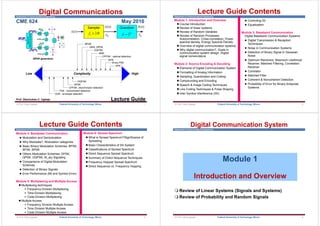
1. The document provides a lecture guide for a digital communications course covering topics like source encoding and decoding, baseband communication, bandpass communication, multiplexing, and spread spectrum.
2. The course is divided into 6 modules covering topics such as an introduction to signals and systems, random variables, probability, linear systems, Fourier transforms, and digital modulation schemes.
3. The guide outlines the contents of each module including reviews of prerequisite material and overviews of key concepts in digital communication systems.

![Department of Communications Engineering
Signals - 2
Mathematically, a signal is defined as a function of one
or more independent variables, e.g.,
x(t) = 10t
x(t) = 5t2
s(x,y) = 3x + 2xy + 10y2
Sometimes the functional dependence on the
independent variable is not precisely known, e.g.,
speech signal
Sometimes a signal is a combination of other signals
e.g., sum of sinusoid of different amplitudes,
frequency & phase
1
( ) ( )sin 2 ( ) ( )
n
i i i
i
s t A t F t t
© Prof. Okey Ugweje 9
Federal University of Technology, Minna
Department of Communications Engineering
Signals - 3
Mathematically, a signal is defined as a function of one or
more independent variables, e.g.,
x(t) = 10t
x(t) = 5t2
s(x,y) = 3x + 2xy + 10y2
Sometimes the functional dependence on the independent
variable is not precisely known, e.g., speech signal
Sometimes a signal is a combination of other signals
e.g., sum of sinusoid of different amplitudes, frequency & phase
Signals are the inputs outputs, and internal functions that
the systems process or produce, such as voltage,
current, pressure, displacements, intensity, etc.
1
( ) ( )sin 2 ( ) ( )
n
i i i
i
s t A t F t t
© Prof. Okey Ugweje 10
Federal University of Technology, Minna
Department of Communications Engineering
Signals - 4
The variable time may be continuous or discrete and the
value of the signal may be represented as
Continuous-valued x(t)
Discrete-valued x(nts)
Quantized xQ(t), and
Digital x[n]
These types of signals occur at different stages of the
process
Other variables (distance, angle, etc.) can also be the
independent variable, especially for 2-D signals like
images and video
© Prof. Okey Ugweje 11
Federal University of Technology, Minna
Department of Communications Engineering
Physical realizable signals must
Have time duration
Occupy finite frequency spectrum
Are continuous (as in analog signal)
Have finite peak value, and
Are real-valued
All real-world signals will have these properties
Sometimes we use mathematical signal models which violate
these conditions
e.g., Dirac delta function (or impulse function)
The most commonly used analog signals are the sinusoidal
signals (sine, cosine, etc.)
In communication systems, we are concerned with info
bearing signals that evolve as a function of the independent
variable, t
© Prof. Okey Ugweje 12
Federal University of Technology, Minna
Signals - 5](https://image.slidesharecdn.com/digital-communication-230215092539-7dc58e08/85/Digital-communication-pdf-3-320.jpg)

![Department of Communications Engineering
Broad Classification of Systems
We are
interested only
on the systems
that intersect the
dotted path.
Distributed
Parameters
SYSTEMS
Lumped Parameters
Stochastic Deterministic
Continuous Time Discrete Time
Nonlinear Linear
Nonlinear Linear
Time
Varying
Time
Invariant
Time
Varying
Time
Invariant
© Prof. Okey Ugweje 17
Federal University of Technology, Minna
Systems - 5 Department of Communications Engineering
Operation on Linear Systems
An operator, T, is a rule to transform one function to another
Additive
Homogeneous
Principle of Superposition
Superposition implies both additive & homogeneous rules
If a system fails either rule, the function is nonlinear
Addition or homogeneity is sufficient condition to test for
linearity
T x t y t
( ) ( )
T x t x t T x t T x t
1 2 1 2
( ) ( ) ( ) ( )
k p k p k p
T Kx t KT x t
( ) ( )
T Ax t Bx t AT x t BT x t
1 2 1 2
( ) ( ) ( ) ( )
k p k p k p
© Prof. Okey Ugweje 18
Federal University of Technology, Minna
Systems - 6
Department of Communications Engineering
Linear Time-Invariant (LTI) Systems
Linear systems are characterized by the ability to accept
input and produce output in response to the input
Most communication systems can be modeled as linear
systems with signals forming the input and output functions
h(t)
h[n]
H(ejw)
H(f)
H(z)
LTI
y(t)
y[n]
Y(ejw)
Y(f)
Y(z)
x(t)
x[n]
x(ejw)
X(f)
X(z)
Time Function
Pole-Zero Plot
Difference Equation
H - Function
Frequency Function
© Prof. Okey Ugweje 19
Federal University of Technology, Minna
Department of Communications Engineering
Why study signals and systems?
In signals and systems theory we study the definition
and description of signals, and the behavior of systems
under different conditions
Signals form the inputs, outputs and internal
functions of systems
In electrical & computer engineering, the understanding
of signals and the behavior of systems is of immense
importance
Communication engineers are concerned with systems
which transmit, receive, and process signals carrying
information
Hence before one can characterize a system, one must
be able to characterize the system
© Prof. Okey Ugweje 20
Federal University of Technology, Minna](https://image.slidesharecdn.com/digital-communication-230215092539-7dc58e08/85/Digital-communication-pdf-5-320.jpg)


![Department of Communications Engineering
Some Important or Common Signals & Functions
Sinusoidal Signal
Complex Exponential (harmonics)
Unit Step Function [denoted by u(t)]
Ramp Function [denoted by r(t)]
Rectangular Pulse Function [denoted by rect(t) or
(t)]
Triangular Pulse Function[denoted by (t)]
Sign (Signum) Function [denoted by sgn(t)]
Sinc Function [denoted by sinc(t)]
Impulse (Delta, Dirac) Function [denoted by (t)]
Signals and Spectra - 6
© Prof. Okey Ugweje 29
Federal University of Technology, Minna
Department of Communications Engineering
Operations on Signals
Amplitude Scaling
Amplitude Shifting
Time Shifting
Displaces a signal in time without changing its
shape
Signals and Spectra - 7
( ) ( )
"+"shifts the signal left by
"-" shifts the signal right by (delayed)
y t x t
© Prof. Okey Ugweje 30
Federal University of Technology, Minna
Department of Communications Engineering
Time Scaling
Slows down or speeds up time which results in signal
compression or stretching
The expression
Reflection or Folding
A scaling operation with = -1 x(t) = x(-t)
The mirror image of x(t) about the y-axis through t = 0
Operations in Combinations
x(t) delay (shift right) by x(t-)
compress by x(t-)
x(t) compress by x(t)
delay (shift right) by / x(t-)
Signals and Spectra - 8
( )
t
y t x
© Prof. Okey Ugweje 31
Federal University of Technology, Minna
Department of Communications Engineering
Some useful signal operations and models
Continuous/Discrete Convolution
Parseval’s’ theorem
Hilbert Transform
Concept of Bandwidth and Filtering
Some Important Properties of Signals
DC Value
Is the time average of a signal or the time average
over a finite interval [t1, t2]
Average Power
The ensemble average
RMS Value
Signals and Spectra - 9
© Prof. Okey Ugweje 32
Federal University of Technology, Minna](https://image.slidesharecdn.com/digital-communication-230215092539-7dc58e08/85/Digital-communication-pdf-8-320.jpg)


![Department of Communications Engineering
Digital Representation of Analog Signals
Most practical signal of interest are analog in nature
e.g., speech
biological signals
seismic signals
radar signals
sonar, and
various communication signals (audio, video, text, etc)
Conversion to digital form is necessary
Interface
(A/D)
Analog
Signal
Digital
Signal
© Prof. Okey Ugweje 73
Federal University of Technology, Minna
Department of Communications Engineering
Sampling
Digital Communication System
© Prof. Okey Ugweje 74
Federal University of Technology, Minna
Department of Communications Engineering
Digitization of Analog Signals
1. Sampling: obtain samples of x(t) at uniformly spaced
time intervals
2. Quantization: map each sample into an approximation
value of finite precision
Pulse Code Modulation: telephone speech
CD audio
3. Compression: to lower bit rate further, apply additional
compression method
Differential coding: cellular telephone speech
Subband coding: MP3 audio
Compression discussed in Chapter 12
© Prof. Okey Ugweje Federal University of Technology, Minna 75
Department of Communications Engineering
Transmitter Side Encoding
(Formatting Analog Information)
Structure of Digital Communication Transmitter
Analog-to-Digital (A/D) Conversion
Sampling Quantization
Digital
Modulation
Input
Signal
Transmitted
Signal
Transmitter
Sampler Quantizer
xa(t)
Analog signal
A/D Converter
Discrete-time
signal
Quantized
signal
x[n] xq
(n)
Quantized
Output Signal
Analog Input
Signal
© Prof. Okey Ugweje 76
Federal University of Technology, Minna](https://image.slidesharecdn.com/digital-communication-230215092539-7dc58e08/85/Digital-communication-pdf-19-320.jpg)


![Department of Communications Engineering
Quantization - 1
Sample values require infinite # of bits for perfect
representation since sampler output still continuous in
amplitude
each sample can take on any value, e.g. 4.752, 0.001, etc
the number of possible values is infinite
To transmit as a digital signal we must restrict the # of
possible values to finite bits
Sampler Quantizer
x(t)
Analog signal
A/D Converter
Discrete-time signal Quantized signal
x[n] xq
(n)
Analog
Input
signal
Quantized
output signal
© Prof. Okey Ugweje 89
Federal University of Technology, Minna
Department of Communications Engineering
Quantization - 2
Definition:
Quantization is the process of approximating
continuous-valued samples with a finite number of
bits
Quantizer
device that operates on a discrete-time signal to
produce finite # of amplitudes by approximating the
sampled values
maps each sampled value to one of pre-assigned
output levels
the process of “rounding off” a sample according to
some rule
© Prof. Okey Ugweje 90
Federal University of Technology, Minna
Department of Communications Engineering
e.g., suppose we must round to the nearest tenth,
then:
4.752 4.8
0.001 0
rounds off the sample values to the nearest
discrete value in a set of L quantum levels
quantized samples xq(n) are discrete in time (by
virtues of sampling) and discrete in amplitude (by
virtue of quantization)
Because we are approximating the analog sample
values by using finite # of levels, L, error is
introduced during quantization
Quantization - 3
© Prof. Okey Ugweje 91
Federal University of Technology, Minna
Department of Communications Engineering
Definition
number, size, location of its quantizing cell
boundaries, and step size of the quantization process
Quantization Resolution
# of bits, n, used to represent each sample
where L = number of levels
more bits results in better fidelity
However, the bit rate is higher and more bandwidth is required
Xq
(nT)
X[nT] Quantizer
random process
Quantizer Model and Definitions - 1
n L
log2
© Prof. Okey Ugweje 92
Federal University of Technology, Minna](https://image.slidesharecdn.com/digital-communication-230215092539-7dc58e08/85/Digital-communication-pdf-23-320.jpg)


![Department of Communications Engineering
Mathematical Description of Quantizer - 3
Signal-to-quantization noise ratio (SQNR) (or
simply SNR)
From above equation, average SNR can be written as
2
2
2
2 2
2
2
{ }
( )
( )
{ } { }
ˆ
( ) ( )
ˆ
avg
X
X
Signal Power
S
NoisePower
N
E x
E e t
x f x dx
E x E x
D x x f x dx
E x x
© Prof. Okey Ugweje 113
Federal University of Technology, Minna
Department of Communications Engineering
We have assumed
1. e(t) is uniformly distributed
2. {e(t)} is a stationary white noise process, i.e. e(j)
and e(k) are uncorrelated for j = k
3. e(t) is uncorrelated with the input signal x(t), and
4. signal sample xs(t) is zero mean and stationary
As a rule of thumb, each bit of quantization increases
the SNR by 6 dB provided that
a) xs(t) has a uniform distribution, and
b) the quantizer is a uniform quantizer
Mathematical Description of Quantizer - 4
© Prof. Okey Ugweje 114
Federal University of Technology, Minna
Department of Communications Engineering
If the input signal is a sequence, then
1
2
0
1
[ ]
N
S s
n
P x n
N
1
2
0
1
[ ]
N
N
n
P e n
N
1
2
0
1
2
0
[ ]
[ ]
N
s
S n
N
N
n
x n
P
SNR
P e n
Signal power
Noise power
Signal-to-noise ratio
Mathematical Description of Quantizer - 5
© Prof. Okey Ugweje 115
Federal University of Technology, Minna
Department of Communications Engineering
Given
q = step size, max quantization error is
where L = 2n is the # of quantization levels
The noise variance of the quantization error is given by
L/2 –1 positive levels
L/2 –1 negative levels
1 zero level
1
pp pp
V V
q
L L
SNR for Uniform Quantizer - 1
2 2 2 2
1 1
2 2 2
2 2 2
2
3 2
2
( ) ( ) ( ) ( )
1
3 12
q q q
q q q
q q
q
q
error p e de e de e de
q
e
q
Equation 13.12
L –1 level
L –2 intervals
This is the MSE
(noise variance)
© Prof. Okey Ugweje 116
Federal University of Technology, Minna](https://image.slidesharecdn.com/digital-communication-230215092539-7dc58e08/85/Digital-communication-pdf-29-320.jpg)


![Department of Communications Engineering
Non-uniform Quantization - 5
Error is the weighted sum of error powers in each
quantile
weighted by p(xn)qn
If the quantizer has uniform quantiles (i.e., UQ), then
If the Q does not operate in the saturation region, then
2
2
1
2 2
0
1
2
0
2
2
2 ( )
12
1
2
12 2
1
2 1
12 12
2 2
L
L
Lin n n n
n
n n
n n
q p x q
q q
q L
q
L
q q
q L
2 2
q Lin
125
Federal University of Technology, Minna
© Prof. Okey Ugweje
Department of Communications Engineering
##Uniform vs. Nonuniform Quantization
Let
Numerical integration will indicate that
However, NQ will yield a better result
The “best” possible quantizer has
NQ can give better performance for most signals than UQ
f x e
X
x
( )
1
2
2
2
. , . , . , .
x x x x
1 1494 2 0498 3 0498 4 1494
l q
D E x
01188 1
2
. , [ ]
S
N
dB
avg
F
H
I
K F
H
I
K
10
1
01188
9 25
10
log
.
.
S
N avg
dB
FH IK 12 0
.
126
Federal University of Technology, Minna
© Prof. Okey Ugweje
Department of Communications Engineering
Types of Noise in Quantizer
Overload Noise (Saturation Noise)
when input signal > Lmax resulting in clipping of signal
Granularity Noise (Quantization Noise)
when L are not finely spaced apart enough to accurately
approximate input signal
Truncation or Rounding error
This type of noise is signal dependent
Timing Jitter
Error caused by a shift in the sampler position
Easily isolated with stable clock reference and power
supply isolation
127
Federal University of Technology, Minna
© Prof. Okey Ugweje
Department of Communications Engineering
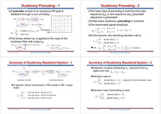
Reading Assignment:
Differential Quantization
Is used to reduce the dynamic range
Interpolation from previous value if samples are
correlated
Correlation can be increased by oversampling
Important/Practical Systems Using Quantization - 1
x
Differeence
Value
(k+2)T
(k+3)T
kT
Actual data
predited (linear interpolation)
Oversampling Predictor Differential
more samples/sec fewer samples/sec
128
Federal University of Technology, Minna
© Prof. Okey Ugweje](https://image.slidesharecdn.com/digital-communication-230215092539-7dc58e08/85/Digital-communication-pdf-32-320.jpg)
![Department of Communications Engineering
Differential PCM (DPCM)
Delta Modulation
Linear Predictive Coding
Adaptive Predictive Coding
Important/Practical Systems Using Quantization - 2
129
Federal University of Technology, Minna
© Prof. Okey Ugweje
20.Example 20
Quantization
21.Example 21
Uniform Qantrizer
Department of Communications Engineering
Example 22: (uniform quantization)
Sampler
f B
s 2
Quantizer
2n
L
x n
( )
xk
xk
( )
x n
x t
( )
n = # of binary bits used to
represent each sample
fs = sampling frequency or
sampling rate
= quantized
value of x(t)
2q
1
2 q
q k
x
ˆk
x
3q
2q
q
3q
3
2 q
5
2 q
7
2 q
1
2 q
3
2 q
5
2 q
7
2 q
111
110
101
100
011
010
001
000
ˆ ˆ[ ] [ ]
k q
x x n x n
Uniform Quantizer
130
Federal University of Technology, Minna
© Prof. Okey Ugweje
Department of Communications Engineering
Let the quantization level be {1,3,5,7}. Assume that
the input signal to a quantizer have the pdf shown
a) Compute the signal mean power
b) Compute the mean square error at the quantizer
output
c) Compute the output SNR
d) How would you change the distribution of the
quantization level in order to decrease the
distortion?
Example - Quantization
f x
x
else
x
( )
,
,
R
S
T
32 0 8
0
1
4
x t
( )
8
f x
( )
131
Federal University of Technology, Minna
© Prof. Okey Ugweje
Department of Communications Engineering
Federal University of Technology, Minna 132
Companding
Digital Communication System
© Prof. Okey Ugweje](https://image.slidesharecdn.com/digital-communication-230215092539-7dc58e08/85/Digital-communication-pdf-33-320.jpg)


![Department of Communications Engineering
Types of Companding - 2
In U.S., telephone lines uses = 255
Samples 4 kHz speech waveform at 8,000
sample/sec
Encodes each sample with 8 bits, L = 256 quantizer
levels
Hence data rate R = 64 kbit/sec
= 0 corresponds to uniform quantization
141
Federal University of Technology, Minna
© Prof. Okey Ugweje
Department of Communications Engineering
A-Law Companding (Europe, China, Russia, Asia,
Africa)
where
x and y represent the input and output voltages
A is a constant number determined by experiment, A = 87.6
You can find the companding gain by differentiating
the output
y x
y
A x
x
A
x
x
x A
y
A x
x
A
x
A
x
x
e
e
( )
sgn( ),
log
log
sgn( ),
max
max
max
max
max
max
FH IK
L
NM O
QP
R
S
|
|
|
T
|
|
|
1
0 1
1
1
1 1
G
d
dx
y x
x
( )
0
See eqn. 2.23
Types of Companding - 3
142
Federal University of Technology, Minna
© Prof. Okey Ugweje
Department of Communications Engineering
Federal University of Technology, Minna 143
Encoding
Digital Communication System
© Prof. Okey Ugweje
Department of Communications Engineering
Quantizer output is one of L possible signal levels
For binary transmission, each quantized sample is
mapped into an n-bit binary word
Encoding is the process of representing each of
the L outputs of the quantizer by an n-bit code
word
one-to-one mapping - no distortion introduced
xa(t)
Analog
signal
A/D Converter
Discrete-Time
signal
Quantized
signal
x[n] xq[n]
Sampler Quantizer
Line
Coder
an
Encoding - 1
144
Federal University of Technology, Minna
© Prof. Okey Ugweje](https://image.slidesharecdn.com/digital-communication-230215092539-7dc58e08/85/Digital-communication-pdf-36-320.jpg)


![Department of Communications Engineering
Pulse Code Modulation (PCM) - 3
153
Federal University of Technology, Minna
© Prof. Okey Ugweje
Department of Communications Engineering
Pulse Code Modulation (PCM) - 4
154
Federal University of Technology, Minna
© Prof. Okey Ugweje
Department of Communications Engineering
Advantages of PCM
Relatively inexpensive
Easily multiplexed
PCM waveforms from different sources can be
transmitted over a common digital channel (TDM)
Easily regenerated:
useful for long-distance communication e.g., telephone
Better noise performance than analog system
Modem is all digital, thus affording reliability, stability and is
readily adaptable to integrated circuits
Signals may be stored and time-scaled efficiently (e.g.,
satellite communication)
Efficient codes are readily available
Disadvantage
Requires wider bandwidth than analog signals
Pulse Code Modulation (PCM) - 5
155
Federal University of Technology, Minna
© Prof. Okey Ugweje
Department of Communications Engineering
Implementation of A/D Converters
Serial Input Output (SIO) circuit converts quantization
level to a sequence of bits n = log2 L
ADC SIO
( )
x f x
x n bits
Quantizer
Sampler Quantizer Coder
xa(t)
Analog signal
A/D Converter
Discrete-Time signal Quantized signal Digital signal
x[n] xq[n]
n
156
Federal University of Technology, Minna
© Prof. Okey Ugweje](https://image.slidesharecdn.com/digital-communication-230215092539-7dc58e08/85/Digital-communication-pdf-39-320.jpg)


![Department of Communications Engineering
Generation of Line Codes
Transmitter:
The FIR filter realizes the different pulse shapes
Baseband modulation with arbitrary pulse shapes can be detected by
correlation detector
matched filter detector (this is the most common detector)
ROM
Make
Impulse
h[n] = p[n]
0 -1
1 +1
binary
bits
an anp[n]
an [n]
s[n]
impulse train which
represents the data
pulse shape defined by impulse
response of FIR filter
N
5N
3N
2N
4N
0
1 1 1 1
0 0
N 5N
3N
2N 4N
0
1 1 1 1
0 0
241
Federal University of Technology, Minna
© Prof. Okey Ugweje
Department of Communications Engineering
Federal University of Technology, Minna 242
Pulse Shaping
Inter-symbol Interference
Digital Communication System
© Prof. Okey Ugweje
Department of Communications Engineering
Baseband Communication System
Baseband Communication System:
We have been considering the transmitter side
Transmitted signal is created by the line coder
according to
where an is the information sequence & g(t) is pulse shape
s t a g t nT
n b
n
( ) ( )
A/D
Converter
Line
Coder
Channel
Analog Input To Receiver
an s t
( )
Transmiter
A/D
Converter
Line
Coder
Channel
Input
an s t
( )
Transmiter
Decoder
A/D
Converter
Receiver
Output
243
Federal University of Technology, Minna
© Prof. Okey Ugweje
Department of Communications Engineering
Problems with Line Codes - 1
A) Line codes are not bandlimited
absolute bandwidth, B, is infinite
power outside the 1st null bandwidth is not negligible
i.e., power in the sidelobes can be quite high
This can cause Adjacent Channel Interference (ACI)
If transmission channel is bandlimited, then high freq
components will be cut off
High freq components correspond to sharp transition in
pulses
Hence, the pulse will spread out
If pulse spreads out into adjacent symbol period, then
inter-symbol interference (ISI) occurred
244
Federal University of Technology, Minna
© Prof. Okey Ugweje](https://image.slidesharecdn.com/digital-communication-230215092539-7dc58e08/85/Digital-communication-pdf-61-320.jpg)


![Department of Communications Engineering
At the output of the demodulator
where ai(t) is the signal component & noise n is zero mean
Gaussian
At the sampling instant t = T
For simplicity we will drop the index such that z = ai + n
0 0
1 1
( ) ( ) ( ), 0 for a binary 0
( )
( ) ( ) ( ), 0 for a binary 1
z t a t n t t T
z t
z t a t n t t T
0 0
1 1
( ) ( ) ( ), 0 for a binary 0
( )
( ) ( ) ( ), 0 for a binary 1
z T a T n T t T
z T
z T a T n T t T
Maximum Likelihood Detector (MLD) - 4
353
Federal University of Technology, Minna
© Prof. Okey Ugweje
Department of Communications Engineering
z(T) is known as decision variable or test statistics
and it is a random process corrupted by noise
Assume that pdf of z0(T) and z1(T) are Gaussian with
equal likelihood, and with 0 = a0, 1 = a1
a0
Region 0
Likelihood of s0
Region 1
Likelihood of s1
Decision
Line
P[z|s1 sent]
P[z|s0 sent]
Pe(s0)
a0
o
p z s z a
( | ) exp
0
0
0
0
2
1
2
1
2
F
HG I
KJ
L
NM O
QP
p z s z a
( | ) exp
1
1
1
1
2
1
2
1
2
F
HG I
KJ
L
NM O
QP
Minimum error criterion
0
0 1
2
0
a a
Maximum Likelihood Detector (MLD) - 5
354
Federal University of Technology, Minna
© Prof. Okey Ugweje
Department of Communications Engineering
This is an averaging operation
It makes sense because the logical point is halfway
between the two voltage levels representing each
symbol
Questions:
How do we implement this averaging operation?
How do we choose the threshold, 0?
Hypothesis:
H0: r(t) = s0(t) + n(t) “0” sent
H1: r(t) = s1(t) + n(t) “1” sent
Maximum Likelihood Detector (MLD) - 6
355
Federal University of Technology, Minna
© Prof. Okey Ugweje
Department of Communications Engineering
Definitions of Probabilities:
P[s0], P[s1] a priori probabilities
These probabilities are known before transmission
P[z]
probability of the received sample
p(z|s0), p(z|s1)
conditional pdf of received signal z, conditioned on the class si
P[s0|z], P[s1|z] a posteriori probabilities
After examining the sample, we make a refinement of our previous
knowledge
P[s1|s0], P[s0|s1]
wrong decision (error)
P[s1|s1], P[s0|s0] correct decision
Maximum Likelihood Detector (MLD) - 7
356
Federal University of Technology, Minna
© Prof. Okey Ugweje](https://image.slidesharecdn.com/digital-communication-230215092539-7dc58e08/85/Digital-communication-pdf-89-320.jpg)
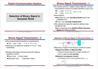
![Department of Communications Engineering
Decision Rule:
Acquiring information at the receiver about the transmitted
signal involves making decisions
We must decide which of the set of hypothesis best
describes the received signal
This involves uncertain (error in judgment)
If the signals we are trying to detect do not overlap, we
can make a decision without error
On the contrary, we need some rules to help classify the
received signal once they fall in the overlap region
A set of rules known as decision rules allow us to decide
( )
ˆi
z t
0
z T
( )
1
H
0
H
Maximum Likelihood Detector (MLD) - 8
357
Federal University of Technology, Minna
© Prof. Okey Ugweje
Department of Communications Engineering
1. Bayes’ decision criterion:
It formulates the problem of making a decision
under conditions of uncertainty by selecting the
hypothesis with the greatest a posteriori probability
This scheme assumes that some errors are more
costly than others
Hence, it assigns cost (weighting factors) that
reflect the risk involved
This is the most widely applied decision rule in
communications
Types of Decision Rules - 1
358
Federal University of Technology, Minna
© Prof. Okey Ugweje
Department of Communications Engineering
2. Maximum a posteriori (MAP) criterion:
Decide that the received signal belongs to the class
with the maximum a posteriori probabilities, i.e.,
maximize P(si|z)
It equivalently examines the pdf conditioned on
each signal class (p(z|s0), p(z|s1)) and choose the
maximum
For the received signal za, the likelihood that za
belongs to s1 or s2 corresponds to the circled point
on the pdf
The decision criterion is based on the likelihood of
P[z|si], i = 0,
Types of Decision Rules - 2
359
Federal University of Technology, Minna
© Prof. Okey Ugweje
Department of Communications Engineering
3. Newman-Pearson (N-P) criterion
Makes no assumption on the a priori source
statistics (requires only a posteriori probabilities)
Widely used in pulse detection in Gaussian noise as
in Radar applications where the source probabilities
(presence or absence of a target) is unknown
fix probability of false alarm
minimize probability of error
maximize probability of correct decision
Types of Decision Rules - 3
360
Federal University of Technology, Minna
© Prof. Okey Ugweje](https://image.slidesharecdn.com/digital-communication-230215092539-7dc58e08/85/Digital-communication-pdf-90-320.jpg)
![Department of Communications Engineering
4. Min-max criterion
Also in this criterion, the a priori probability is not
known
Since P(H1) is unknown, the rule maximizes the risk
with respect to P(H1) and minimizes the risk with
respect to P(H0)
Types of Decision Rules - 4
361
Federal University of Technology, Minna
© Prof. Okey Ugweje
Department of Communications Engineering
Bayes’ Decision Criterion - 1
Recall that the Bayes equation is given by
where
Recall from probability theory that
In communications, we can interpret the Bayes’
equation as a description of an experiment involving
a received sample, and
a statistical knowledge of the signal classes to
which the received sample may belong
1
[ ] [ | ] [ ]
M
i i
i
P z P z s P s
[ | ] [ ]
[ | ] , 0,2, , 1
[ ]
i i
i
P z s P s
P s z i M
P z
[ | ] [ ] ( | ) [ ]
i i i
P s z P z p z s P s
362
Federal University of Technology, Minna
© Prof. Okey Ugweje
Department of Communications Engineering
That is,
si denote the ith transmitted signal class from a set
of M classes
zj denotes the jth sample of the received signal
Hence, we can write the Bayes equation in terms of
the pdf
where
( | ) [ ]
[ | ] , 0,2, , 1
( )
i i
i
p z s P s
P s z i M
p z
1
( ) ( | ) [ ]
M
i i
i
p z p z s P s
Bayes’ Decision Criterion - 2
363
Federal University of Technology, Minna
© Prof. Okey Ugweje
Department of Communications Engineering
By examining a particular received sample zj, it is
possible to find likelihood that zj belongs to class si
This means that after the experiment, we will refine our
knowledge by computing the a posteriori probability
Note that the terms a priori and a posteriori imply
“cause to effect” and “effect to cause,” respectively
Assume that
Pdf of z0(T) and z1(T) are Gaussian with equal
likelihood, having mean values of a0 and a1 respectively
a0 and a1 are mutually independent
Noise n0 is independent zero mean AWGN with PSD No
Bayes’ Decision Criterion - 3
364
Federal University of Technology, Minna
© Prof. Okey Ugweje](https://image.slidesharecdn.com/digital-communication-230215092539-7dc58e08/85/Digital-communication-pdf-91-320.jpg)
![Department of Communications Engineering
In this case, for binary signal
The last equation corresponds to making a decision
based on the comparison of received signal to some
threshold level
1 0
[ | ] [ | ] decision rule
P s z P s z
0 0
1 1 ( | ) [ ]
( | ) [ ]
( ) ( )
p z s P s
p z s P s
p z p z
1 1 0 0
( | ) [ ] ( | ) [ ]
p z s P s p z s P s
0
1
0 1
[ ]
( | )
( ) likelihood ratio test (LRT)
( | ) [ ]
P s
p z s
L z
p z s P s
Bayes’ Decision Criterion - 4
365
Federal University of Technology, Minna
© Prof. Okey Ugweje
Department of Communications Engineering
The right-hand side (RHS) is called the likelihood ratio
When the two signals, s0(t) and s1(t), are equally likely,
i.e., P[s0] = P[s1] = 0.5, then the decision rule becomes
In terms of the Bayes criterion, it implies that the cost of
both types of error is the same
This type of decision rule is called the maximum a
posteriori (MAP) criterion (or minimum error
criterion)
0
1
0 1
[ ]
( | )
( ) likelihood ratio test (LRT)
( | ) [ ]
P s
p z s
L z
p z s P s
1
0
( | )
( ) 1 max likelihood ratio test
( | )
p z s
L z
p z s
Bayes’ Decision Criterion - 5
366
Federal University of Technology, Minna
© Prof. Okey Ugweje
Department of Communications Engineering
Substituting the pdfs
2
0
0 0
0 0
1 1
: ( | ) exp
2 2
z a
H p z s
2
1
1 1
1 1
1 1
: ( | ) exp
2 2
z a
H p z s
2
1
2
1
1 1
2
0
0
2
0
0
1
1
( )
exp
2
( | ) 2
( ) 1 1
1
1
( | )
( )
exp
2
2
z a
p z s
L z
p z s
z a
2 2
0 1
2 2
1 0 1 0
2 2
0 0
( ) ( )
exp 1
2
z a a a a
Bayes’ Decision Criterion - 6
367
Federal University of Technology, Minna
© Prof. Okey Ugweje
Department of Communications Engineering
Taking the log of both sides will give
Hence
where z is minimum error criterion and 0 is optimum threshold
2 2
1 0 1 0
2 2
0 0
( ) ( )
ln{ ( )} 0
2
z a a a a
L z
2 2
1 0 1 0 1 0 1 0
2 2 2
0 0 0
( ) ( )( )
2 2
z a a a a a a a a
2
0 1 0 1 0
2
0 1 0
( )( )
2 ( )
a a a a
z
a a
1 0
0
( )
2
a a
z
Bayes’ Decision Criterion - 7
368
Federal University of Technology, Minna
© Prof. Okey Ugweje](https://image.slidesharecdn.com/digital-communication-230215092539-7dc58e08/85/Digital-communication-pdf-92-320.jpg)
![Department of Communications Engineering
For antipodal signal, s1(t) = - s0(t) a1 = - a0
This means that if received signal was positive, s1(t)
was sent, else s0(t) is sent
0
z
Bayes’ Decision Criterion - 8
369
Federal University of Technology, Minna
© Prof. Okey Ugweje
Department of Communications Engineering
Probability of Error - 1
Error will occur if
s1 is sent s0 is received
P[H0|s1] = P[e|s1]
s0 is sent s1 is received
P[H1|s0] = P[e|s0]
The total probability of error is the sum of the errors
0
1 1
[ | ] ( | )
P e s p z s dz
0 0
0
[ | ] ( | )
P e s p z s dz
2
1 1 0 0
1
0 1 1 1 0 0
( , ) [ | ] [ ] [ | ] [ ]
[ | ] [ ] [ | ] [ ]
B i
i
P P e s P e s P s P e s P s
P H s P s P H s P s
o
ao a1
0 1
o
ao a1
0 1
See pp. 121~122 & section
B.2
370
Federal University of Technology, Minna
© Prof. Okey Ugweje
Department of Communications Engineering
If signals are equally probable
Hence, PB, is probability that an incorrect hypothesis is
made
Think of PB as the area under the tail of either of the
conditional distributions, p(z|s1) or p(z|s2), i.e.,
0 1 1 1 0 0
1
0 1 1 0
2
[ | ] [ ] [ | ] [ ]
[ | ] [ | ]
B
P P H s P s P H s P s
P H s P H s
1
1 0
0 1 1 0
2
[ | ]
[ | ] [ | ]
B
by symmetry
P P H s
P H s P H s
1 0 0
0 0
2
0
0
0 0
( | ) ( | )
1 1
exp
2 2
B
P p H s dz p z s dz
z a
dz
Probability of Error - 2
371
Federal University of Technology, Minna
© Prof. Okey Ugweje
Department of Communications Engineering
This equation cannot be evaluated in closed form
This is the famous Q-function or complementary error
function
Hence,
1 0
0
2
B
a a
P Q
1 0
2
0
0
0 0
0
0
0
2
( )/ 2
1
1 1
exp
2 2
( )
,
1
exp *
2 2
B
a a
z a
P dz
z a
u du dz
u du A
Probability of Error - 3
372
Federal University of Technology, Minna
© Prof. Okey Ugweje](https://image.slidesharecdn.com/digital-communication-230215092539-7dc58e08/85/Digital-communication-pdf-93-320.jpg)
![Department of Communications Engineering
Pe is minimized by choosing h(t) or H(f) such that optimum
threshold 0 is minimized
That is
A note on the Q(x) - complementary (co) error function
Equivalent Definitions
For large arguments (x large), Q function
2
2
0 1 0 1
0 0
( ) ( ) [ ( ) ( )]
2 4
a t a t a T a T
or
2
1
( ) exp
2 2
x
Q x
x
1
( ) e
2 2
x
Q x rfc
e 2 2
rfc Q
x x
Probability of Error - 4
373
Federal University of Technology, Minna
© Prof. Okey Ugweje
Department of Communications Engineering
Federal University of Technology, Minna 374
Correlator
© Prof. Okey Ugweje
Department of Communications Engineering
Correlator-Type Receiver - 1
The correlator cross-correlates r(t), with the 2
possible transmitted symbols s0(t) and s1(t)
Output for either z0 or z1 is given by
This cross-correlation process basically computes the
projection of r(t) into 2 basis functions s0(t) and s1(t)
The outputs z0 and z1 are then feed to the Threshold Detector
x
Threshold
Detector
r t
( ) s t
0
( )
t T
z T
0
( )
( )
s t
i
x
z T
1
( )
s t
1
( )
()
z dt
T
0
()
z dt
T
0
z t
0
( )
z t
1
( )
0 0
0
( ) ( ) ( )
T
z T r t s t dt
1 1
0
( ) ( ) ( )
T
z T r t s t dt
375
Federal University of Technology, Minna
© Prof. Okey Ugweje
Department of Communications Engineering
Correlator-Type Receiver - 2
The detector compares z1 and z0 and decides that
1 was transmitted if z1 > z0
0 was transmitted if z1 < z0
So when s1(t) is transmitted,
PB = P[z0 > z1] = P[n0 > E + n1] = P[n0 -n1> E]
Let x = n0 - n1
2
2 2 2
0 1 0 1 0 1
2 2
0 0
0
2
2 ( ) 2
4 2
n
E x zeromean
E x E n n E n E n E n n
N N
E n t
0, orthogonal
Noise Variance
376
Federal University of Technology, Minna
© Prof. Okey Ugweje](https://image.slidesharecdn.com/digital-communication-230215092539-7dc58e08/85/Digital-communication-pdf-94-320.jpg)


![Department of Communications Engineering
From (b):
But
At sampling instant t = T, we have
This is the same result obtained in (a)
Hence
z T z T
( ) '( )
h t s T t h t s T t s T t
( ) ( ) ( ) [ ( )] ( )
z
z t r s T t d
t
'( ) ( ) ( )
0
z t r t h t r h t d r h t d
t
'( ) ( ) ( ) ( ) ( ) ( ) ( )
z
z
0
' '
0
0
( ) ( ) ( ) ( )
( ) ( )
T
t T
T
T
z t z r s T T d
r s d
Correlator vs. Matched Filter - 2
397
Federal University of Technology, Minna
© Prof. Okey Ugweje
Department of Communications Engineering
Examples
Example Signal to Noise Ratio
Example Correlator Output
Example Matched Filter
398
Federal University of Technology, Minna
© Prof. Okey Ugweje
Department of Communications Engineering
#Generalized One Dimensional Signals - 1
One Dimensional Signal Constellation
-A +A
so s1
M=2
0
-A +A
s1 s2
M=4
0
-3A
so
+3A
s3
-5A -3A
s1 s2
M=8
0
-7A
so
-A
s3
+3A +5A
s5 s6
+A
s4
+7A
s7
E A A A
avg
2 2
2
2
E A A A A A
avg
9 9
4
5
2 2 2 2
2
E A A A A A A A A A
avg
49 25 9 9 25 49
8
21
2 2 2 2 2 2 2 2
2
399
Federal University of Technology, Minna
© Prof. Okey Ugweje
Department of Communications Engineering
Binary Baseband Orthogonal Signals
Binary Antipodal Signals
Binary Orthogonal Signals
2-Dimensional Signal Constellation
An example:
+A
+A
s1
s0
1
E A A A
avg
2 2
2
2
2
-A +A
so
s1
0
1
E A A A
avg
2 2
2
2
1( )
t
1 2 0
( ) ( )
t t dt
o
T
z
2
( )
t
1
T
T
1
T
1
T
T t
2
T
2
T
#Generalized One Dimensional Signals - 2
400
Federal University of Technology, Minna
© Prof. Okey Ugweje](https://image.slidesharecdn.com/digital-communication-230215092539-7dc58e08/85/Digital-communication-pdf-100-320.jpg)


![Department of Communications Engineering
3. Complex Envelope (CE) Representation
Any bandpass signal can also be represented as
where g(t) = complex envelope - complex-valued signal
S(t) is convenient in many instances for analysis. Why?
Compact
Easy to manipulate without recourse to trig. identities
Relationship: Complex Envelope and M&P Forms
To transform from CE to M&P:
R(t) = |g(t)|, (t) = g(t)
To transform from M&P to CE:
g(t) = R(t)ej(t)
( ) Re ( )exp( )
c
s t g t j t
‡ Representation of Bandpass Signals
© Prof. Okey Ugweje 425
Federal University of Technology, Minna
Department of Communications Engineering
Relationship: CE and I & Q Forms
To transform from CE to I&Q:
x(t) = Re[g(t)], y(t) = Im[g(t)]
s(t) = Re[g(t)ejt] = Re[(x(t)+jy(t)).(cosct+jsinct)]
= x(t)cosct - y(t)sinct
Relationship between Spectral Representations
Assume that
Fourier Transform (Deterministic Signals):
( ) Re ( )
j t
c
s t g t e
S f G f fc G f fc
( ) ( ) ( )
1
2
‡ Representation of Bandpass Signals
© Prof. Okey Ugweje 426
Federal University of Technology, Minna
Department of Communications Engineering
Power Spectral Density (Random Signals):
Relationship: Power and Envelope of Bandpass
Power of bandpass signal is one half of power in
complex envelope:
G f G f f G f f
s g c g c
( ) ( ) ( )
1
4
2
(0)
1 1 1
( ) (0)
2 2 2
s s
g g
G R
g t R G
‡ Representation of Bandpass Signals
© Prof. Okey Ugweje 427
Federal University of Technology, Minna
Department of Communications Engineering
Bandpass Modulation & Demodulation - 1
Format Multiplex
Channel
Encoder
Source
Encoder
Spread
Format Demultiplex
Channel
Decoder
Source
Decoder
Despread
Performance
Measure Bits or
Symbol
To other
destinations
From other
sources
Digital
input
Digital
output
Source
bits
Source
bits
Channel
bits
Carrier and symbol
synchronization
Channel
bits
mi
l q
mi
l q
Pe
Multiple
Access
Waveforms
Multiple
Access
Modulate
Demodulate
&
Detect
428
Federal University of Technology, Minna
© Prof. Okey Ugweje](https://image.slidesharecdn.com/digital-communication-230215092539-7dc58e08/85/Digital-communication-pdf-107-320.jpg)


![Department of Communications Engineering
Quadrature Amplitude Modulation - 1
The most commonly used combination of amplitude
and phase signaling is the Quadrature Amplitude
Modulation (QAM)
Some books regard it as an extension of the QPSK
since it consist of two independent amplitude-
modulated carrier in quadrature. i.e.,
where ai and bi are amplitude levels obtained by
mapping k-bit sequence into amplitudes, or
where g(t) is the signal pulse shaping function
2
( ) [ cos sin ]
i i o i o
E
s t a t b t
T
( ) ( )[ cos sin ]
i i o i o
s t g t a t b t
553
Federal University of Technology, Minna
© Prof. Okey Ugweje
Department of Communications Engineering
Quadrature Amplitude Modulation - 2
It is sometimes regarded as M-ary APK with
constraints put on the amplitude and phase
where
In this case, both the amplitude and phase can be
varied
Any combination of M1-level amplitude and M2-level
phase can be used in the construction of QAM
1 2
2
( ) cos[ ], 1,2, , , 1,2, ,
i i o j
E
s t V t i M j M
T
1 2 2 1 2
2 , 2 , log ,
m n
M M m n M M
b
s
R
R
m n
554
Federal University of Technology, Minna
© Prof. Okey Ugweje
Department of Communications Engineering
Any combination of M1-level amplitude and M2-level
phase can be used in the construction of QAM
QAM waveform can be represented as a linear
combination of 2 orthogonal signals 1(t) and 2(t)
where
In vector notation:
1 2
( ) ( ) ( )
i i i
s t A t B t
1 2
2 2
( ) cos[ ], ( ) sin[ ]
o o
T T
s s
t t t t
1 2
, , ,
i i i i i i i
s s s A E B E a b
Quadrature Amplitude Modulation - 3
555
Federal University of Technology, Minna
© Prof. Okey Ugweje
Department of Communications Engineering
Using the vector representation, we can realize an L-
by-L matrix representing the coordinates of (ai, bi)
where
( 1, 1) ( 3, 1) ( 1, 1)
( 1, 3) ( 3, 3) ( 1, 3)
{ , }
( 1, 1) ( 3, 1) ( 1, 1)
L L L L L L
L L L L L L
a b
i i
L L L L L L
L M
Quadrature Amplitude Modulation - 4
556
Federal University of Technology, Minna
© Prof. Okey Ugweje](https://image.slidesharecdn.com/digital-communication-230215092539-7dc58e08/85/Digital-communication-pdf-139-320.jpg)