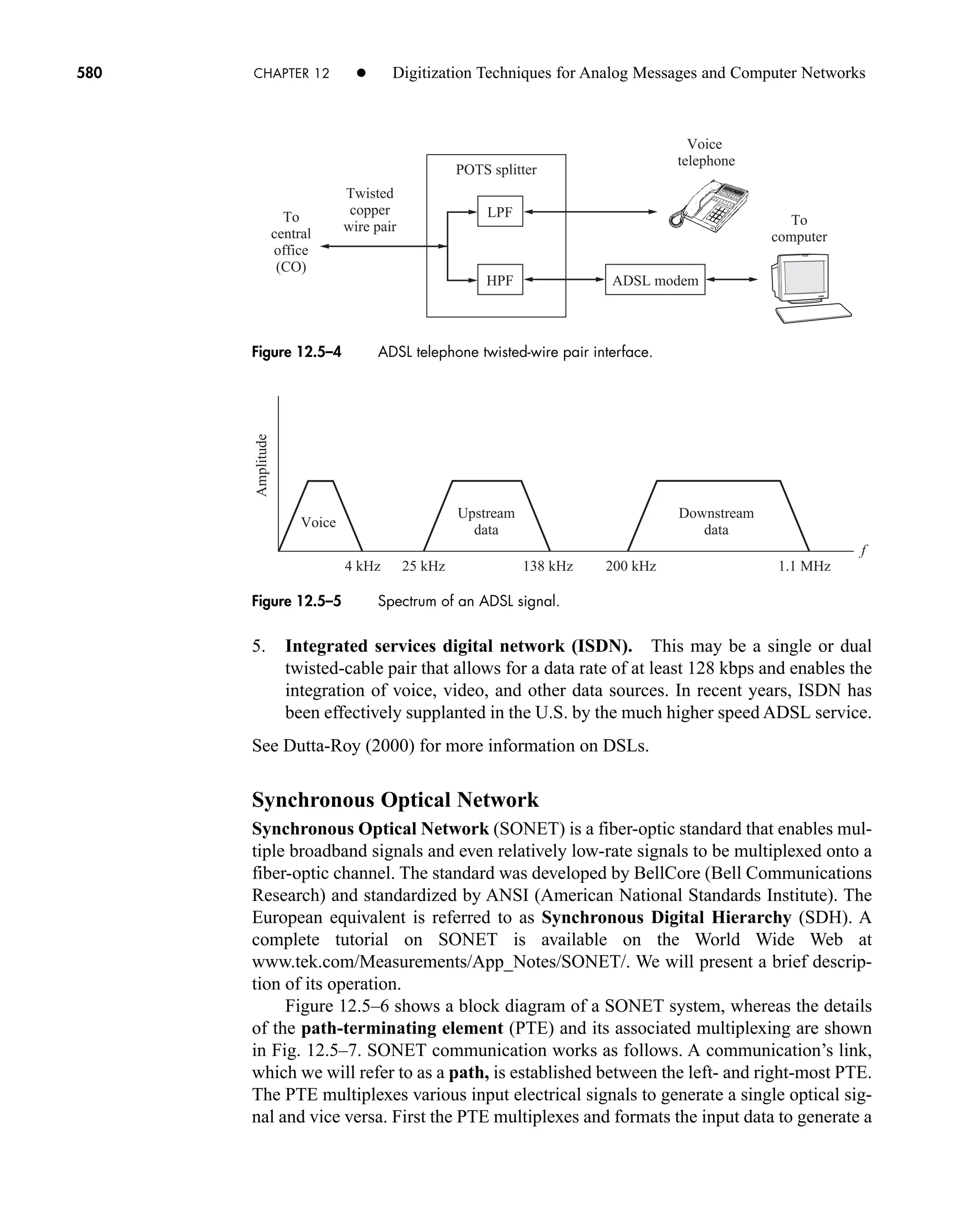
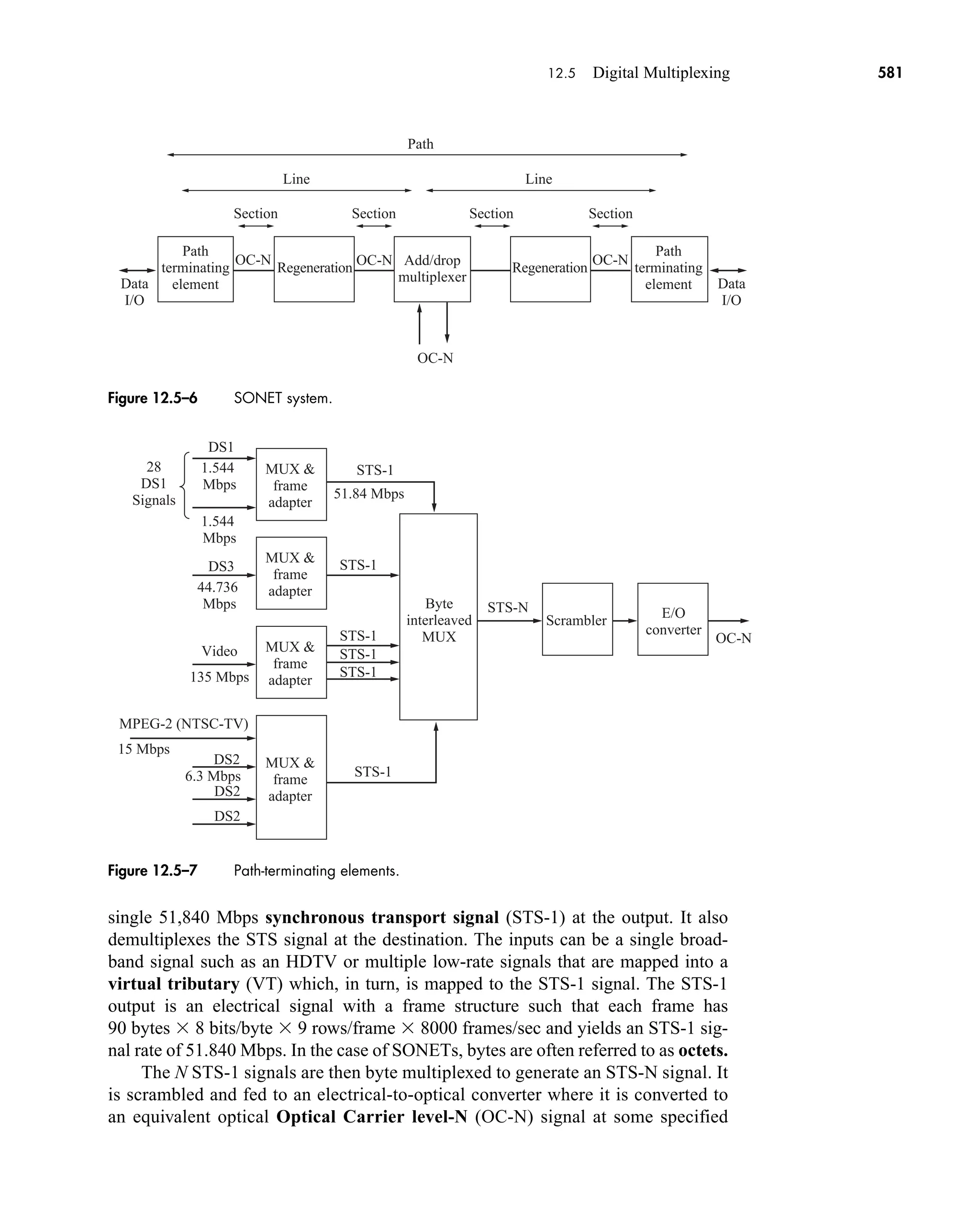
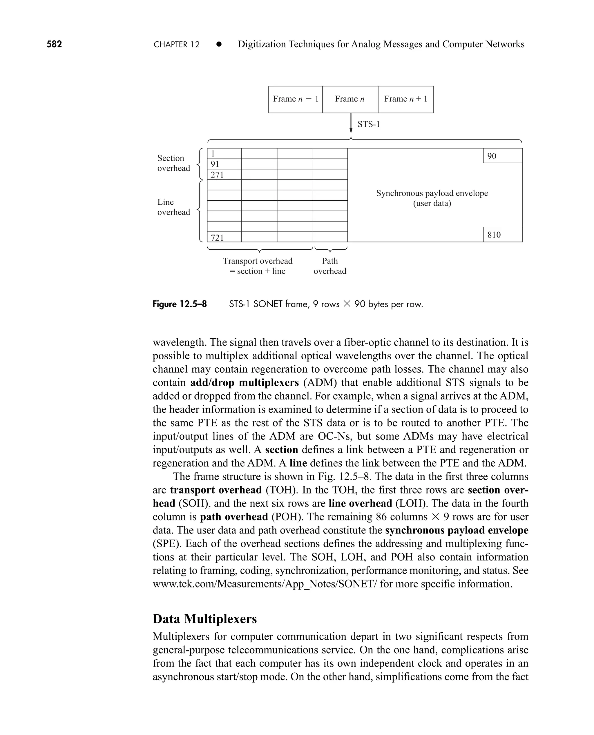
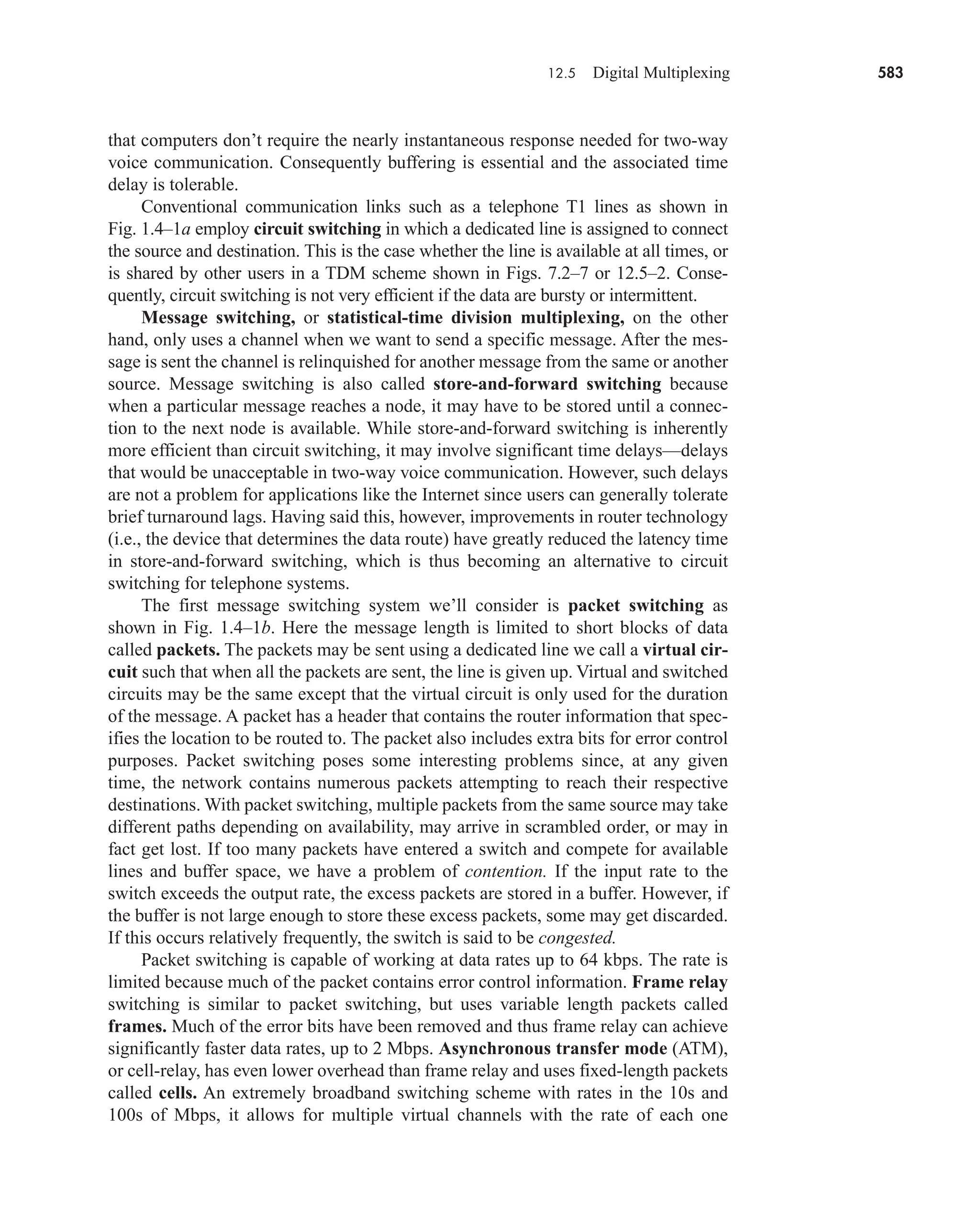
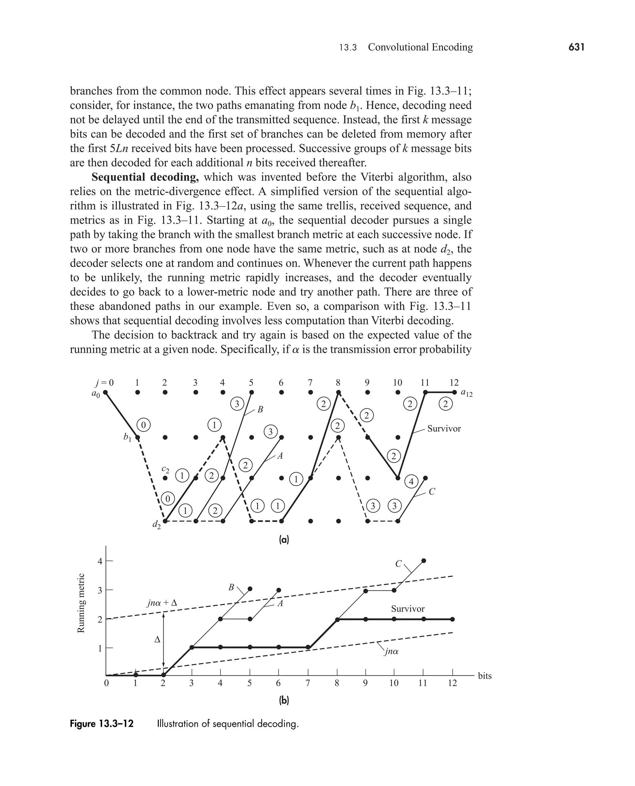
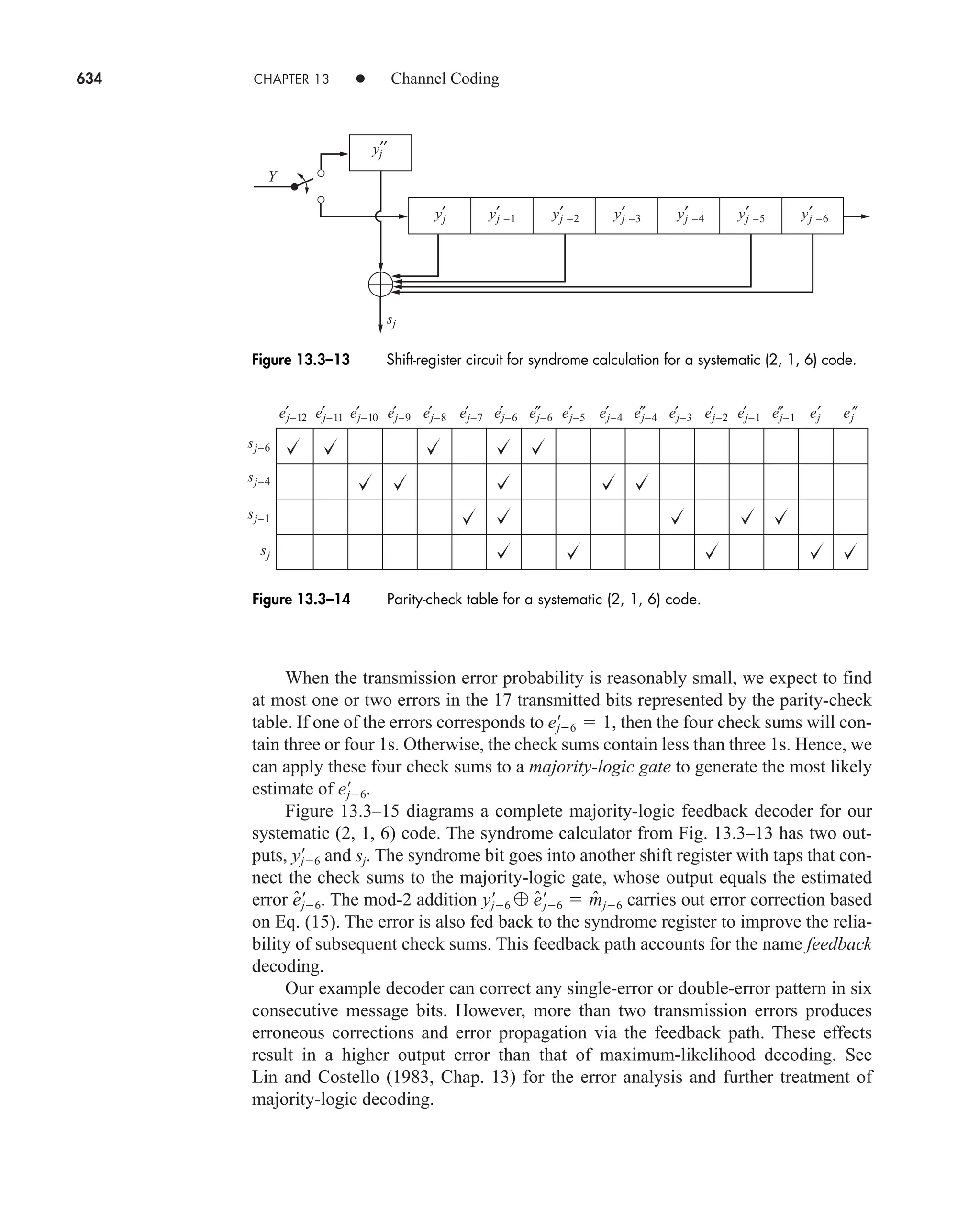
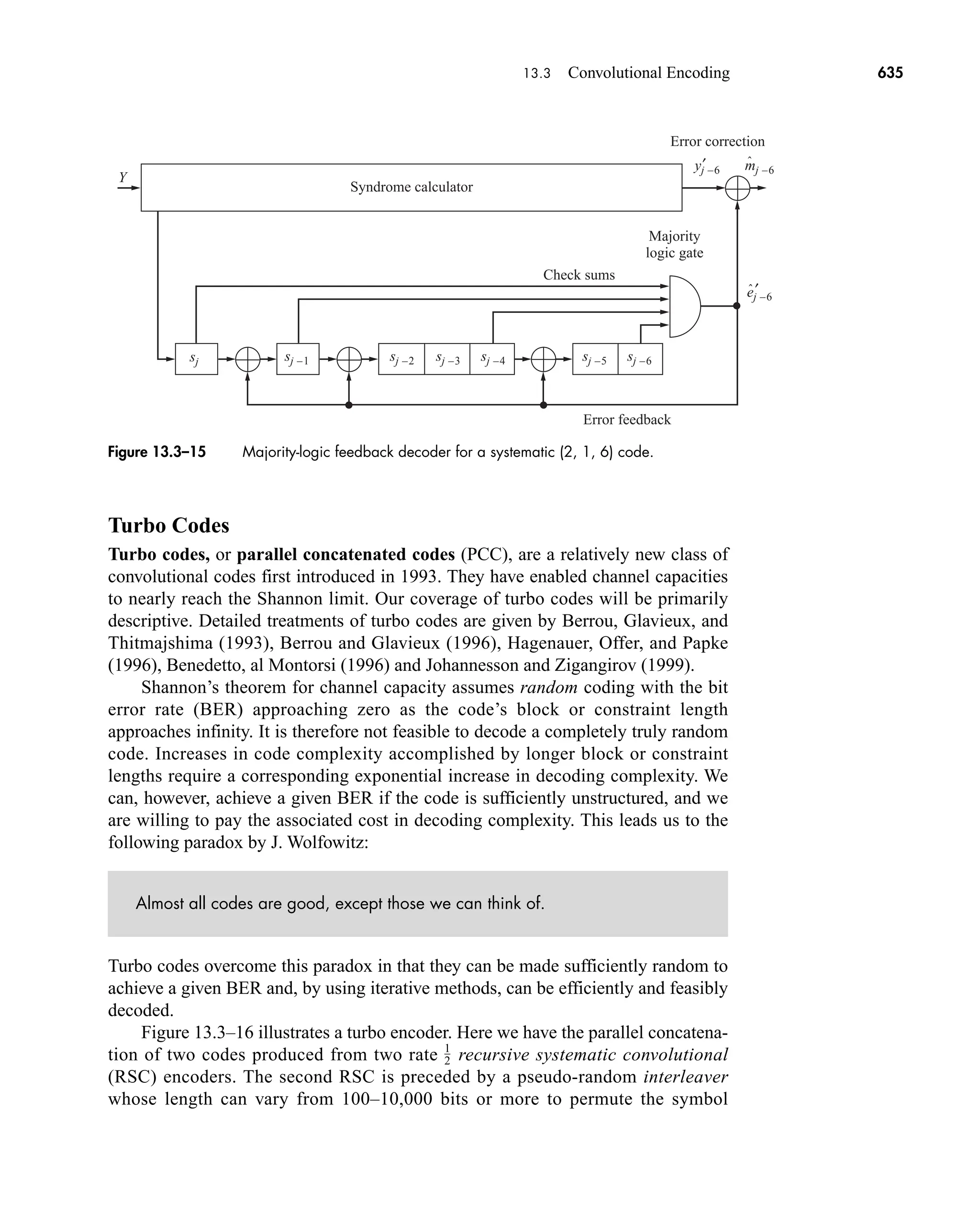
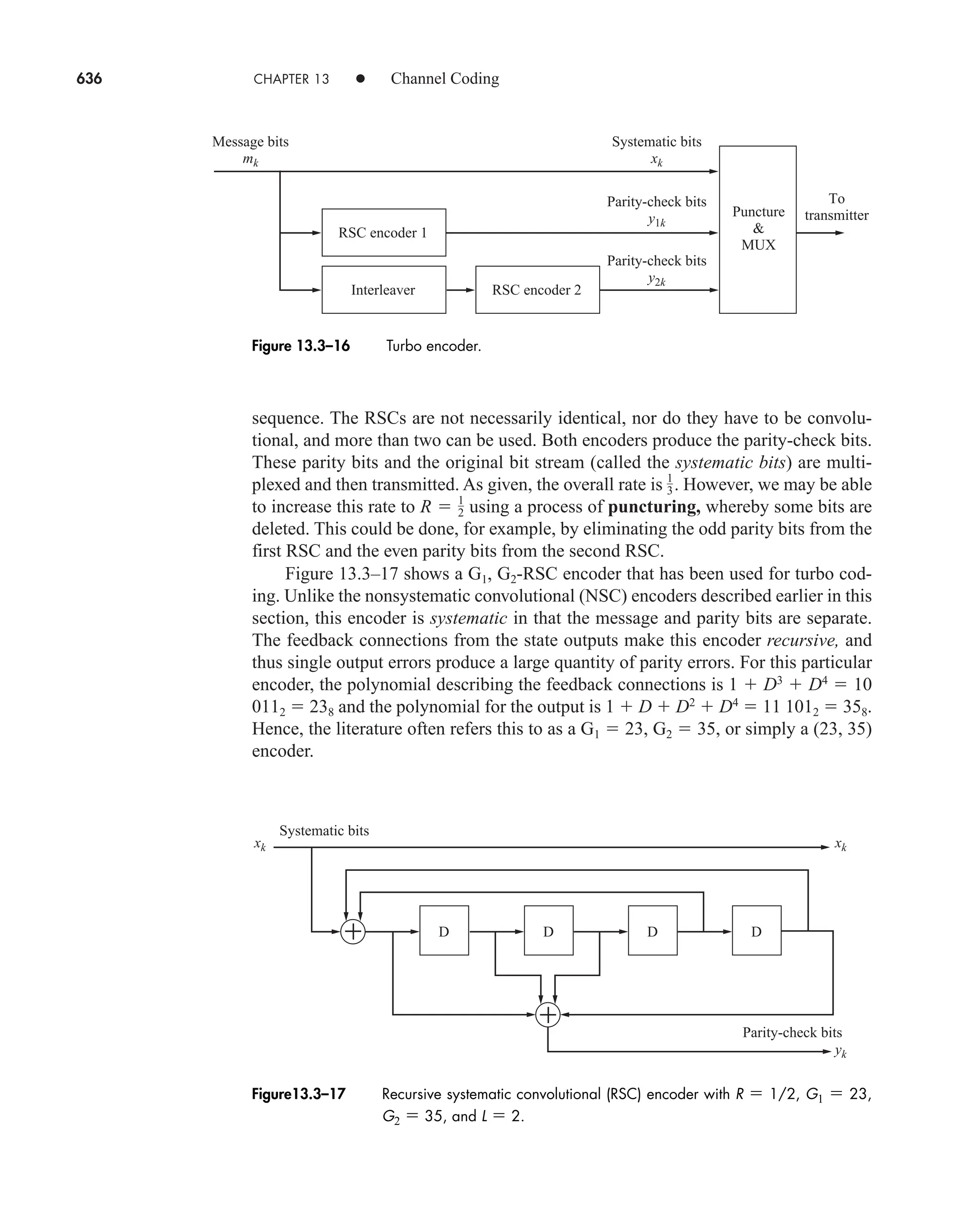
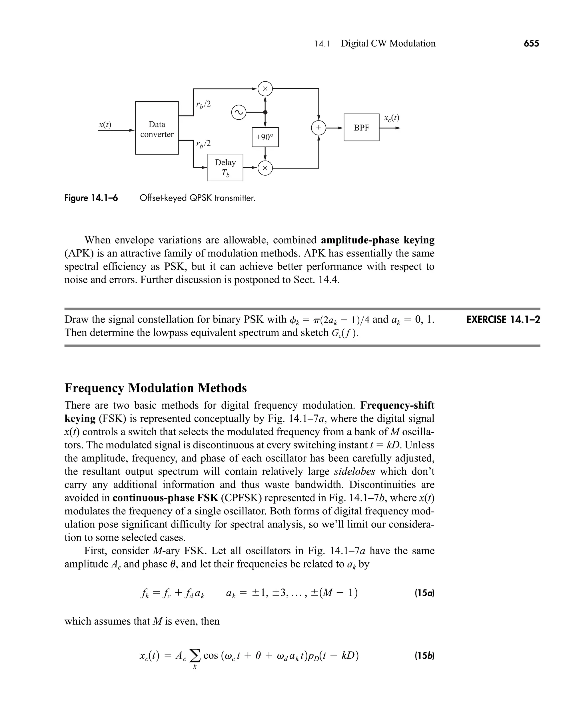
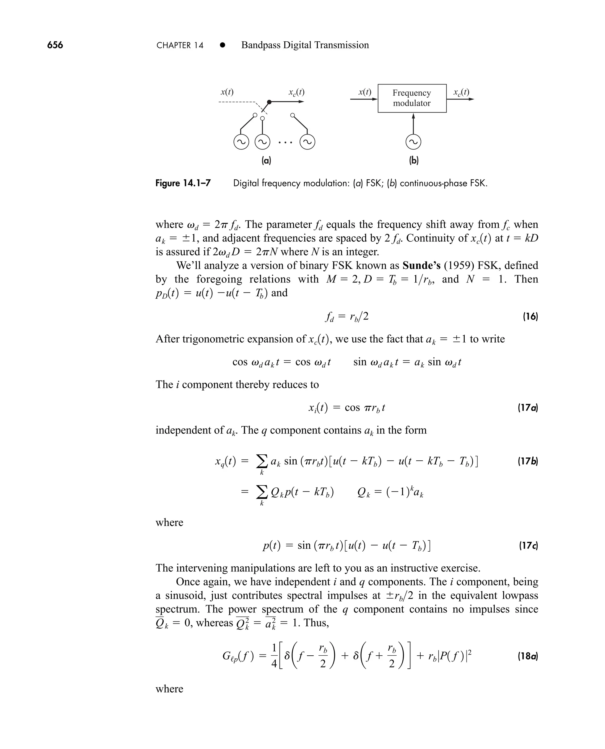
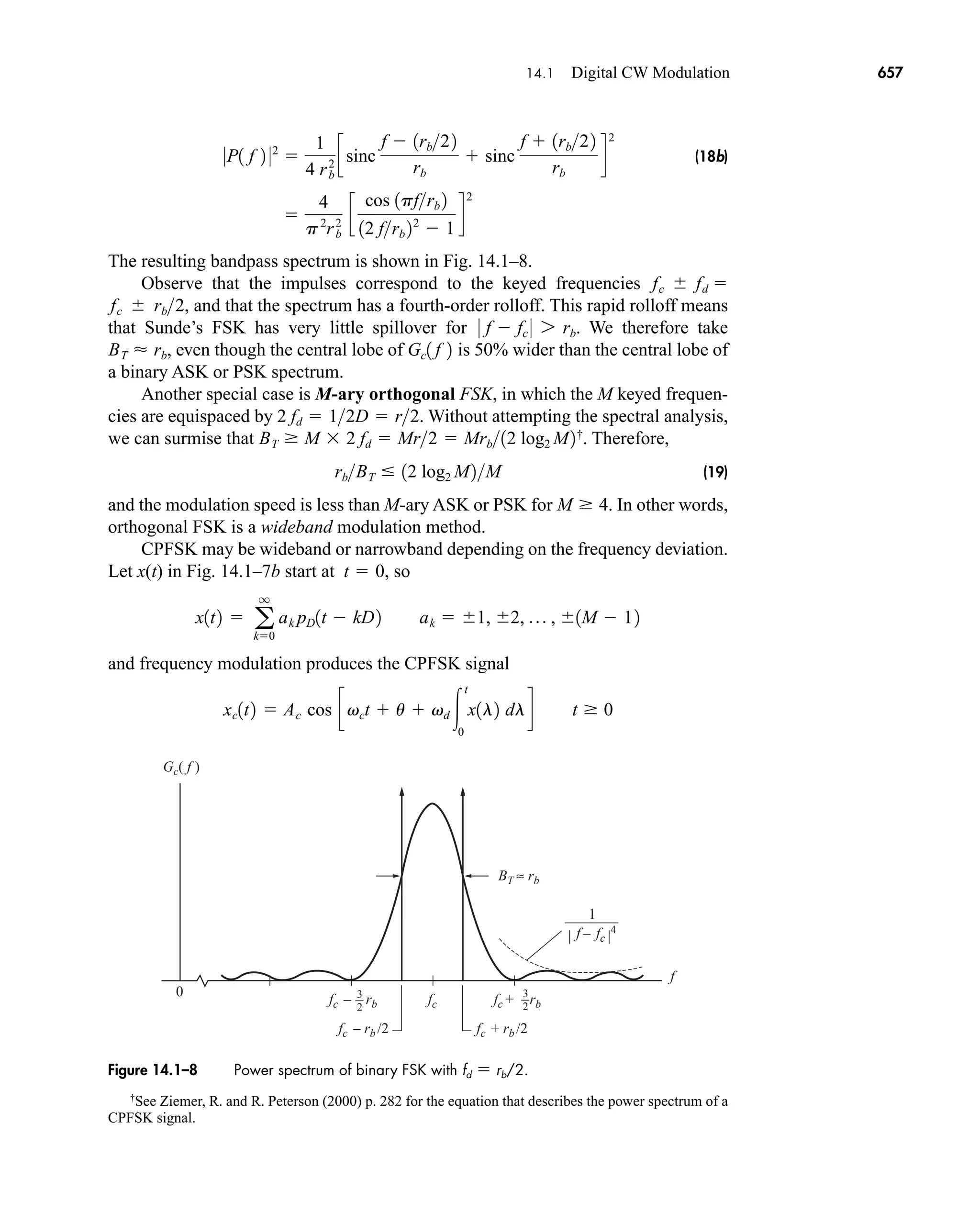
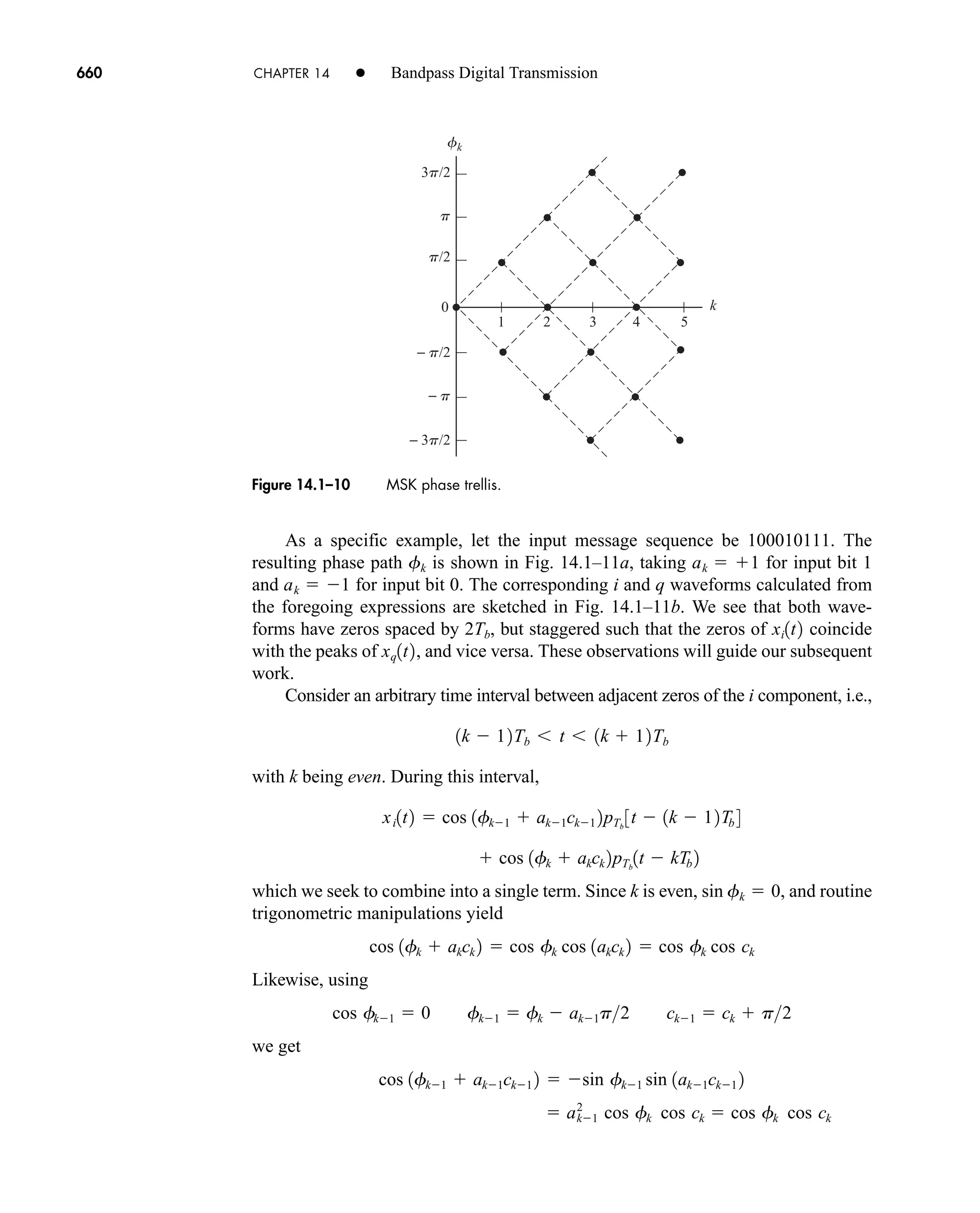
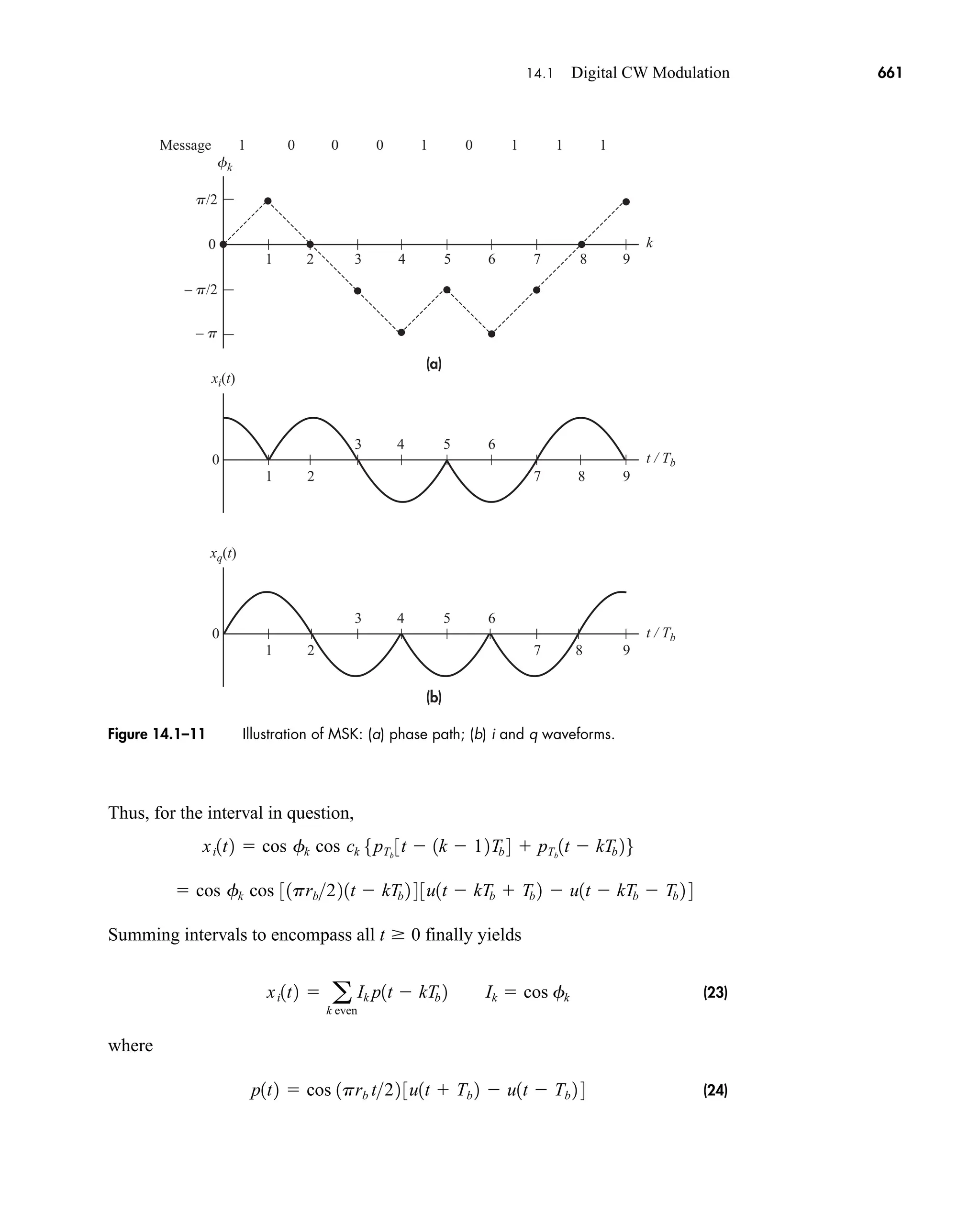
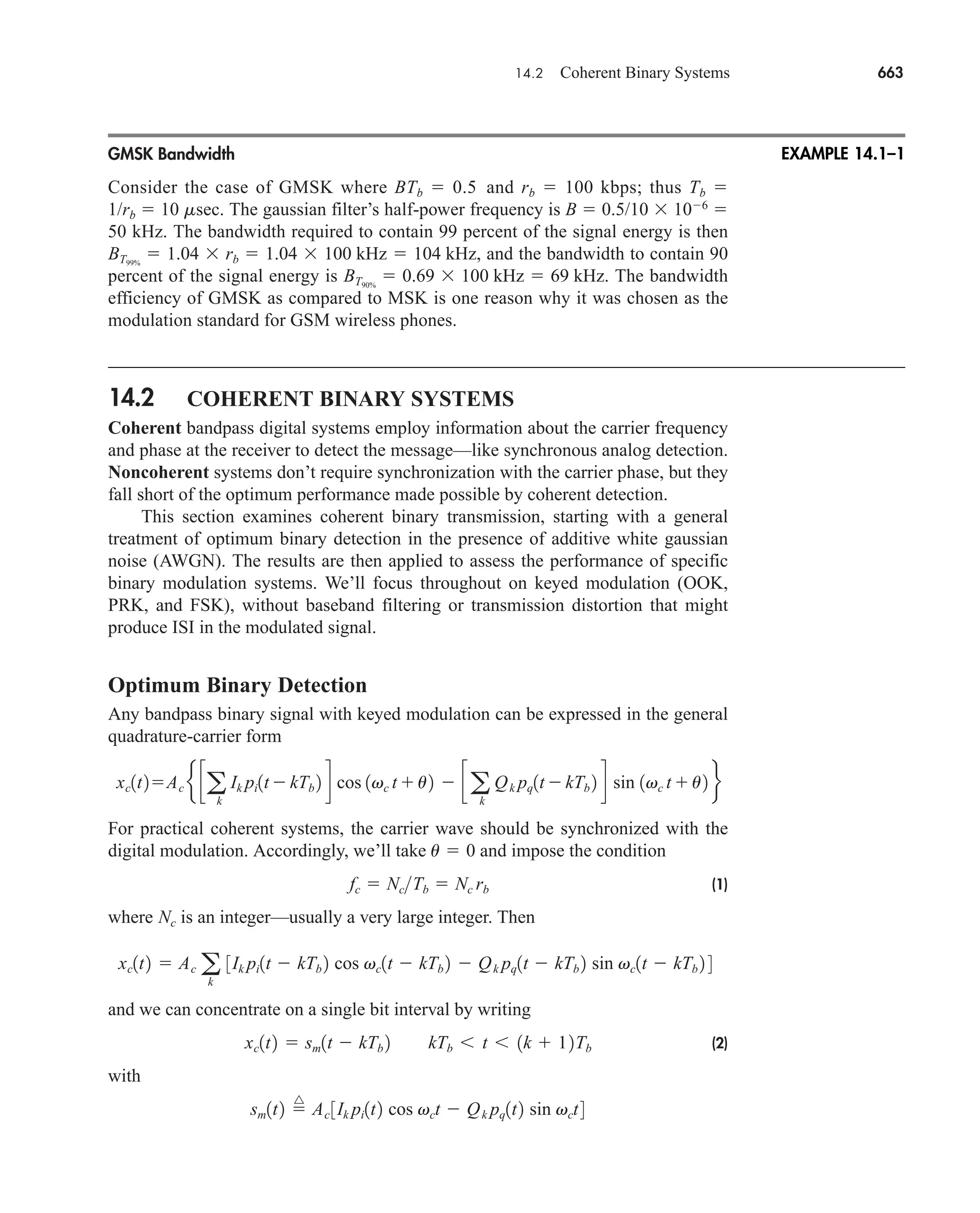
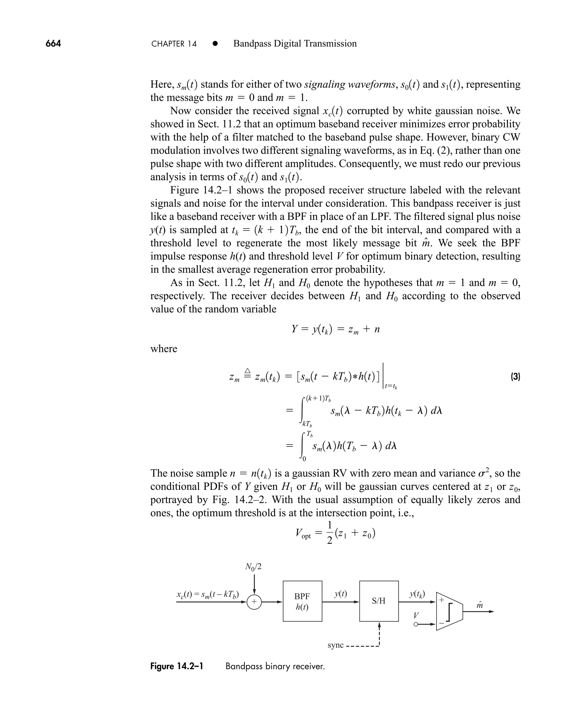
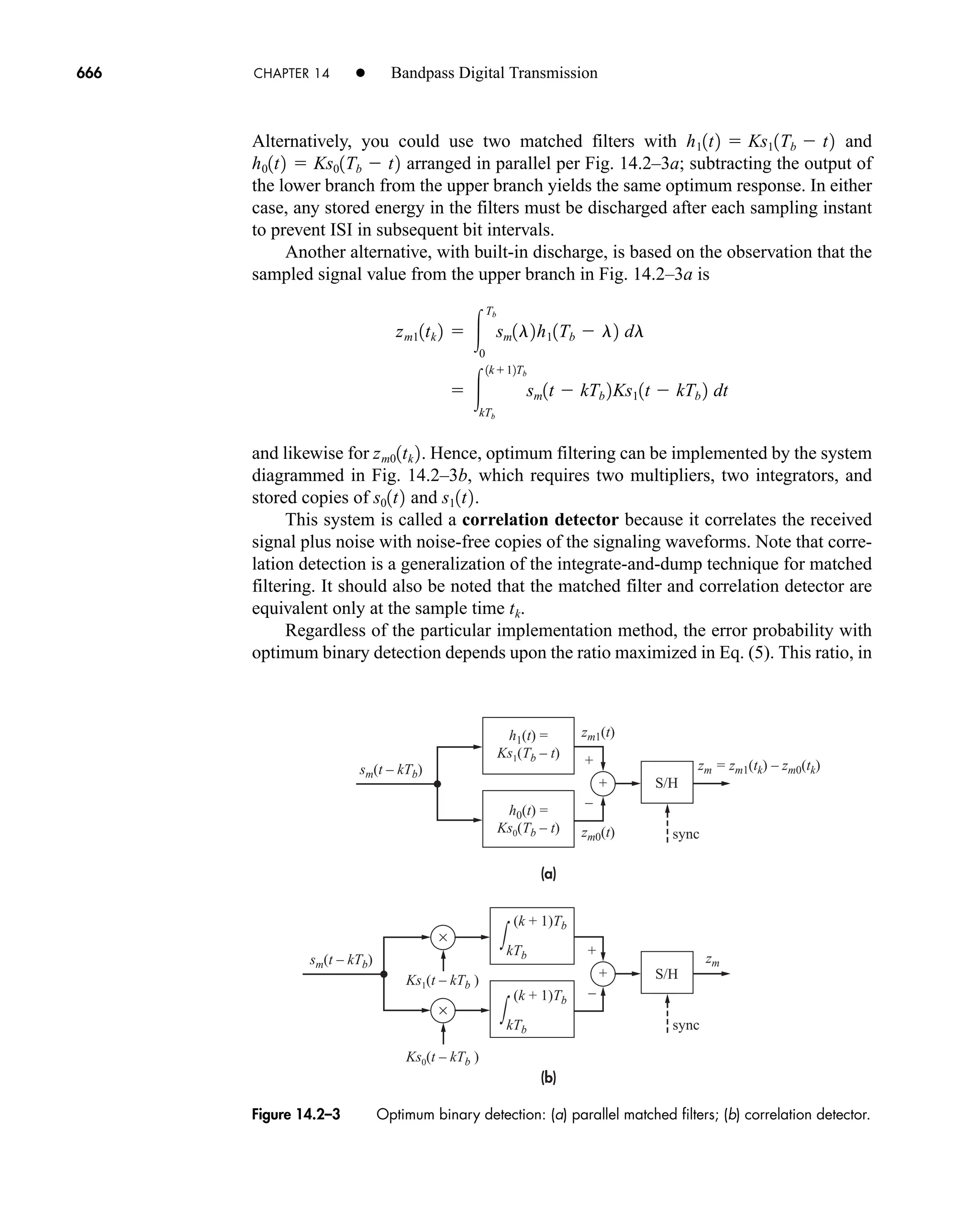
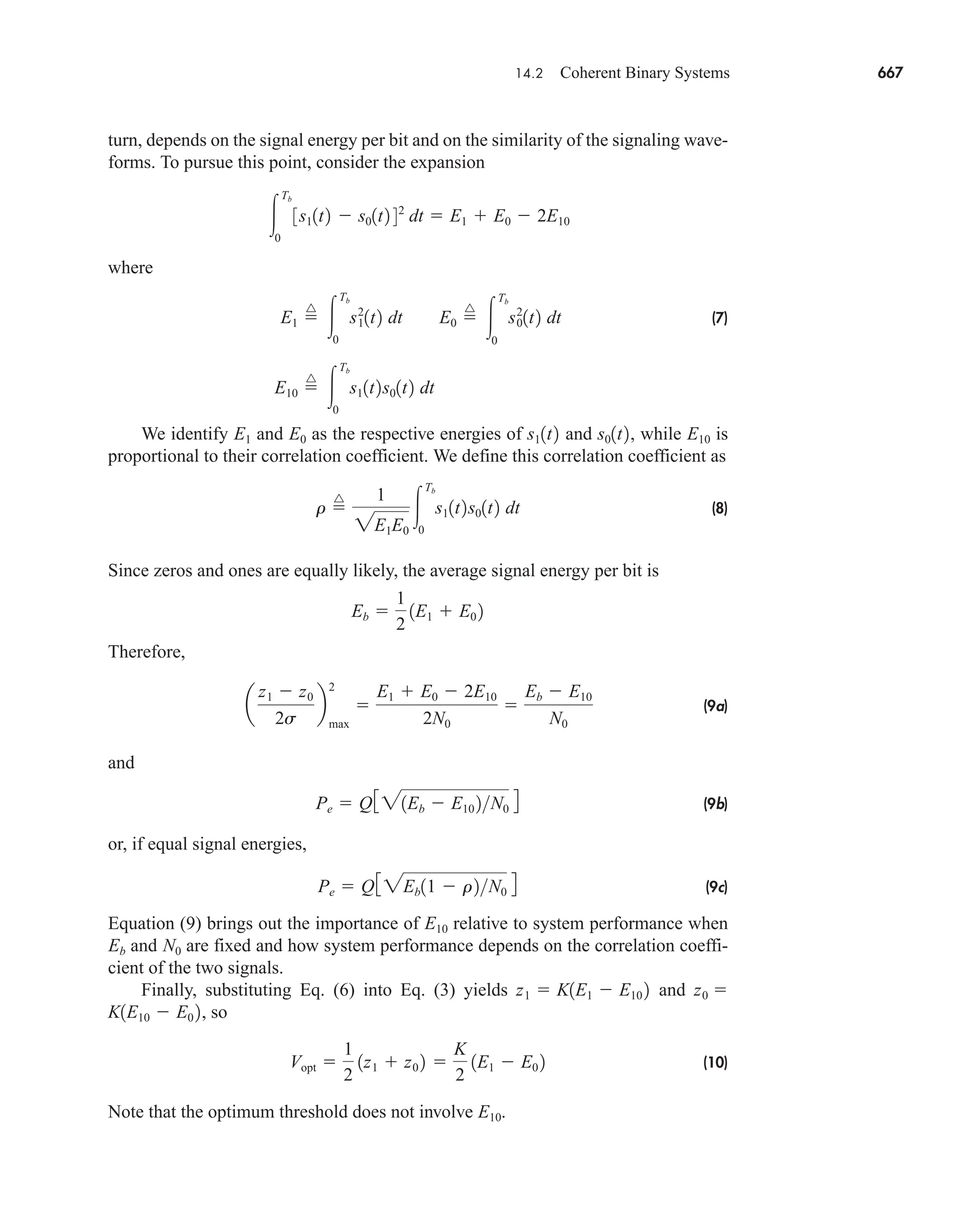
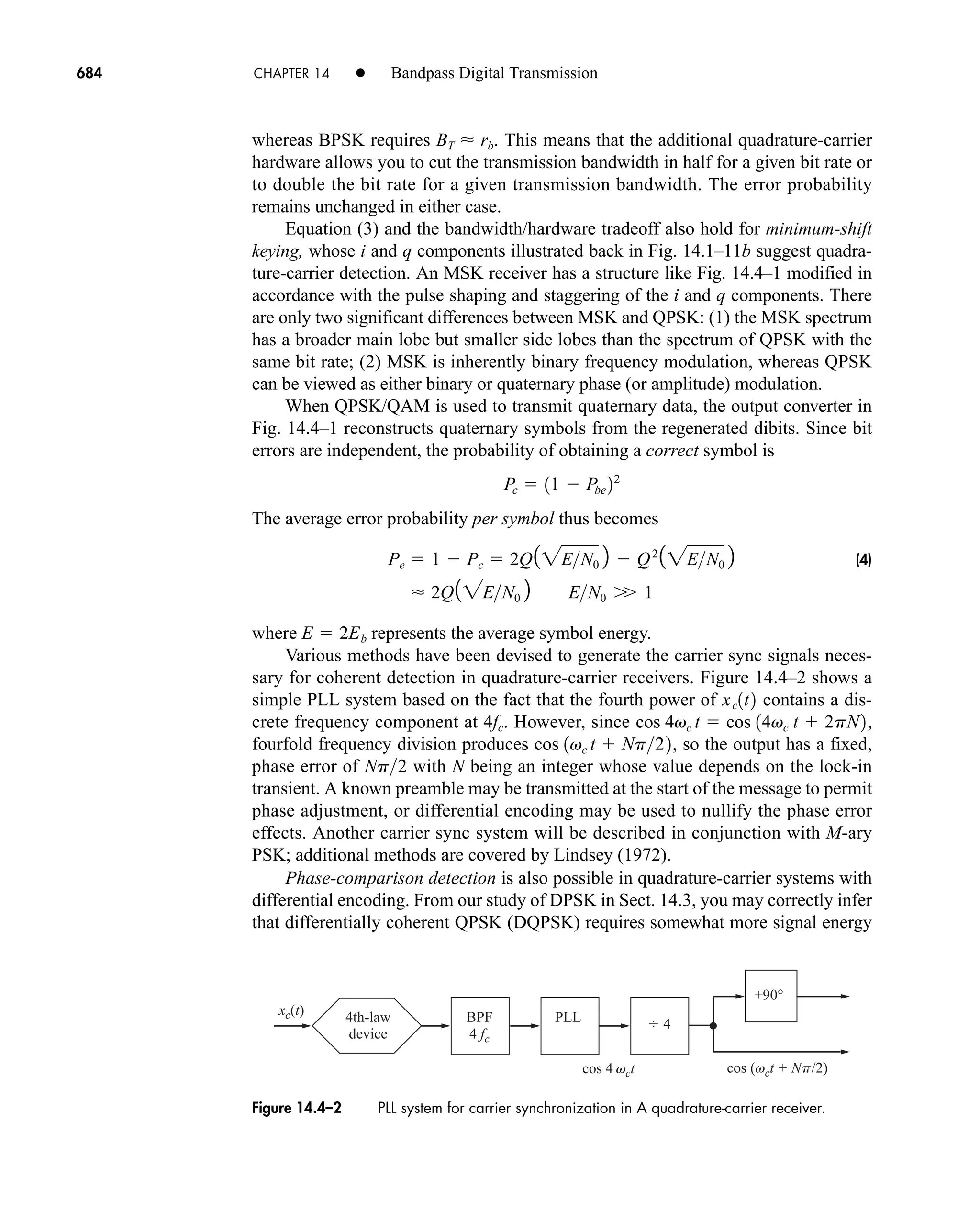
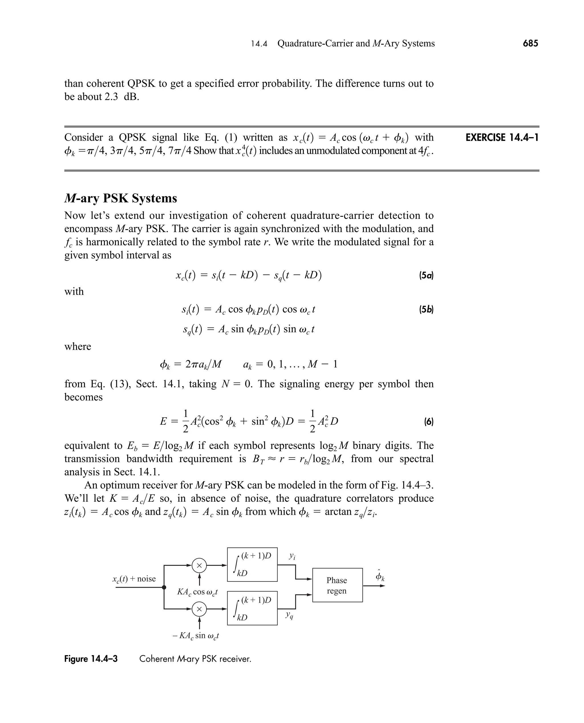
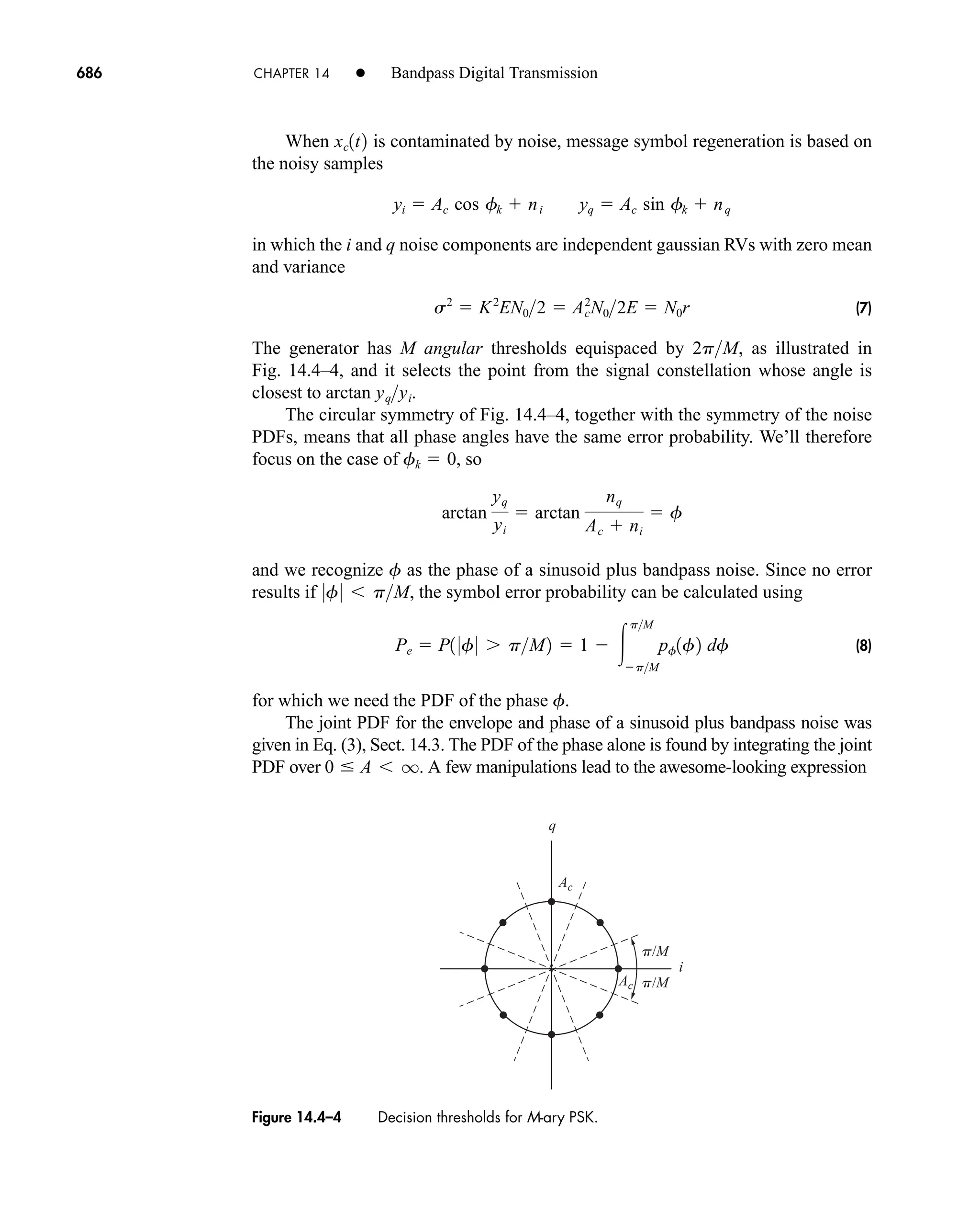
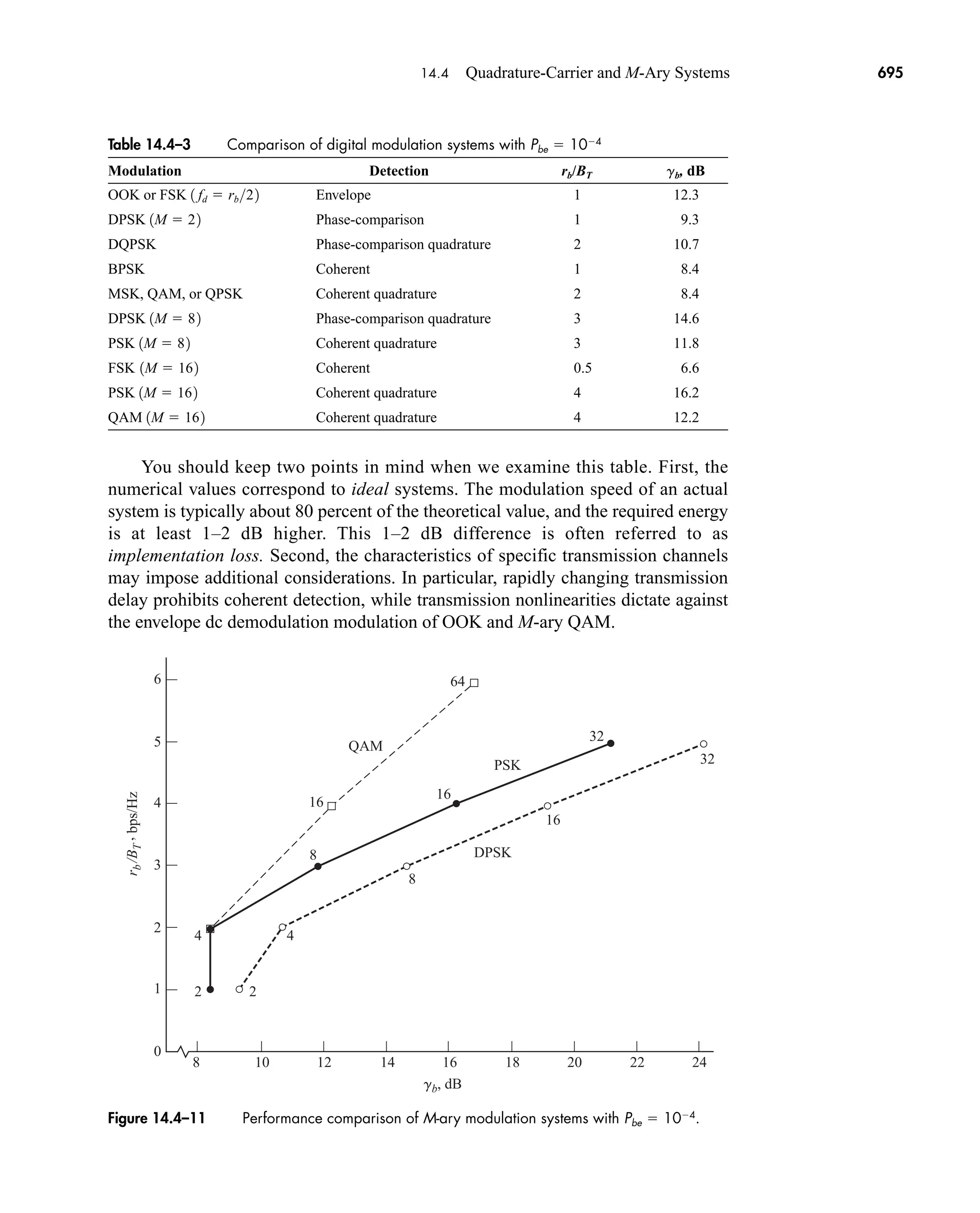
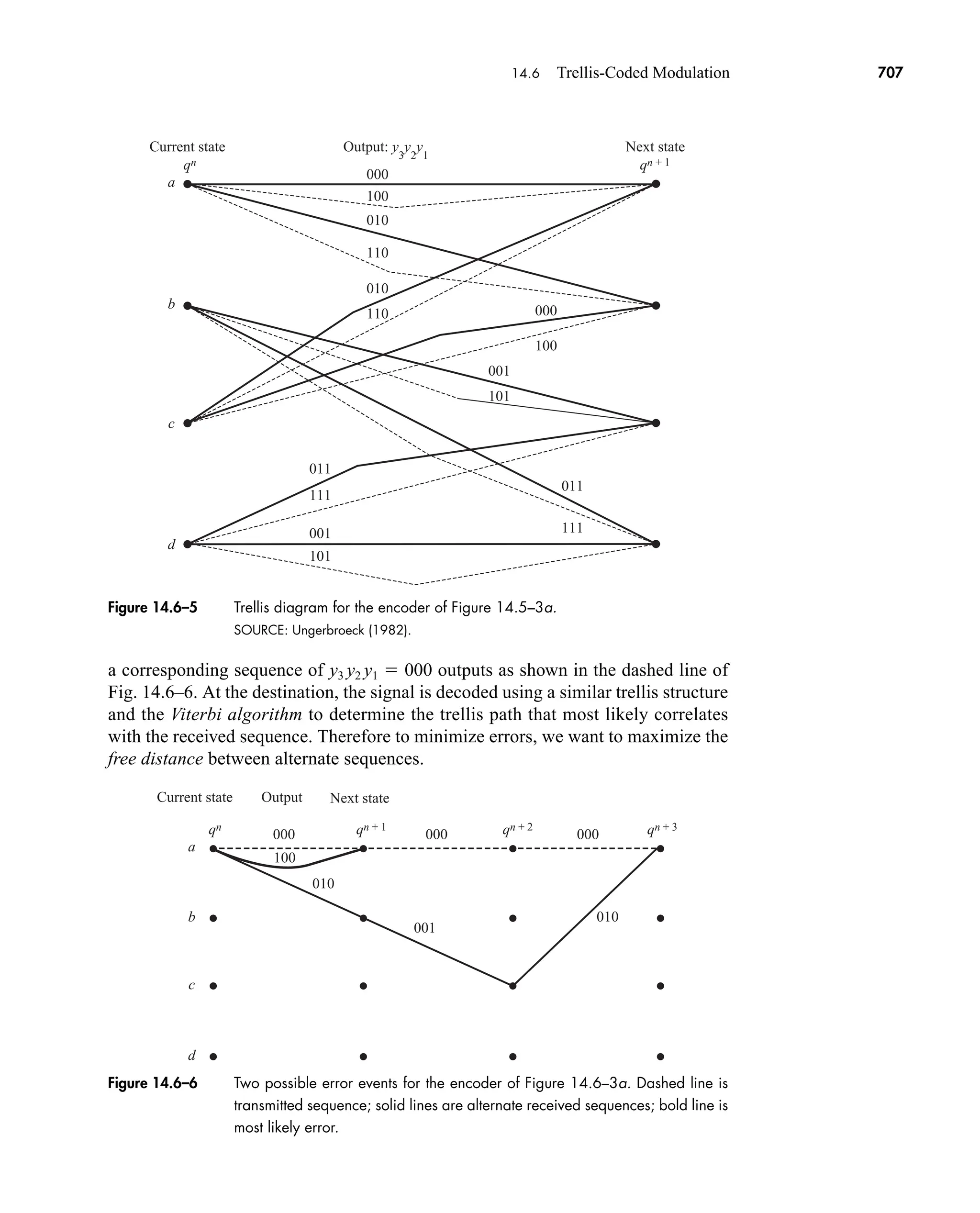
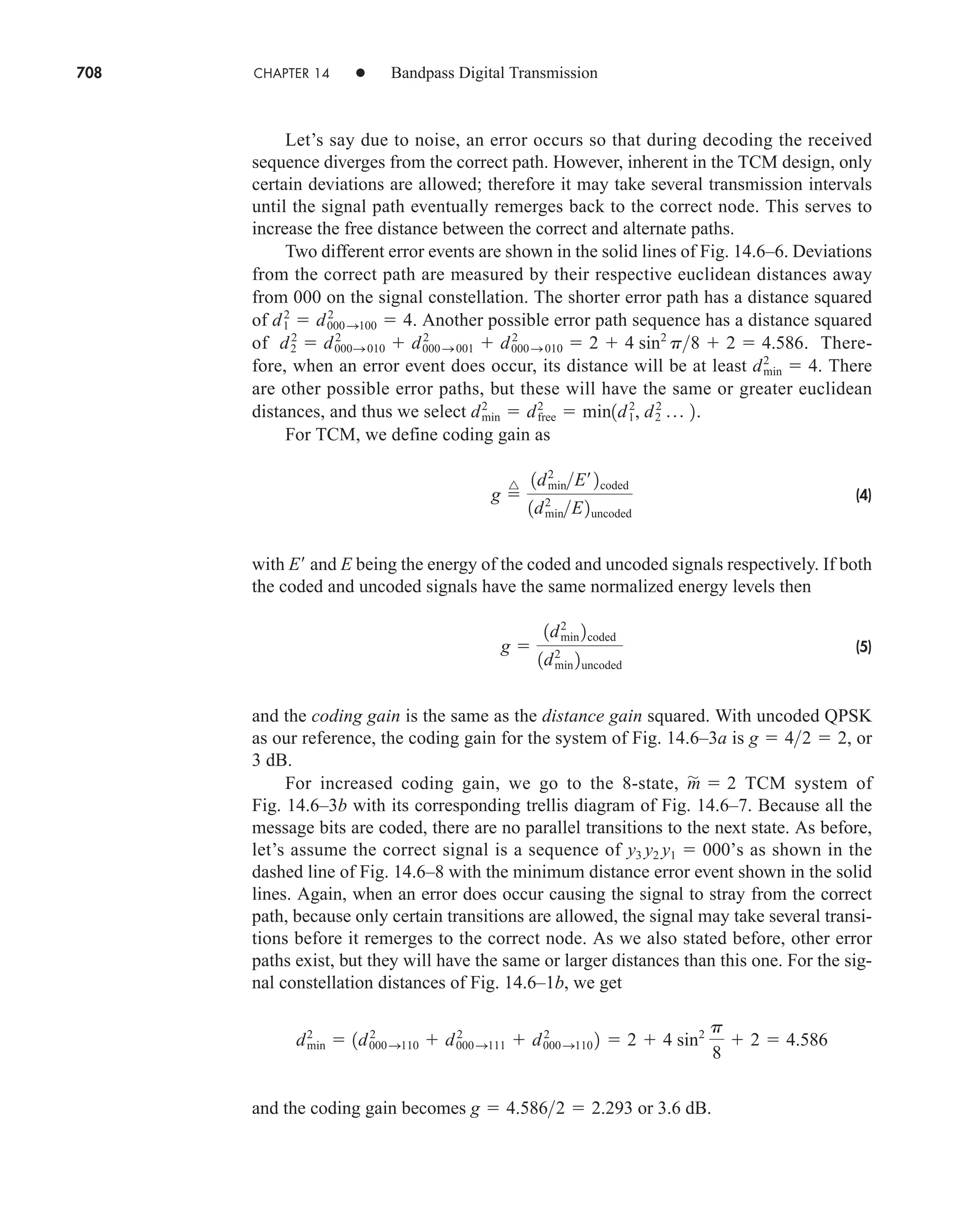
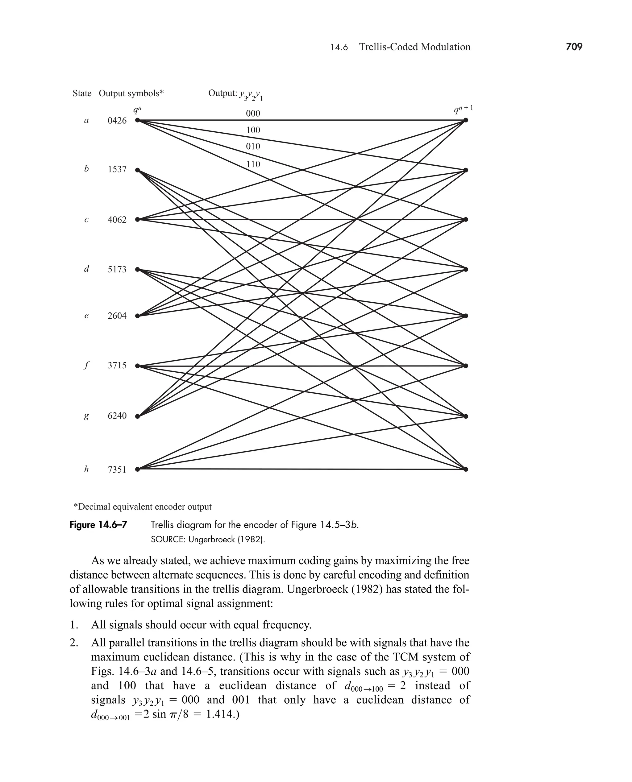
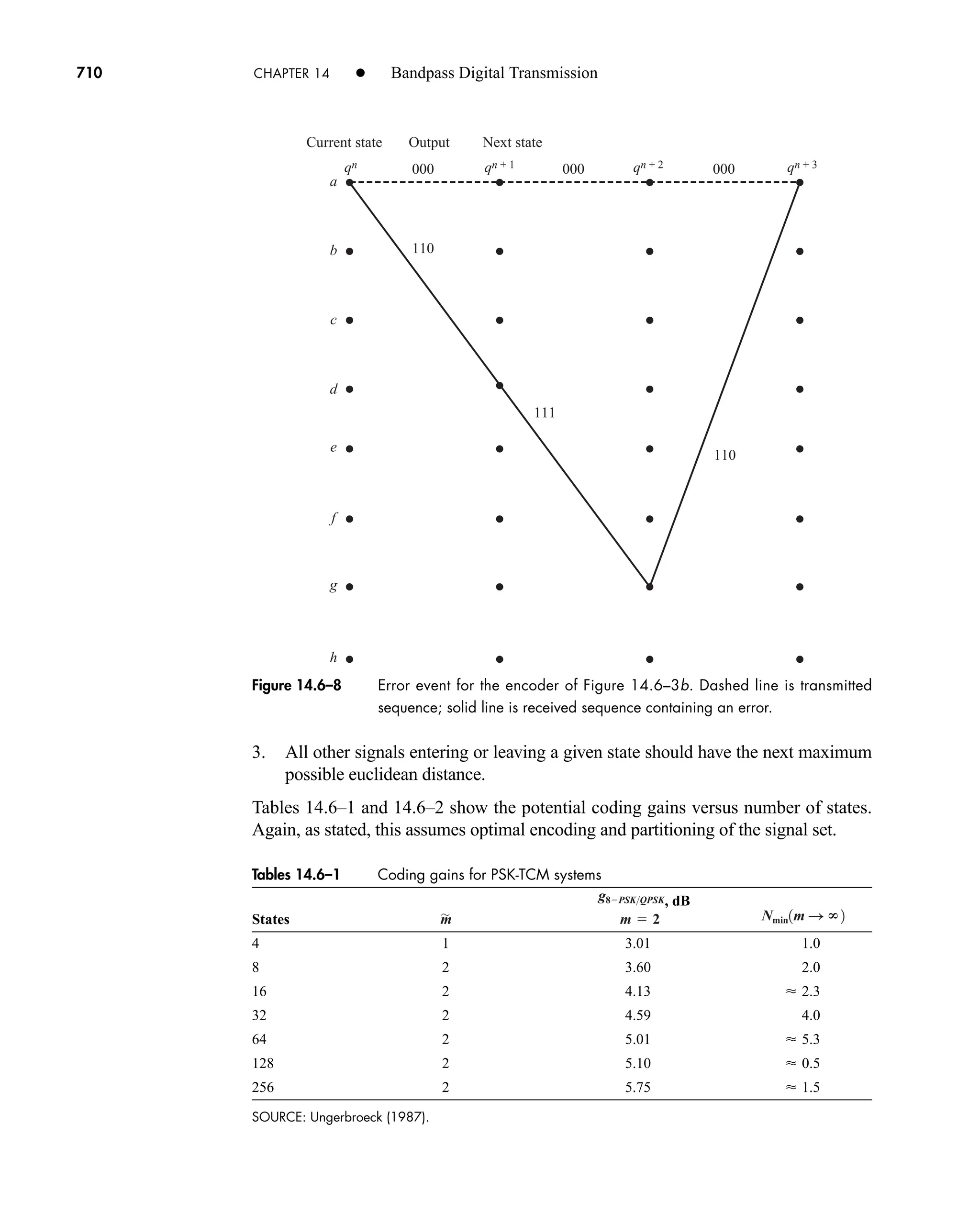
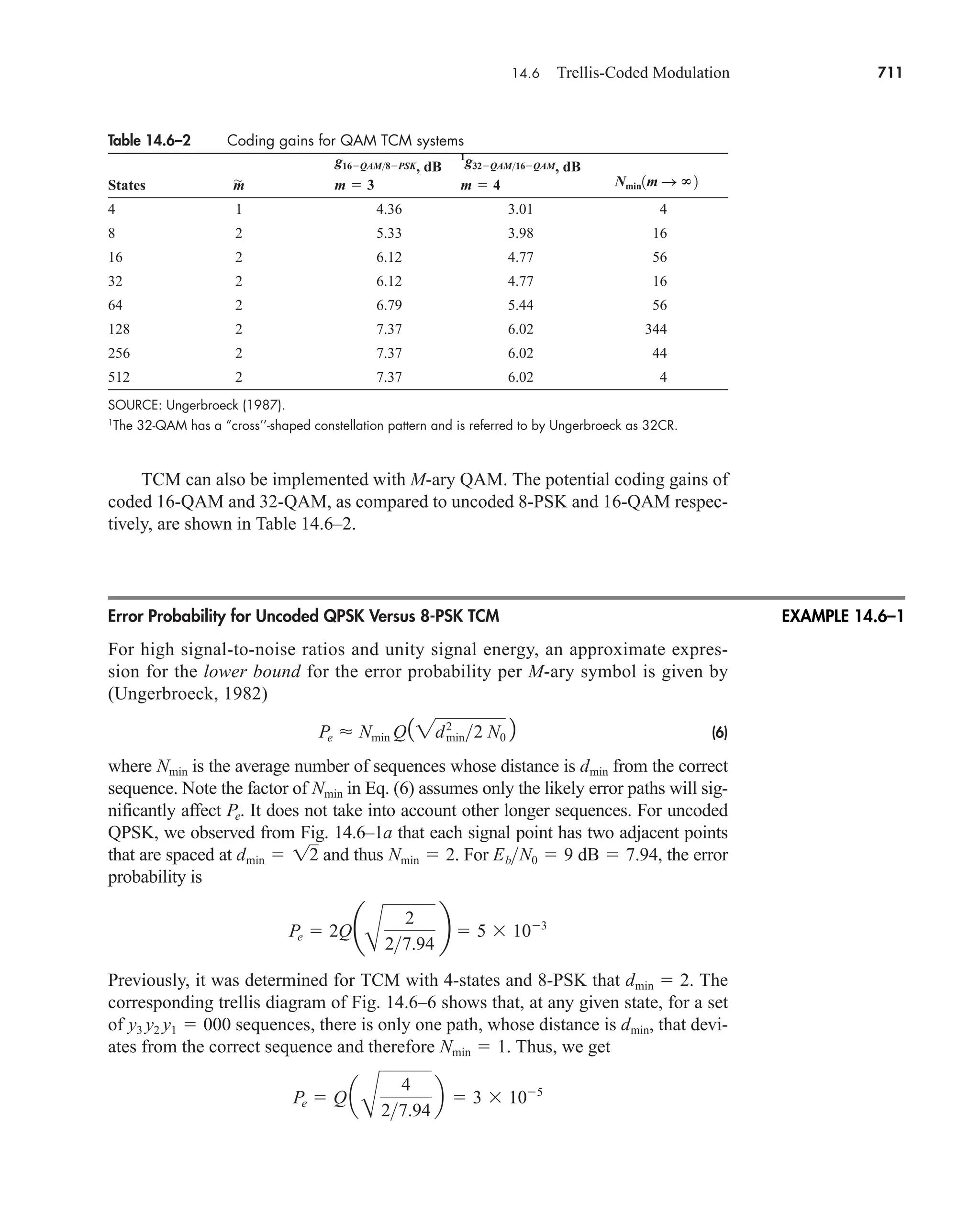
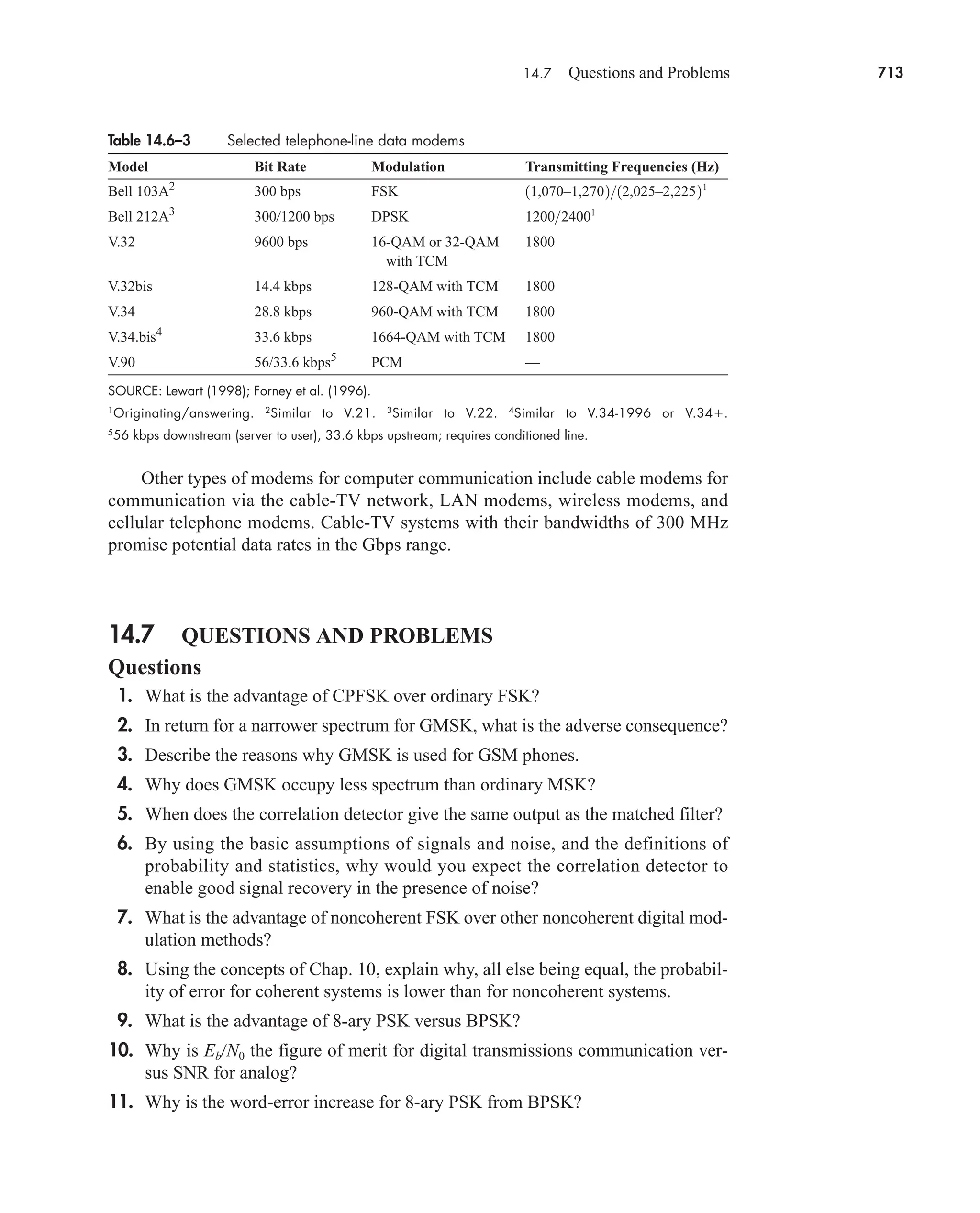
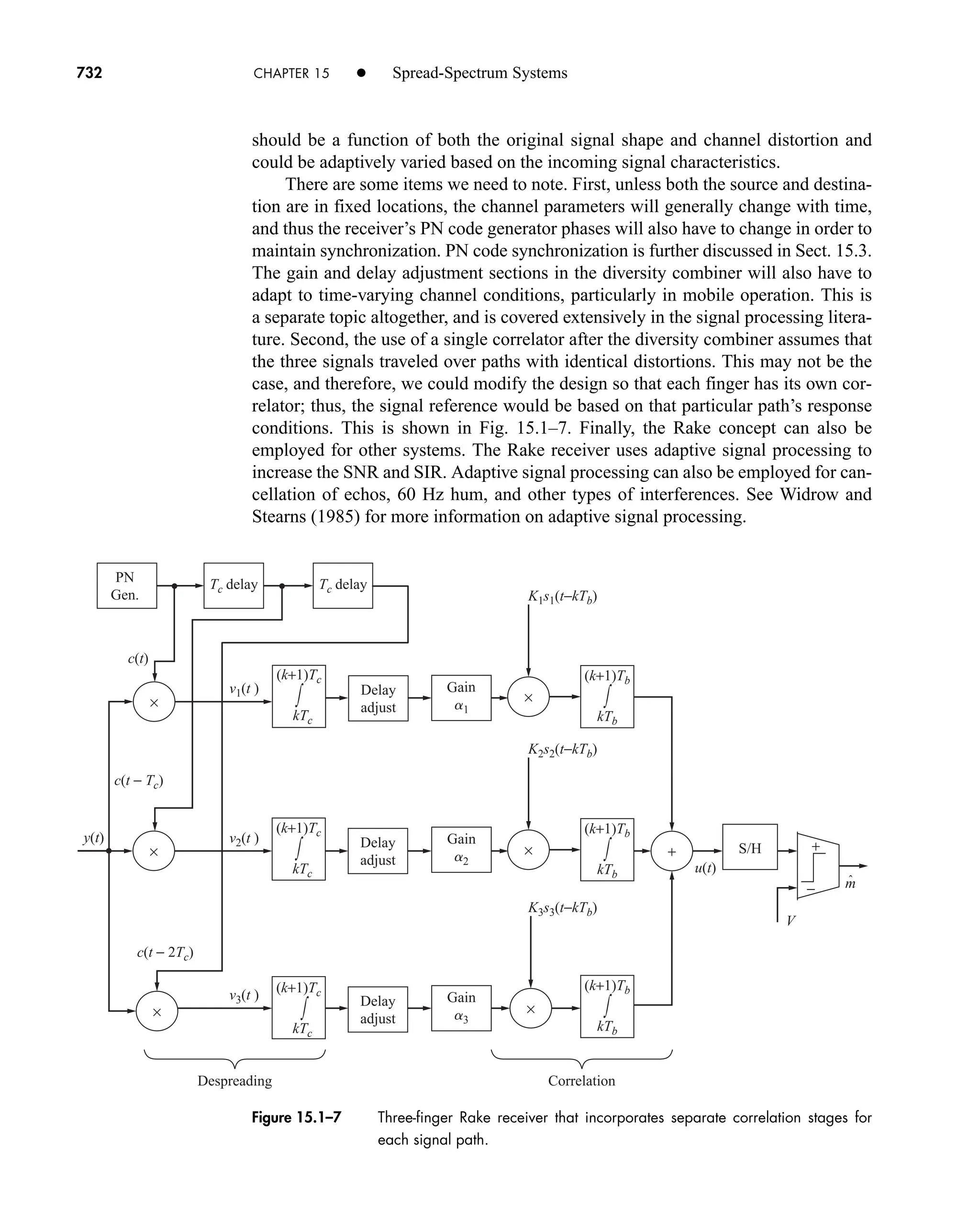
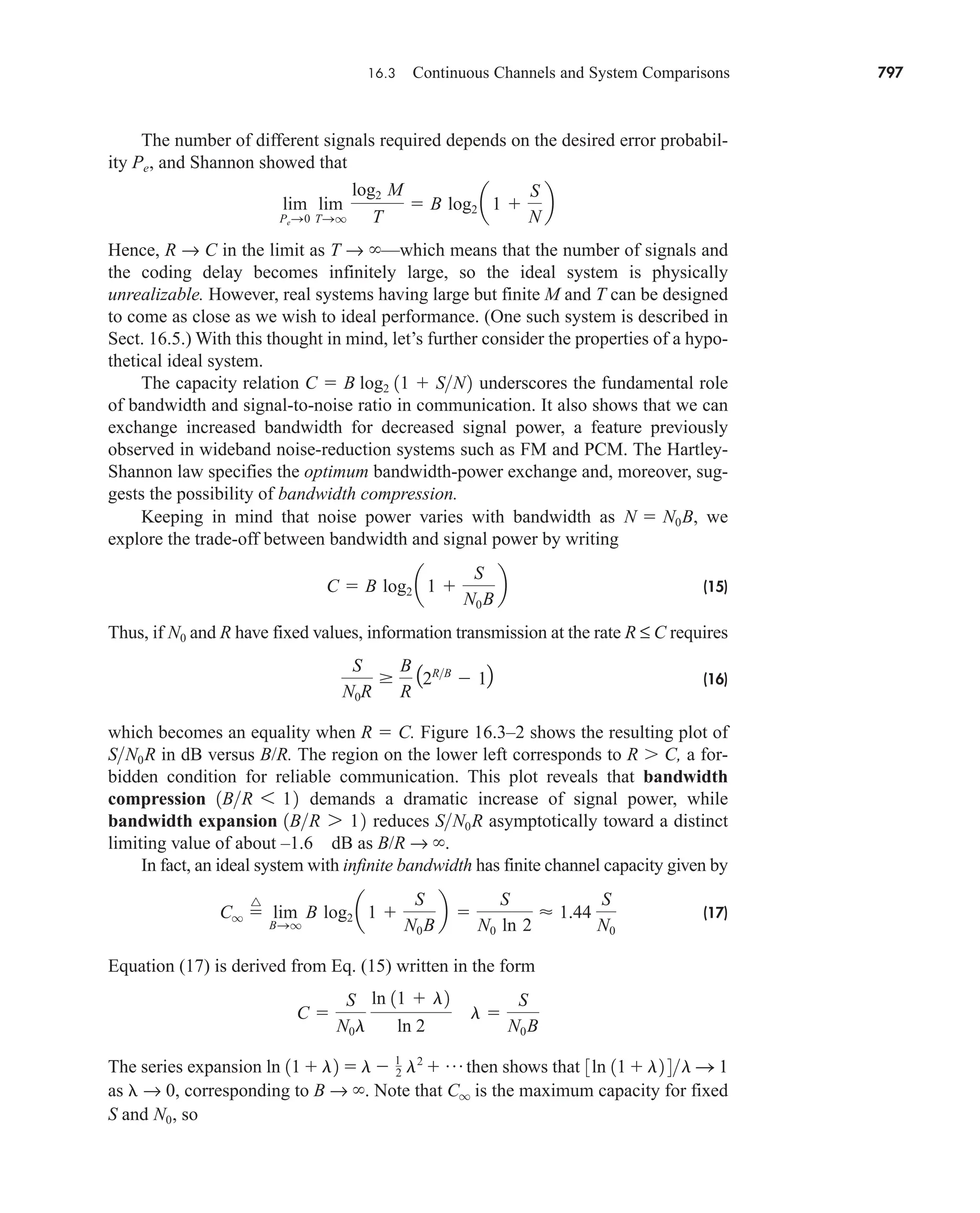
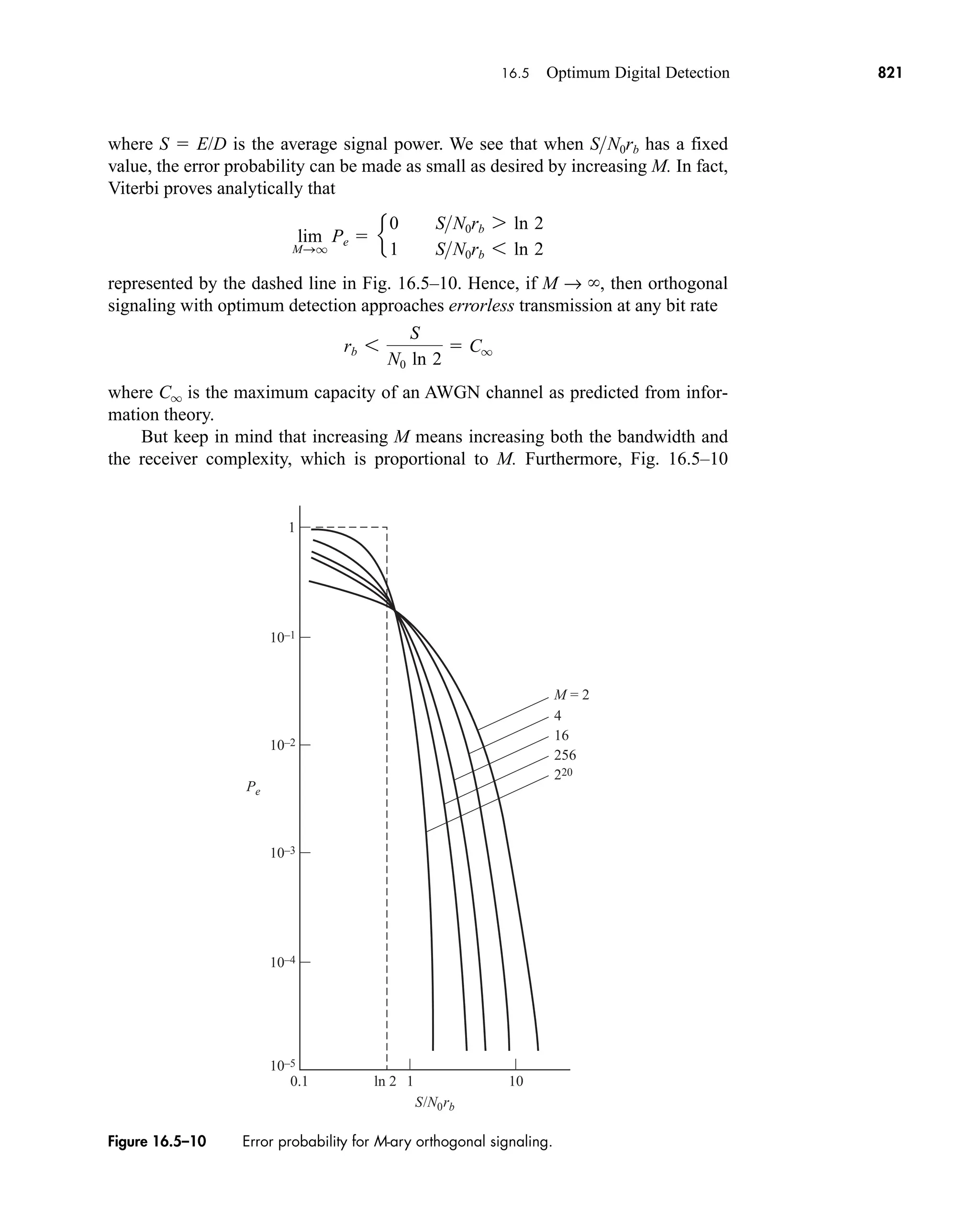
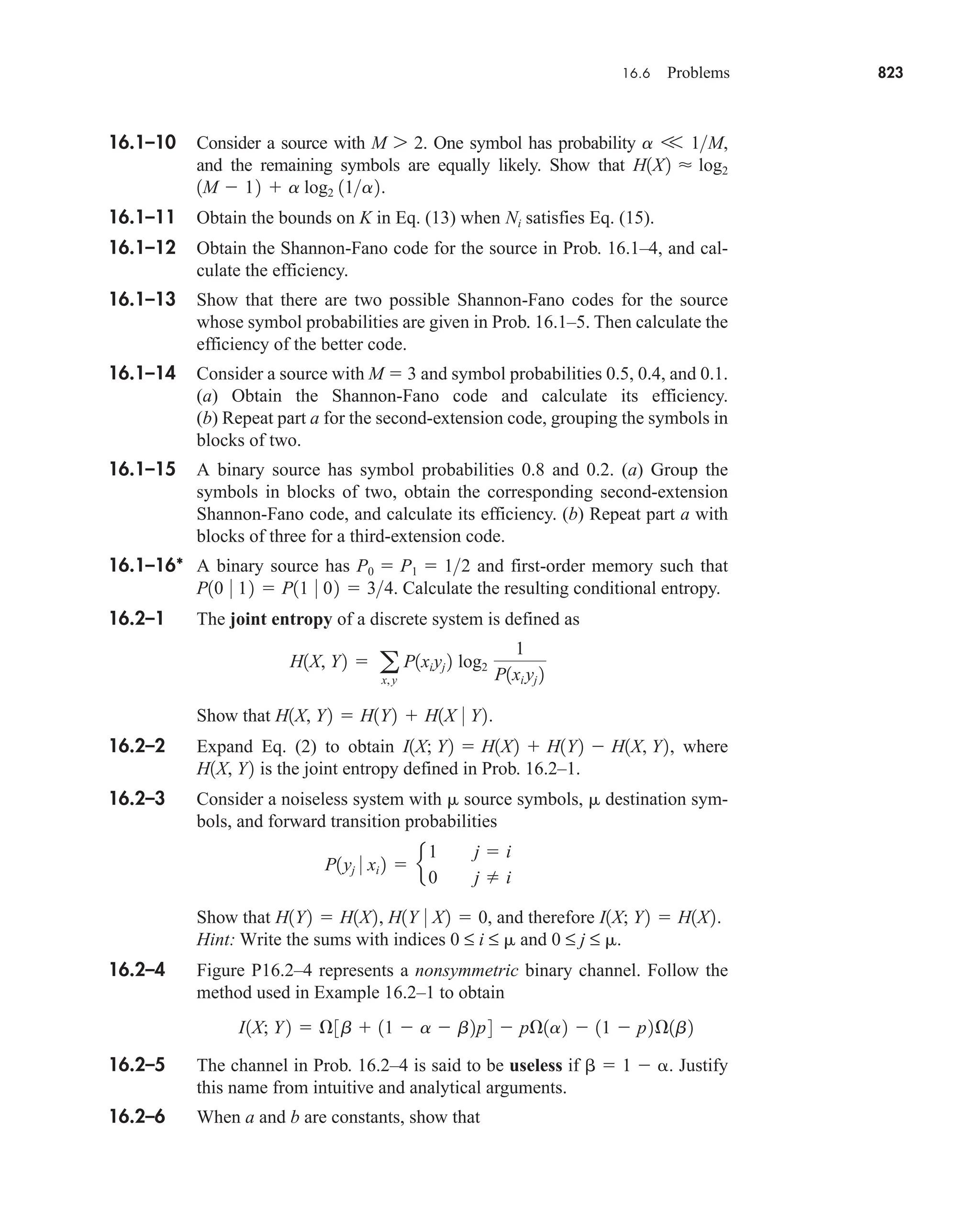
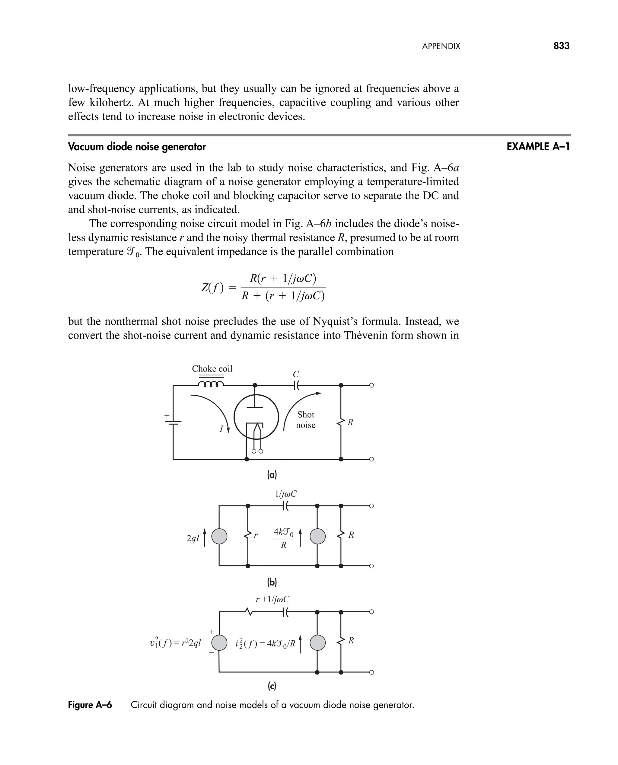
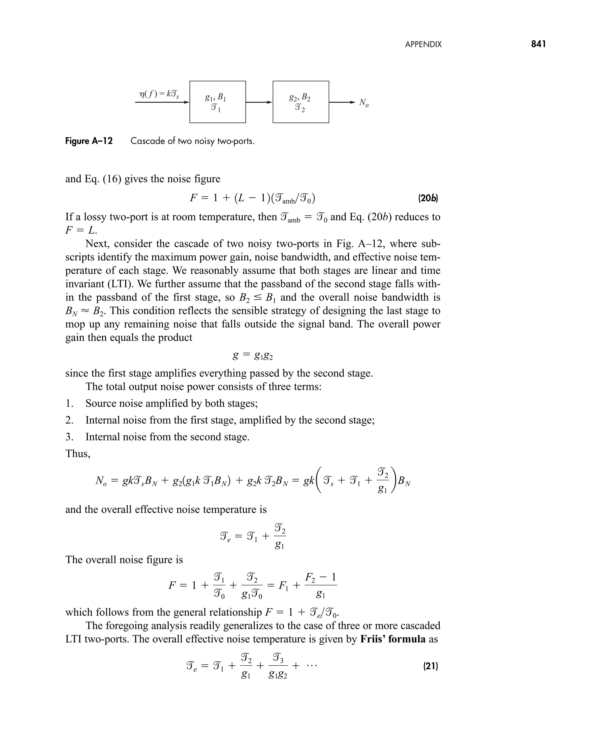
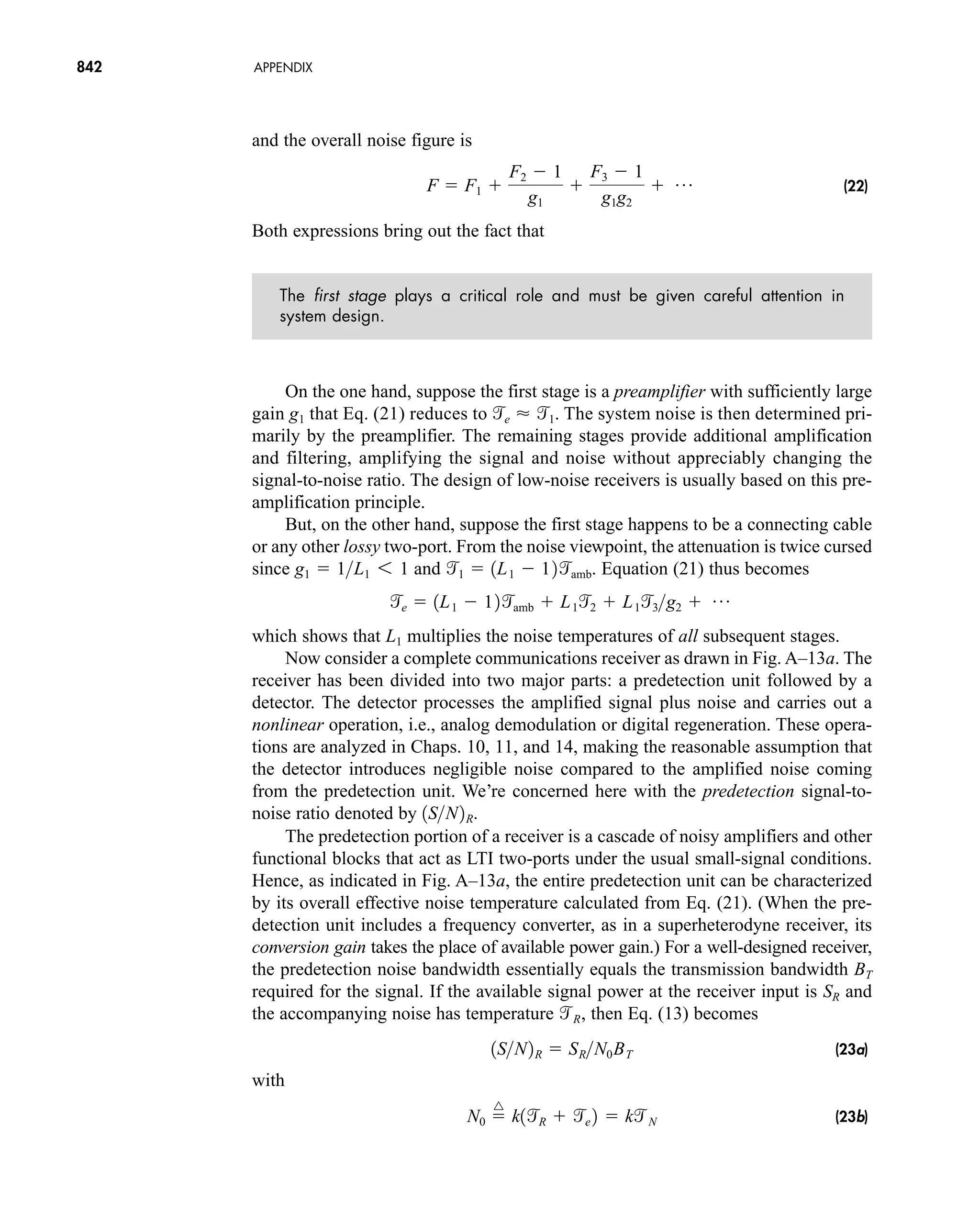
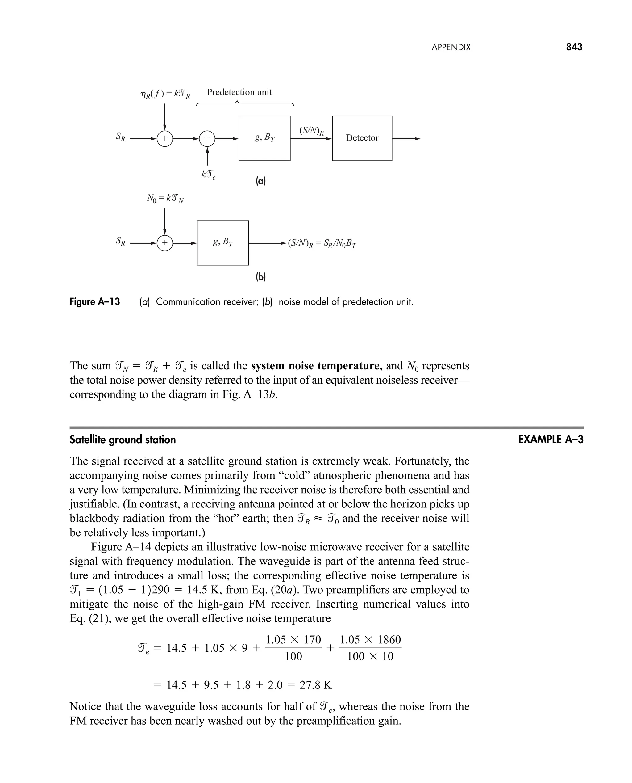
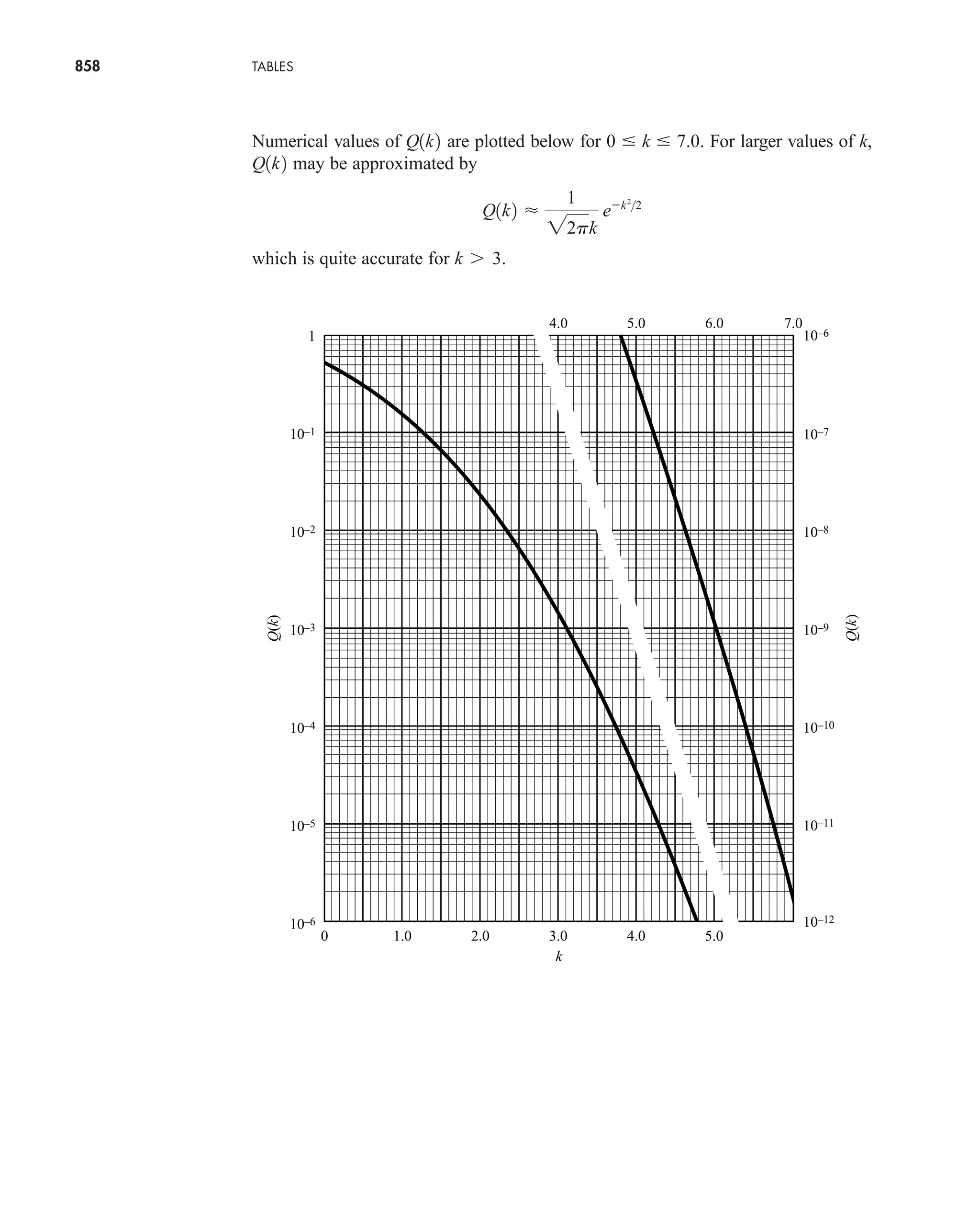
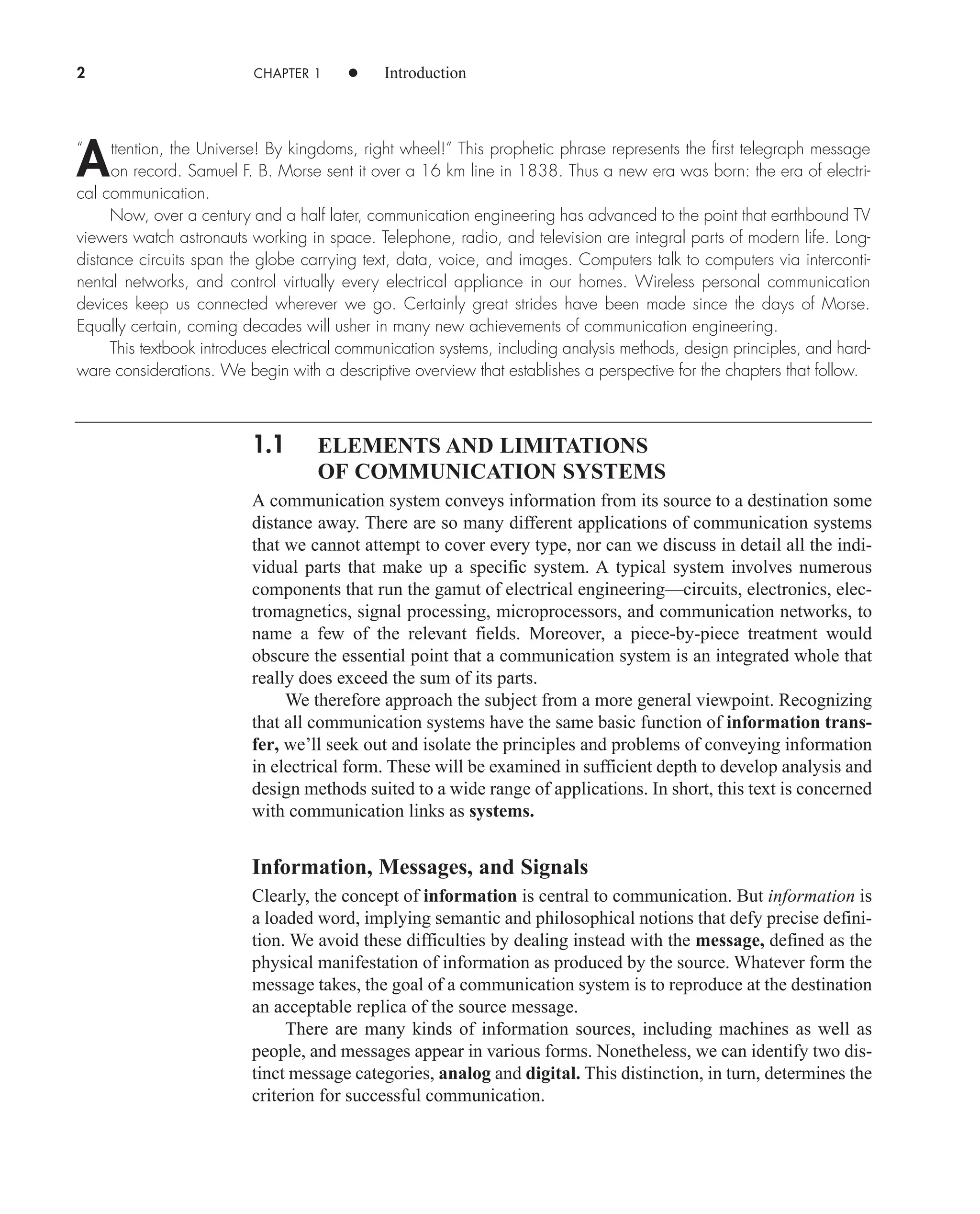
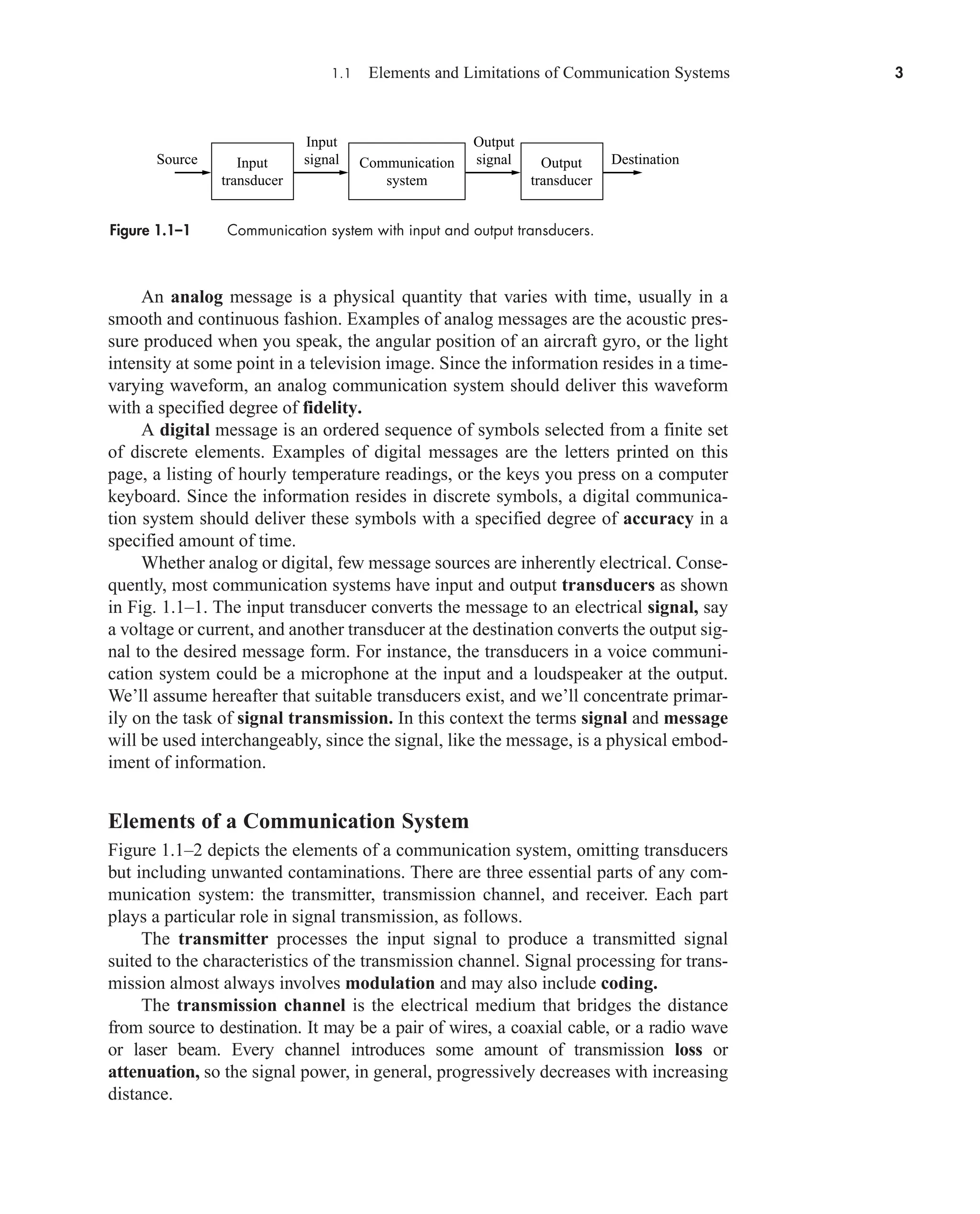
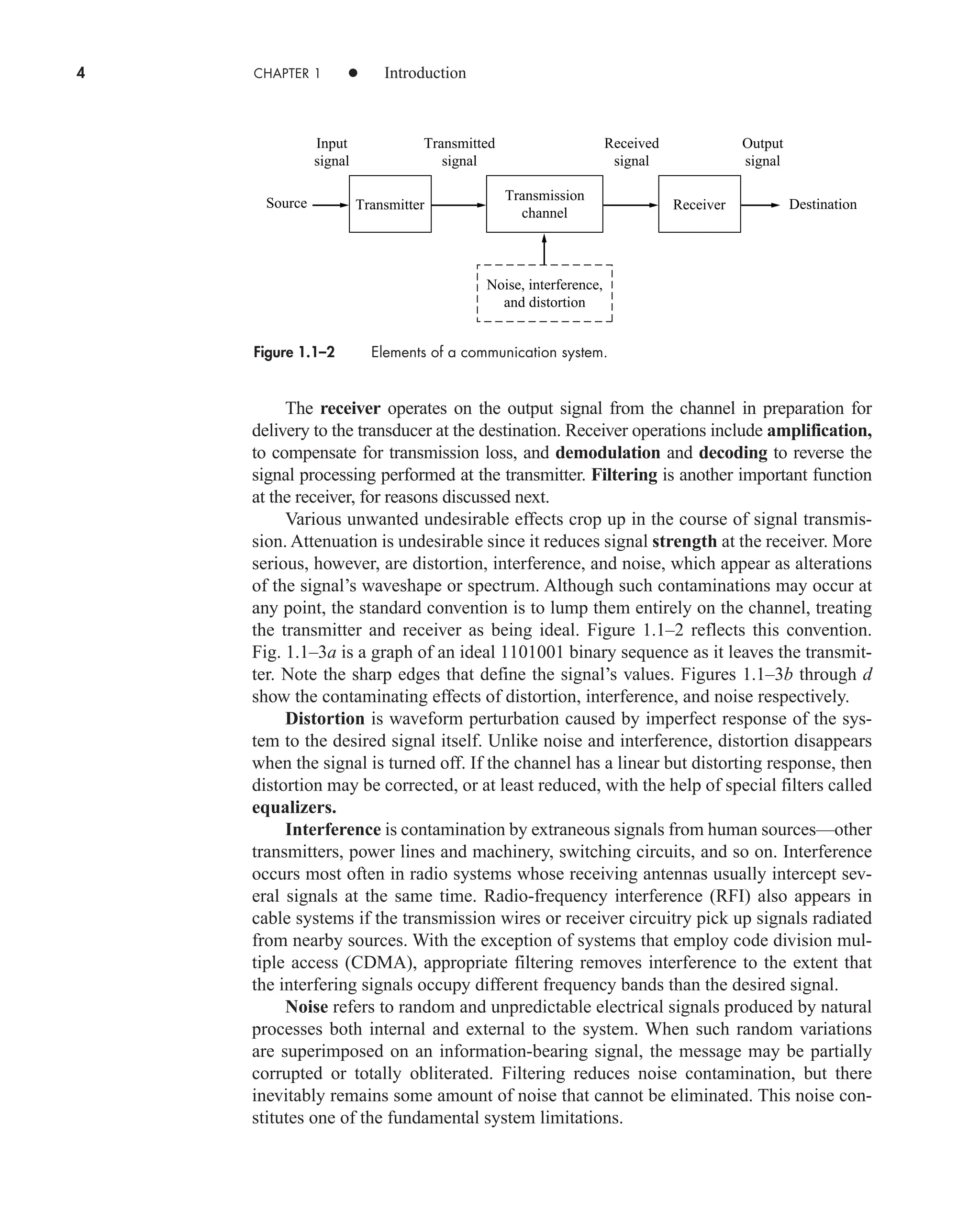
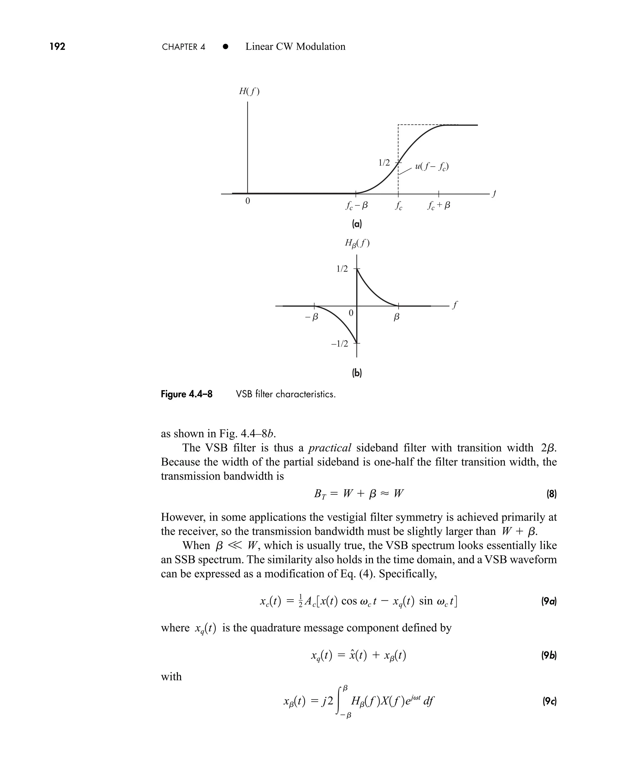
The document is the fifth edition of 'Communication Systems: An Introduction to Signals and Noise in Electrical Communication' by A. Bruce Carlson and Paul B. Crilly, published by McGraw-Hill. It covers various topics in communication systems, including signal theory, modulation, transmission, noise, and digital communication techniques. The book serves as a comprehensive resource for understanding the principles and developments in electrical communication.


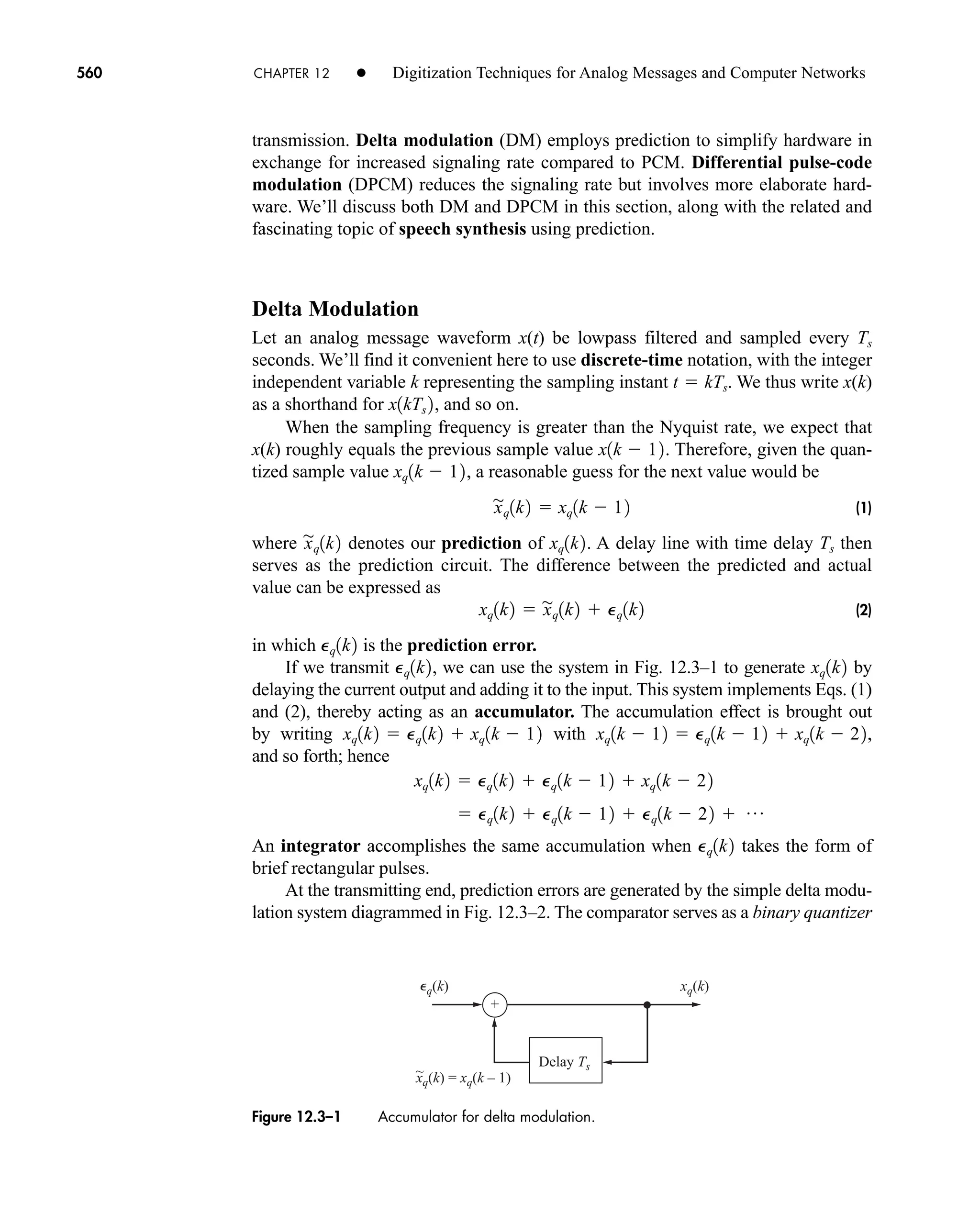
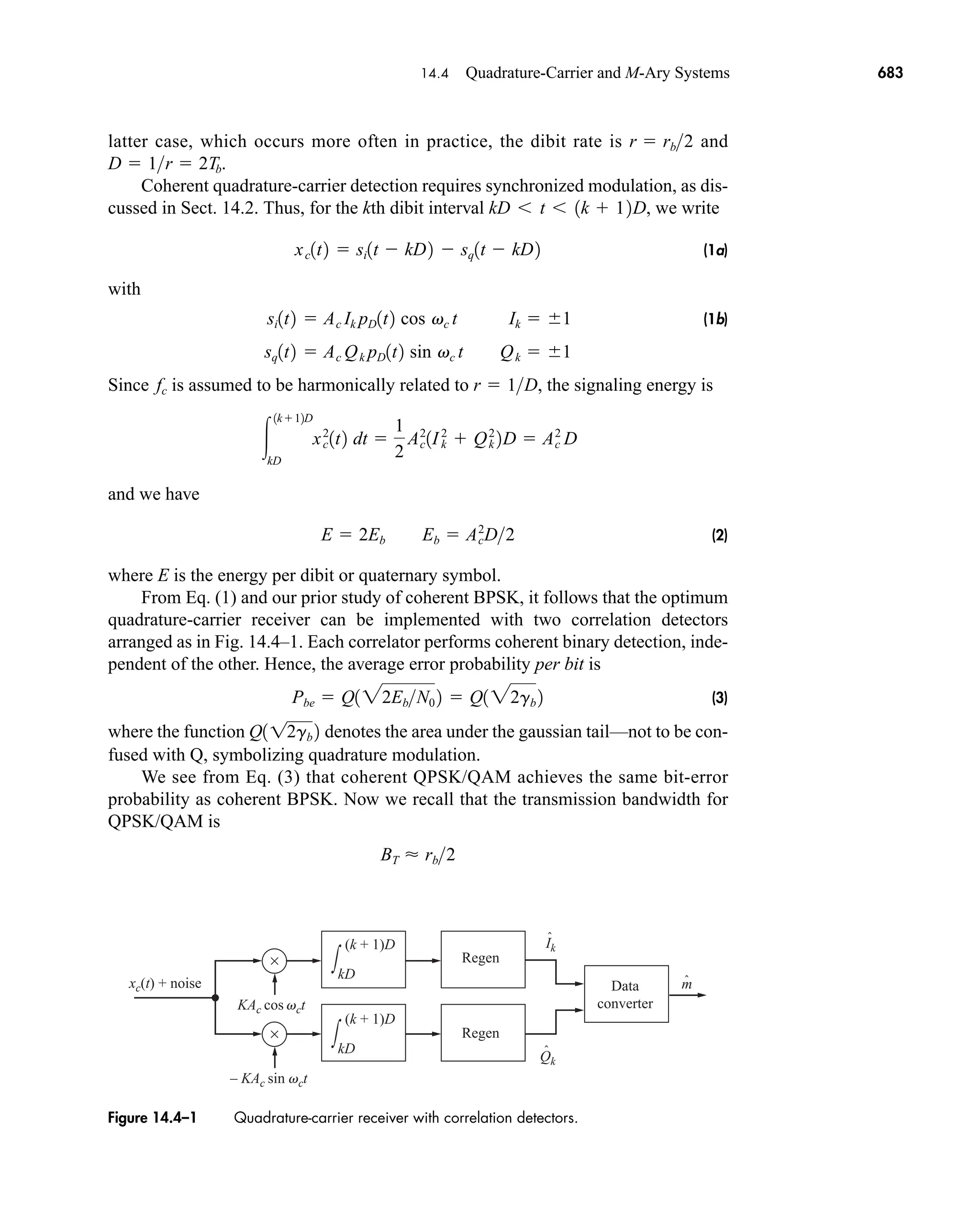
![xvii
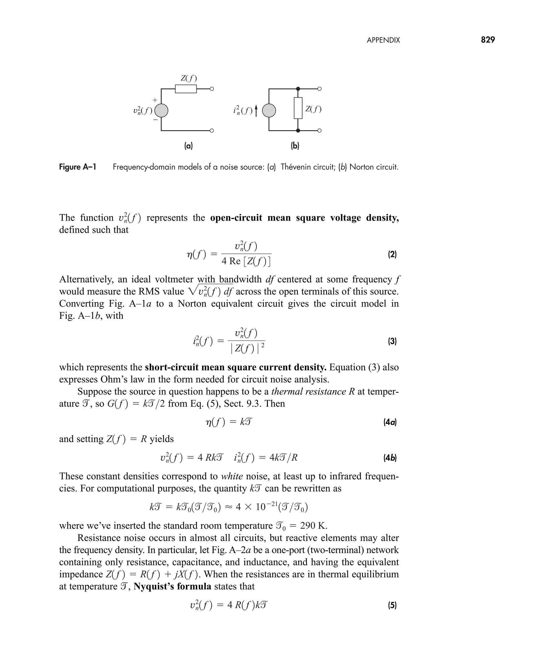
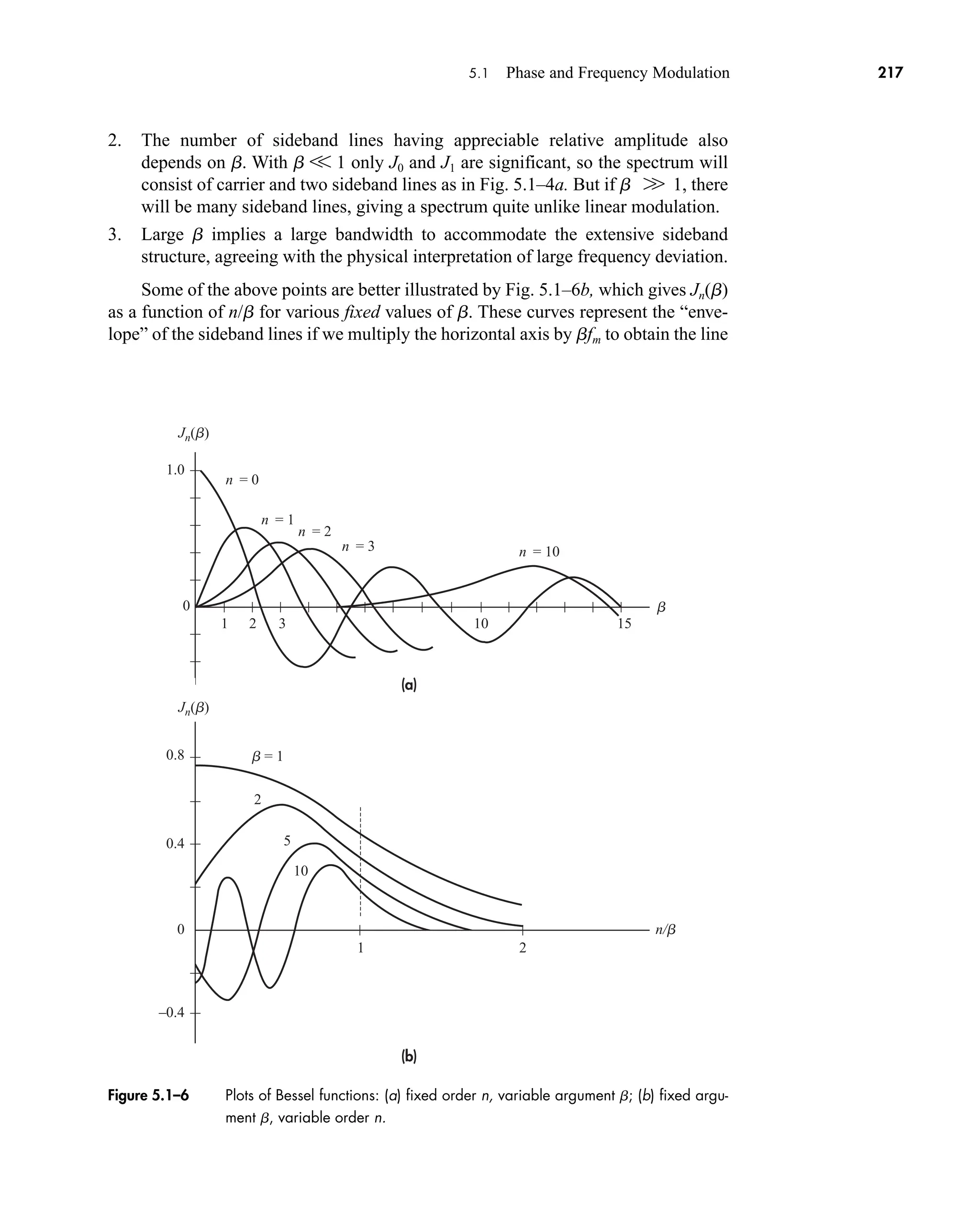
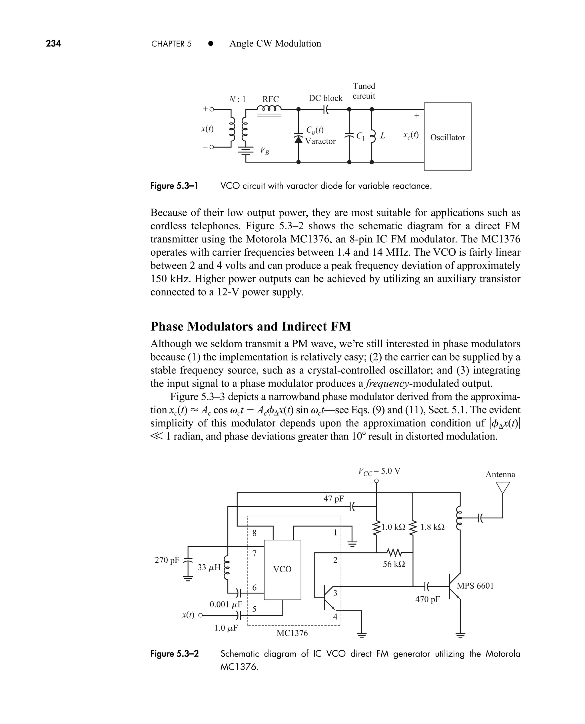
Mathematical Symbols
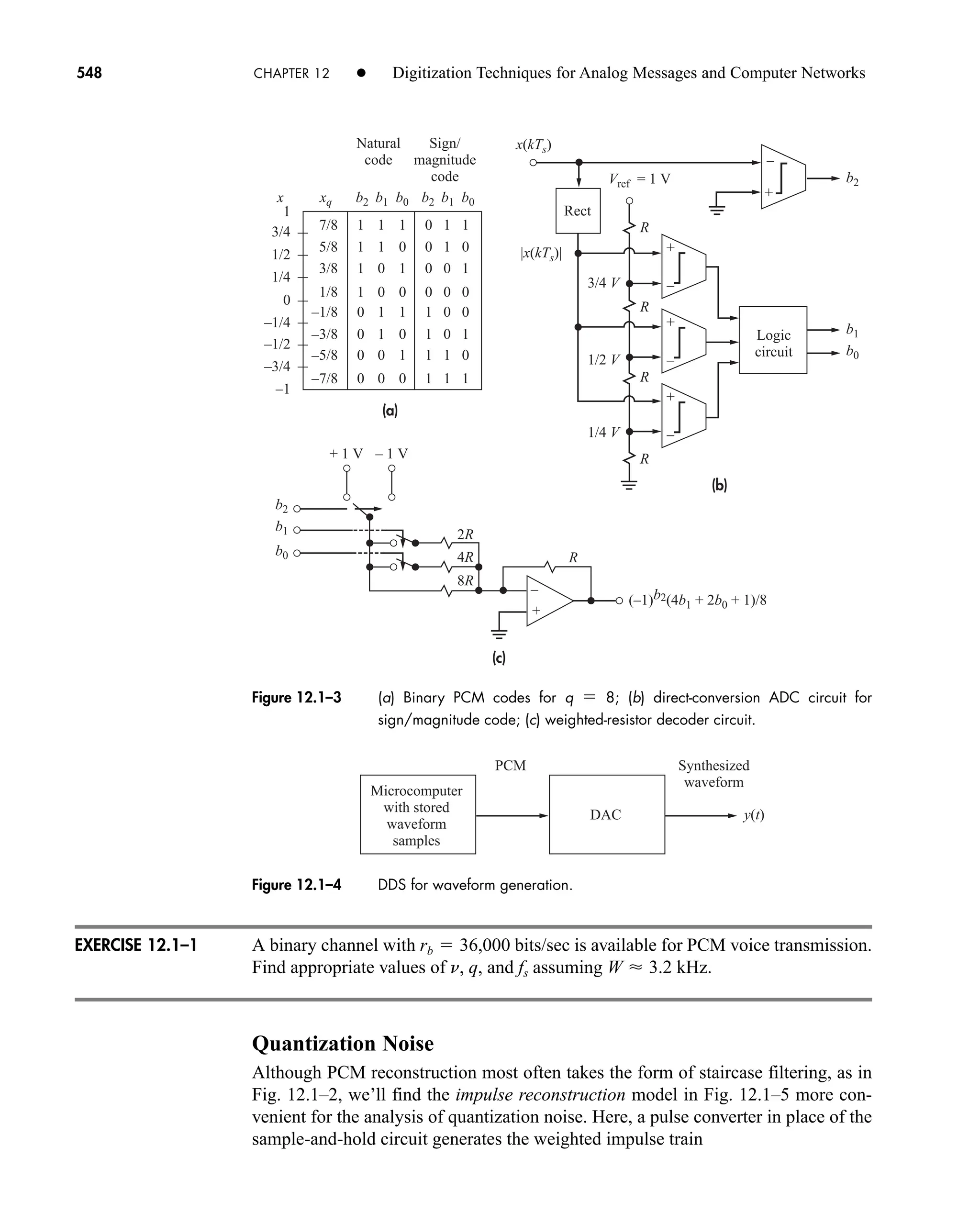
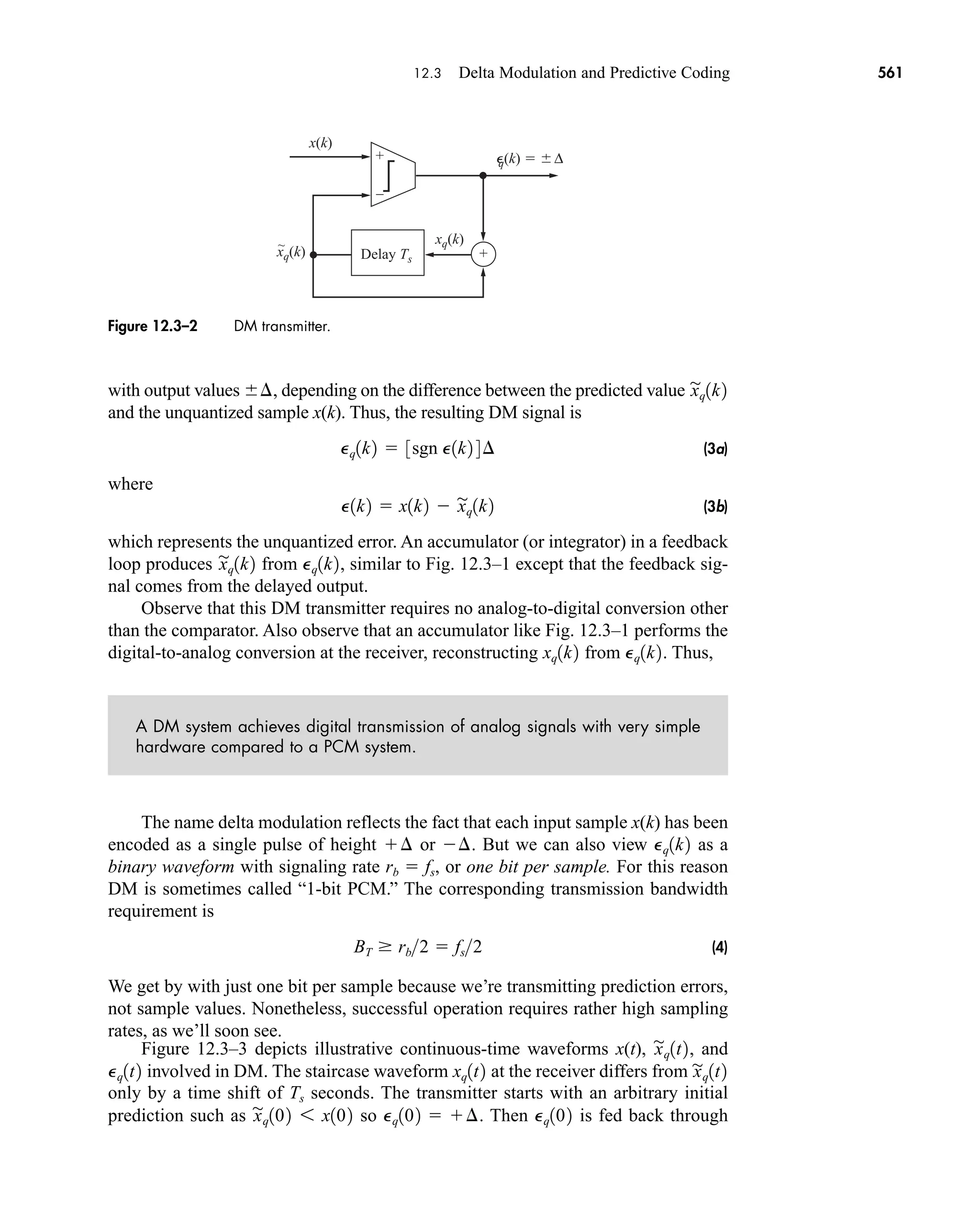
A, Ac amplitude constant and carrier amplitude constant
Ae aperture area
Am tone amplitude
Av(t) envelope of a BP signal
B bandwidth in hertz (Hz)
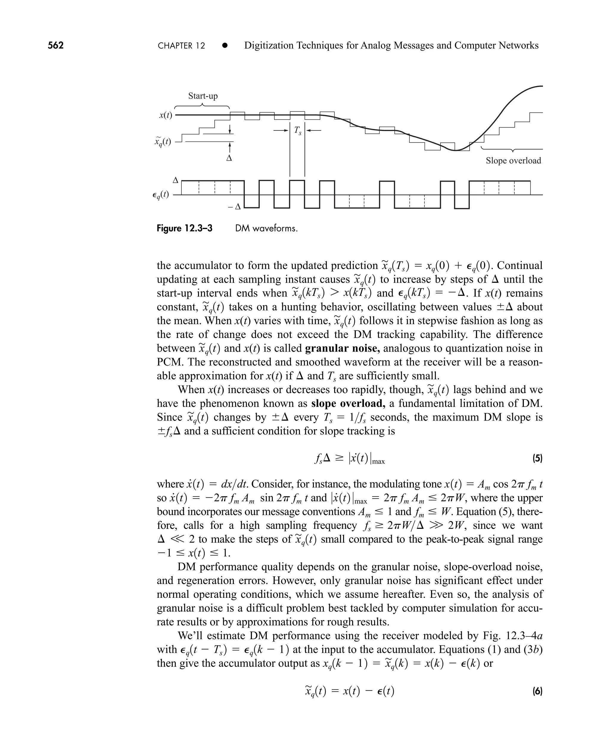
BT transmission bandwidth, or bandwidth of a bandpass signal
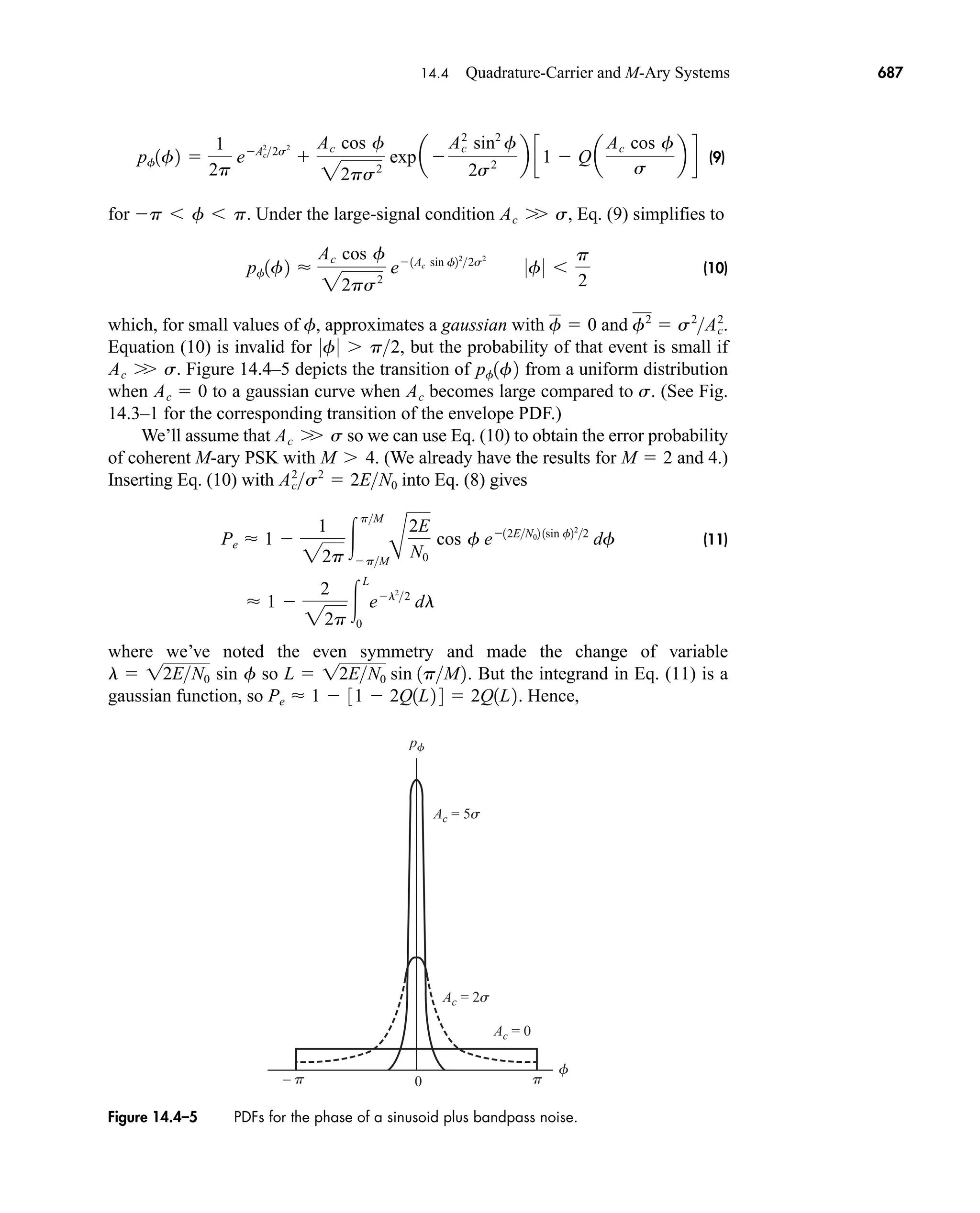
C channel capacity, bits per second, capacitance in Farads, or check vector
Cvw(t1, t2) covariance function of signals v(t) and w(t)
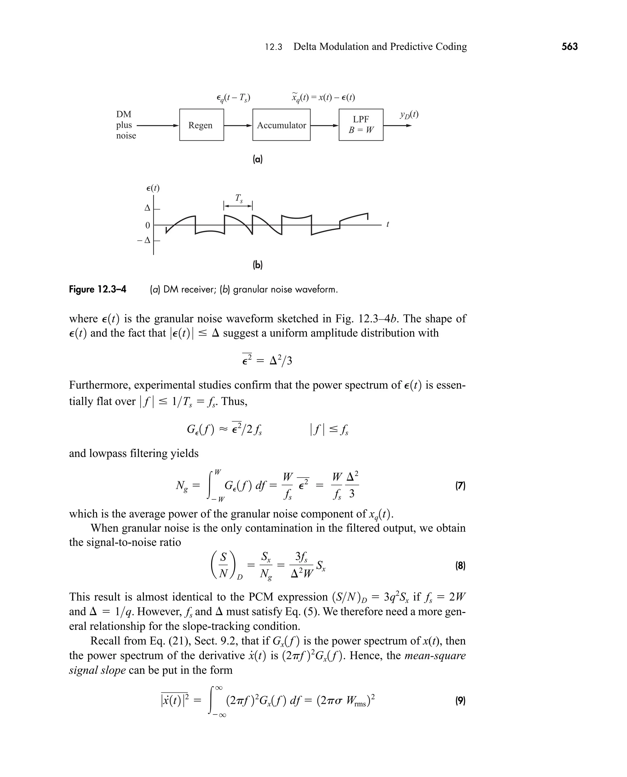
D deviation ratio, or pulse interval
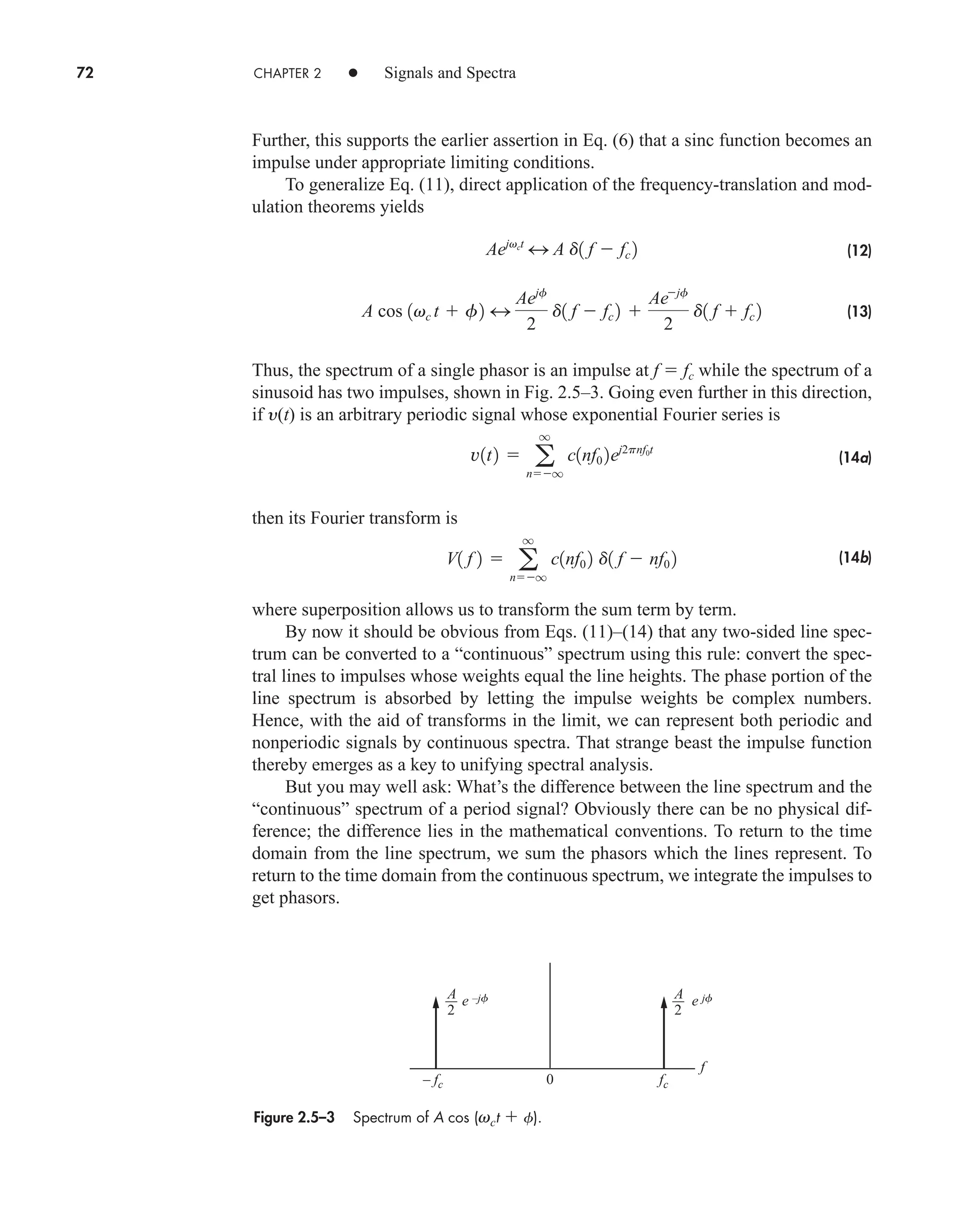
DR dynamic range
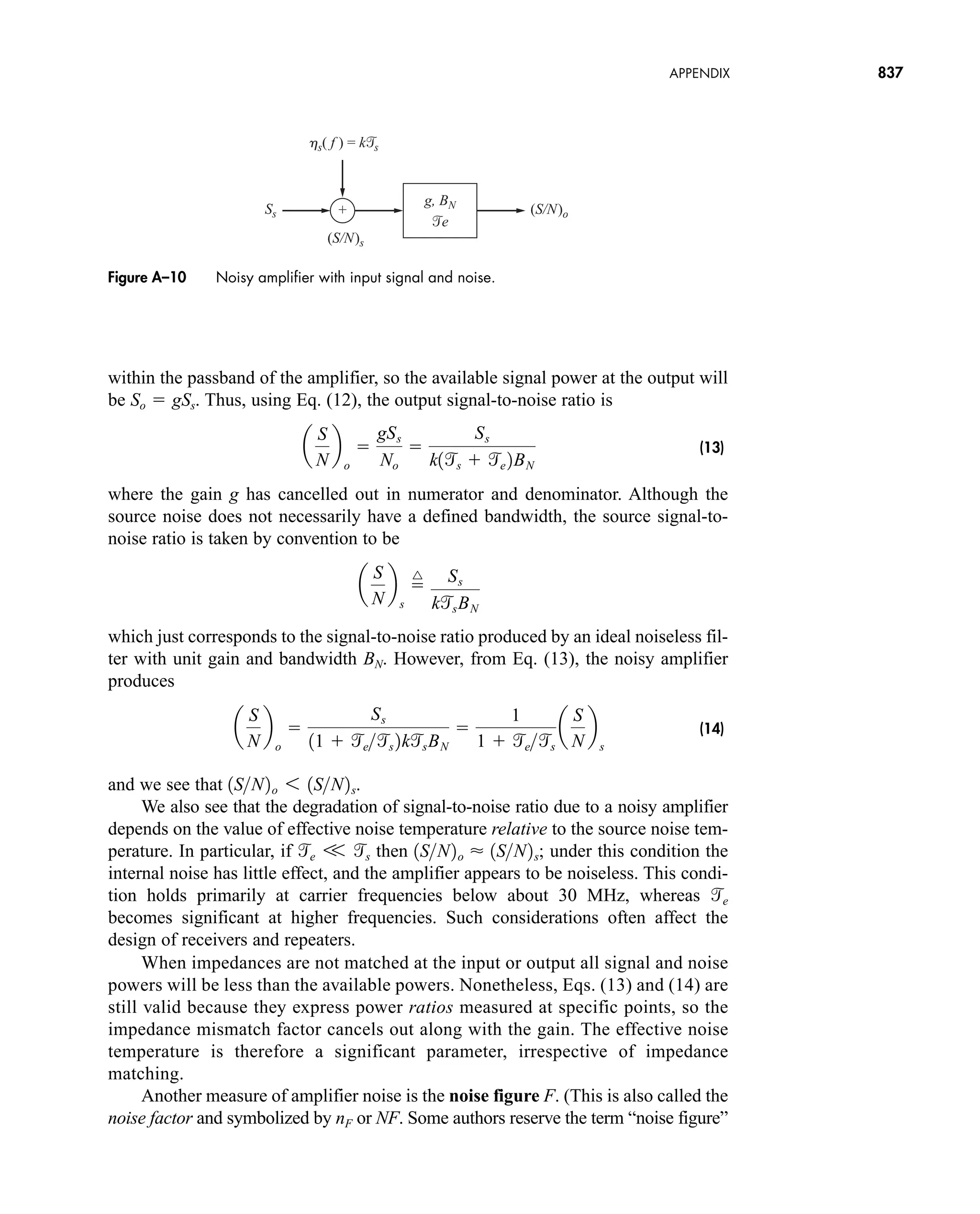
DFT[ ], IDFT[ ] discrete and inverse discrete Fourier transorm
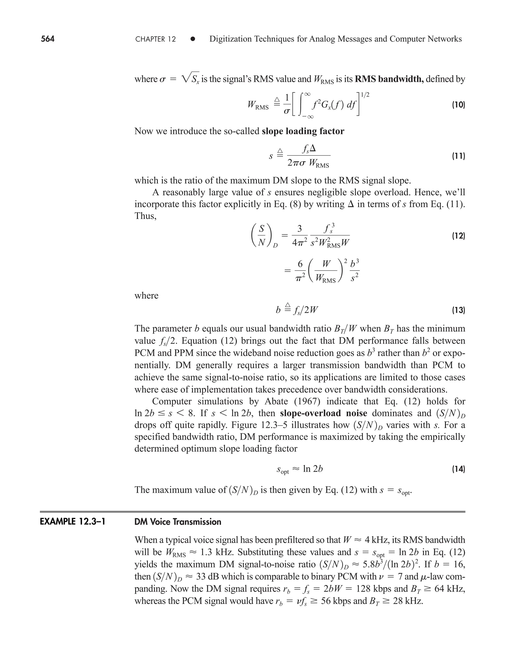
E error vector
E, E1, E0, Eb signal energy, energy in bit 1, energy in bit 0, and bit energy
E[ ] expected value operator
FX(x) cumulative distribution function of X
FXY(x,y) joint cumulative distribution of X and Y
G generator vector
Gx(f) power spectral density of signal x(t)
Gvw(f) cross-spectral density functions of signals v(t), w(t)
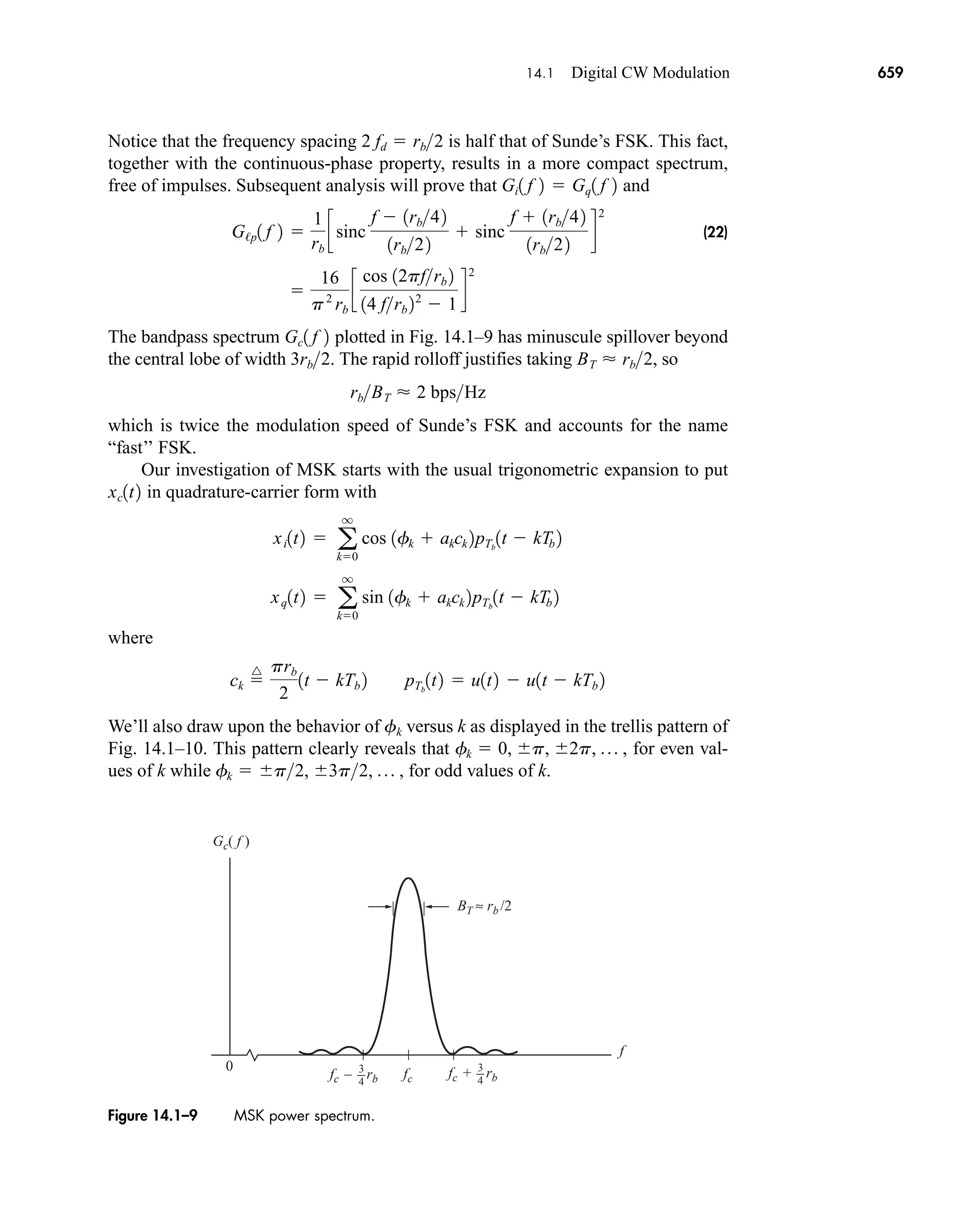
H(f) transfer or frequency-response function of a system
HC(f) channel’s frequency response
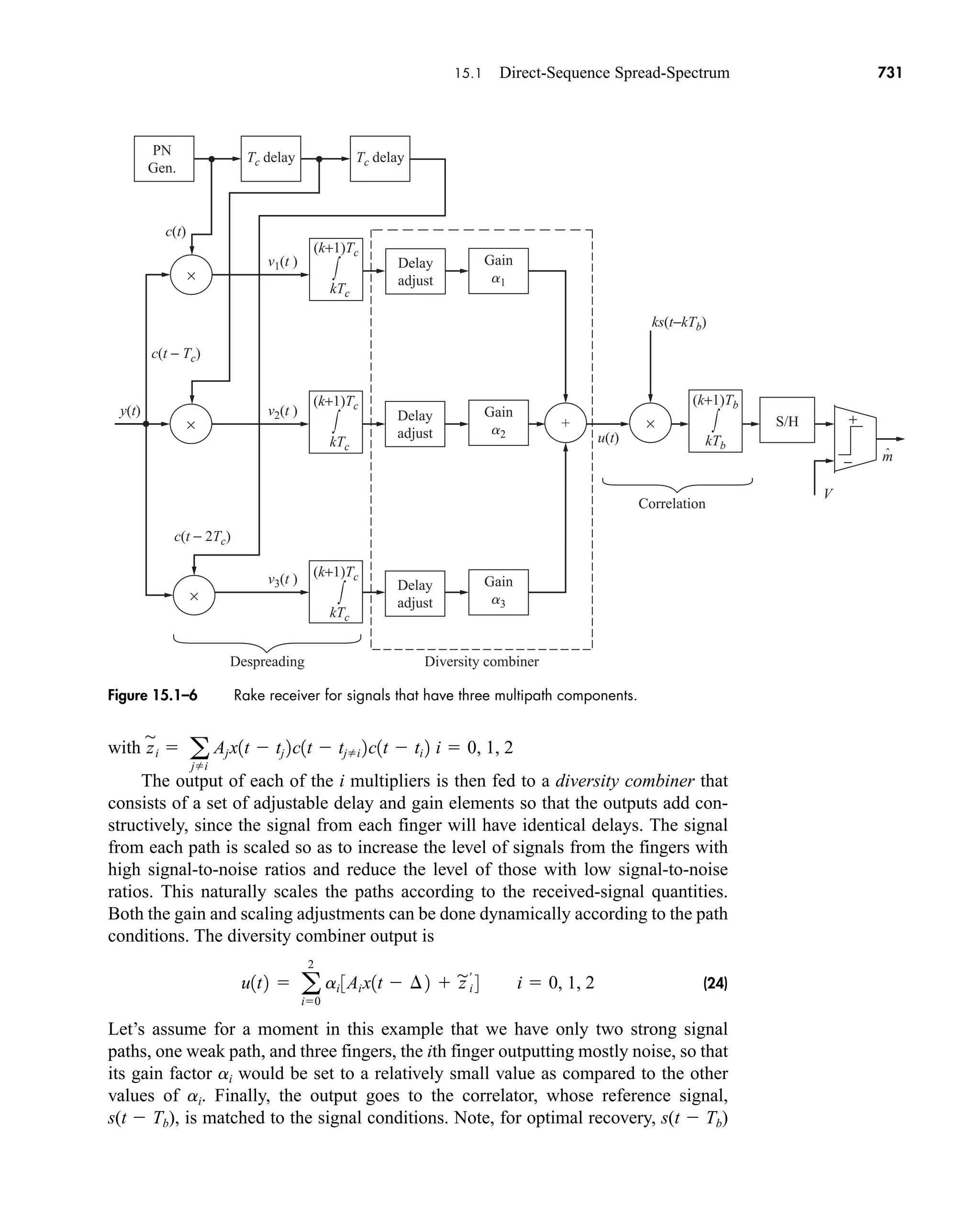
Heq(f) channel equalizer frequency response
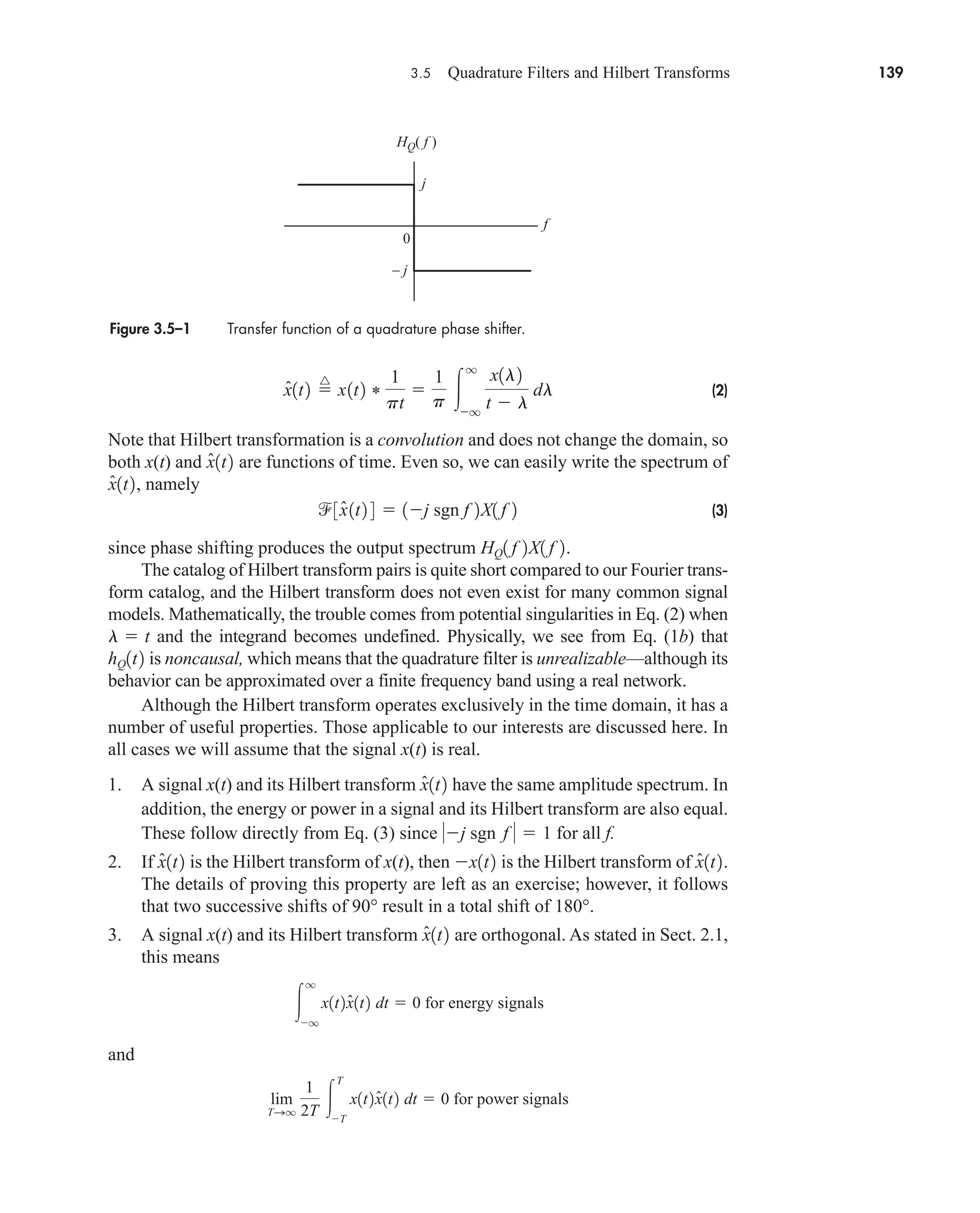
HQ(f) transfer function of quadrature filter
IR image rejection
Jn(b) Bessell function of first kind, order n, argument b
L,LdB loss in linear and decibel units
Lu, Ld uplink and downlink losses
M numerical base, such that q Mv
or message vector
ND destination noise power
NR received noise power
N0 power spectral density or spectral density of white noise
NF, or F noise figure
N(f) noise signal spectrum
P power in watts
Pc unmodulated carrier power
P(f) pulse spectrum
Pe, Pe0, Pe1 probability of error, probability of zero error, probability of 1 error
Pbe, Pwe probability of bit and word errors
Pout, Pin output and input power (watts)
PdBW, PdBmW power in decibel watts and milliwatts
Psb power per sideband
P(A), P(i,n) probability of event A occurring and probability of i errors in n-bit word
Q[ ] gaussian probability function
car80407_fm_i-xx.qxd 9/1/09 8:59 AM Page xvii](https://image.slidesharecdn.com/communicationsystemsanintro-a-241115060943-61721fa8/75/Communication_Systems__An_Intro_-_A-_Bruce_Carlson_-pdf-19-2048.jpg)

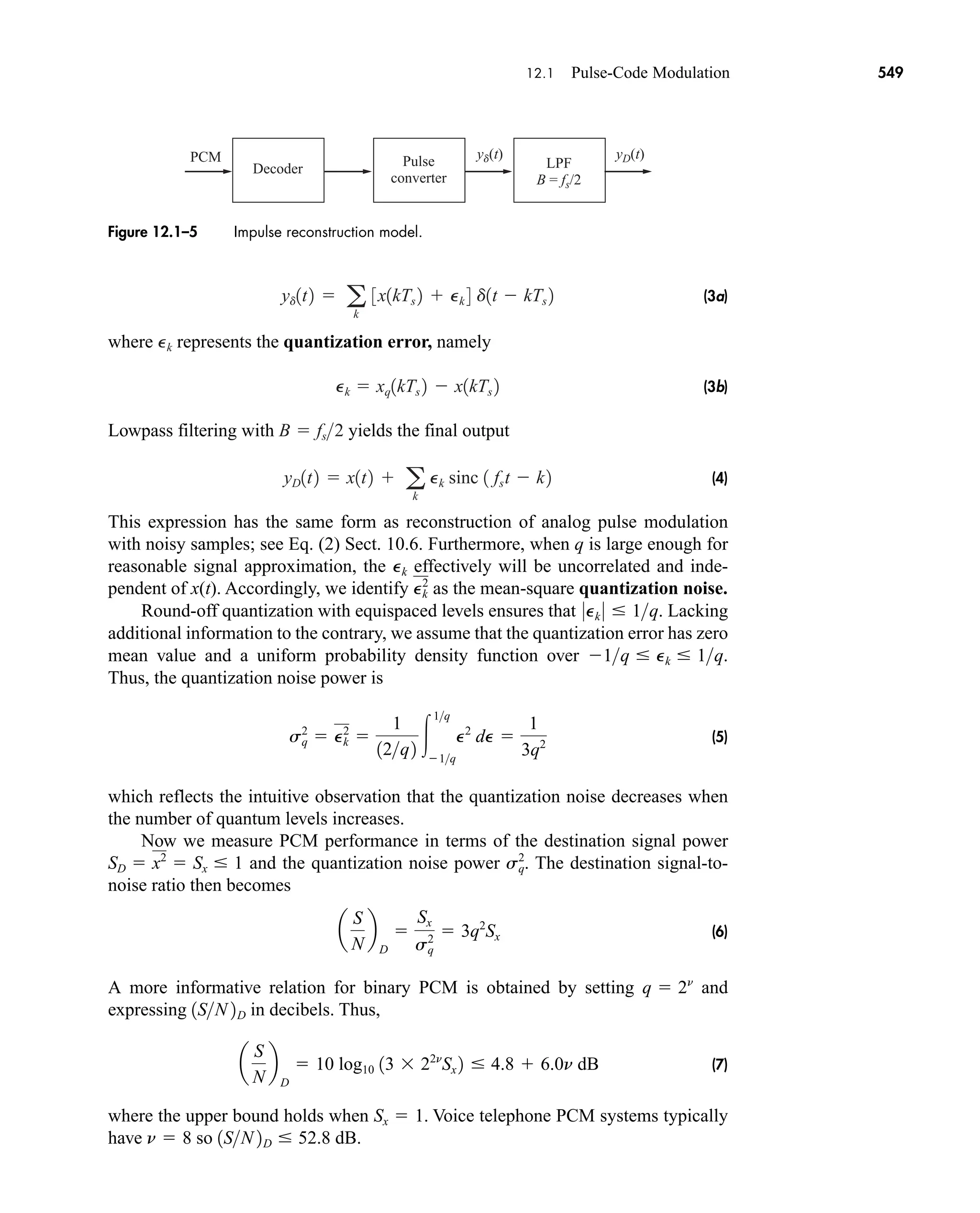
![Mathematical Symbols xix
Mathematical Symbols xix
h(t) impulse-response function of a system
hC(t) impulse-response function of a channel
hk(t), hk(n) impulse-response function of kth portion of subchannel
hQ(t) impulse-response function of a quadrature filter
Im[x] and Re[x] imaginary and real components of x
j imaginary number operator
l length in kilometers
m number of repeater sections
mk, k actual and estimated k message symbol
n(t) noise signal
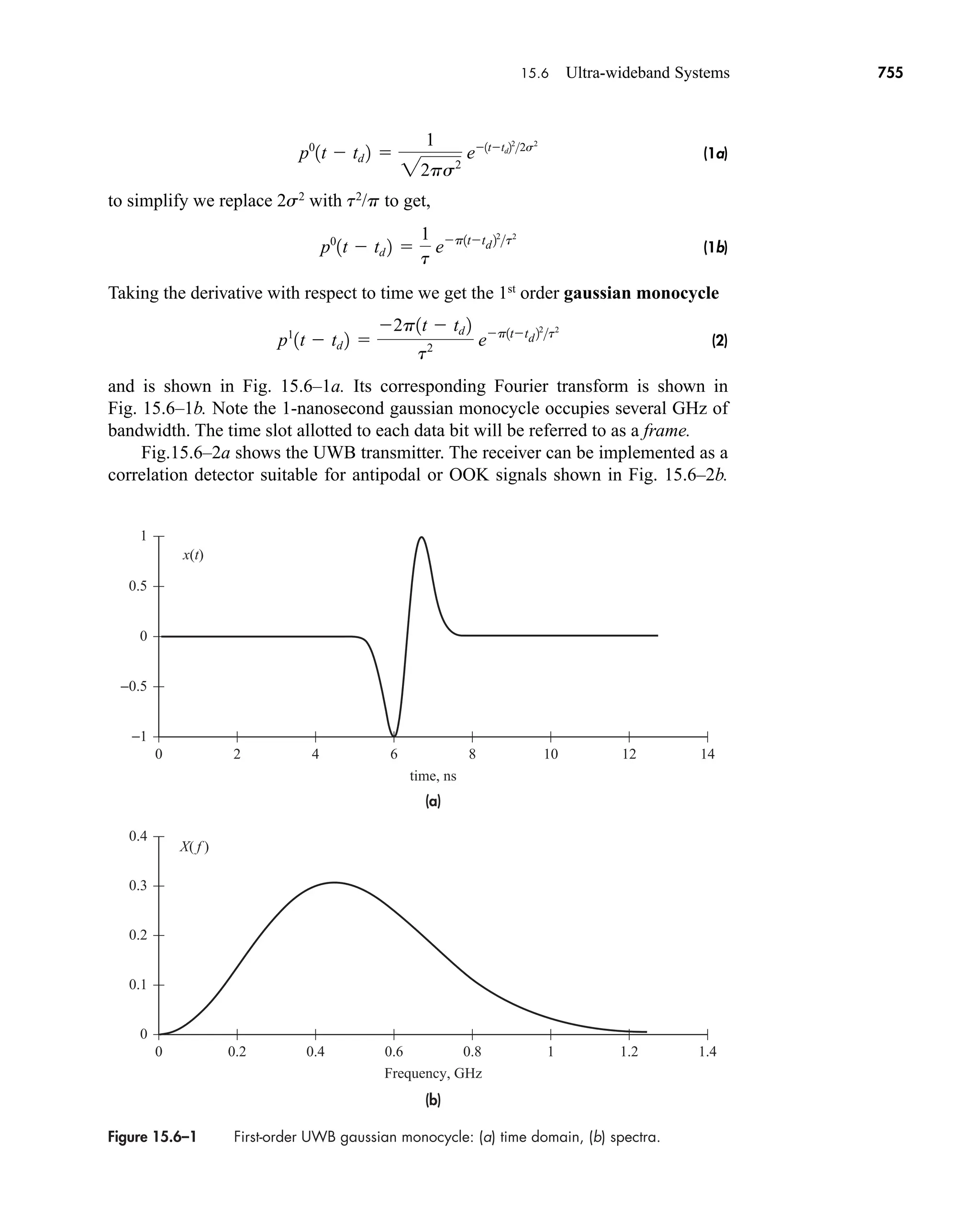
p(t) pulse signal
p0
(t), p1
(t) gaussian and first-order monocycle pulses
output of transversal filter’s nth delay element
input to equalizing filter
peq(tk) output of an equalizing filter
pX(x) probability density function of X
pXY(x) joint probability density function of X and Y
q number of quantum levels
r, rb signal rate, bit rate
s(t) switching function for sampling
s0(t), s1(t) inputs to multiplier of correlation detector
sgn(t) signum function
t time in seconds
td time delay in seconds
tk kth instant of time
tr rise time in seconds
u(t) unit step function, or output from rake diversity combiner
v number of bits
v(t) input to a detector
vk (t) kth subcarrier function
v(t) average value of v(t)
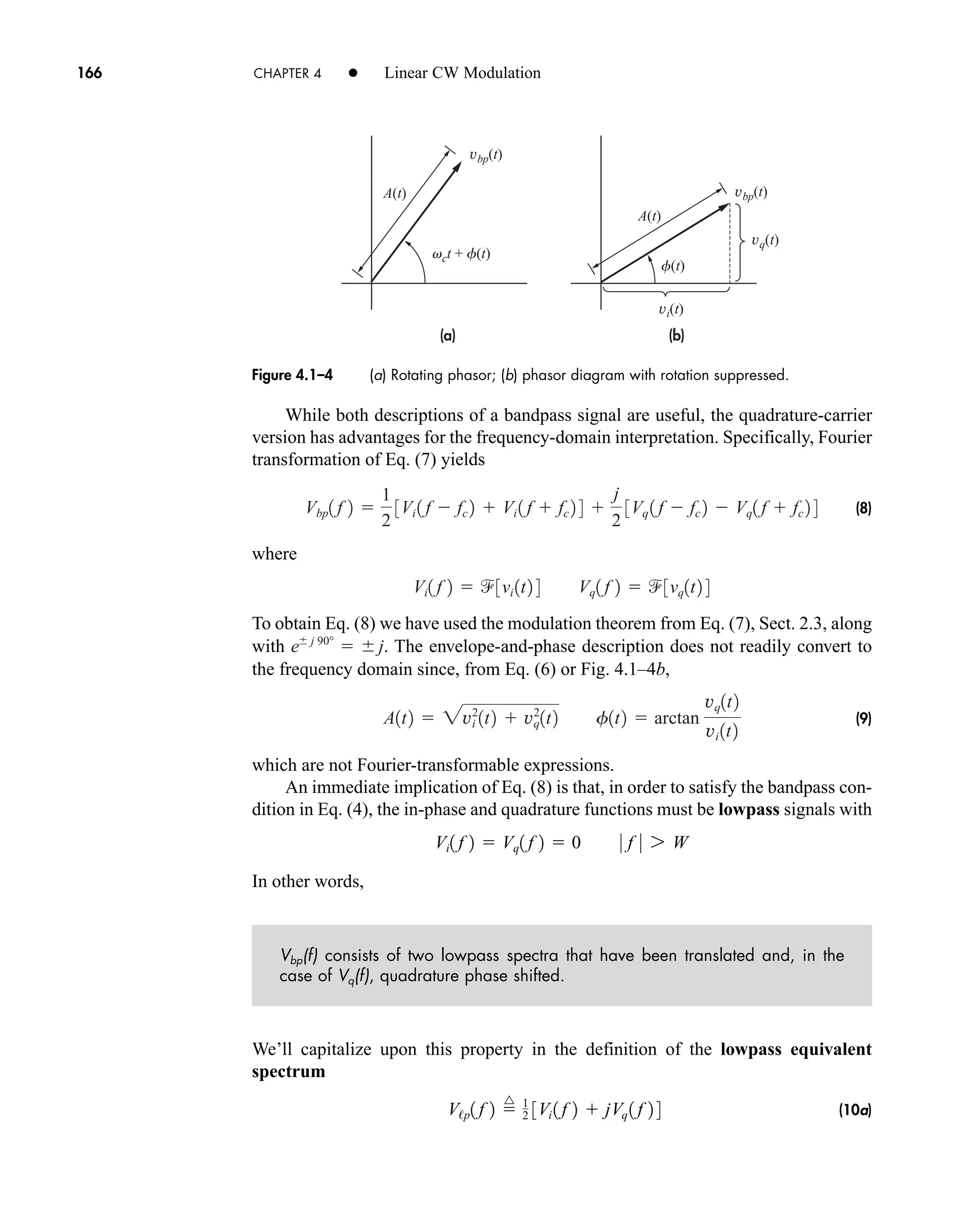
vbp(t) time-domain expression of a bandpass signal
w*(t) complex conjugate of w(t)
Hilbert transform of x, or estimate of x
x(t), y(t) input and output time functions
x(t) message signal
x(k), x(kTs) sampled version of x(t)
X(n) discrete Fourier transform of x(k)
xb(t) modulated signal at a subcarrier frequency
xc(t) modulated signal
xq(k) quantized value for kth value of x
y(t) detector output
xk(t), yk(t) subchannel signal
yD(t) signal at destination
zm(t) output of matched filter or correlation detector
x̂
p
1t2
p
n
m̂
car80407_fm_i-xx.qxd 9/1/09 8:59 AM Page xix](https://image.slidesharecdn.com/communicationsystemsanintro-a-241115060943-61721fa8/75/Communication_Systems__An_Intro_-_A-_Bruce_Carlson_-pdf-21-2048.jpg)

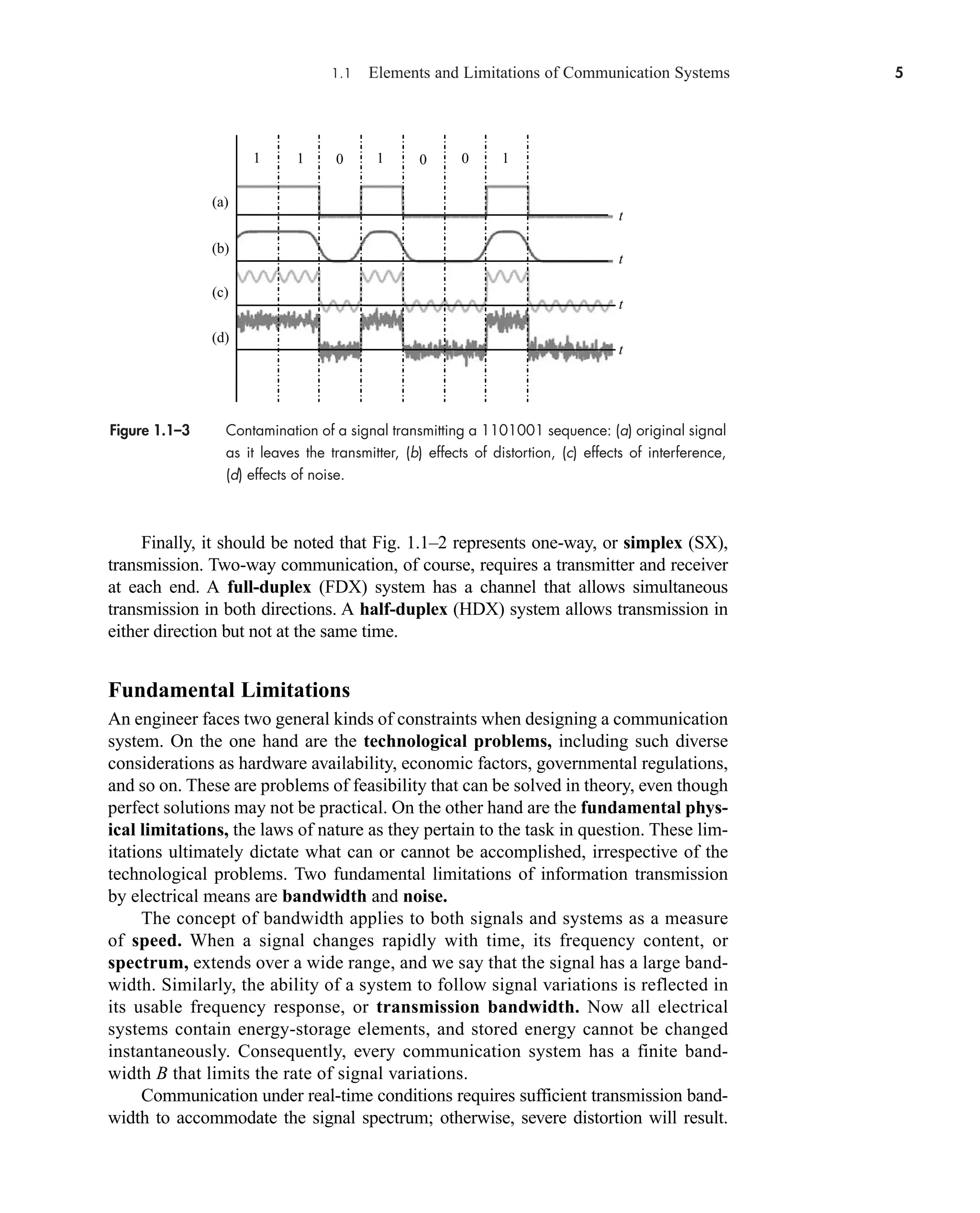

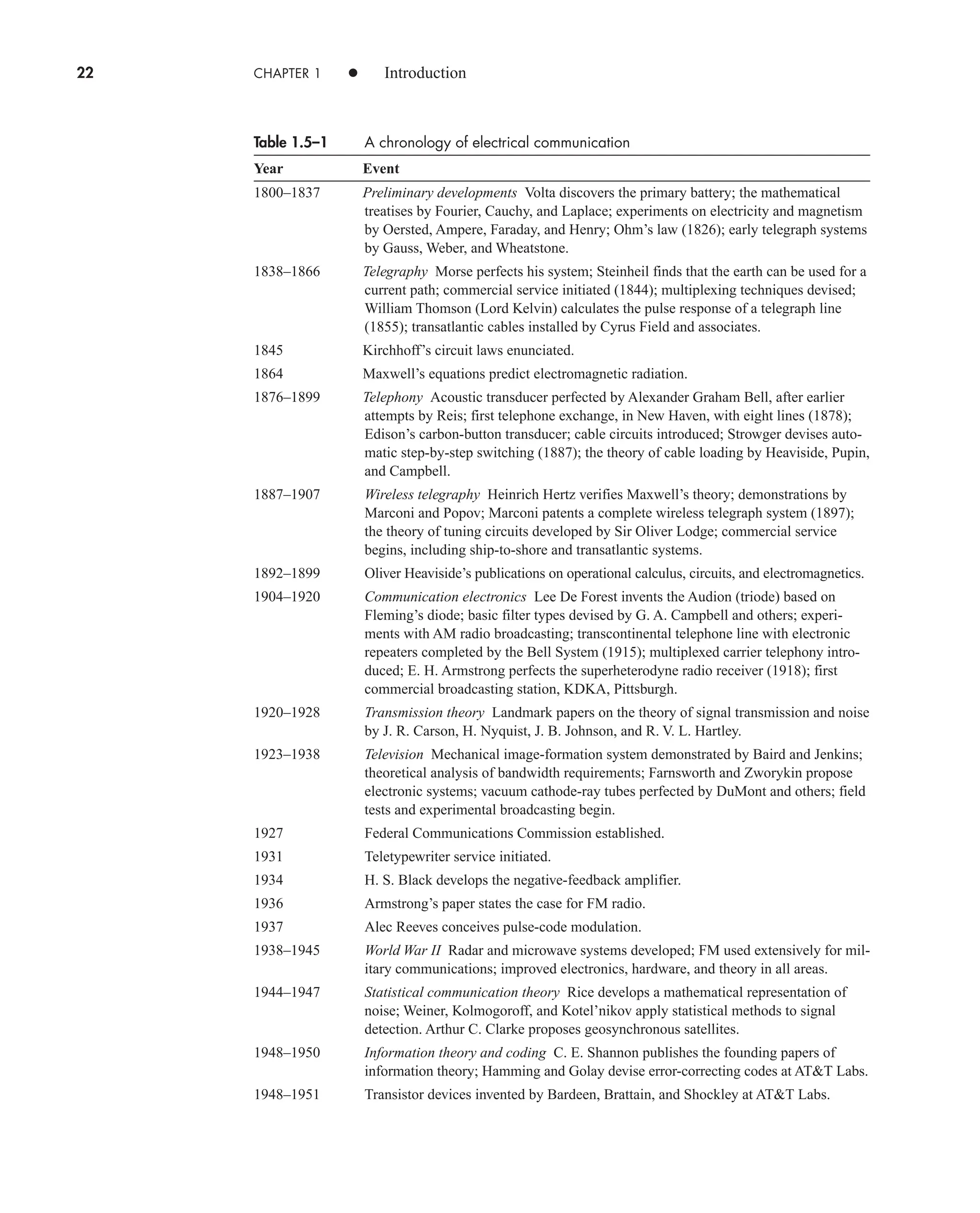
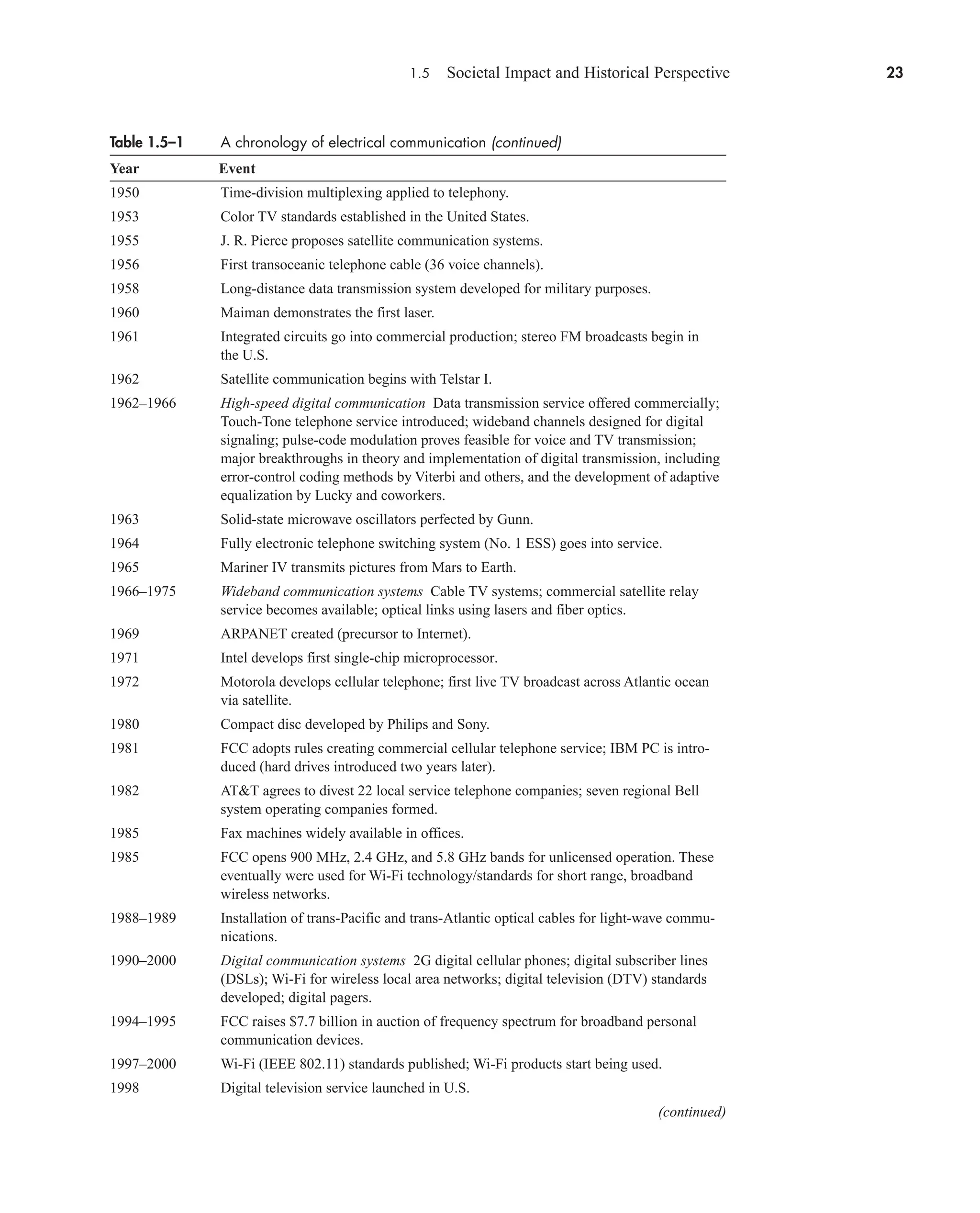
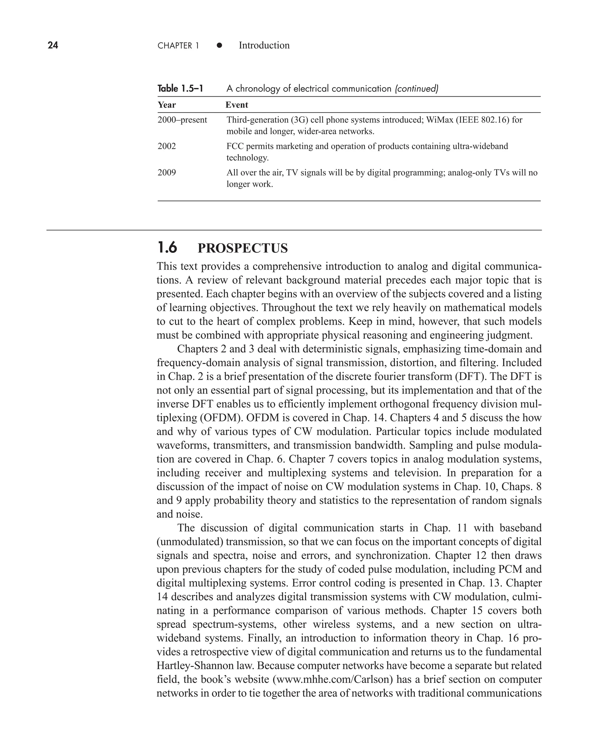

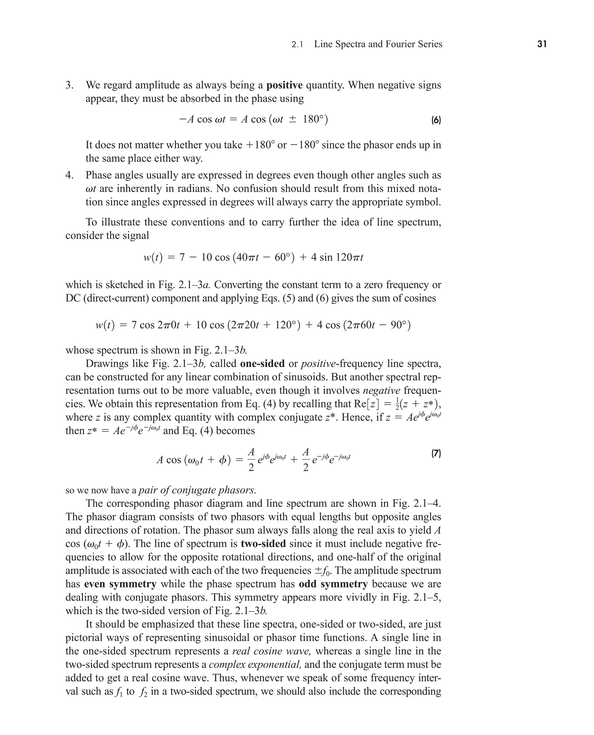
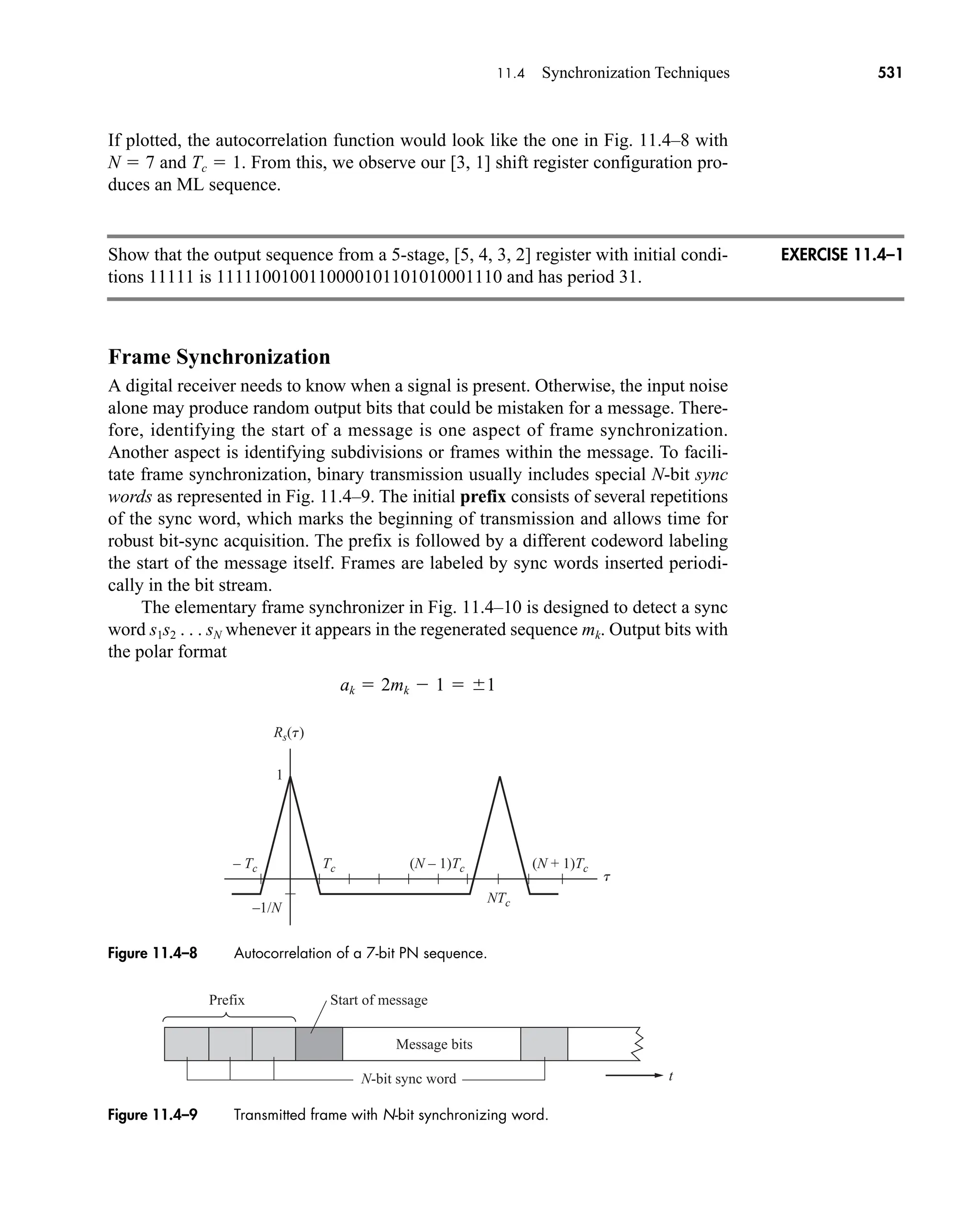
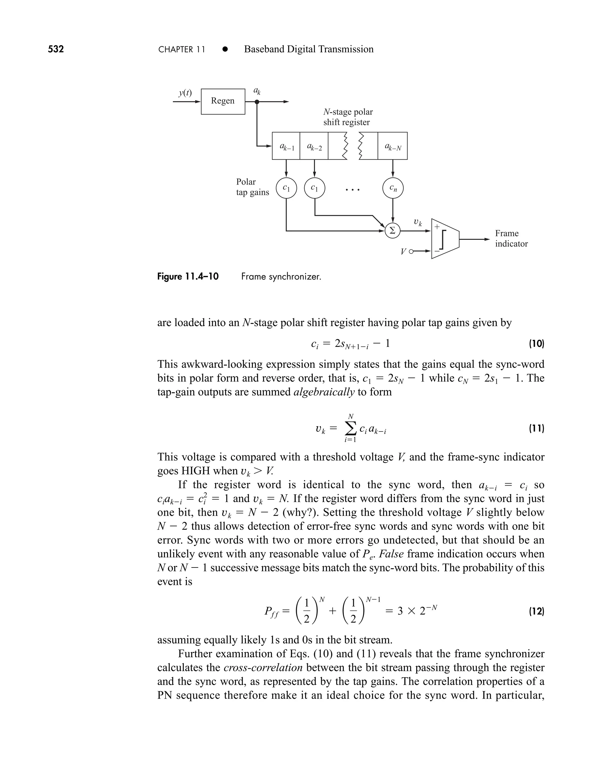
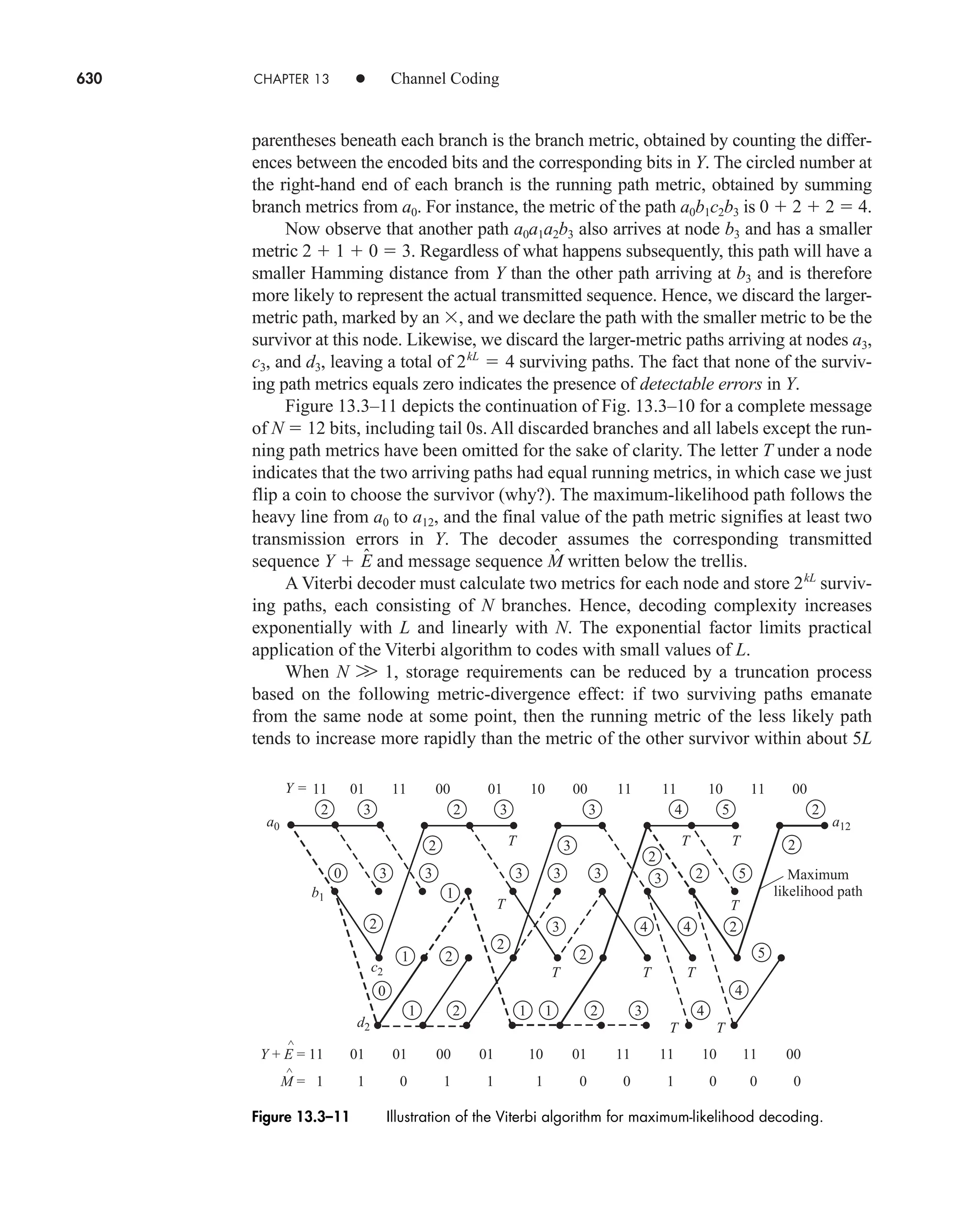
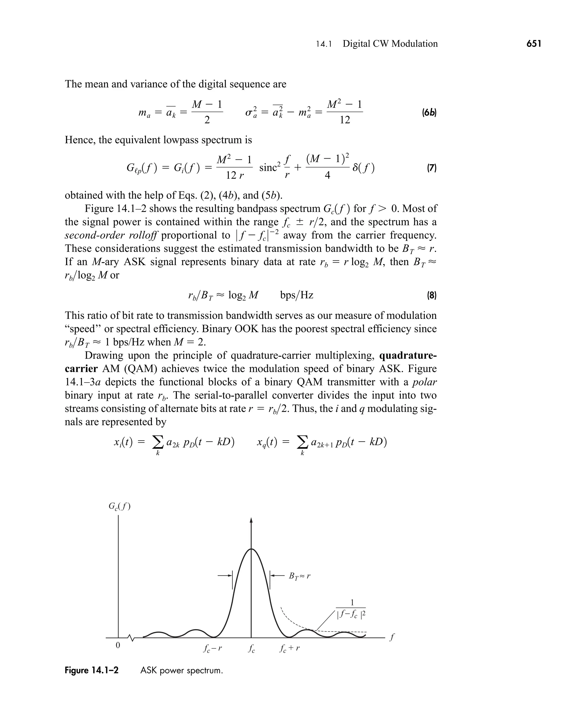
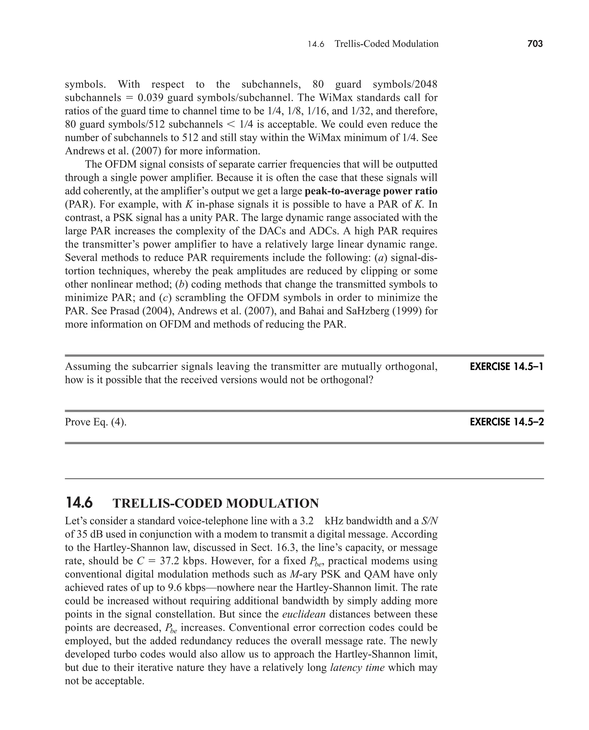
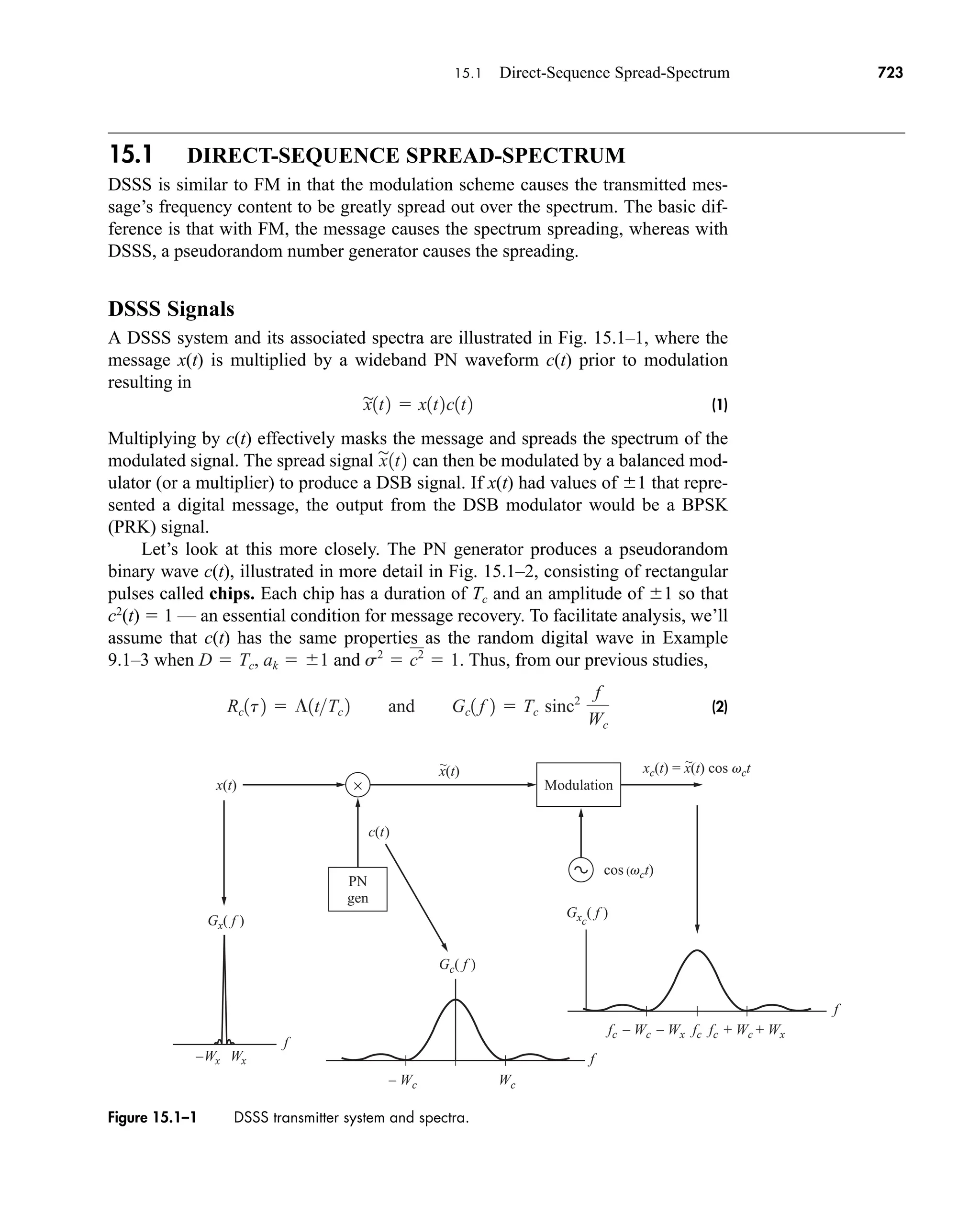
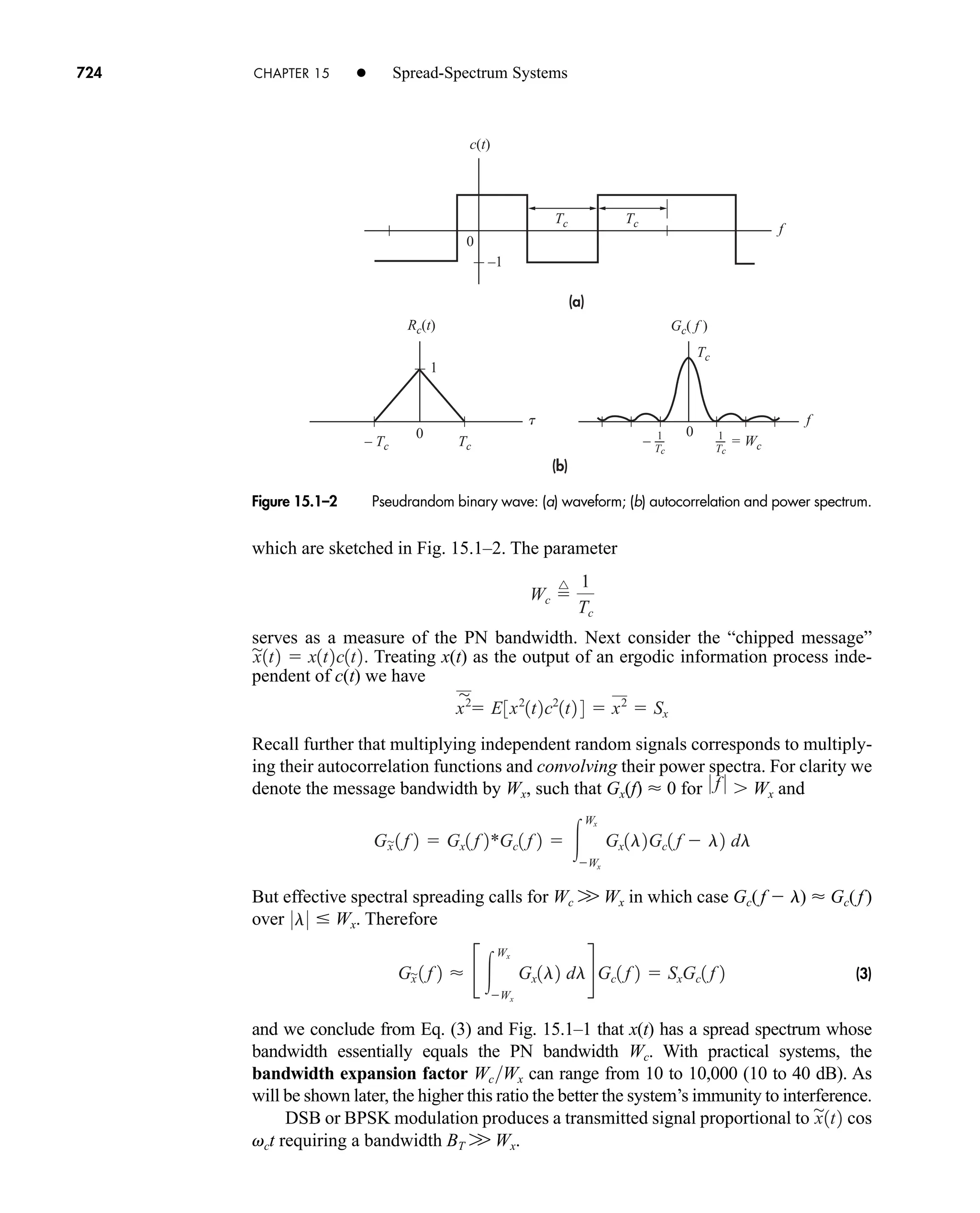
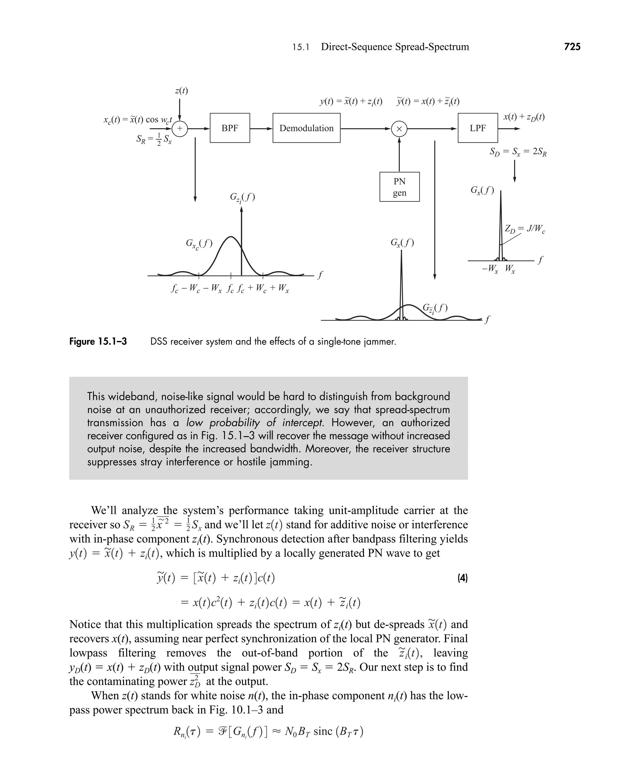
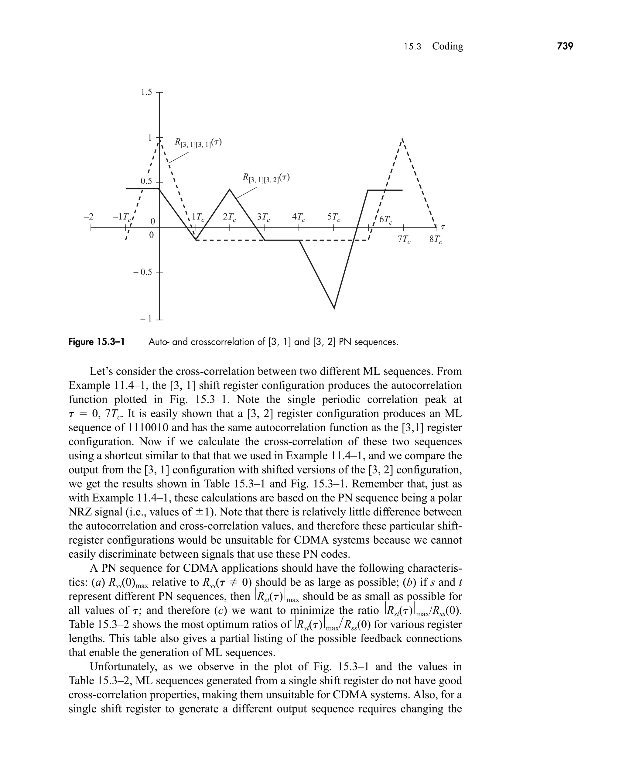
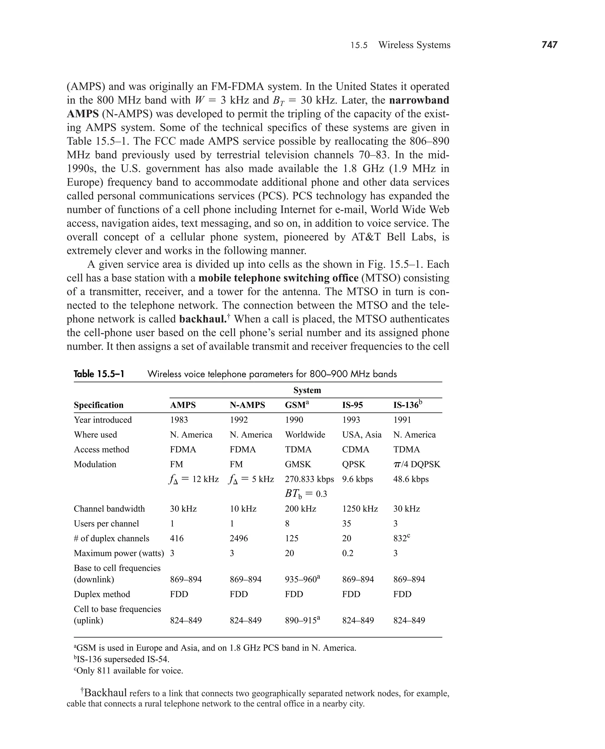
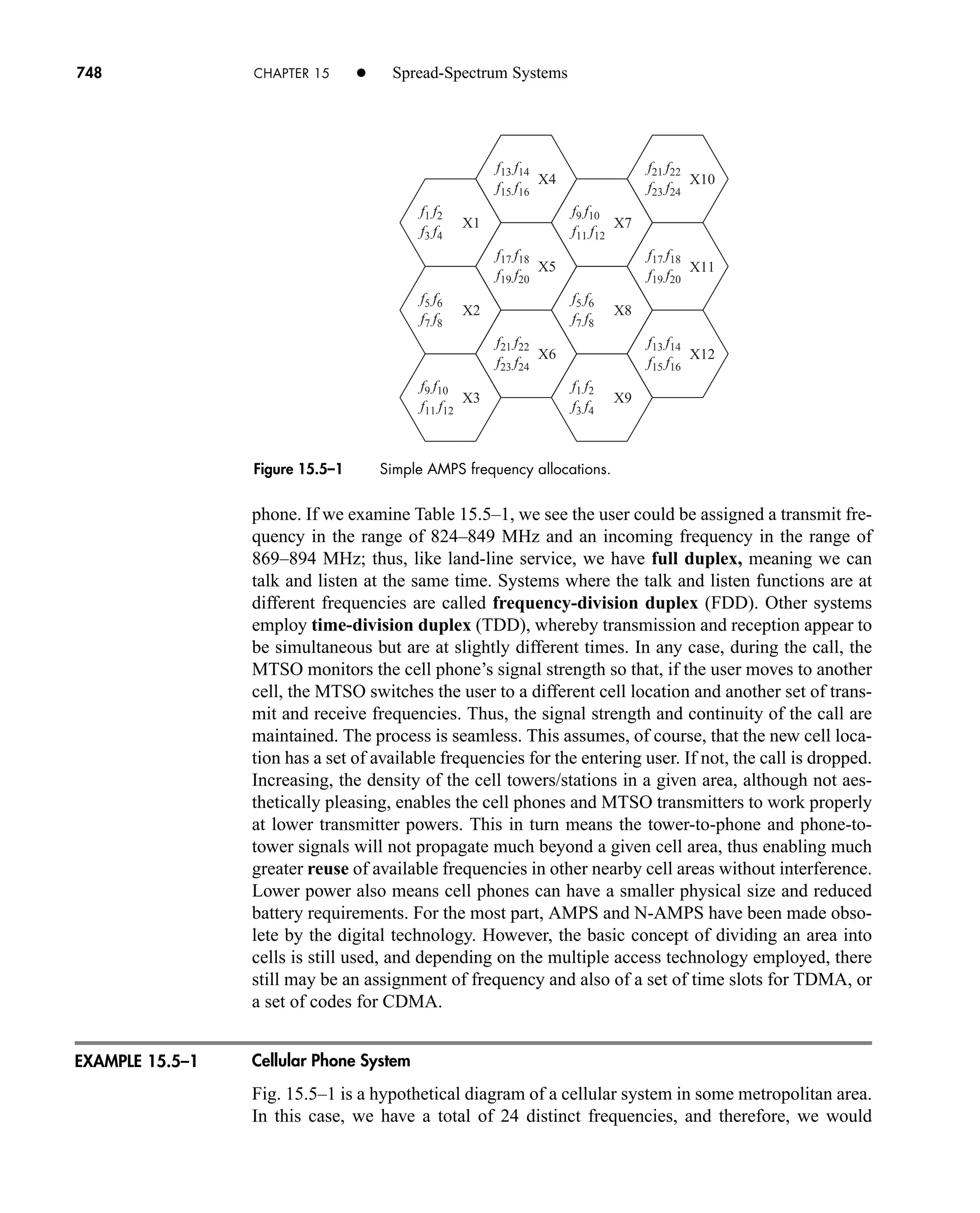
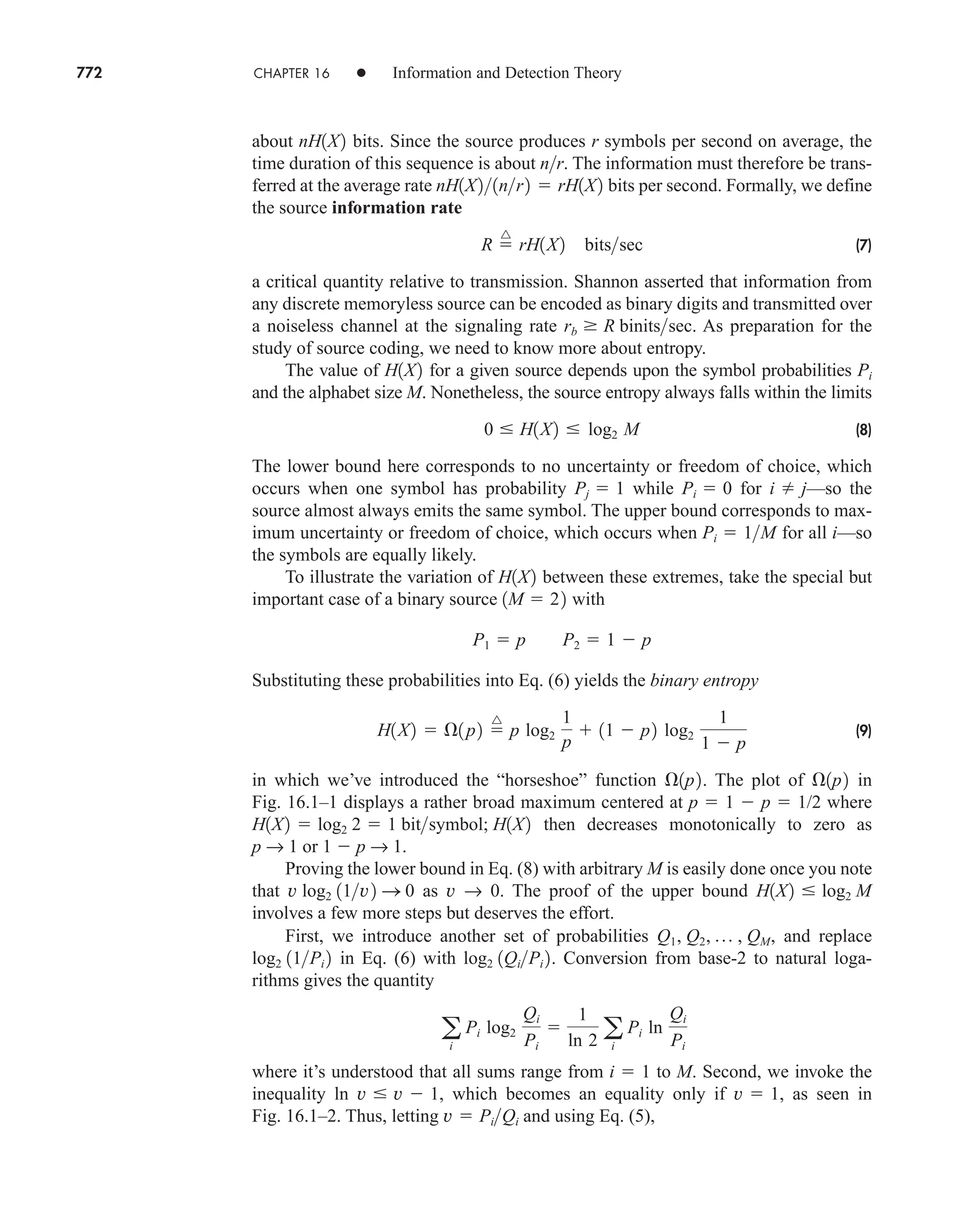
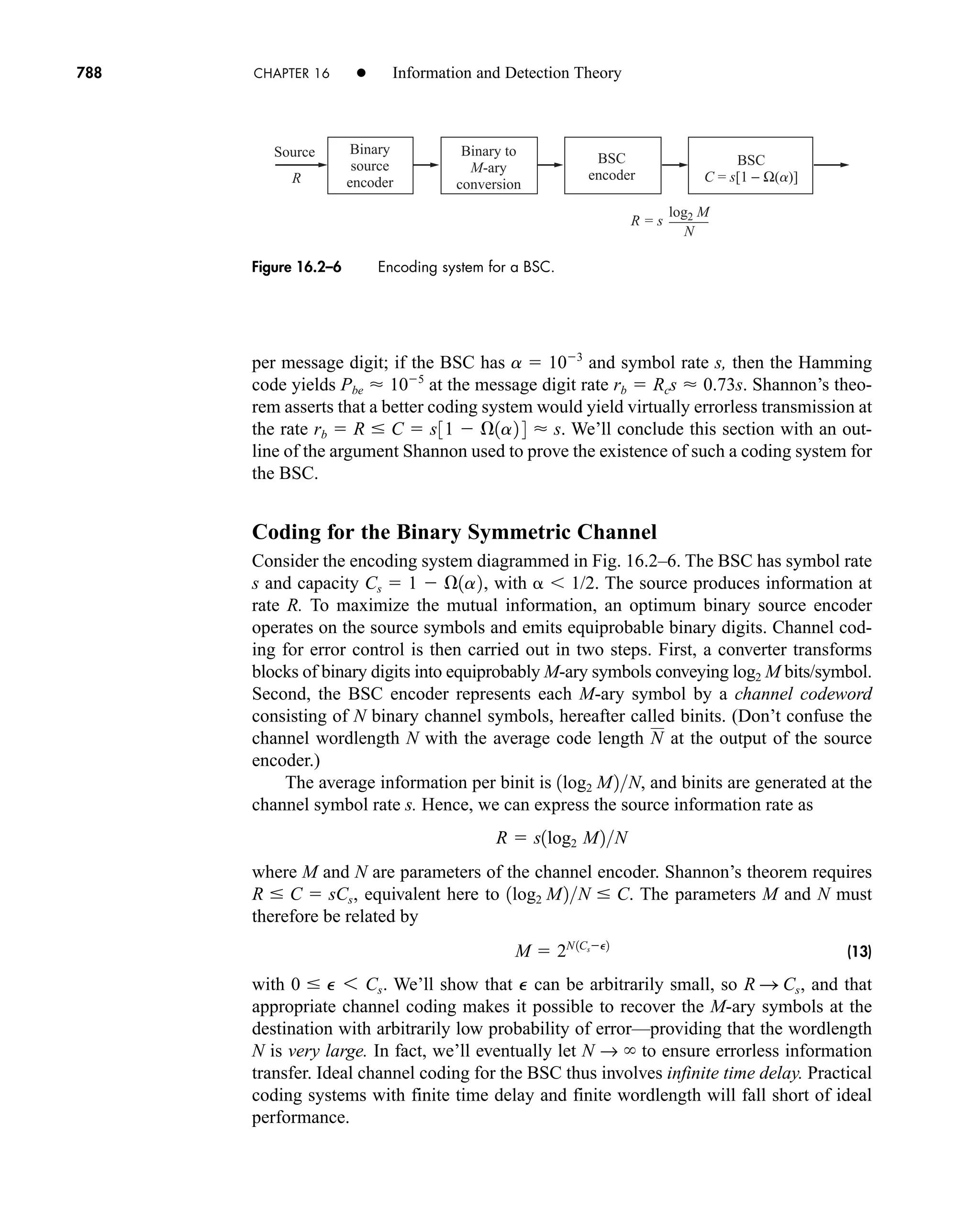
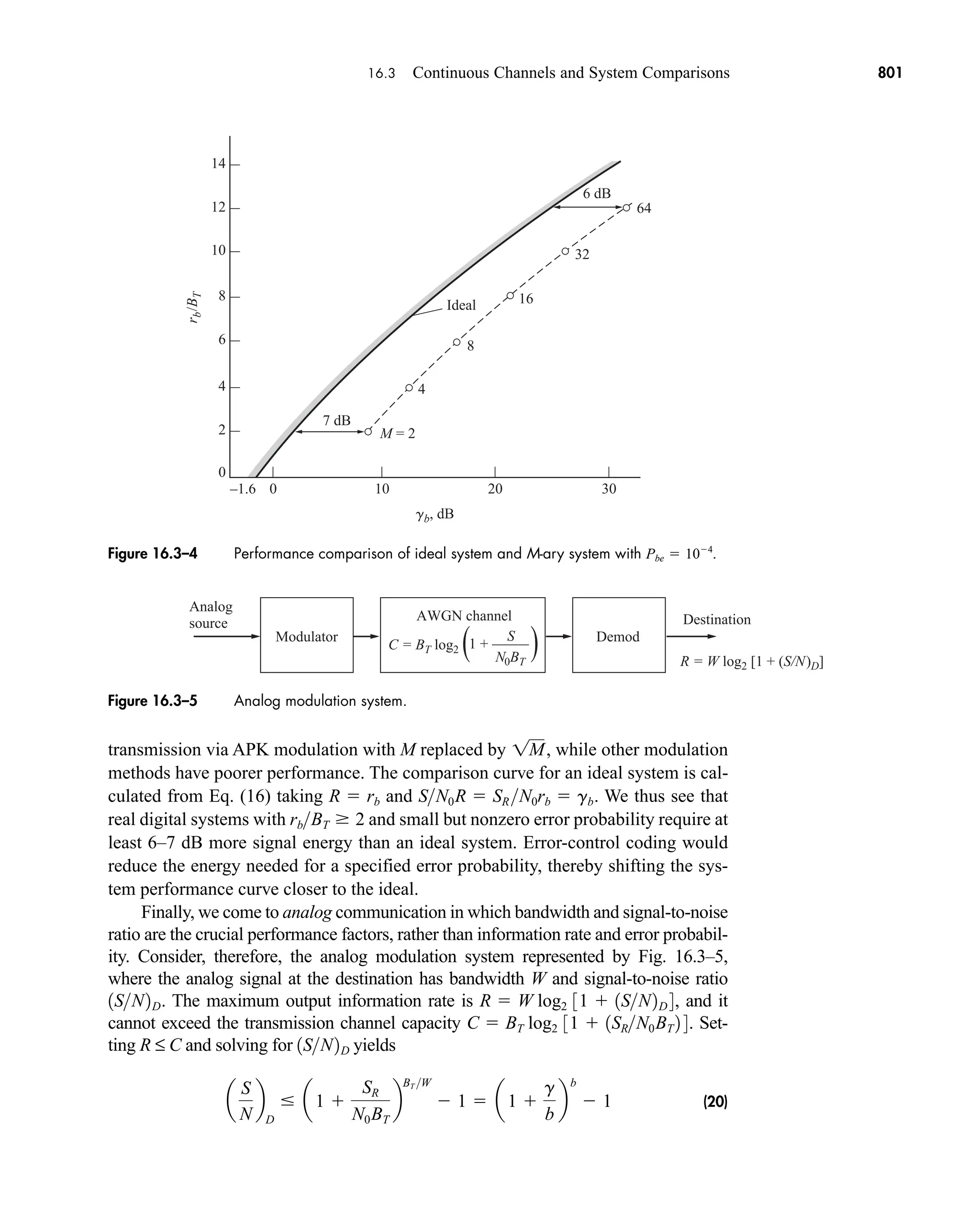
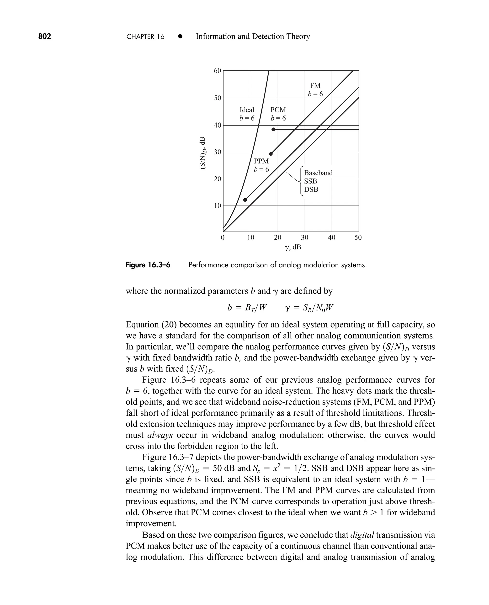
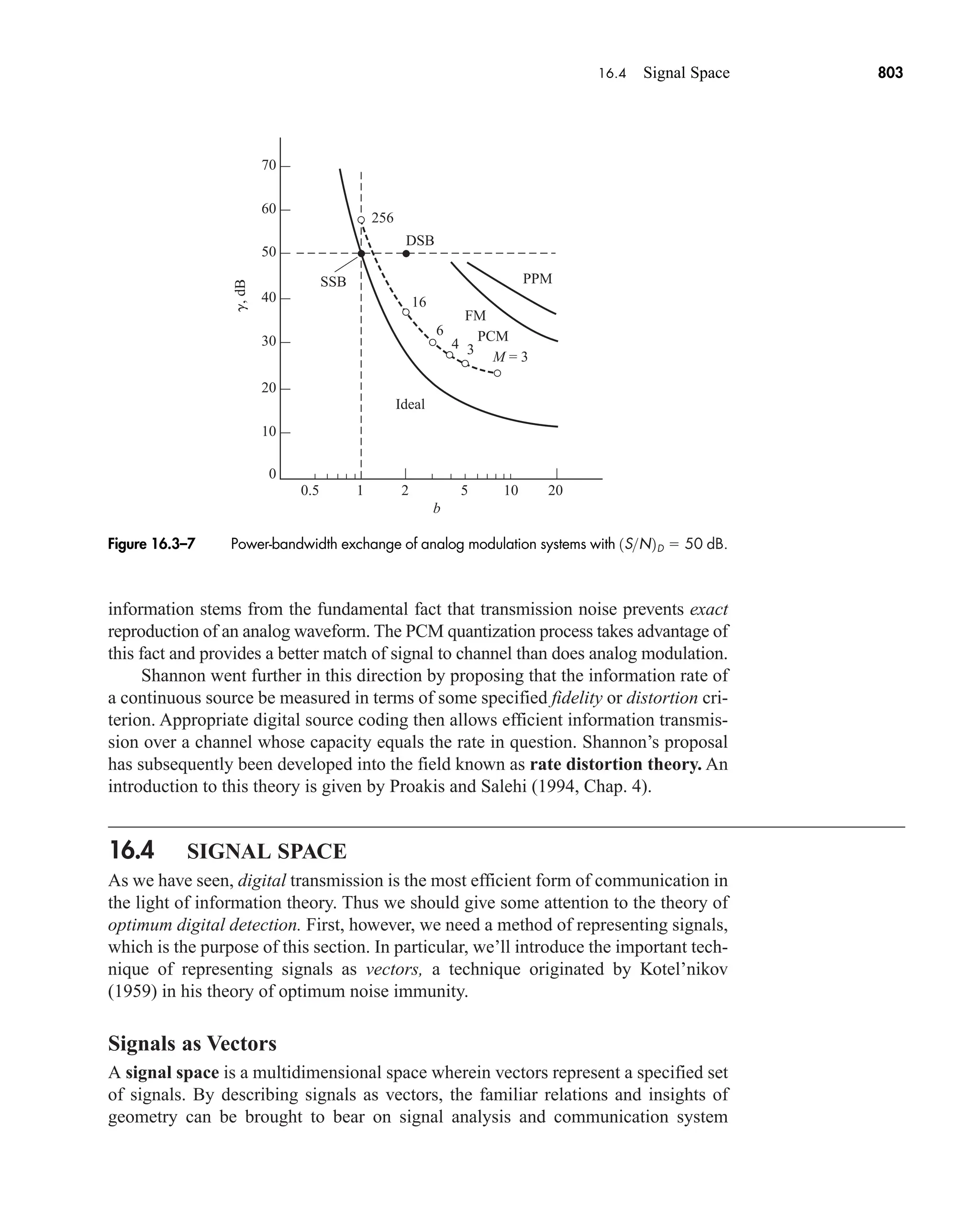
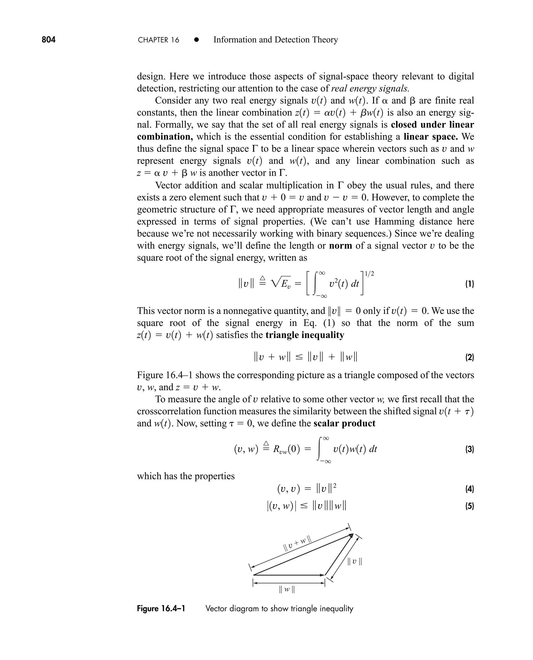
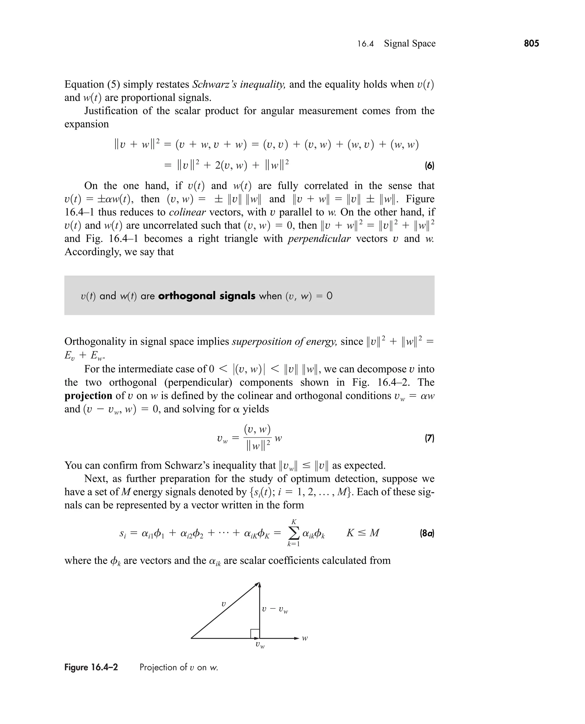
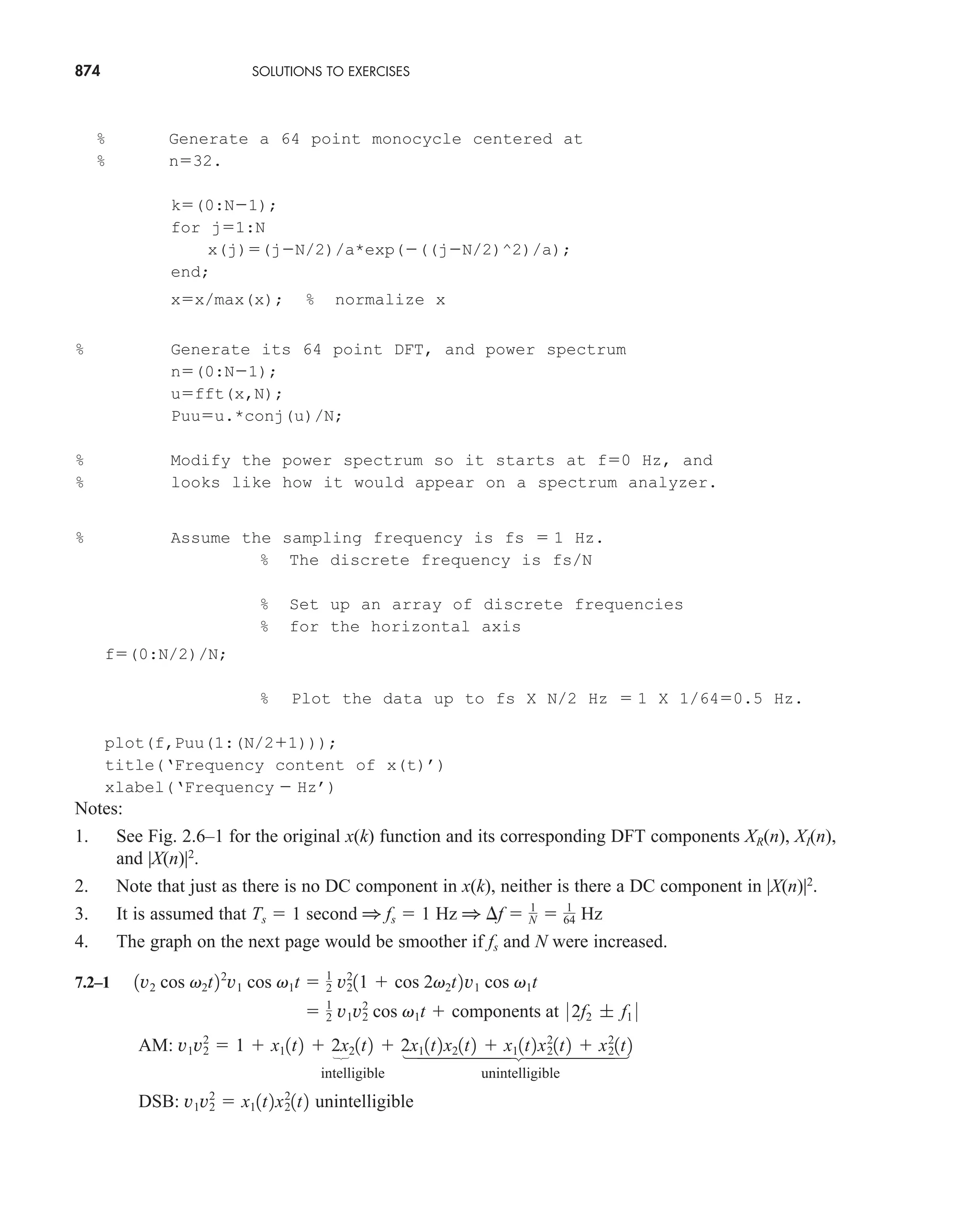
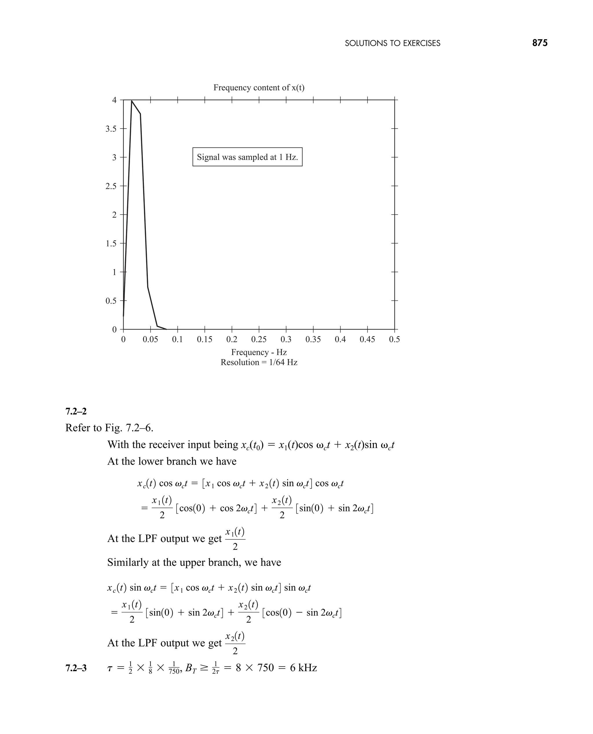
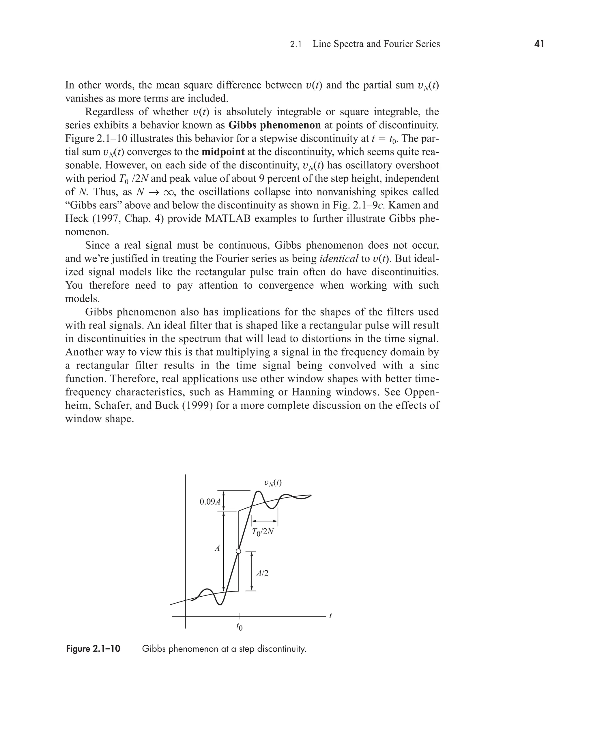
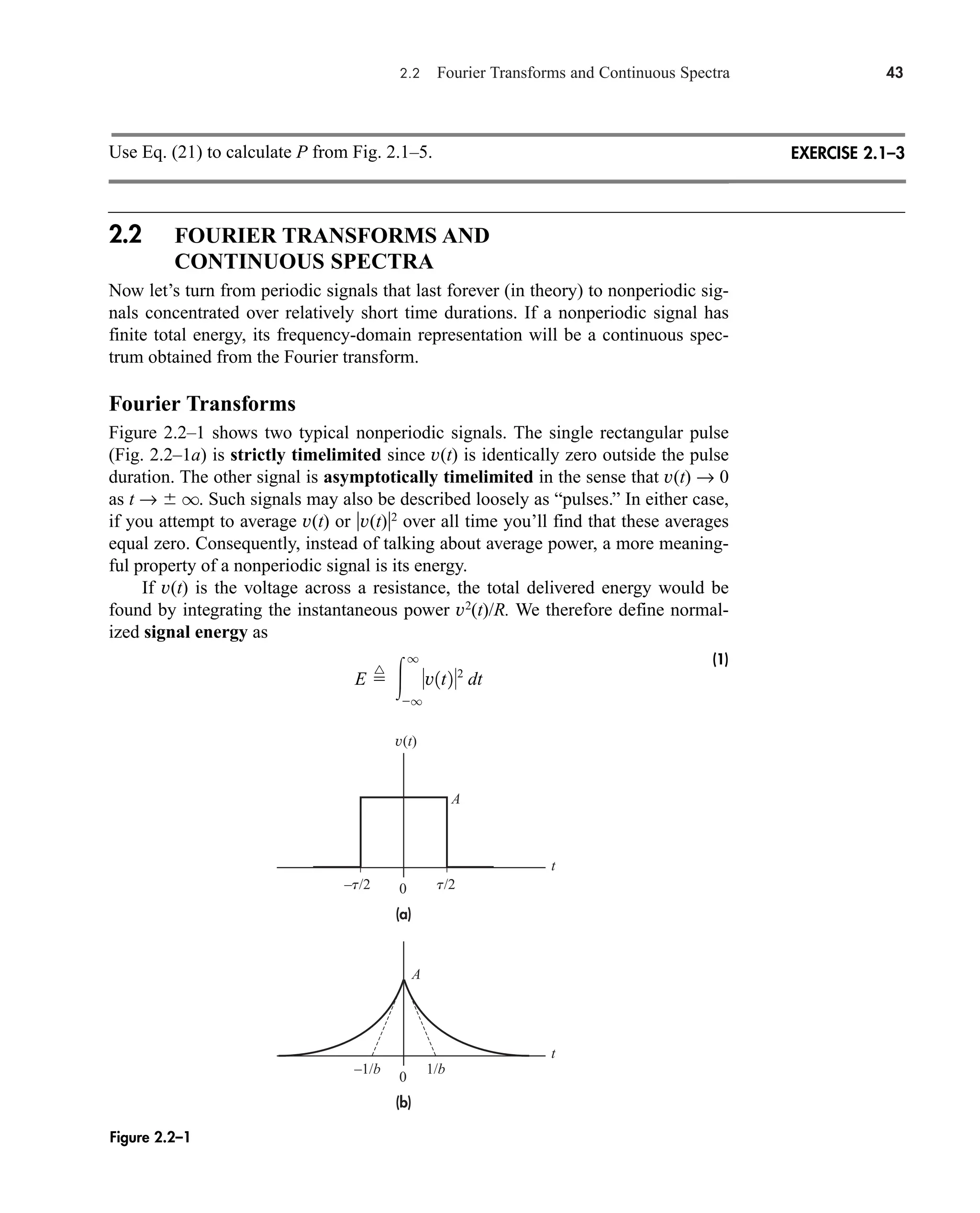
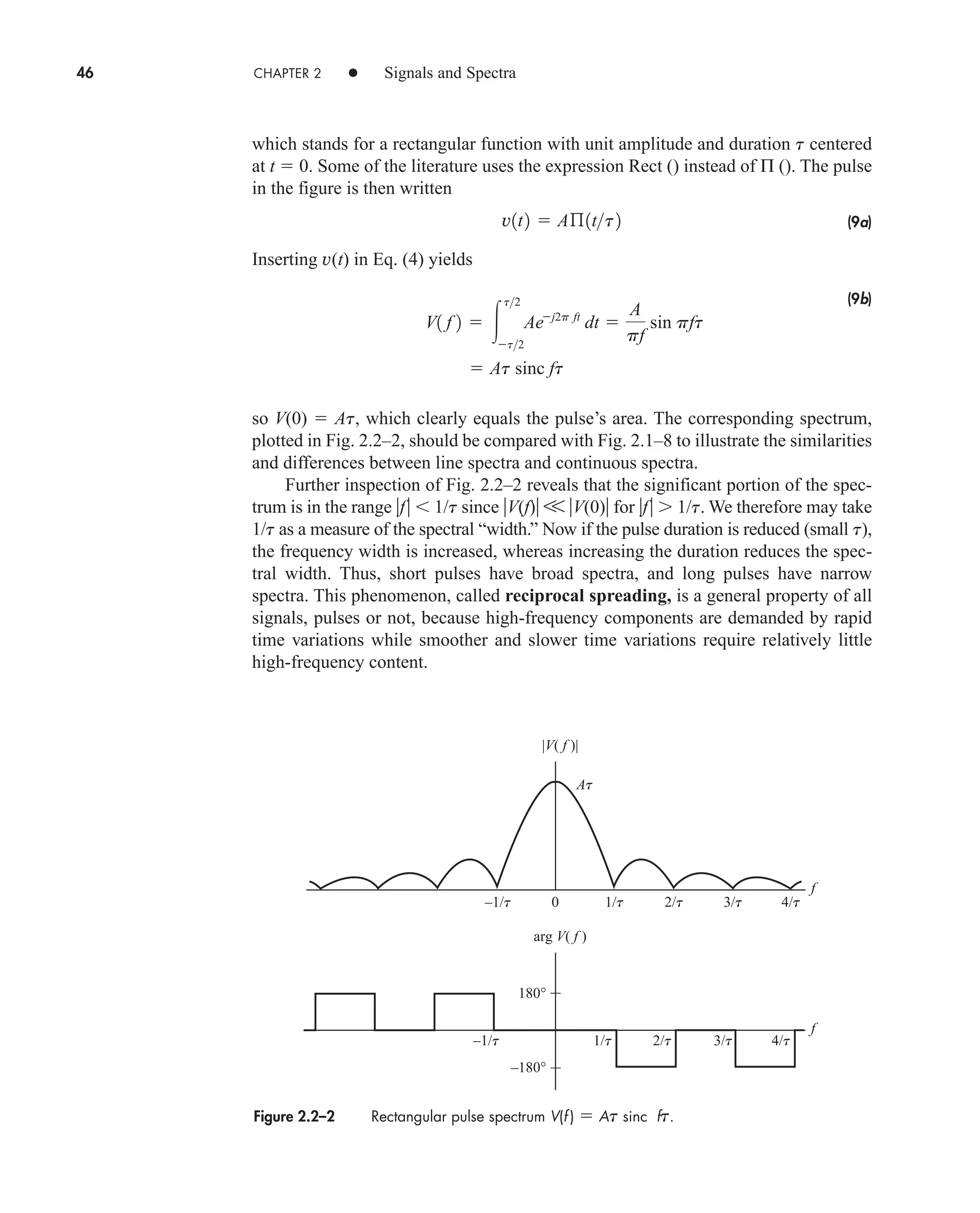
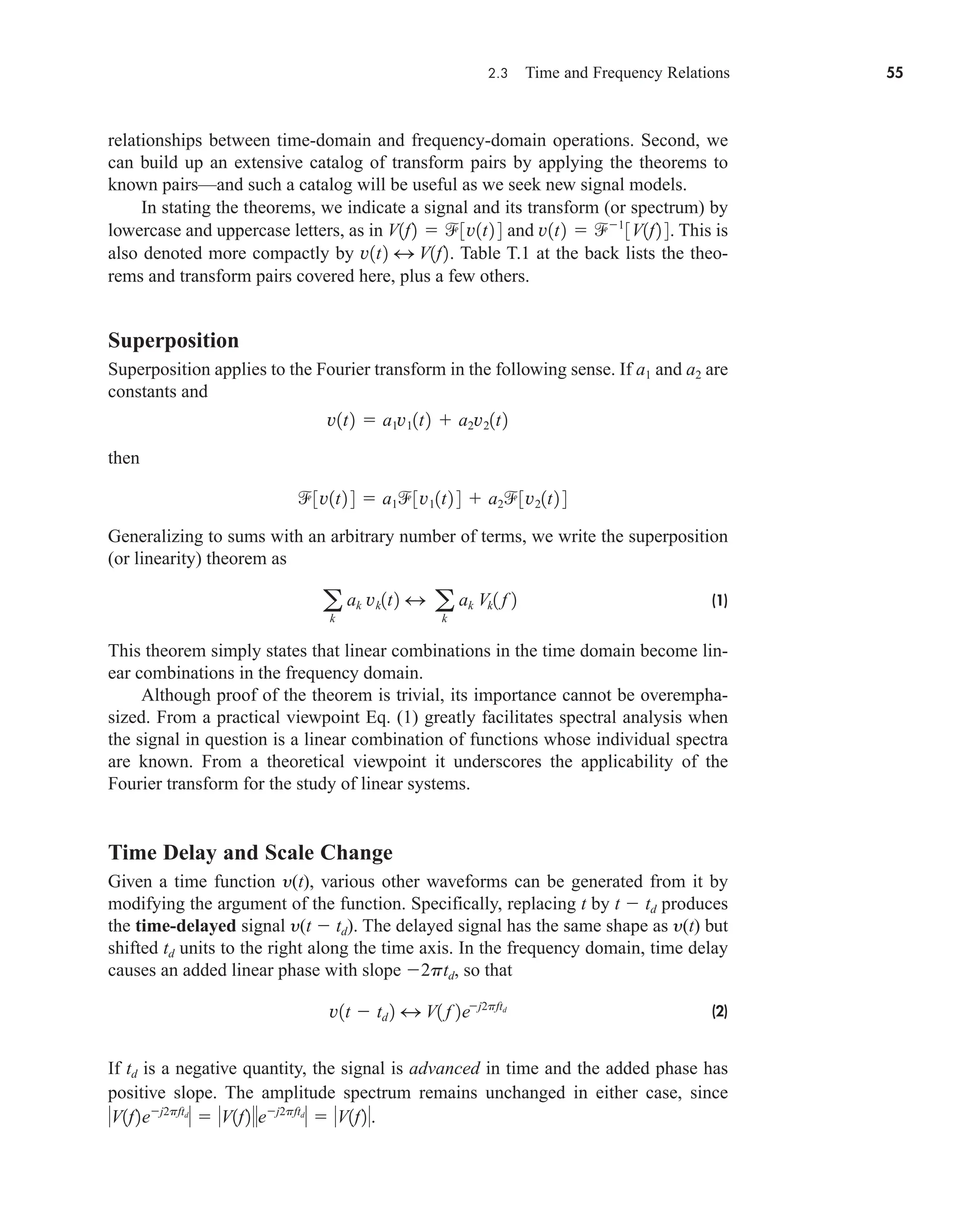
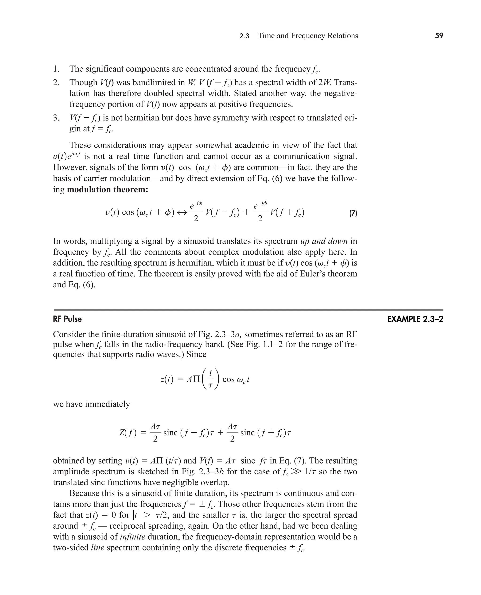
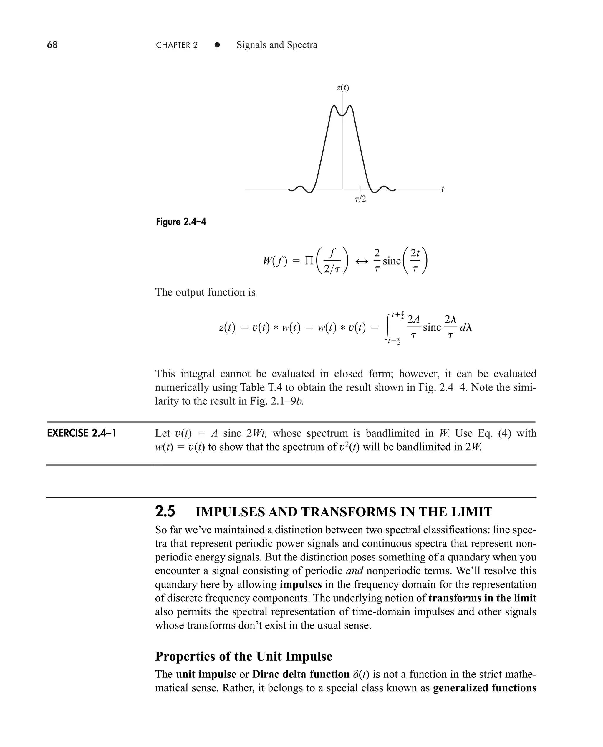
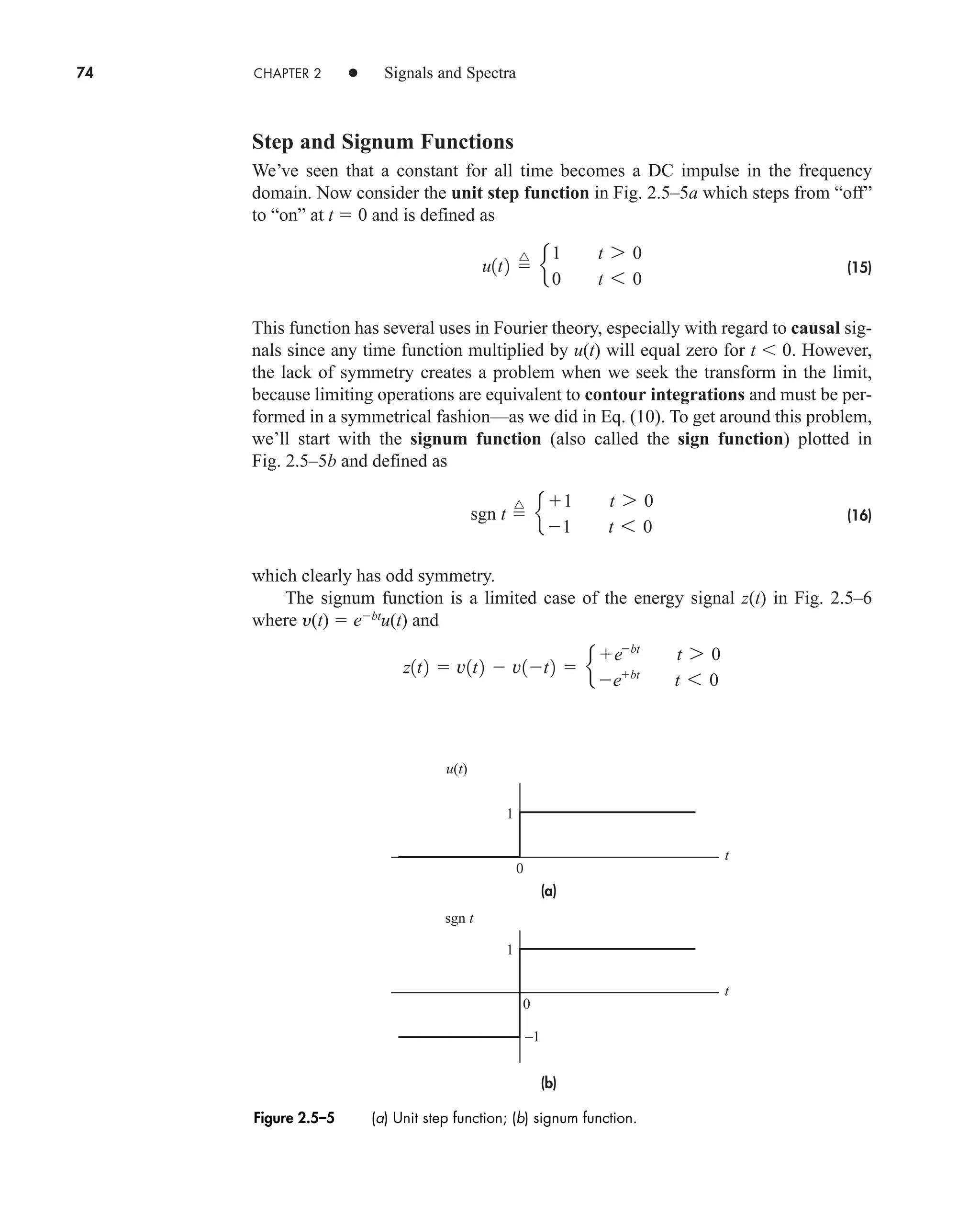
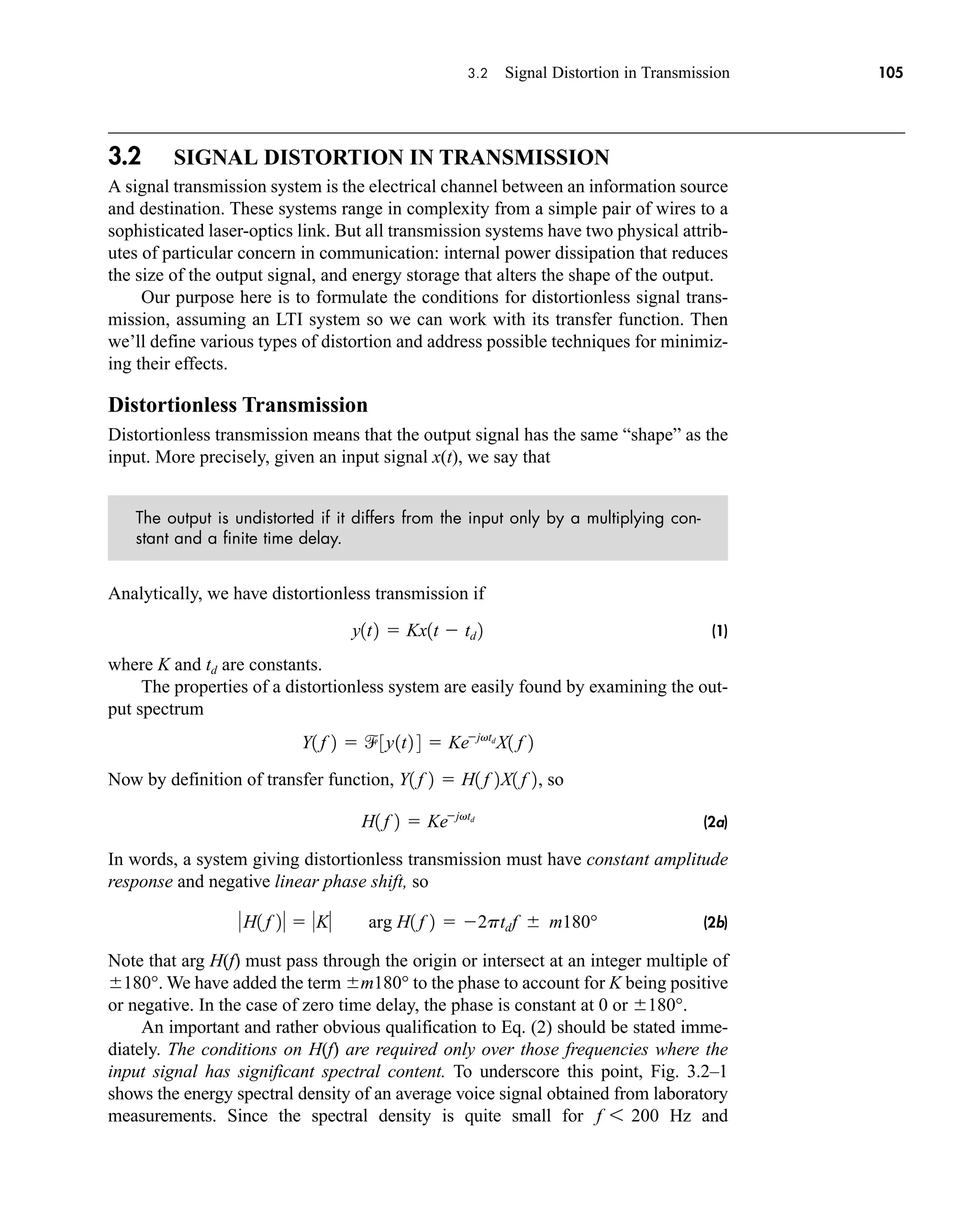
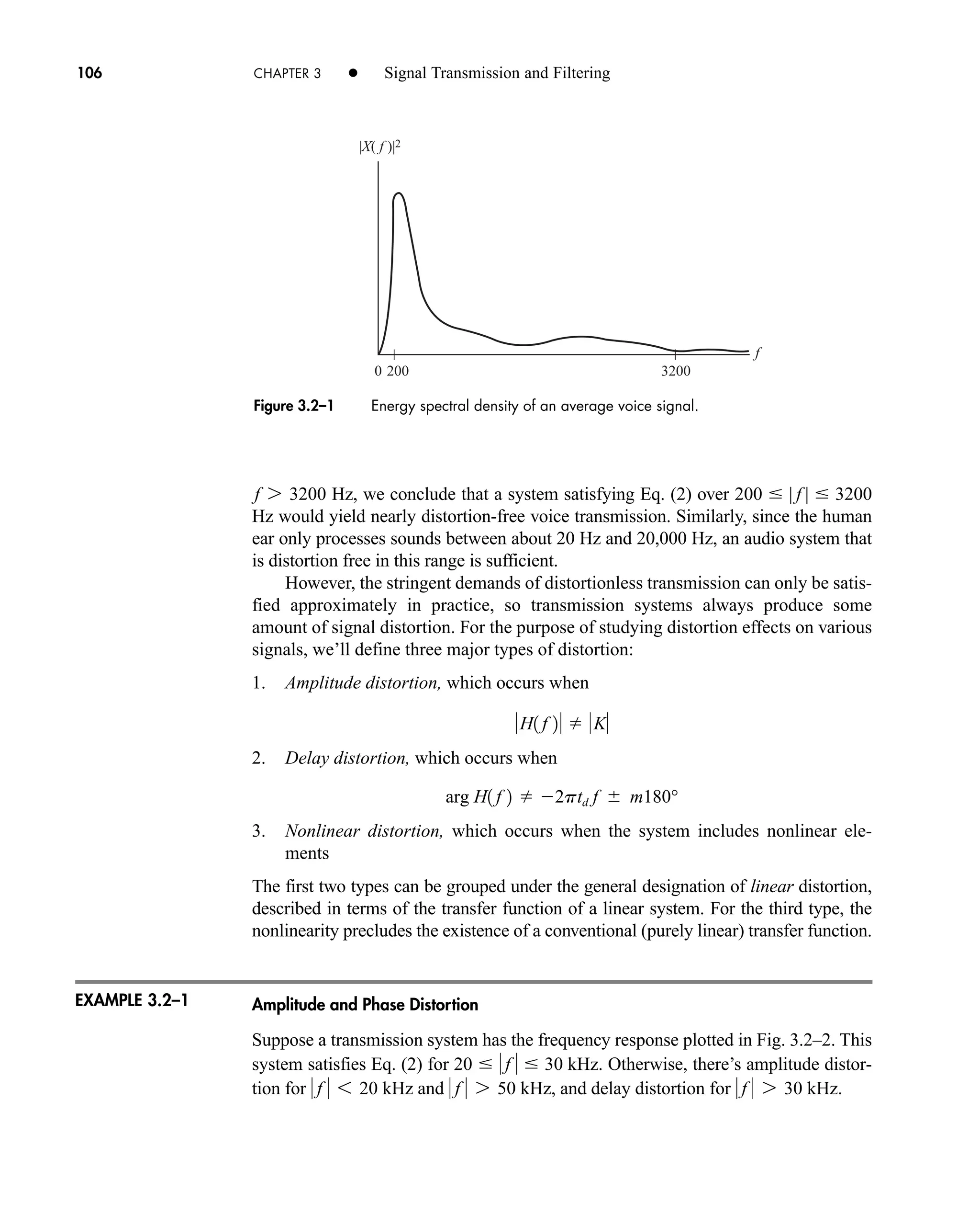
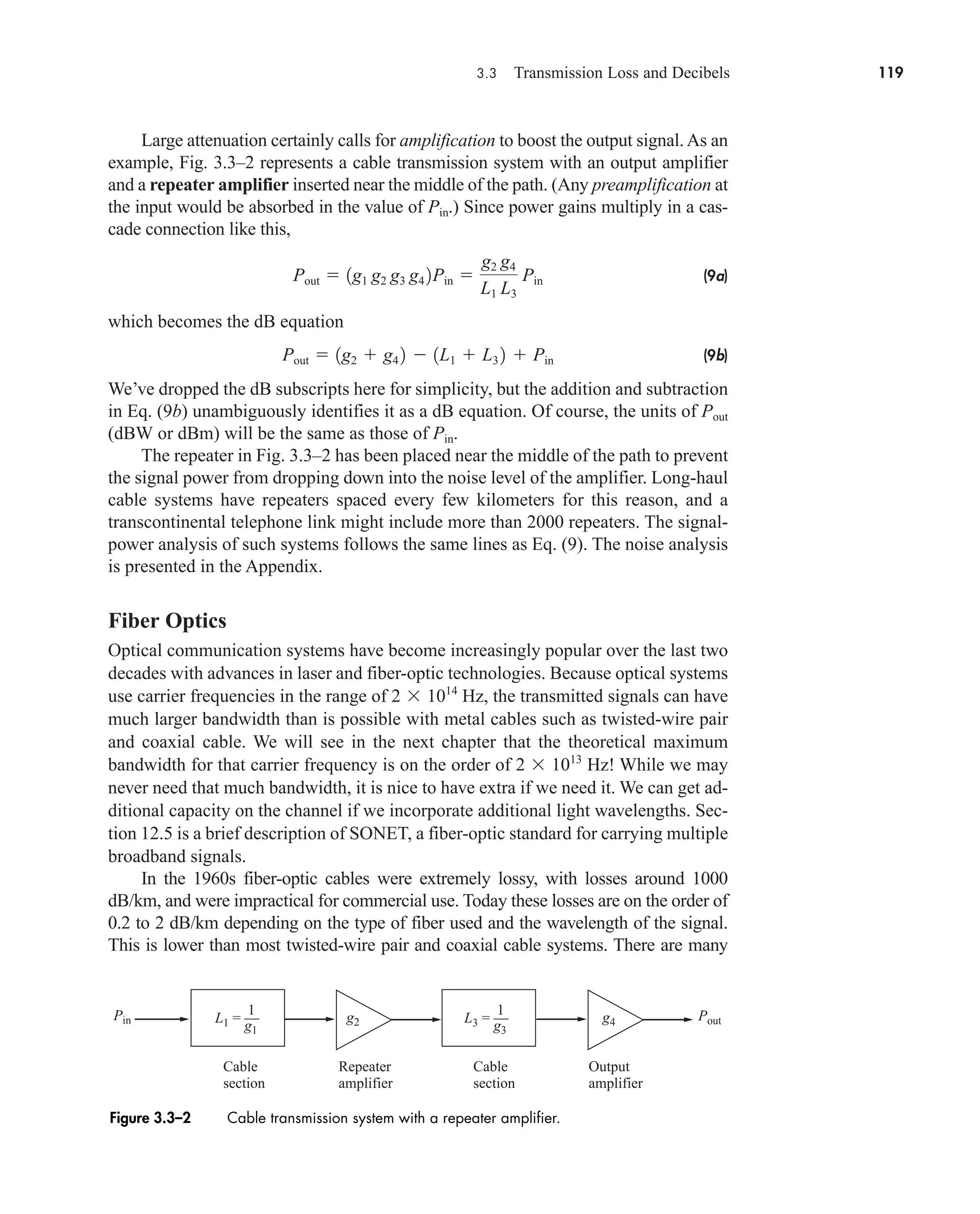
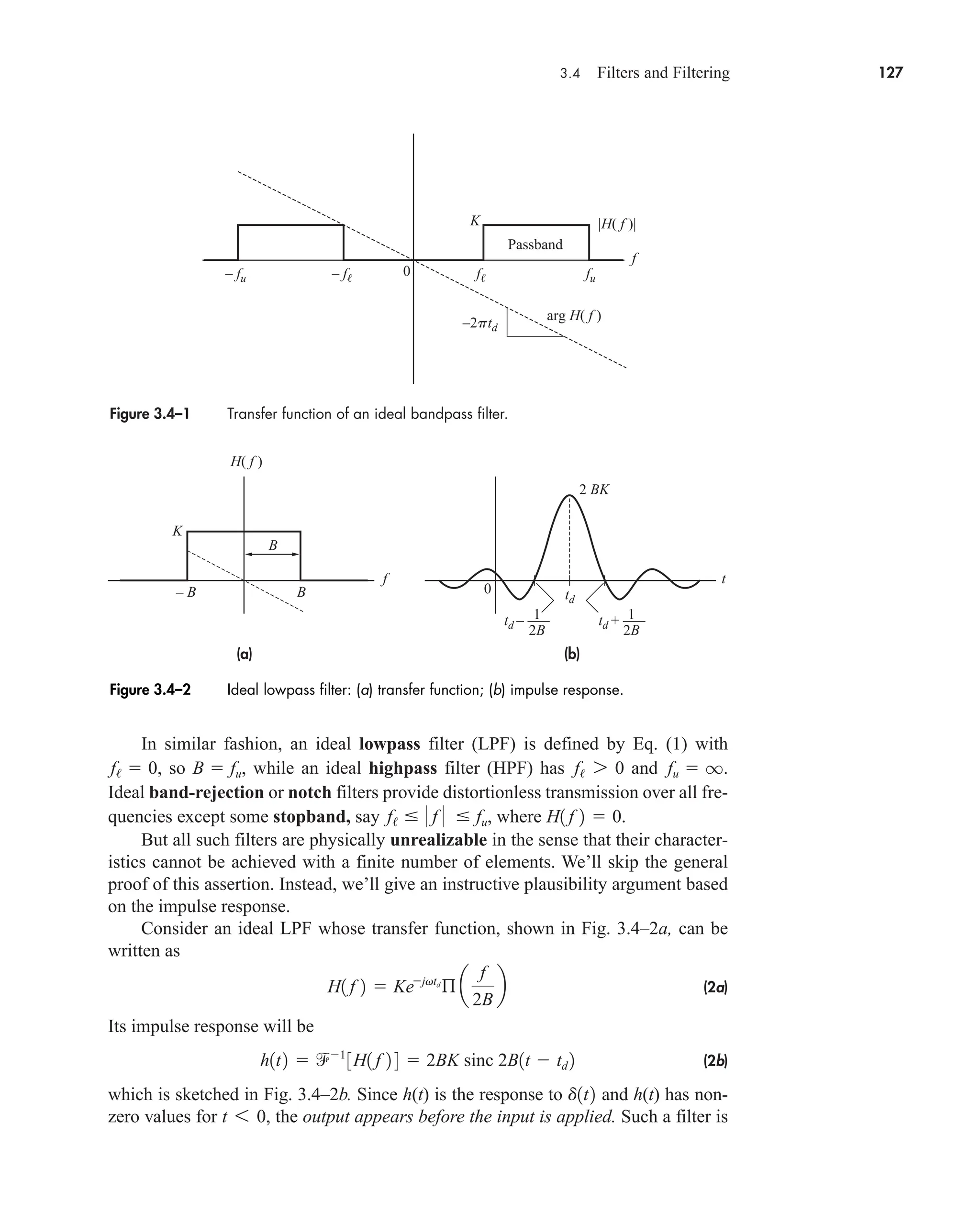
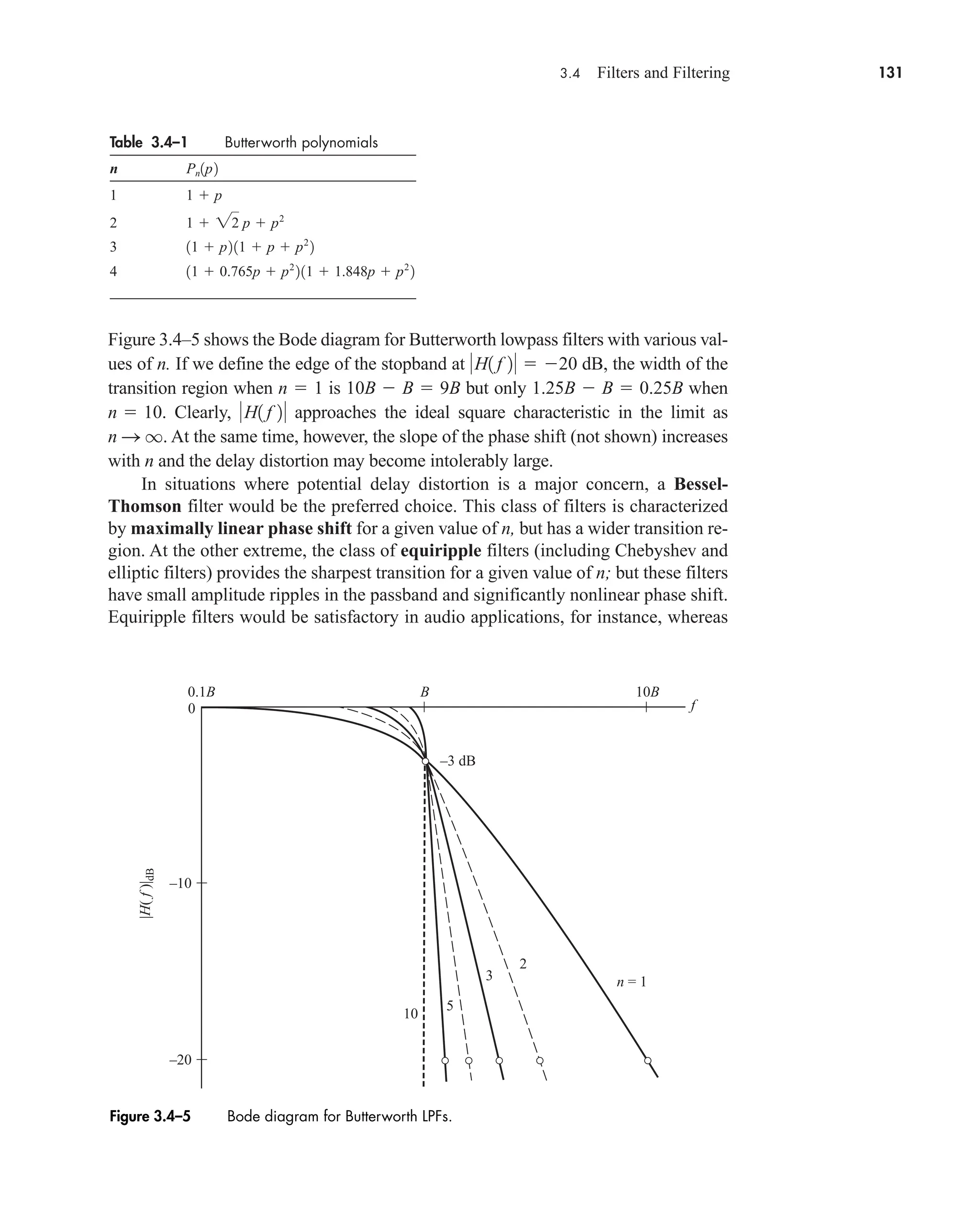
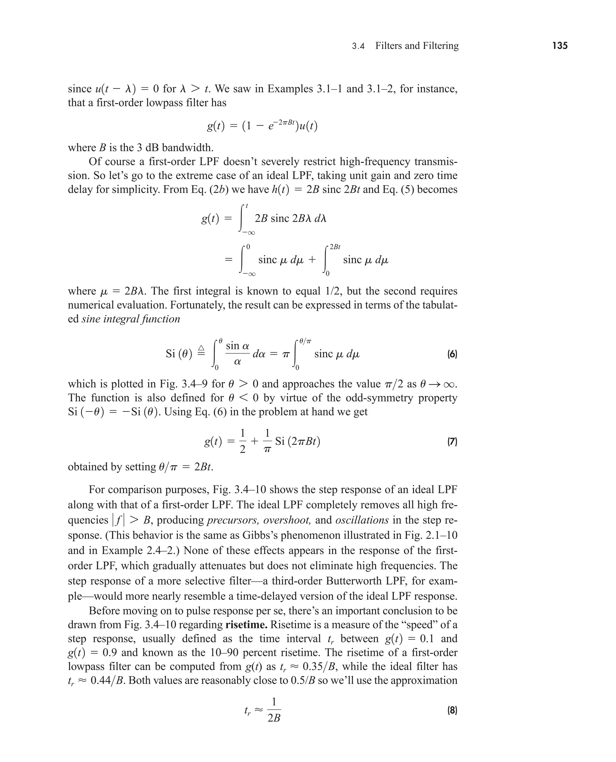
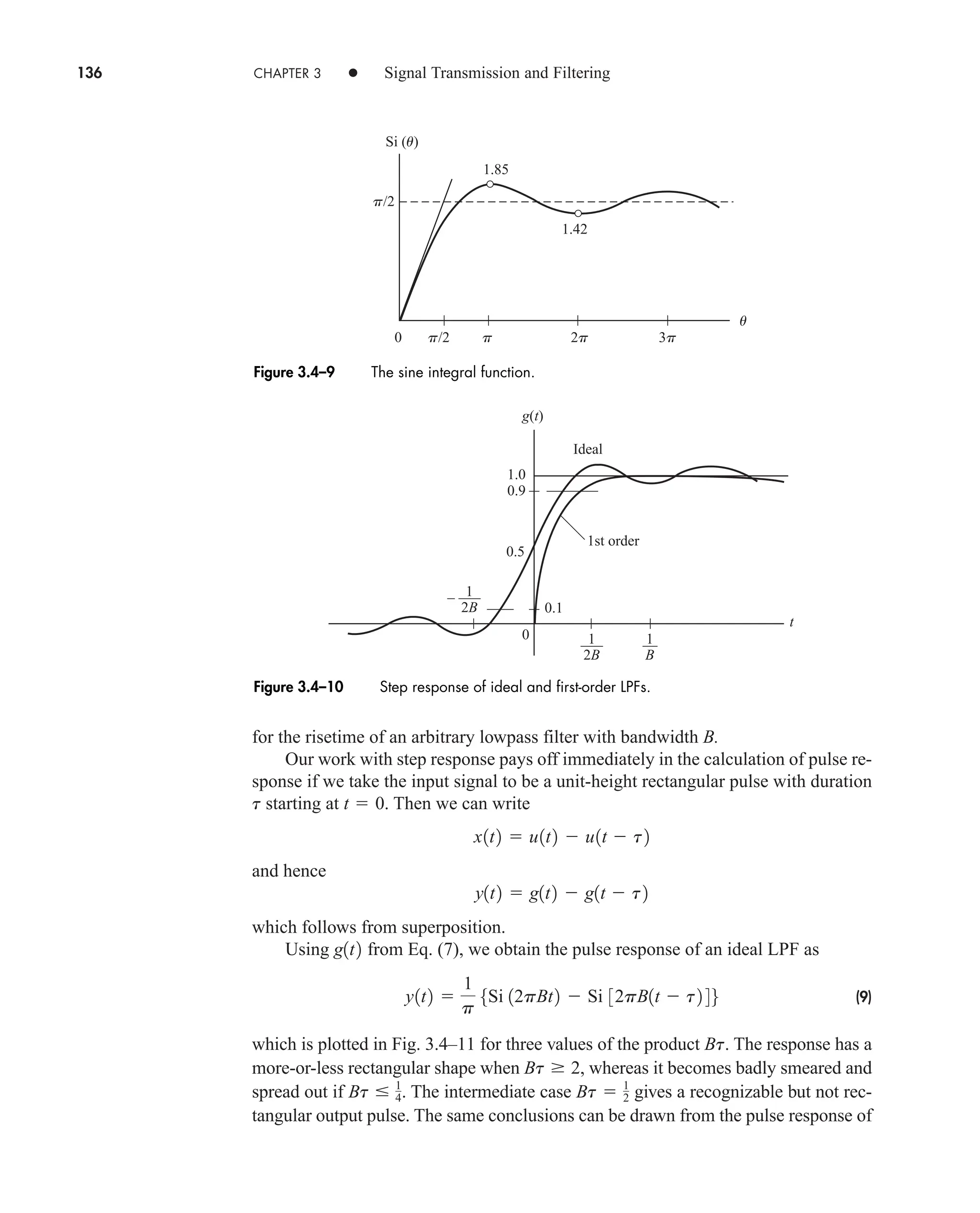
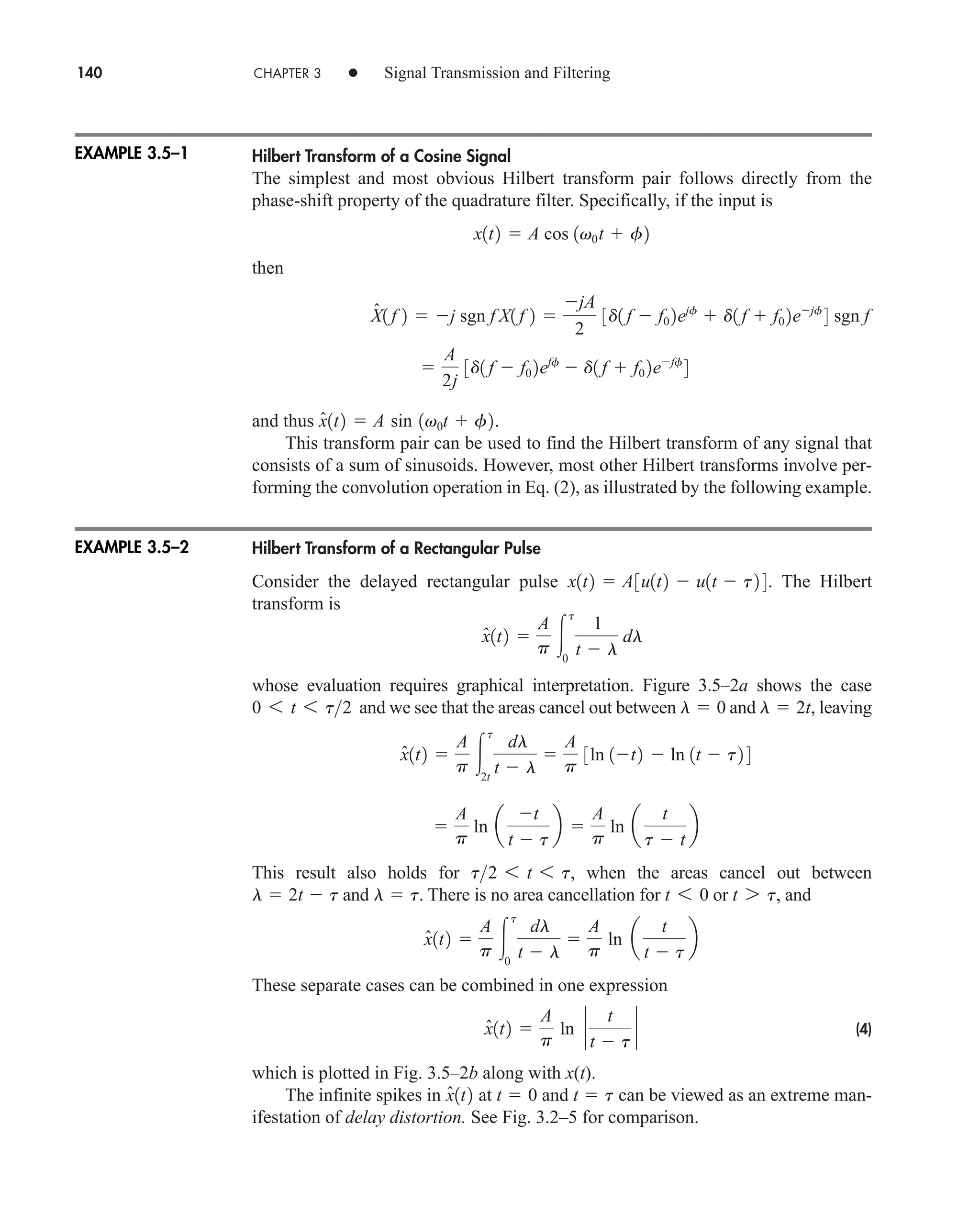
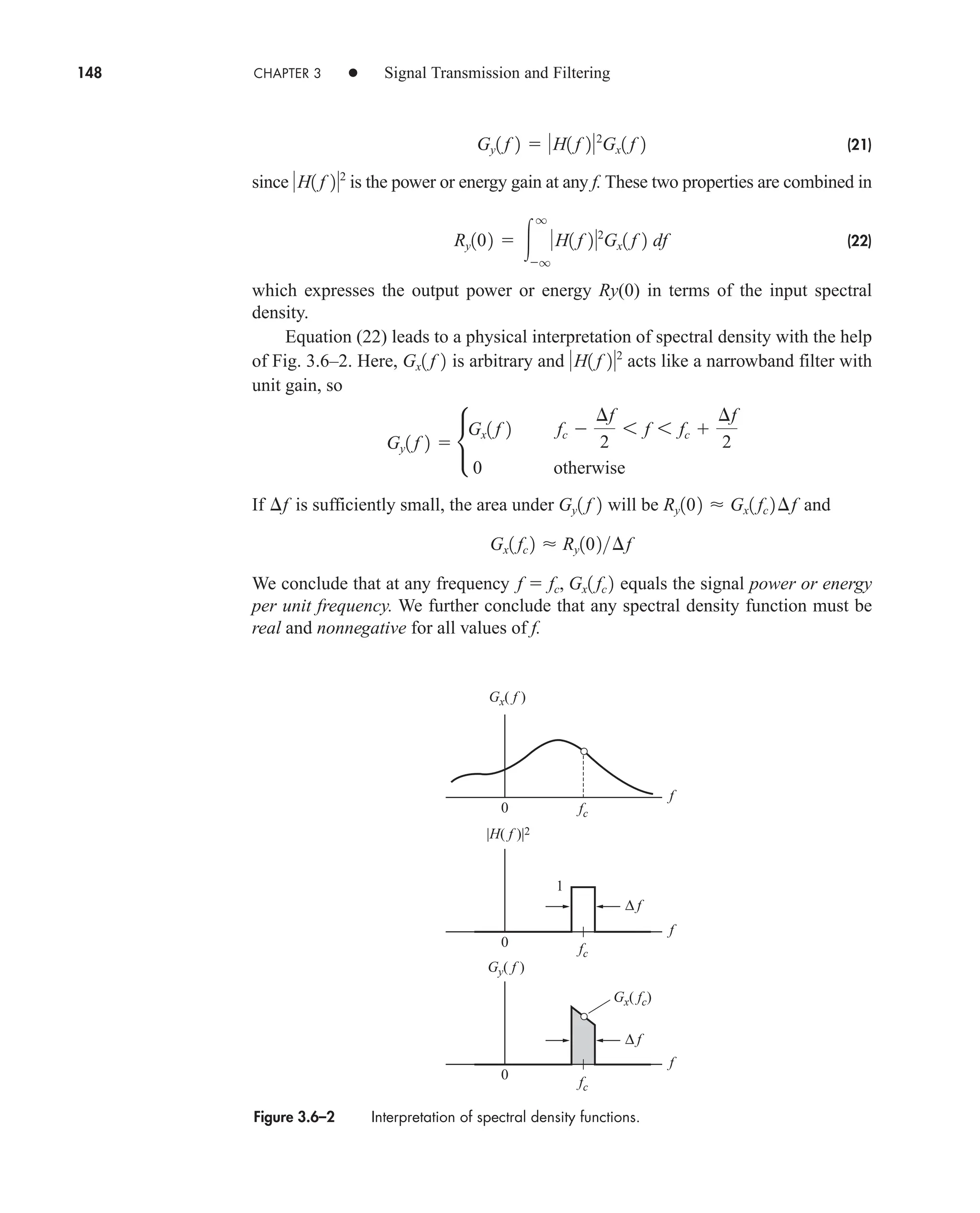
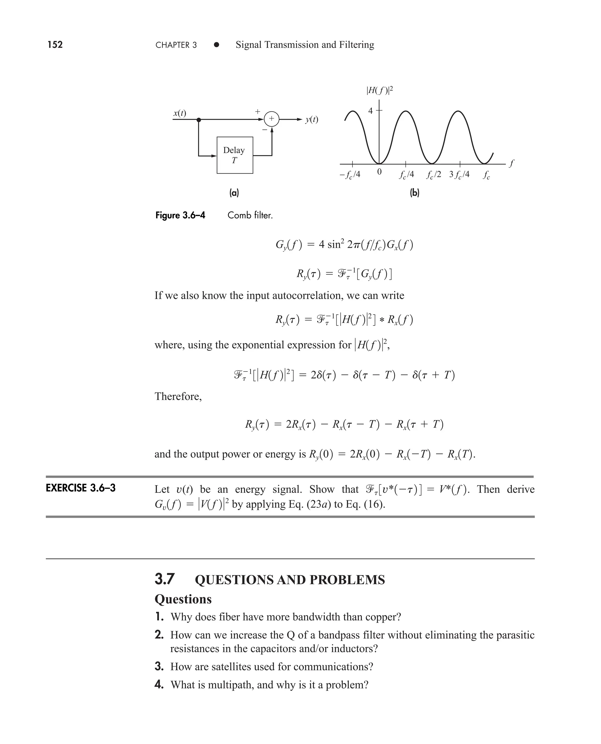
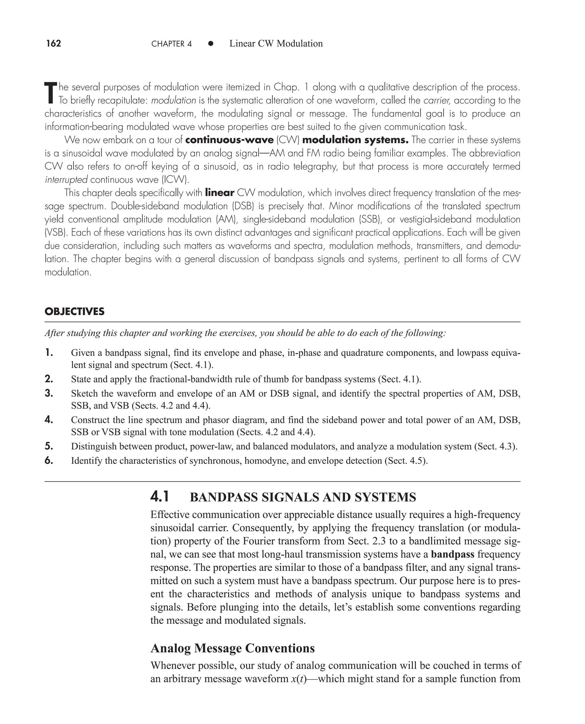
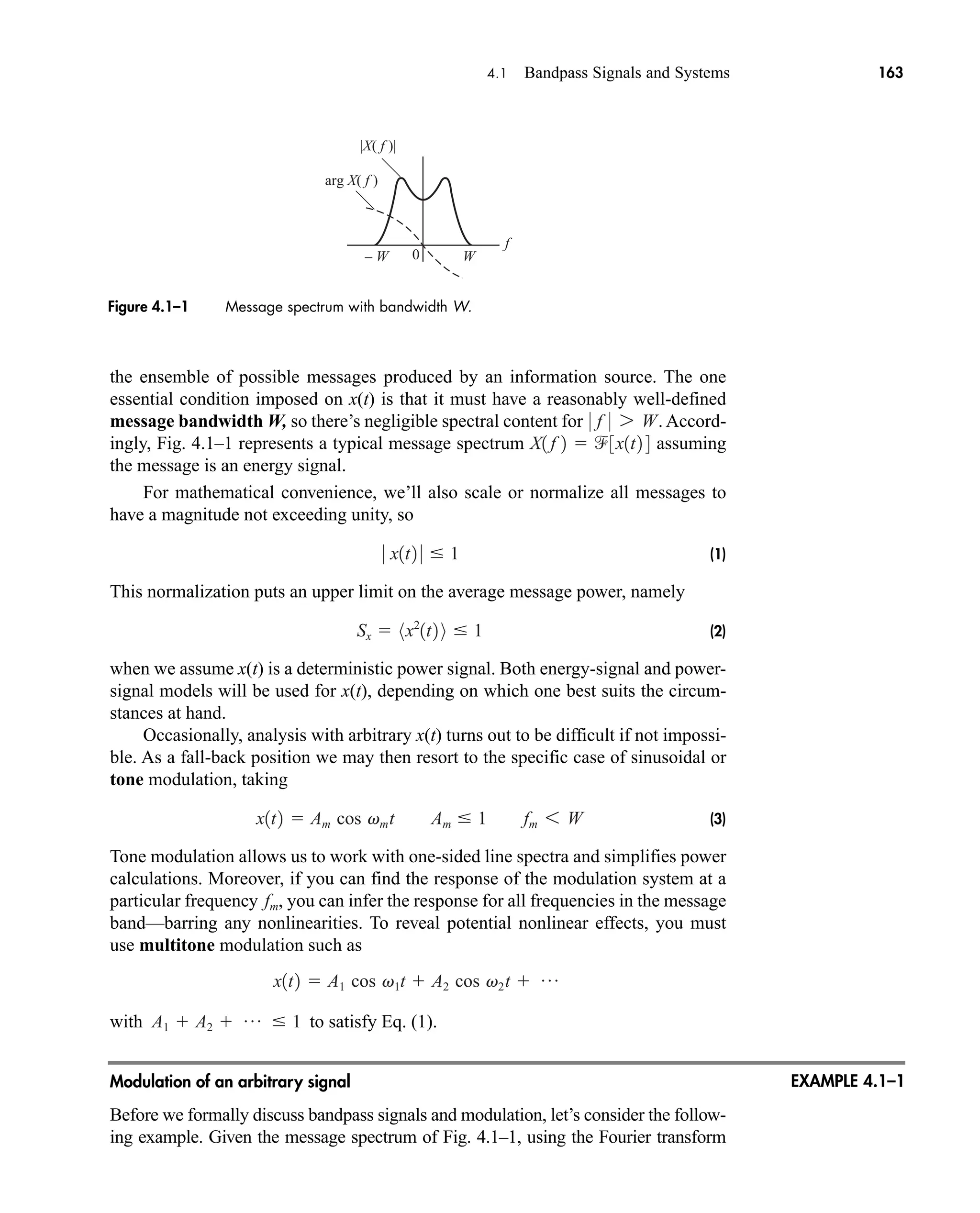
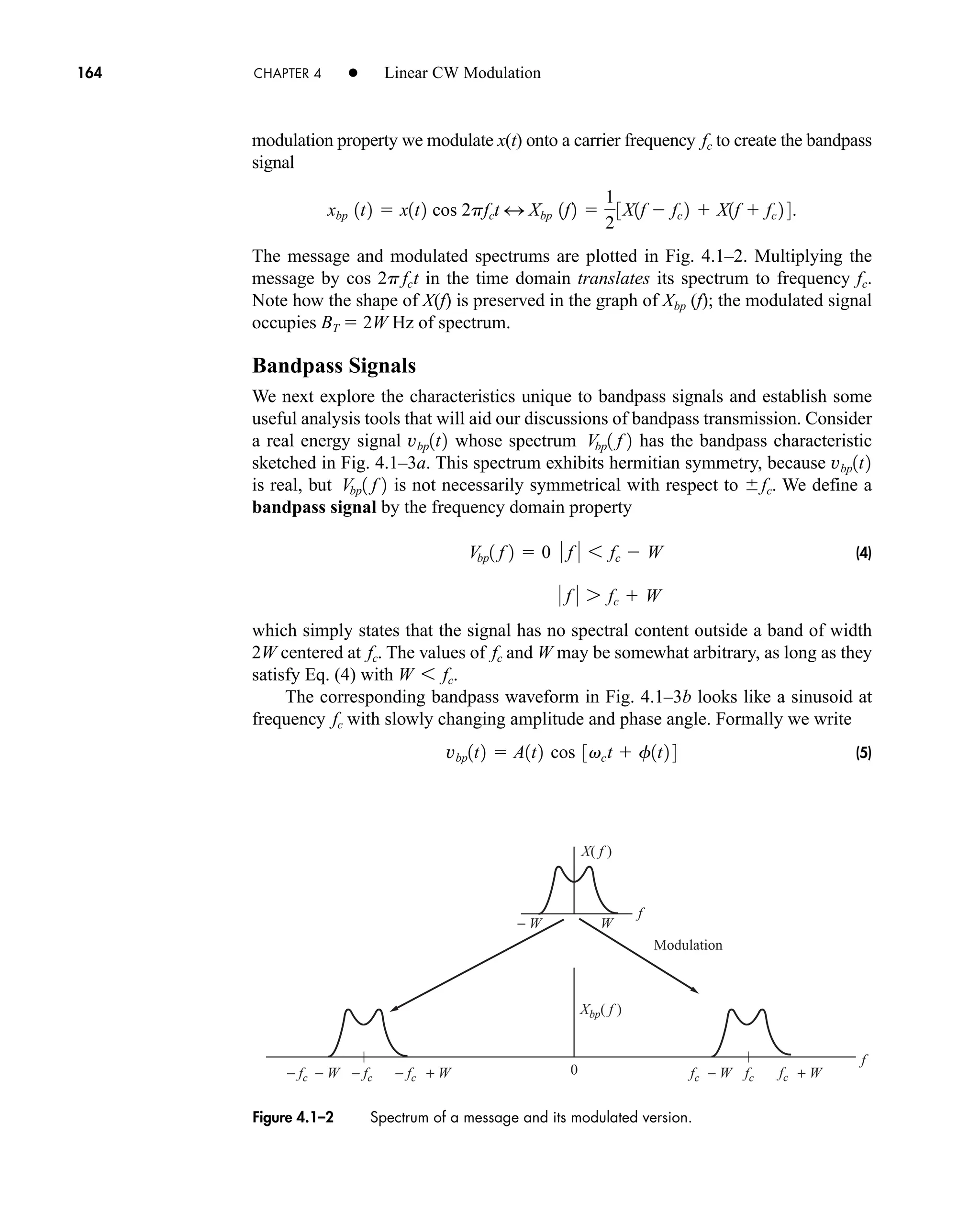
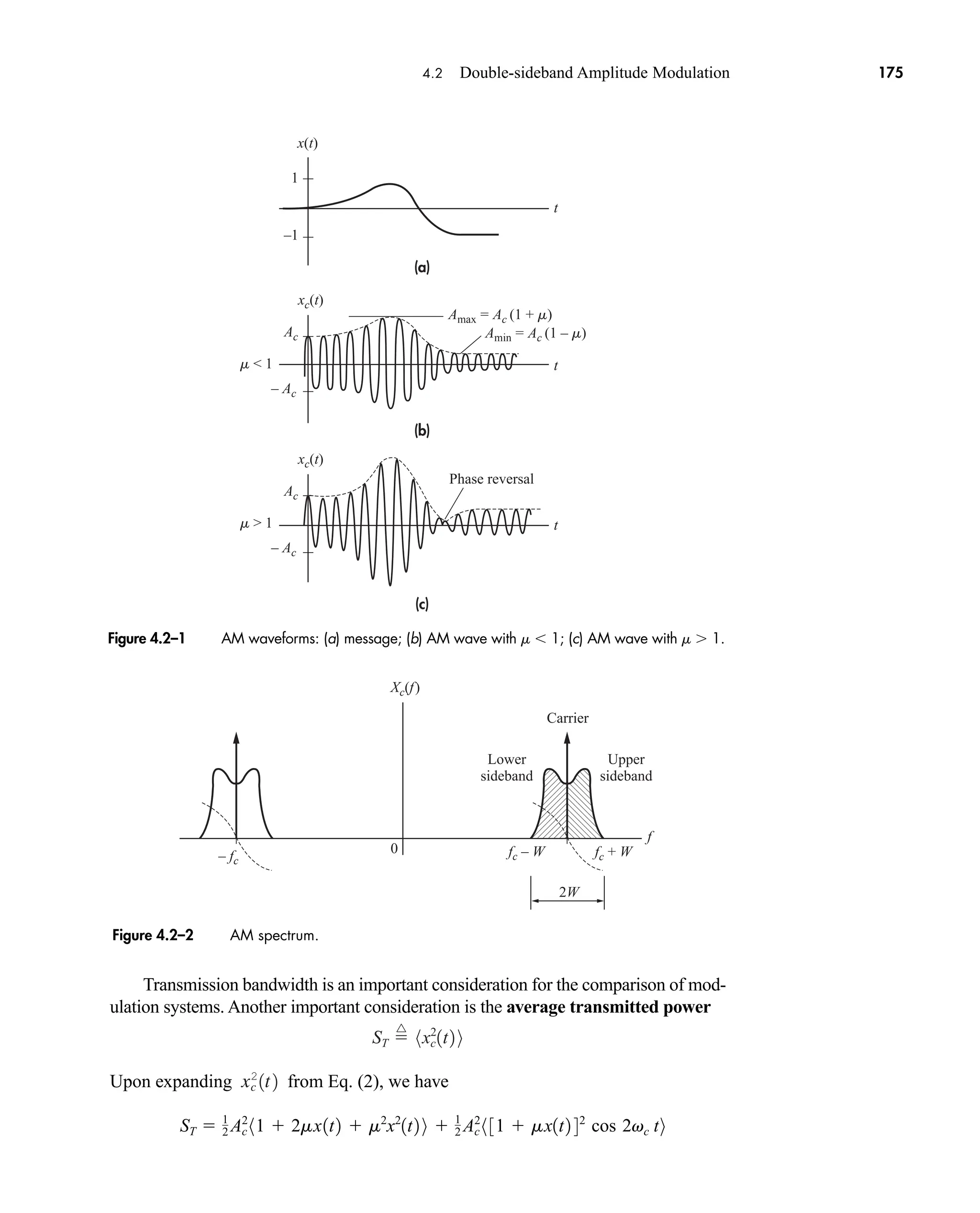
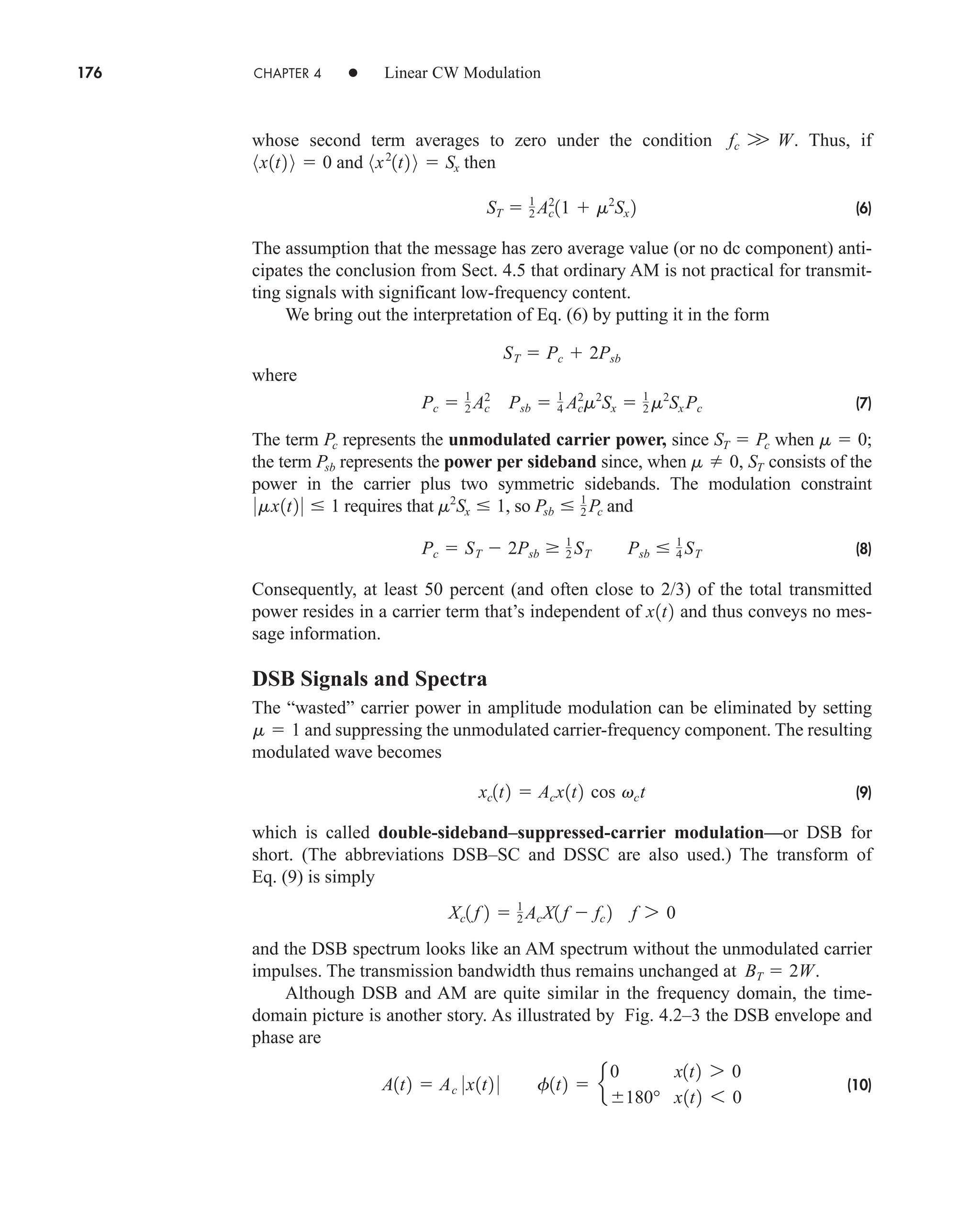
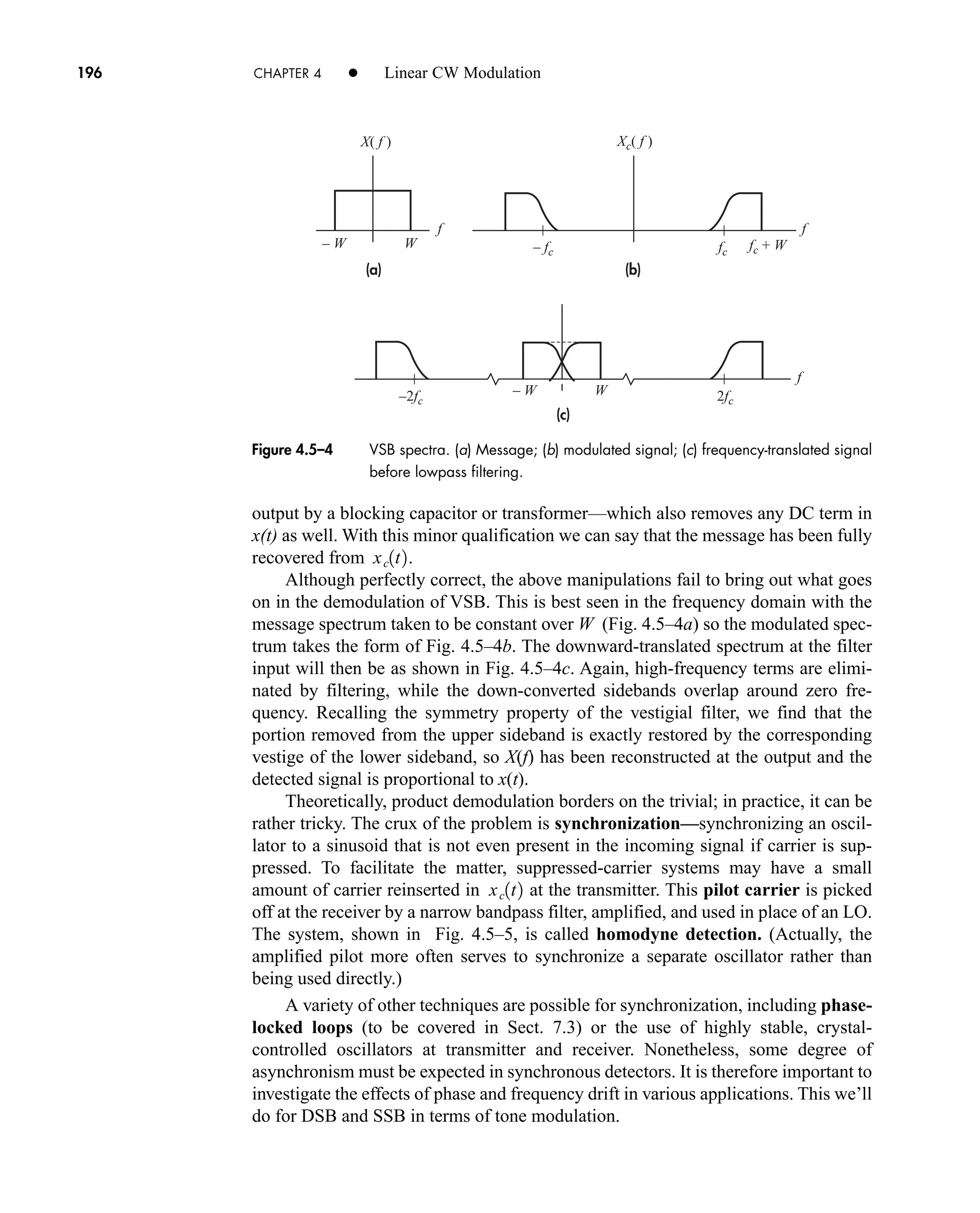
![36 CHAPTER 2 • Signals and Spectra
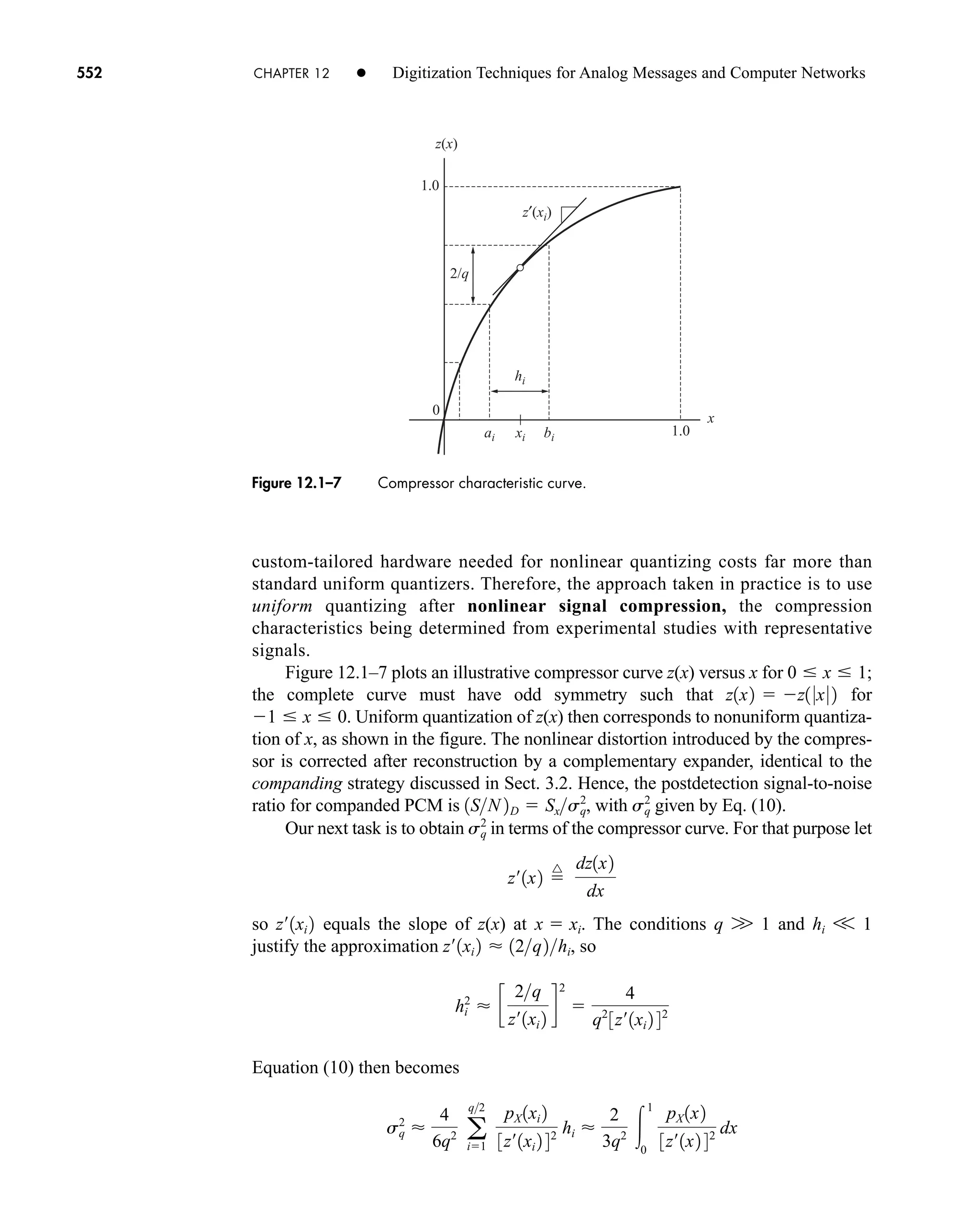
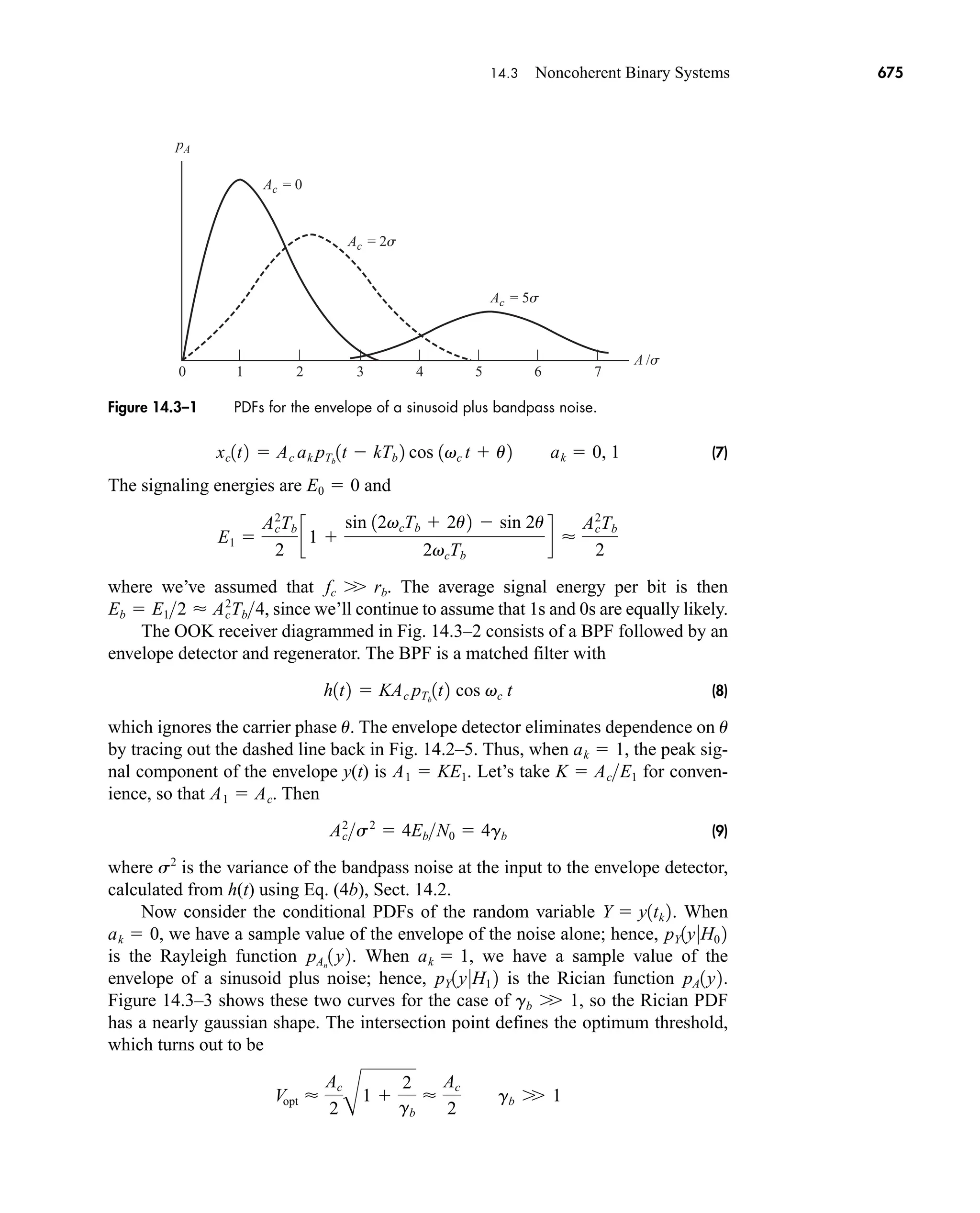
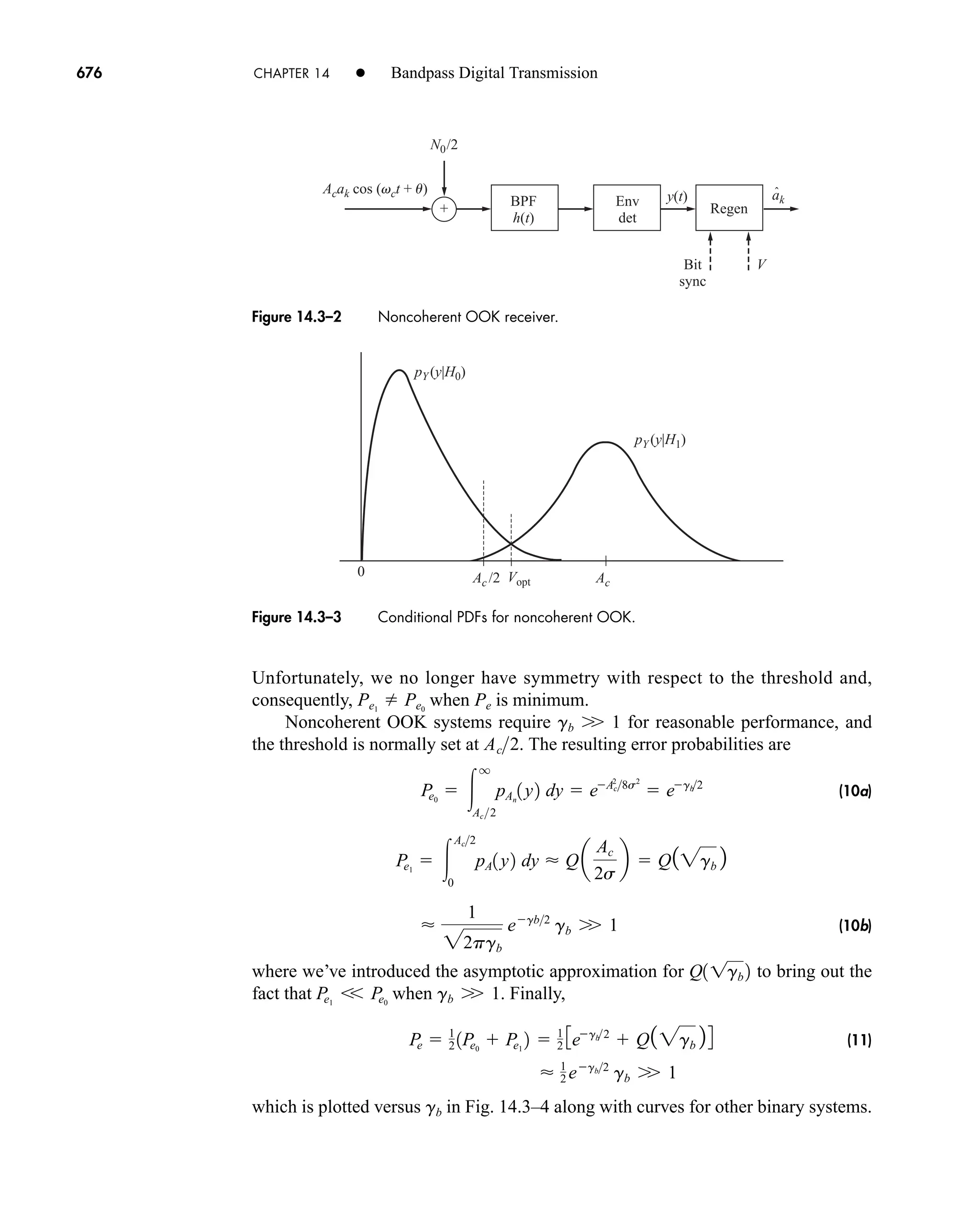
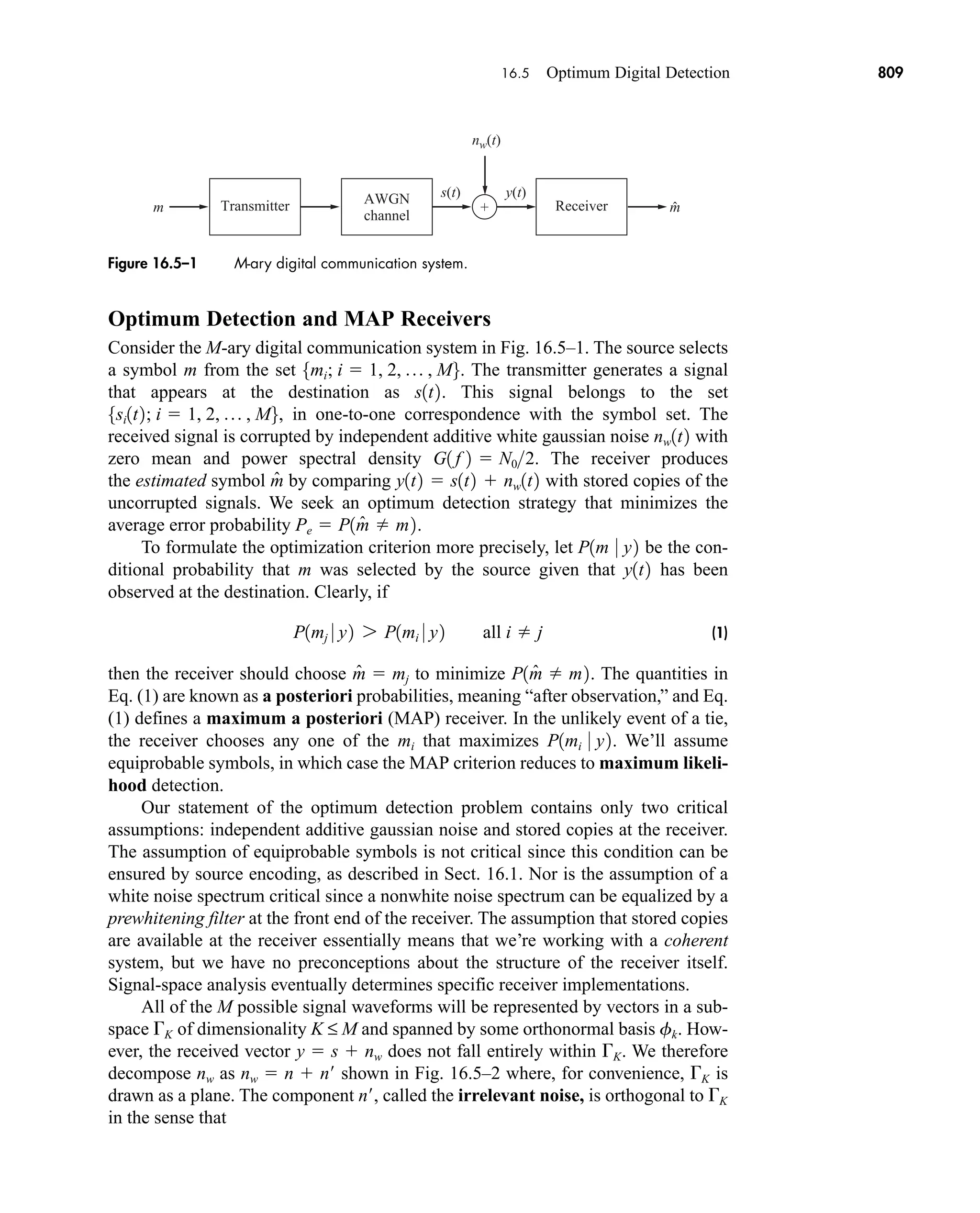
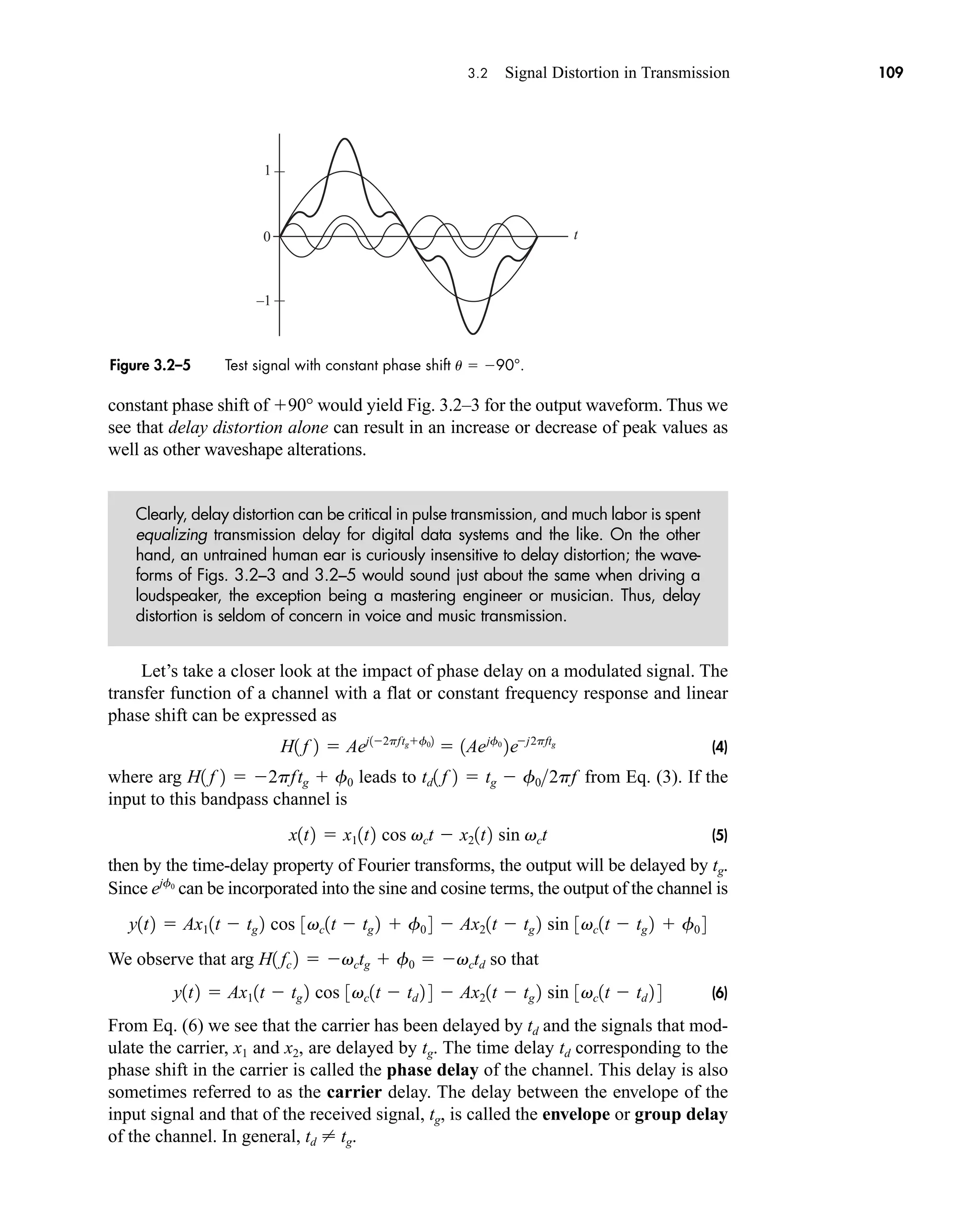
Calculated values of c(0) may be checked by inspecting v(t)—a wise practice
when the integration gives an ambiguous result.
3. If v(t) is a real (noncomplex) function of time, then
(16a)
which follows from Eq. (14) with n replaced by n. Hence
(16b)
which means that the amplitude spectrum has even symmetry and the phase
spectrum has odd symmetry.
When dealing with real signals, the property in Eq. (16) allows us to regroup the
exponential series into complex-conjugate pairs, except for c0. Equation (13) then
becomes
(17a)
or
(17b)
an Re[cn]
and bn Im[cn]. Re[ ] and Im[ ] being the real and imaginary operators respectively.
Equation 17a is the trigonometric Fourier Series and suggests a one-sided
spectrum. Most of the time, however, we’ll use the exponential series and two-sided
spectra.
The sinusoidal terms in Eq. (17) represent a set of orthogonal basis functions.
Functions vn(t) and vm(t) are orthogonal over an interval from t1 to t2 if
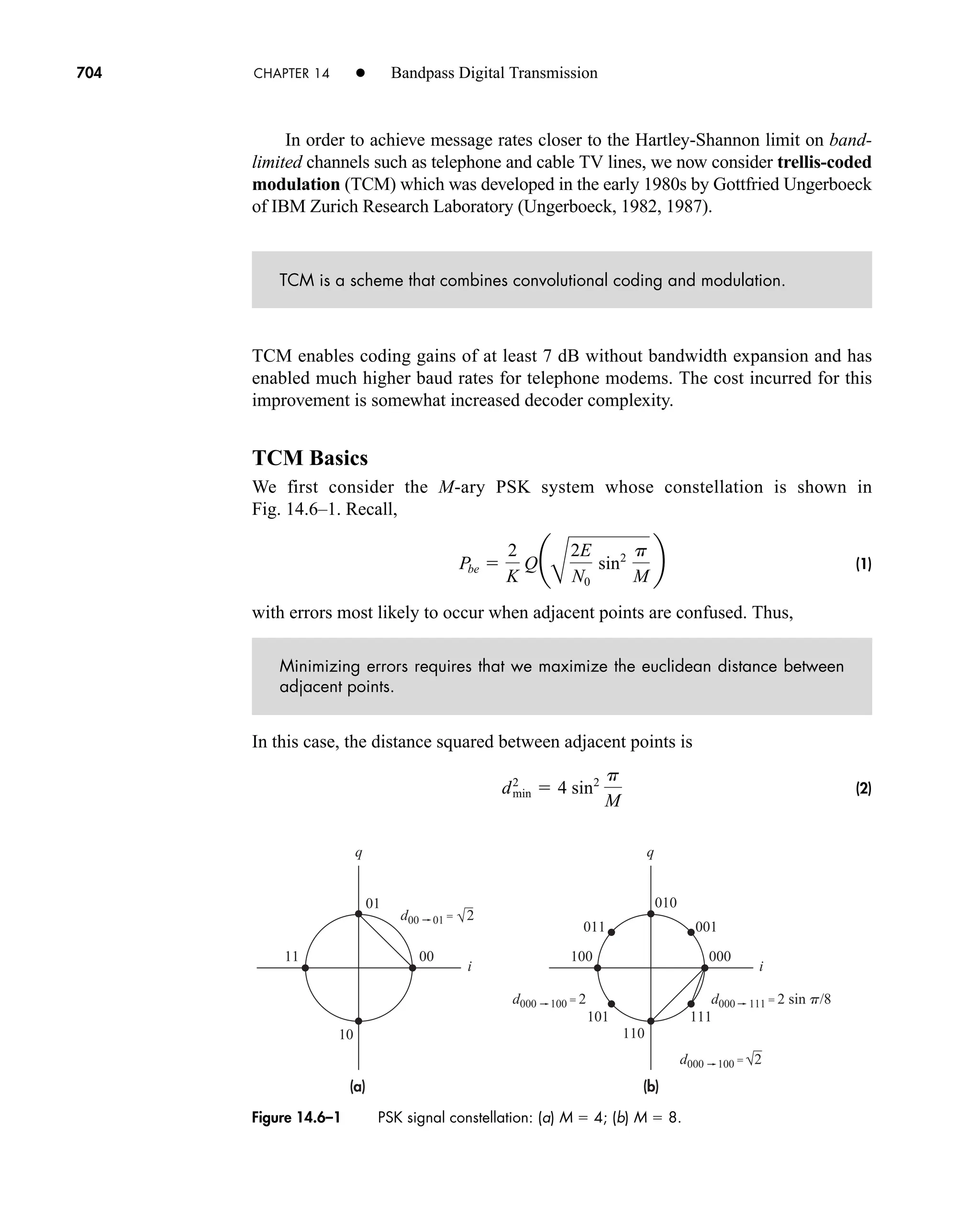
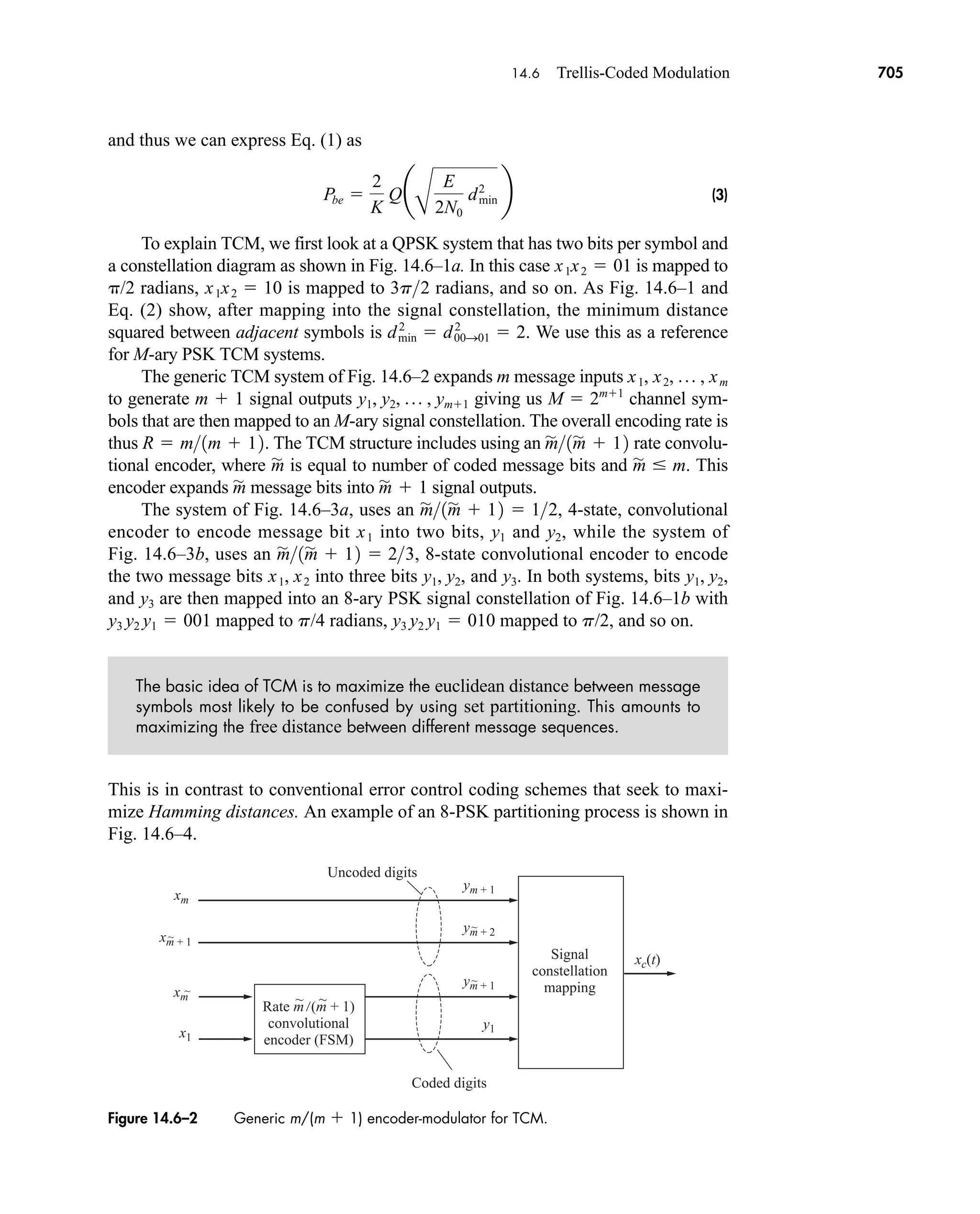
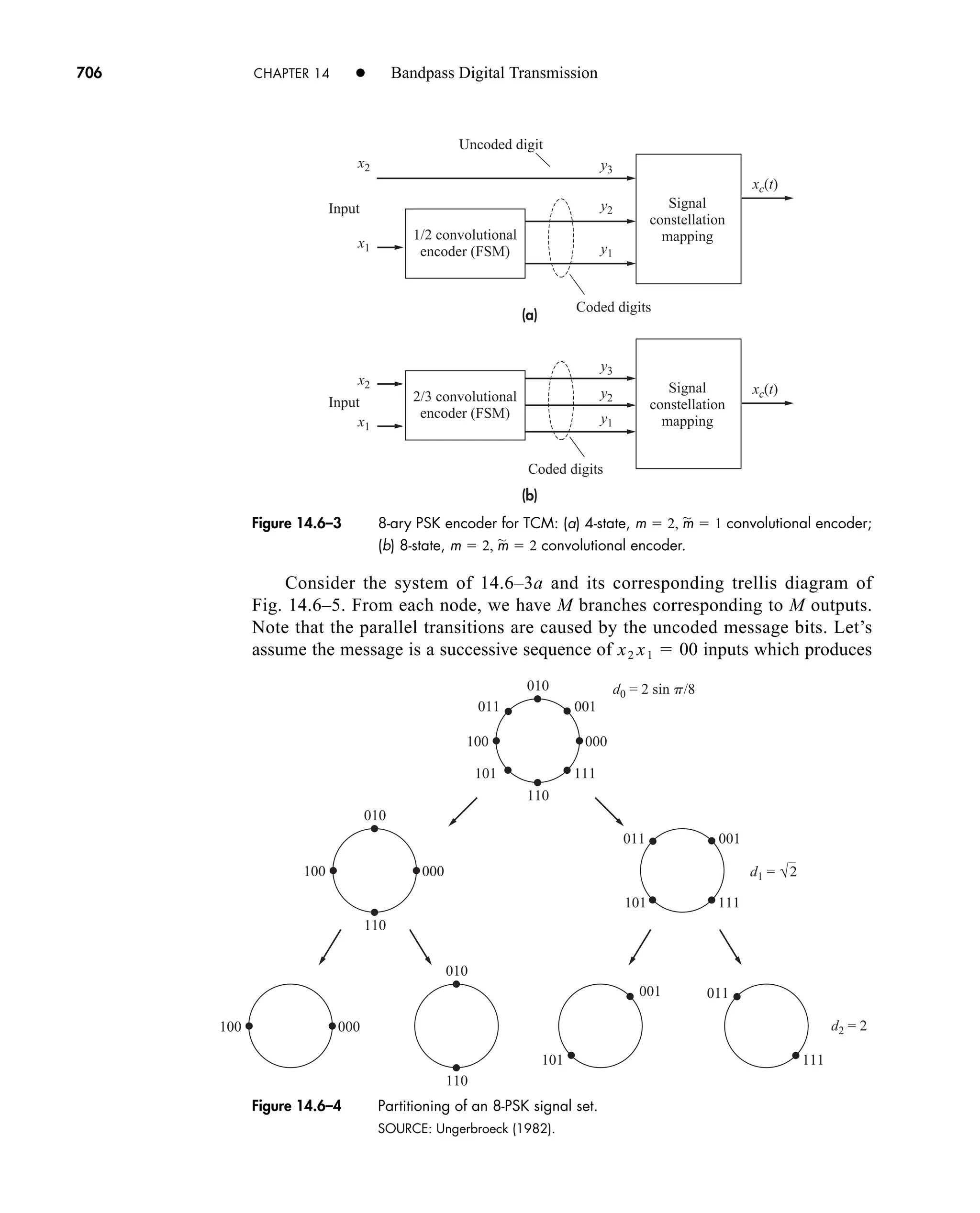
Later we will see in Sect. 7.2 (QAM) and 14.5 that a set of users can share a
channel without interfering with each other by using orthogonal carrier signals.
One final comment should be made before taking up an example. The integra-
tion for cn often involves a phasor average in the form
(18)
Since this expression occurs time and again in spectral analysis, we’ll now introduce
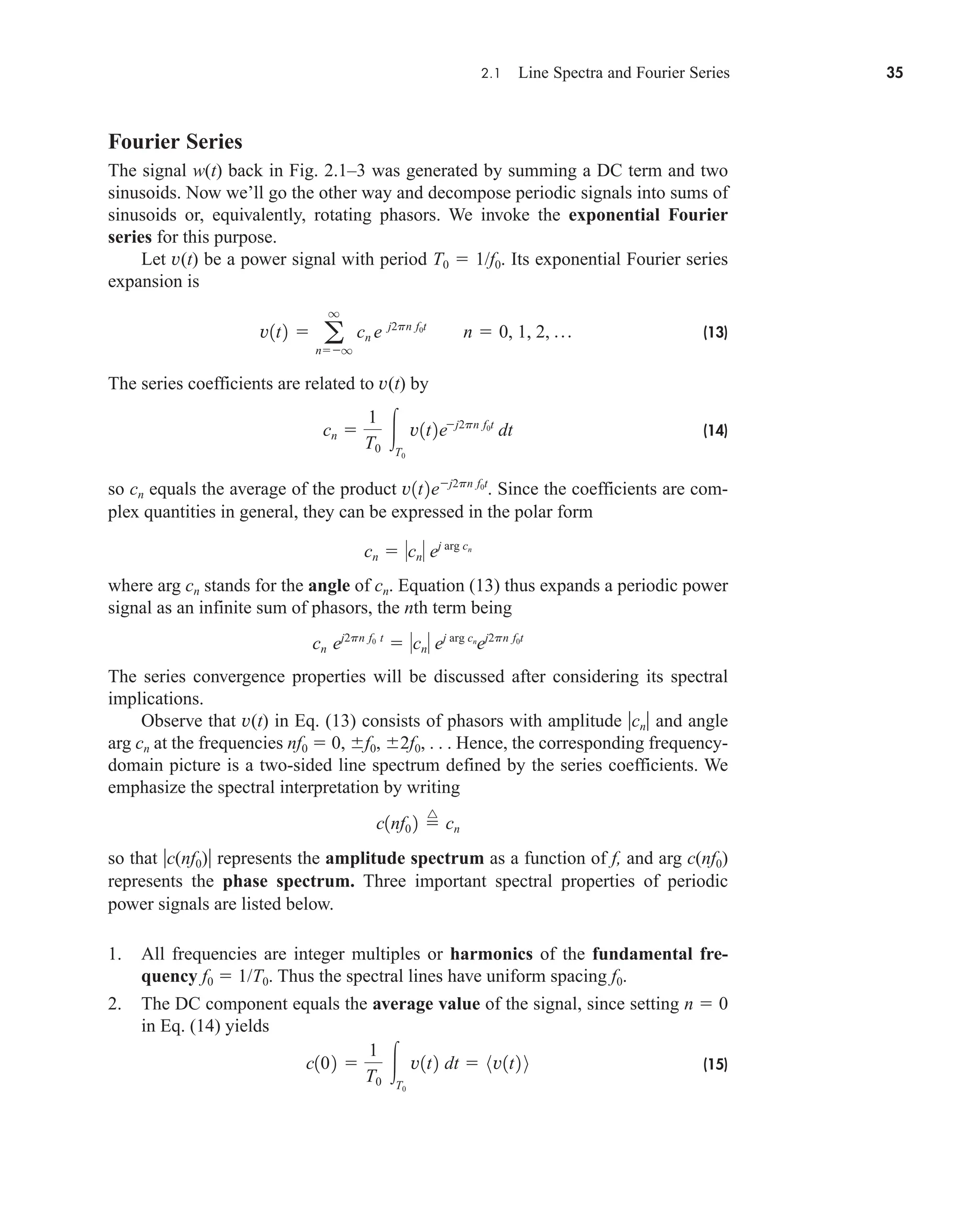
the sinc function defined by
1
pf T
sin pf T
1
T
T2
T2
ej2pft
dt
1
j2pf T
1ejpf T
ejpf T
2
t2
t1
vn1t2vm1t2dt e
0 n m
K n m
with K a constant.
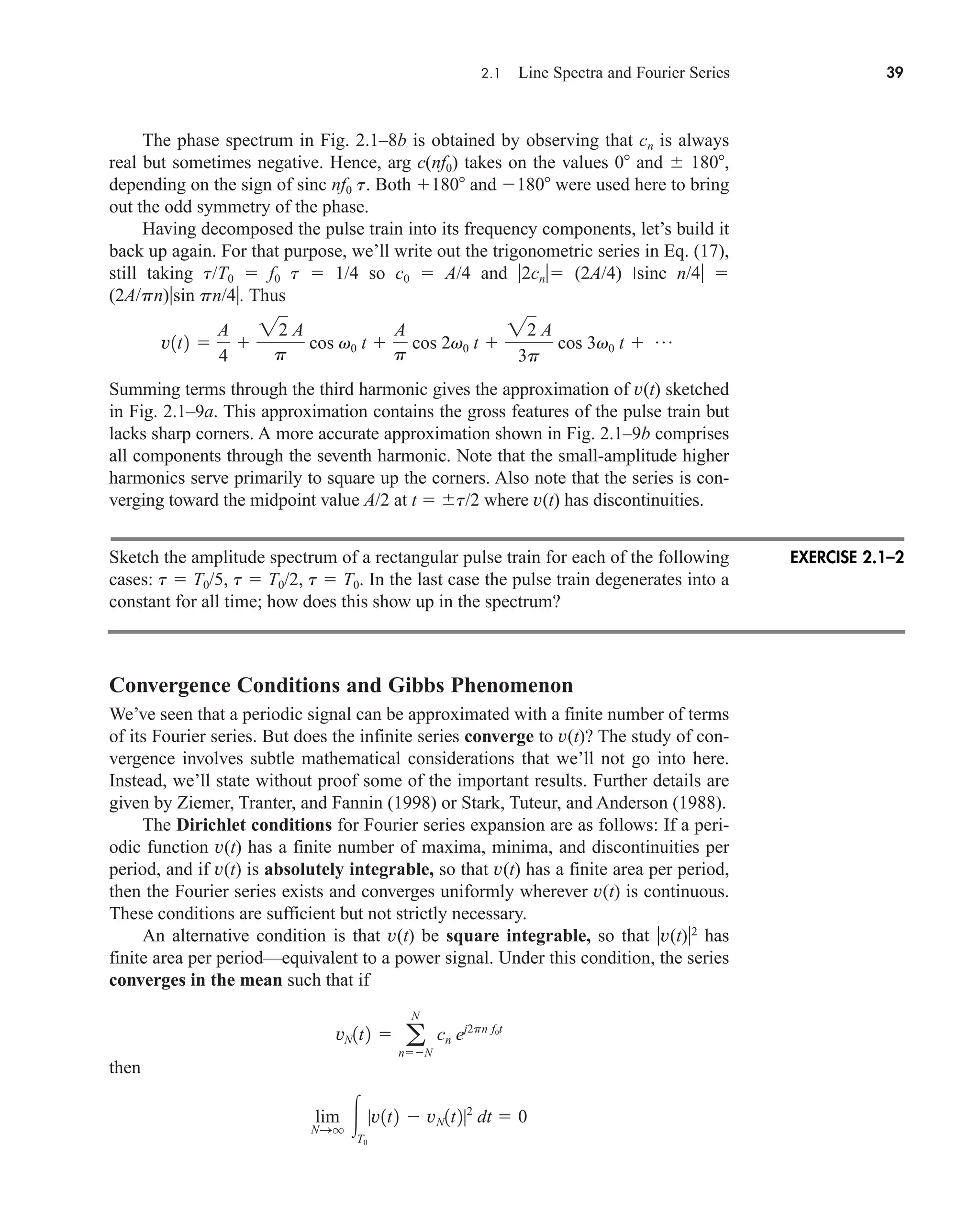
v1t2 c0 a
q
n1
3an cos 2pnf0t bn sin 2pf0t4
v1t2 c0 a
q
n1
2cn cos12pnf0t arg cn 2
c1nf0 2 c1nf0 2 arg c1nf0 2 arg c1nf0 2
cn c*
n cn ej arg cn
car80407_ch02_027-090.qxd 12/8/08 11:03 PM Page 36](https://image.slidesharecdn.com/communicationsystemsanintro-a-241115060943-61721fa8/75/Communication_Systems__An_Intro_-_A-_Bruce_Carlson_-pdf-58-2048.jpg)
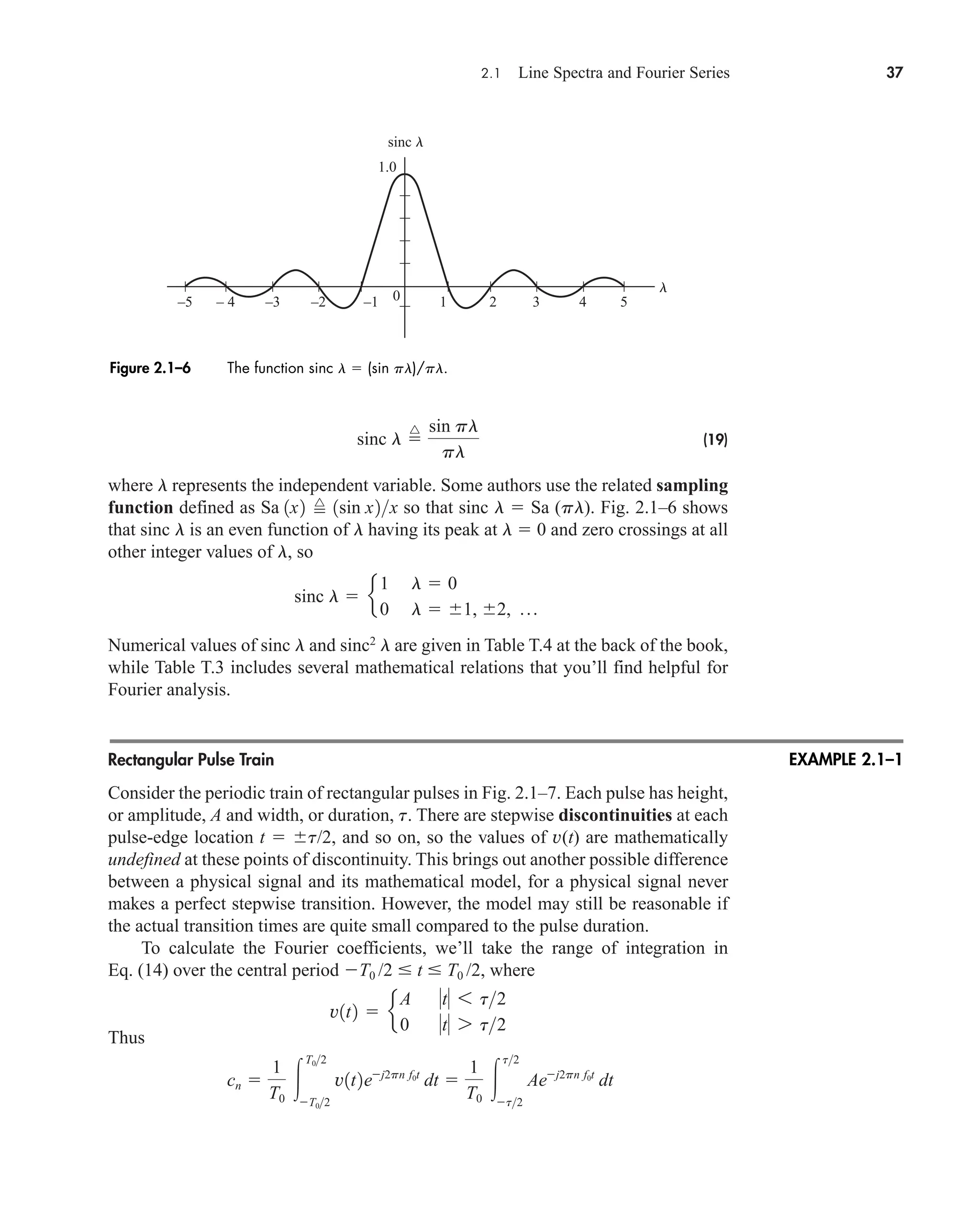
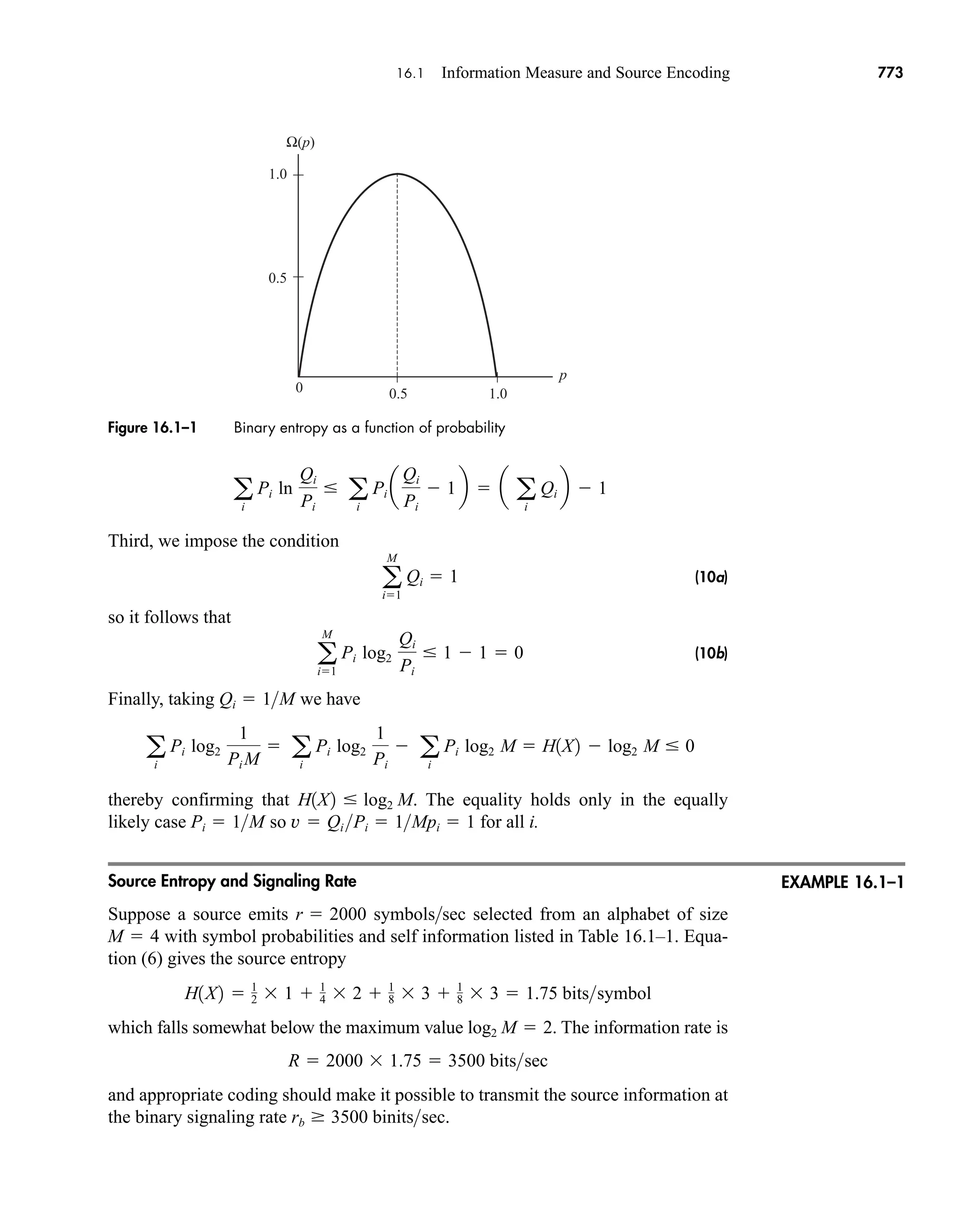
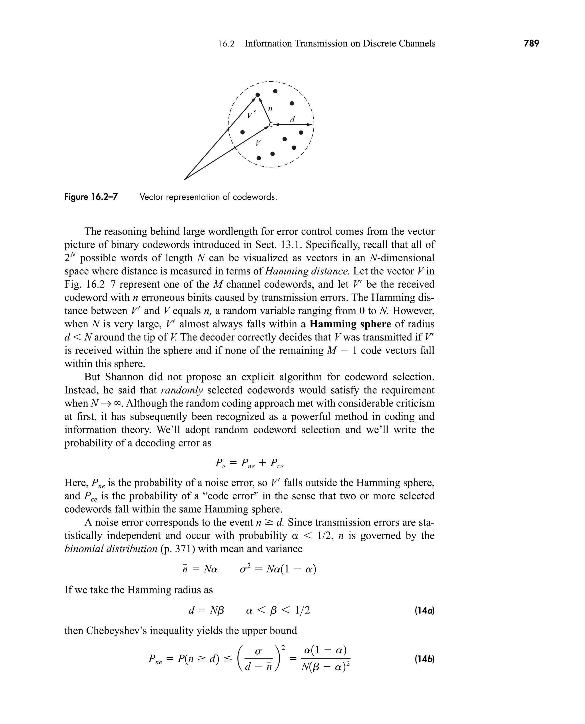
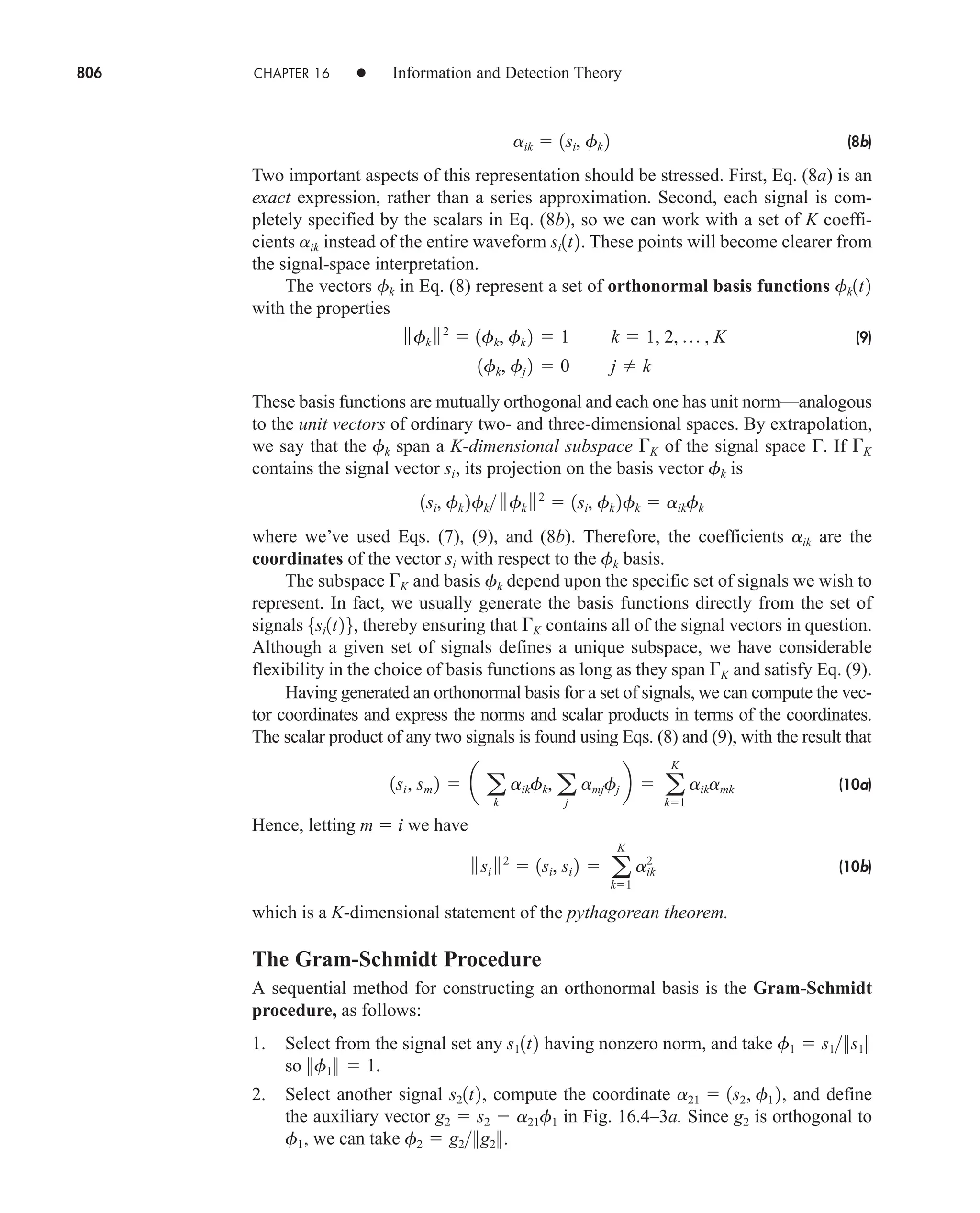
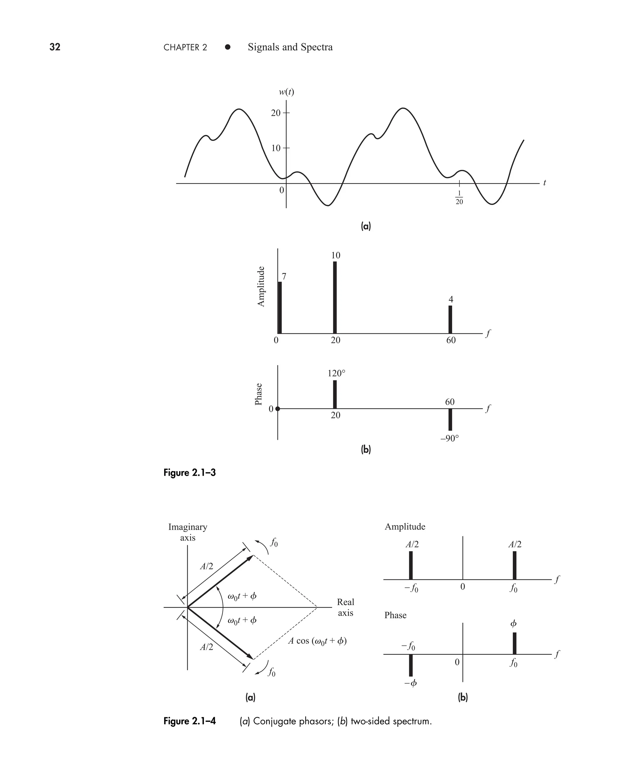
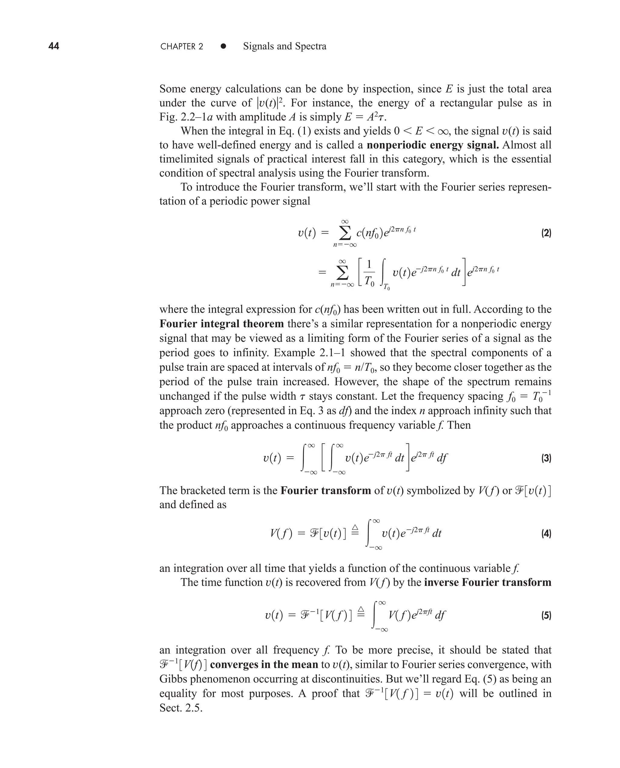
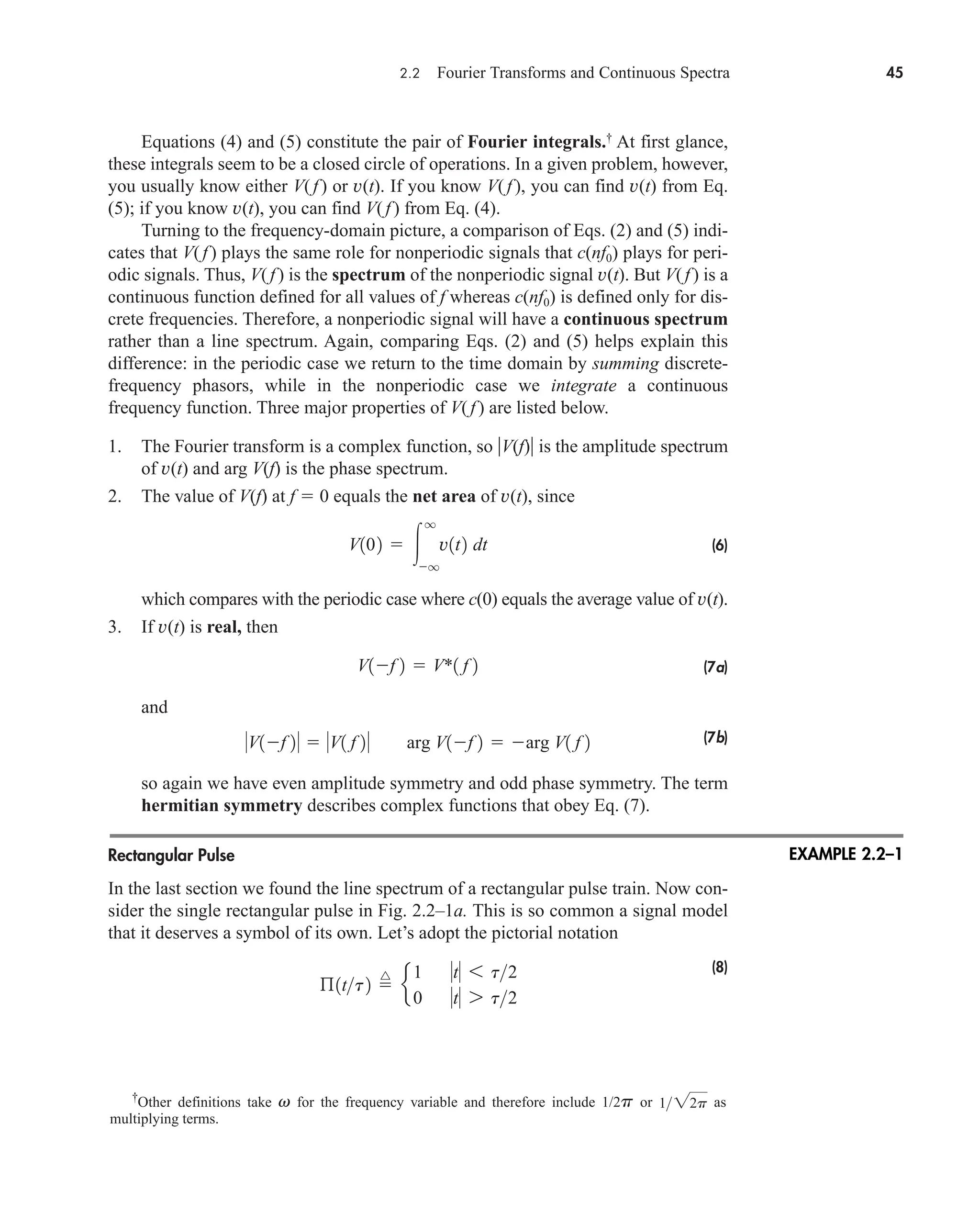
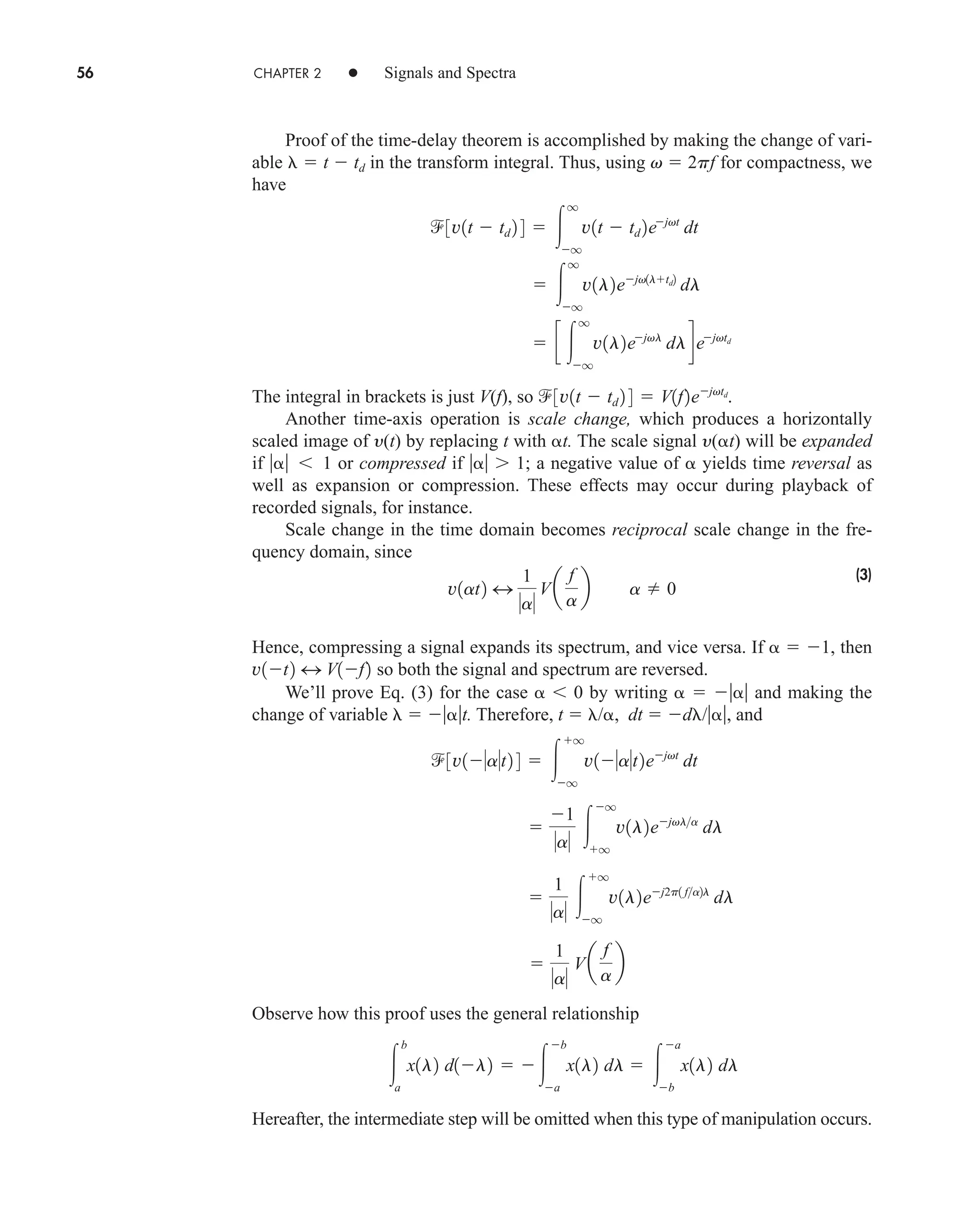
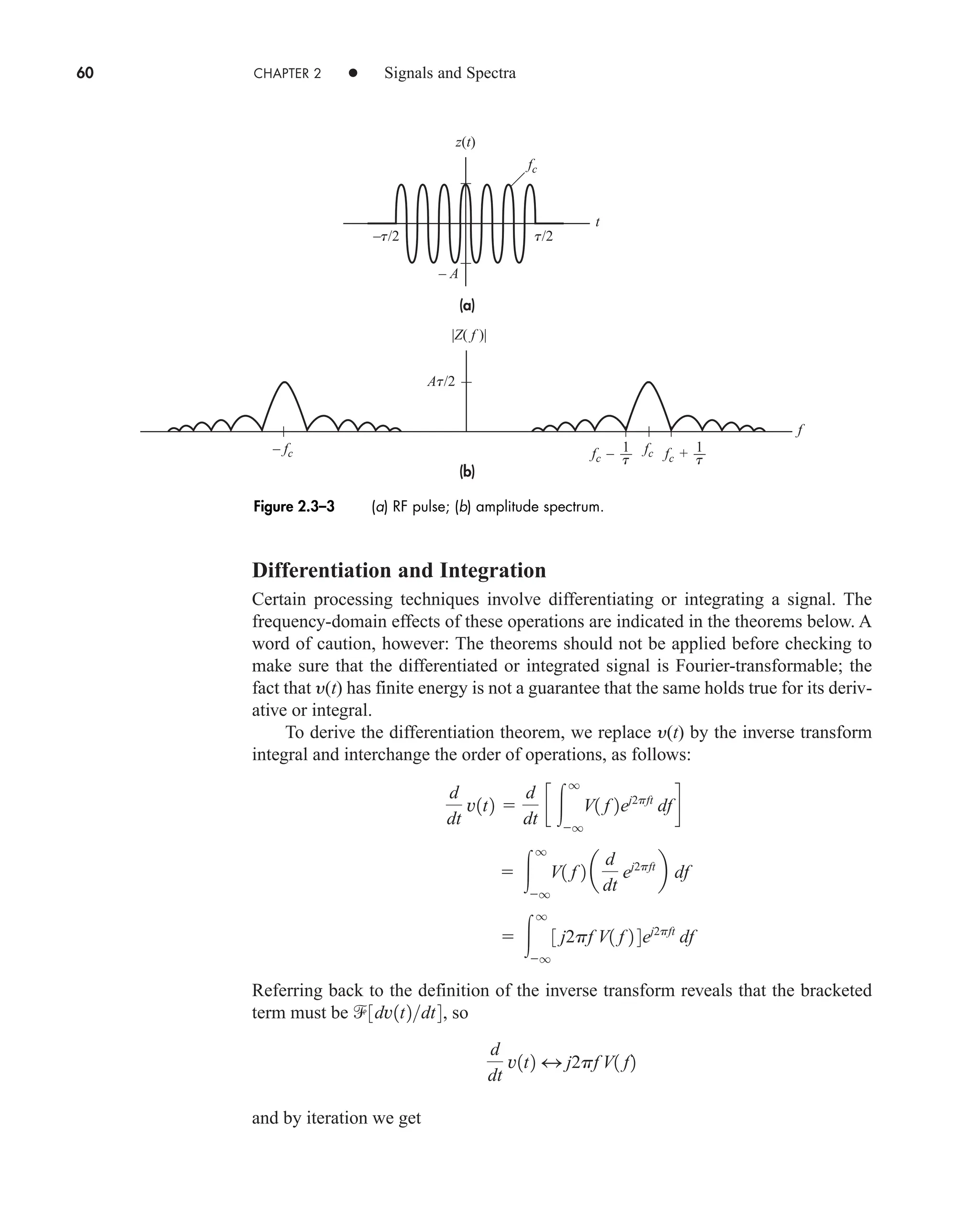
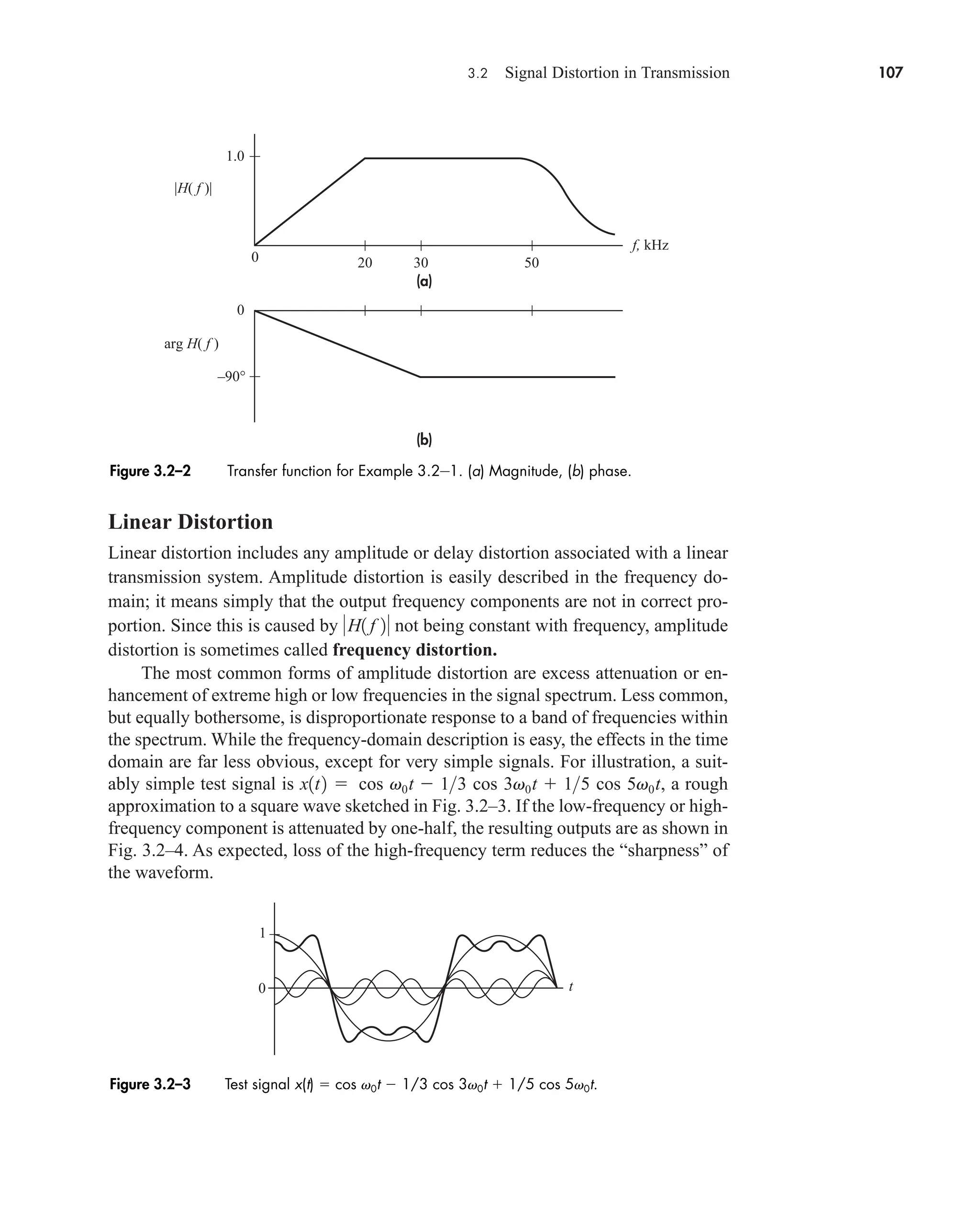
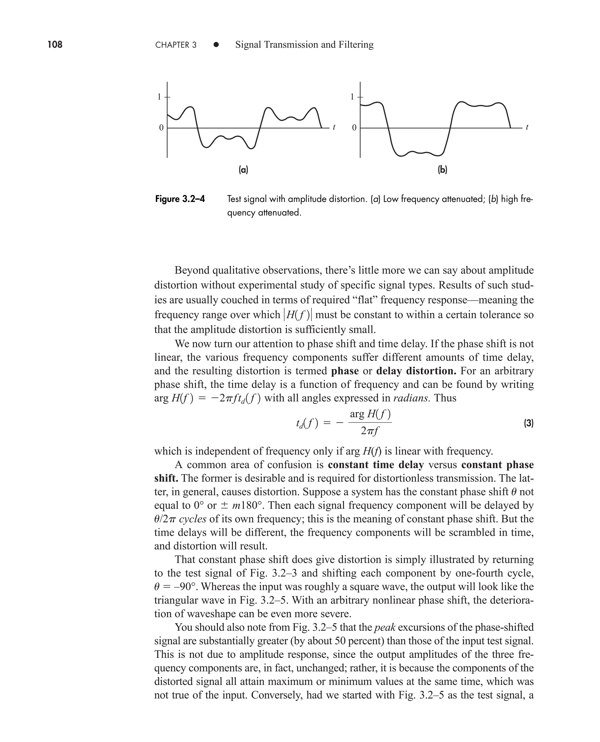
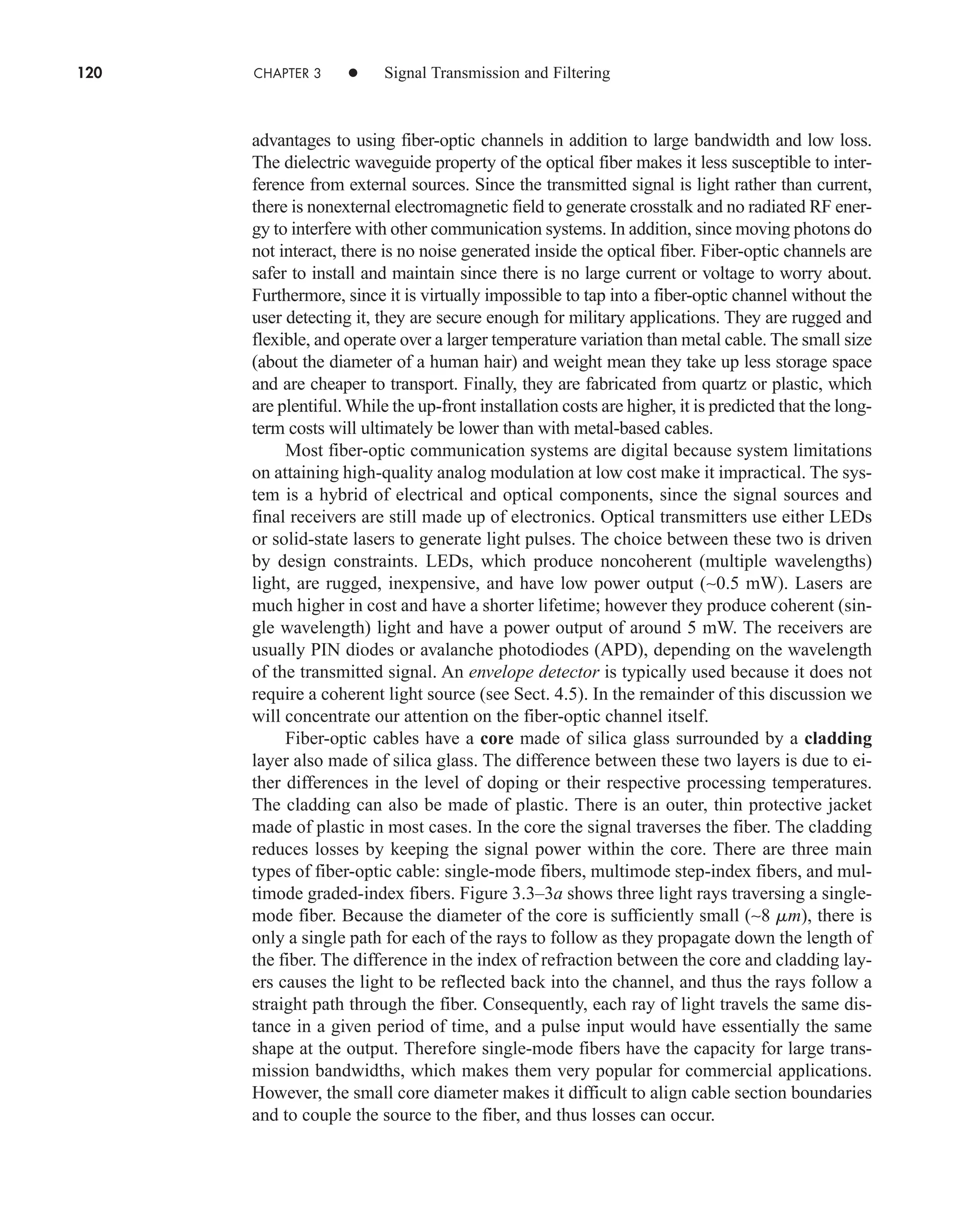
![38 CHAPTER 2 • Signals and Spectra
Multiplying and dividing by t finally gives
(20)
which follows from Eq. (19) with l nf0 t.
The amplitude spectrum obtained from c(nf0) cn Af0 tsinc nf0 is shown
in Fig. 2.1–8a for the case of /T0 f0 1/4. We construct this plot by drawing the
continuous function Af0 tsinc ft as a dashed curve, which becomes the envelope of
the lines. The spectral lines at 4f0, 8f0, and so on, are “missing” since they fall
precisely at multiples of 1/t where the envelope equals zero. The dc component has
amplitude c(0) At/T0 which should be recognized as the average value of v(t) by
inspection of Fig. 2.1–7. Incidentally, t/T0 equals the ratio of “on” time to period,
frequently designated as the duty cycle in pulse electronics work.
cn
At
T0
sinc nf0 t
A
T0
sin pnf0 t
pnf0
A
j2pnf0 T0
1ejpn f0t
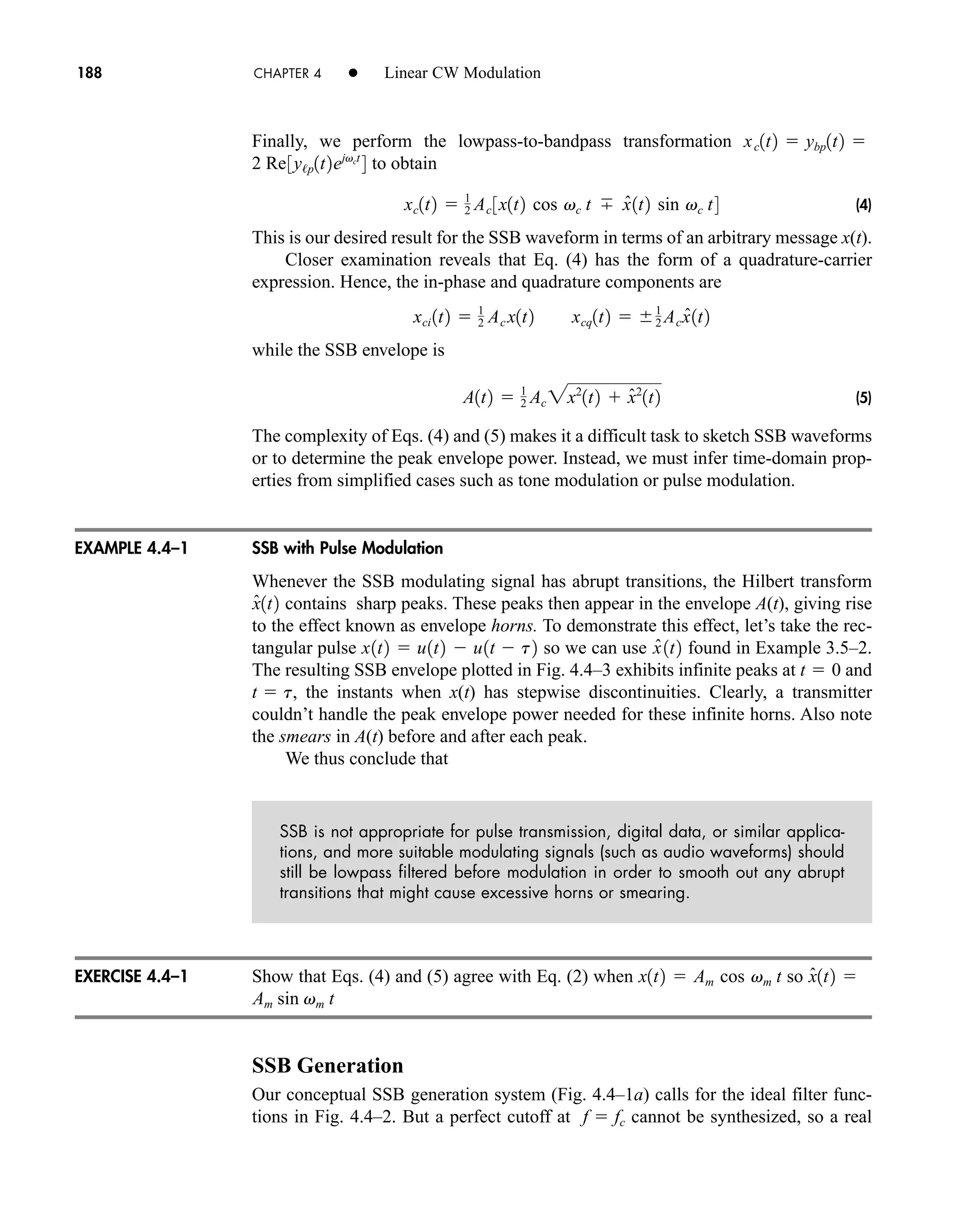
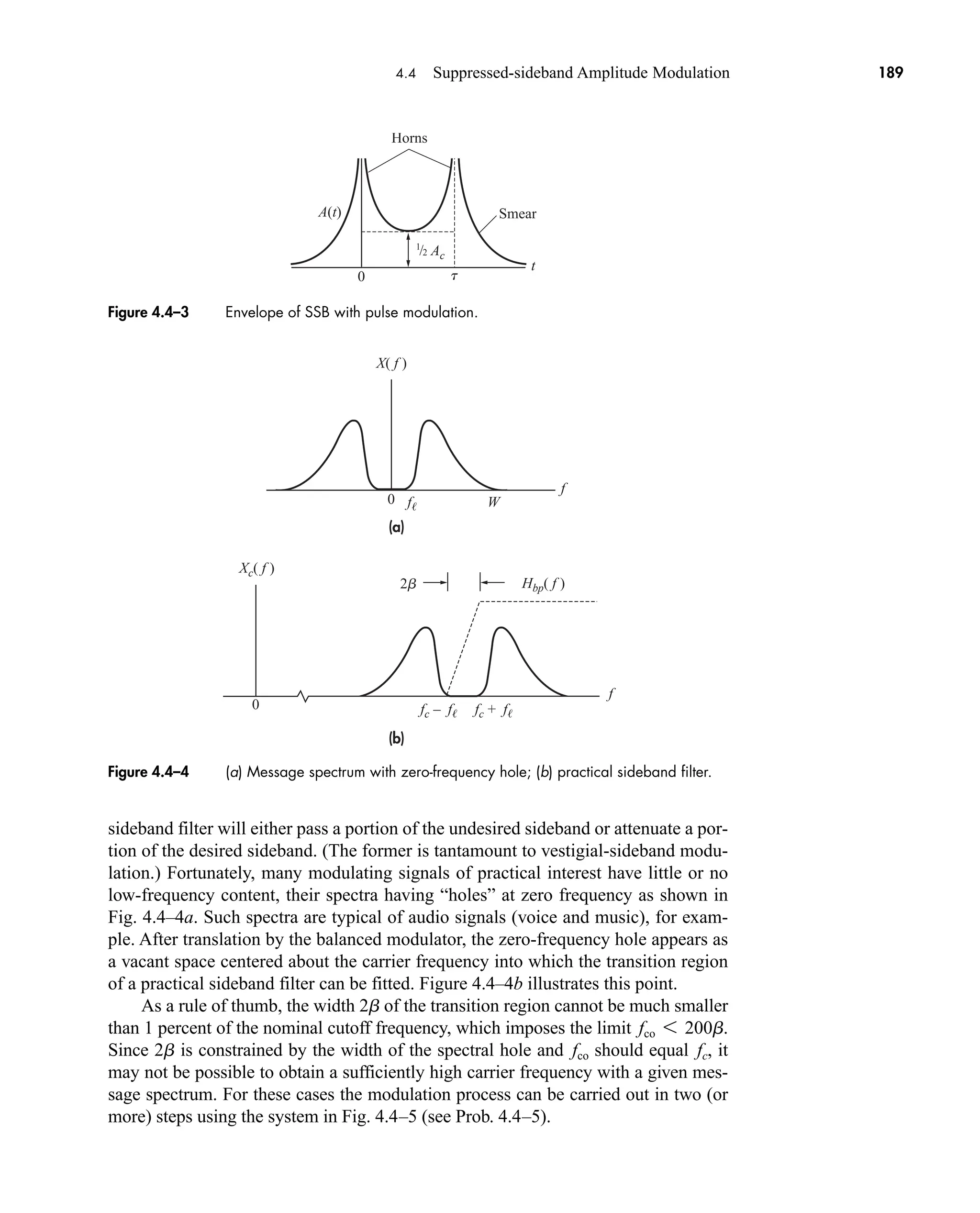
ejpn f0t
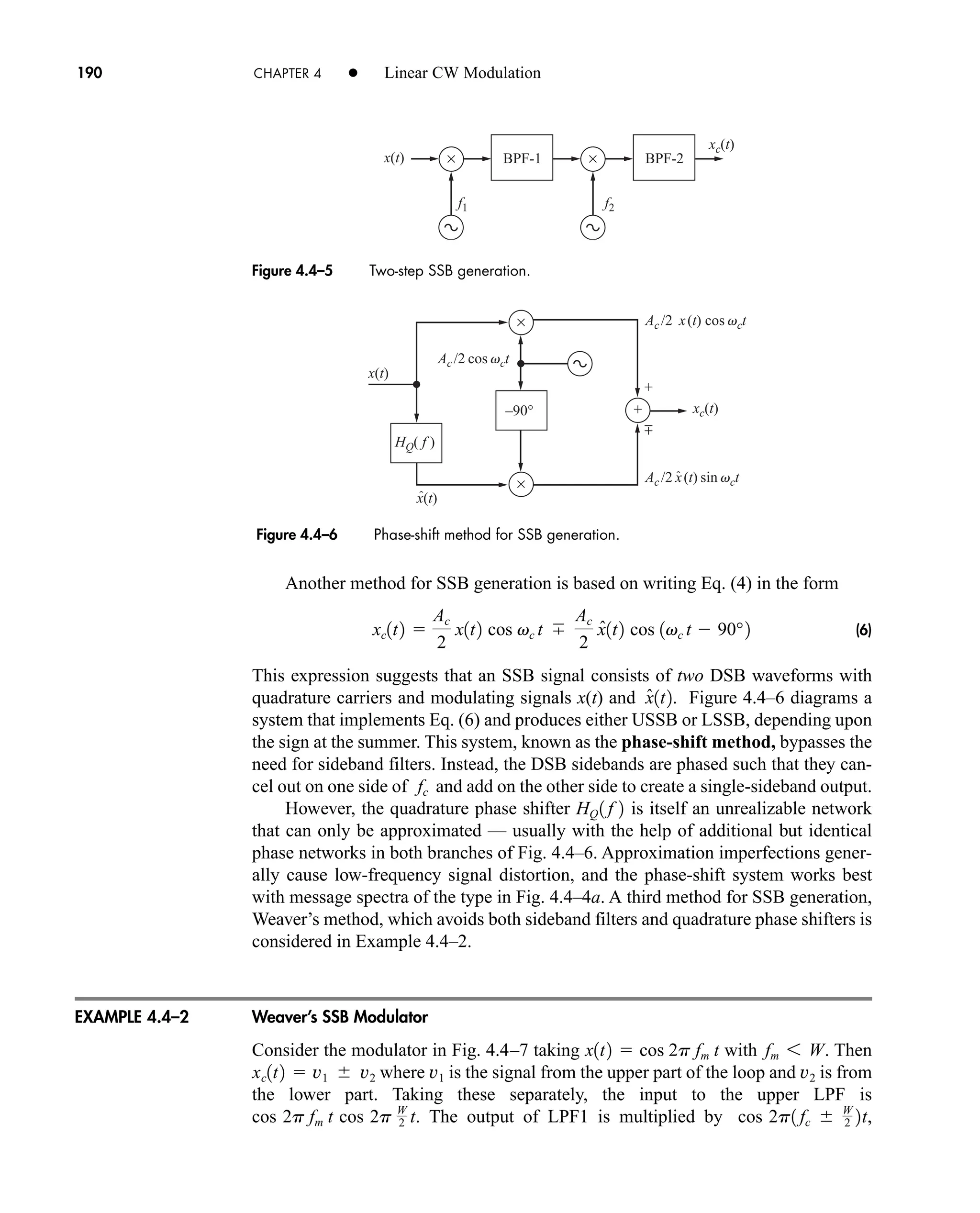
2
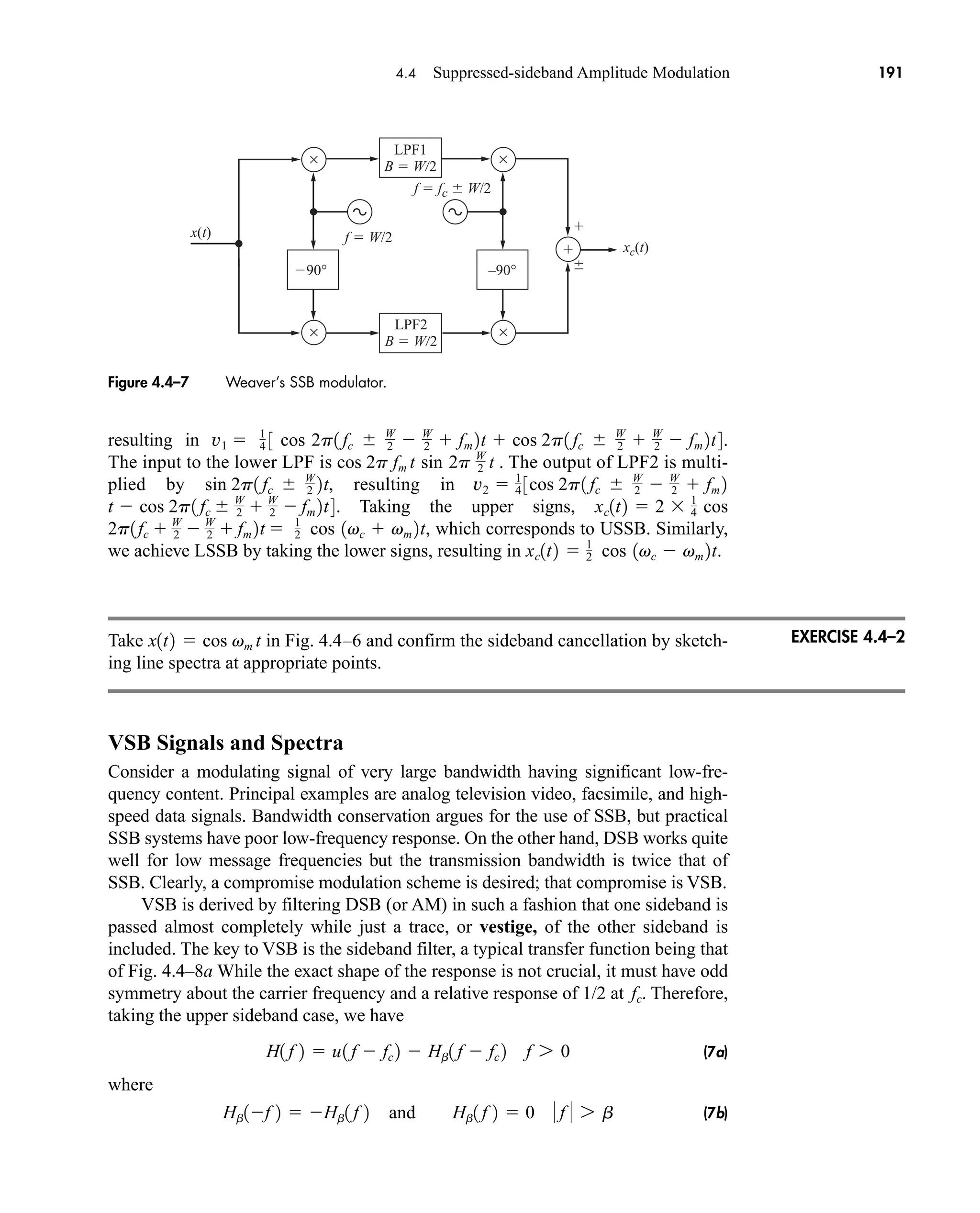
Figure 2.1–7 Rectangular pulse train.
v(t)
0 T0
– T0 –
A
t
t
2
t
2
Figure 2.1–8 Spectrum of rectangular pulse train with fct 1/4. (a) Amplitude; (b) phase.
(a)
(b)
180°
–180°
A f0t
– f0 2 f0
= 4 f0
f0
A f0t|sinc ft|
|c(nf0)|
arg [c( f0)]
f
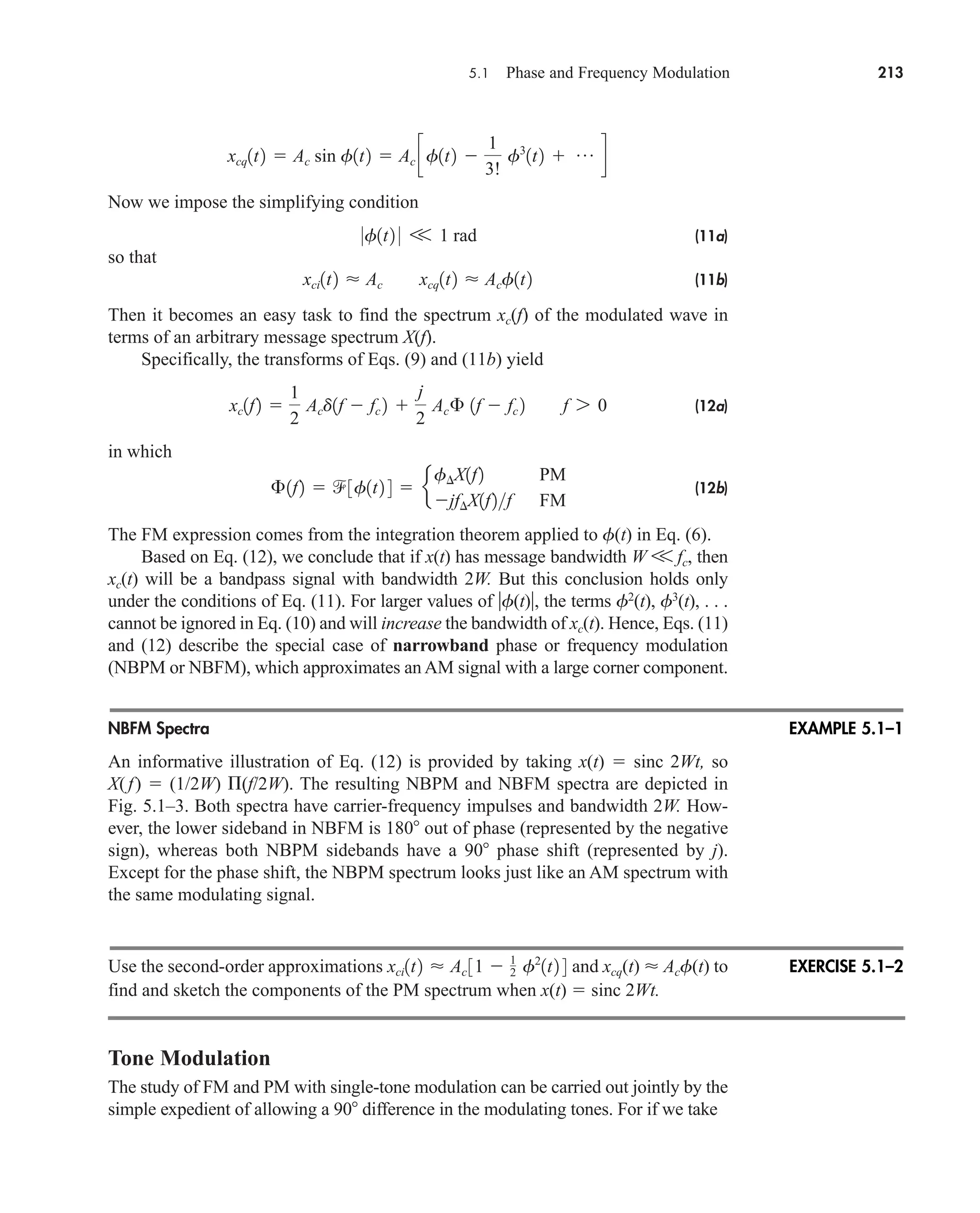
0
0
– t
1
t
1
t
2
t
3
t
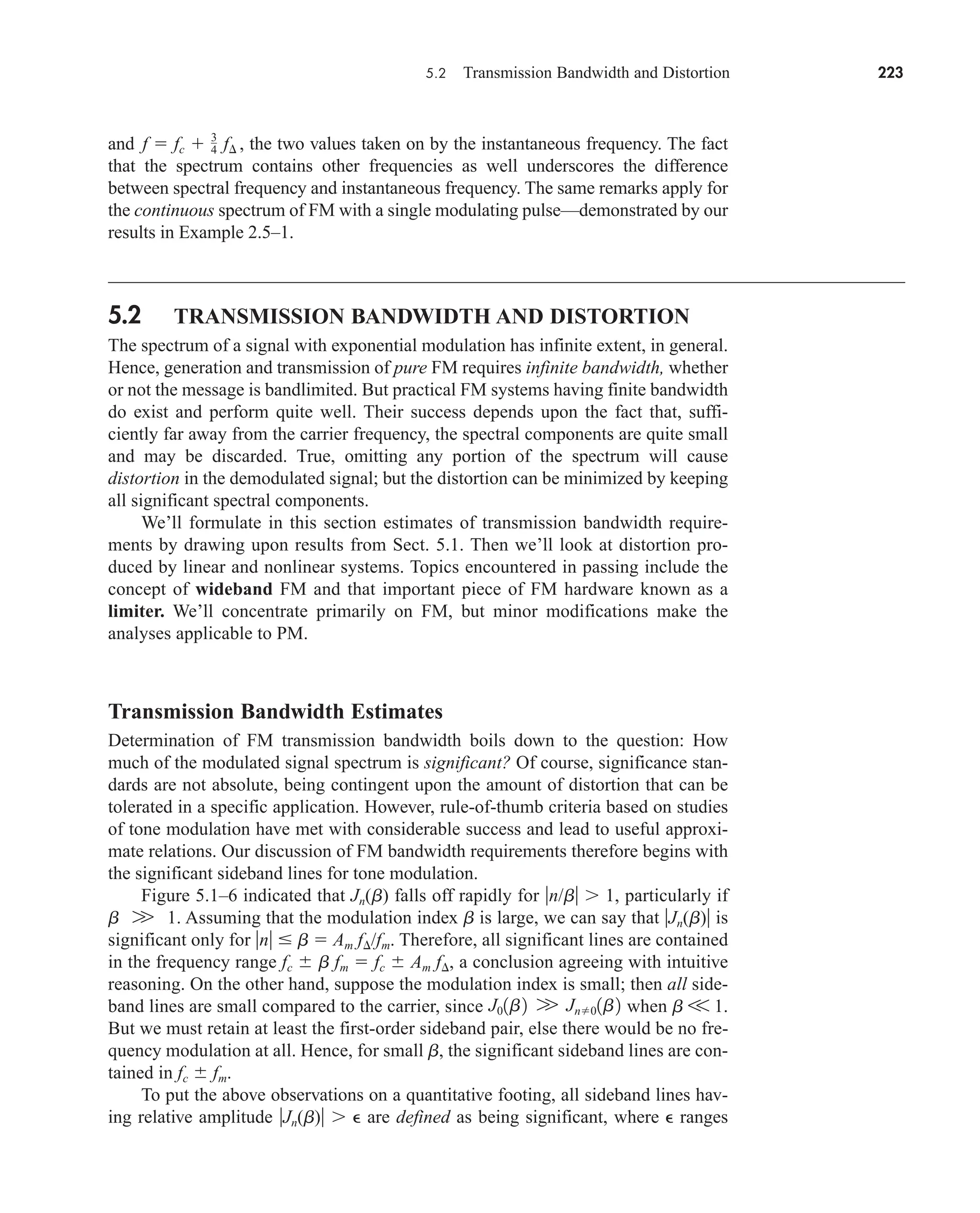
4
t
2
t
1
t
3
t
4
car80407_ch02_027-090.qxd 12/8/08 11:03 PM Page 38](https://image.slidesharecdn.com/communicationsystemsanintro-a-241115060943-61721fa8/75/Communication_Systems__An_Intro_-_A-_Bruce_Carlson_-pdf-60-2048.jpg)
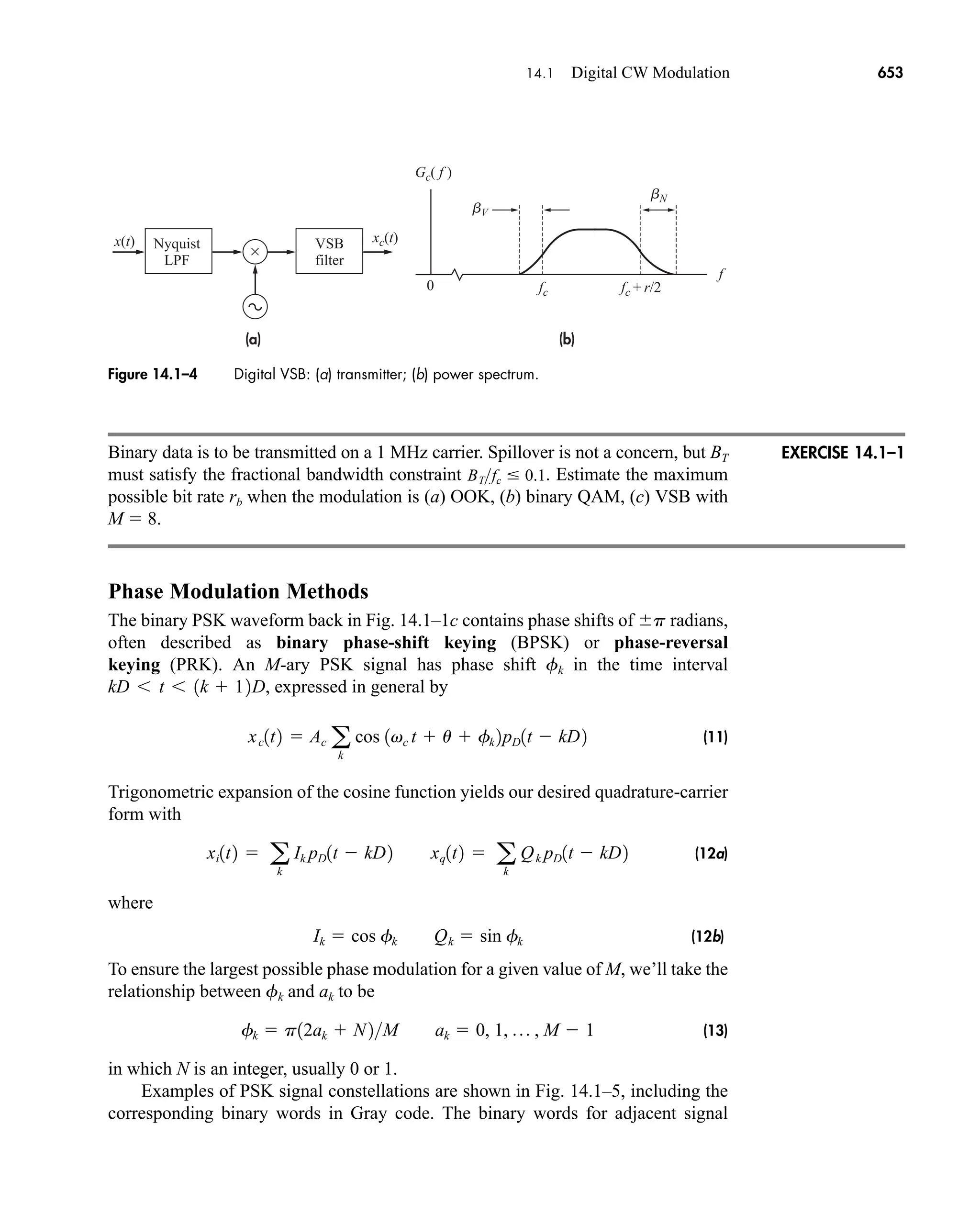
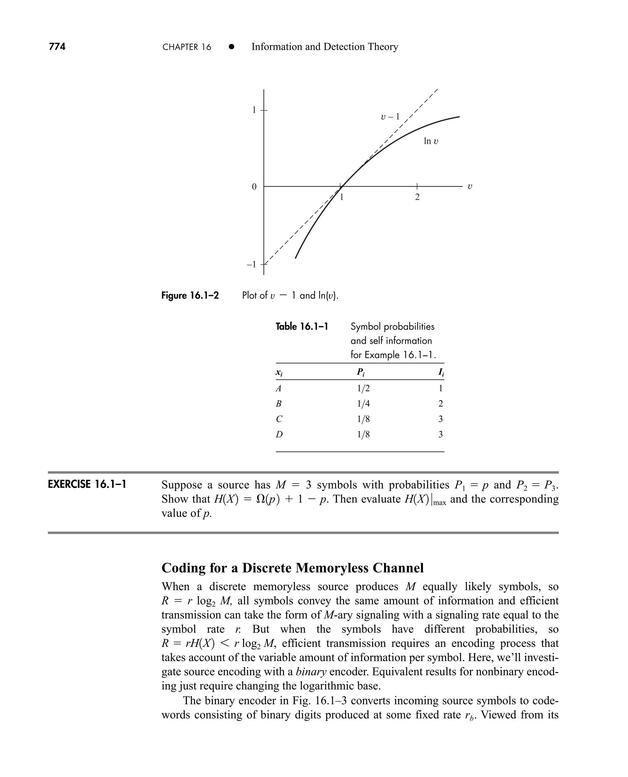
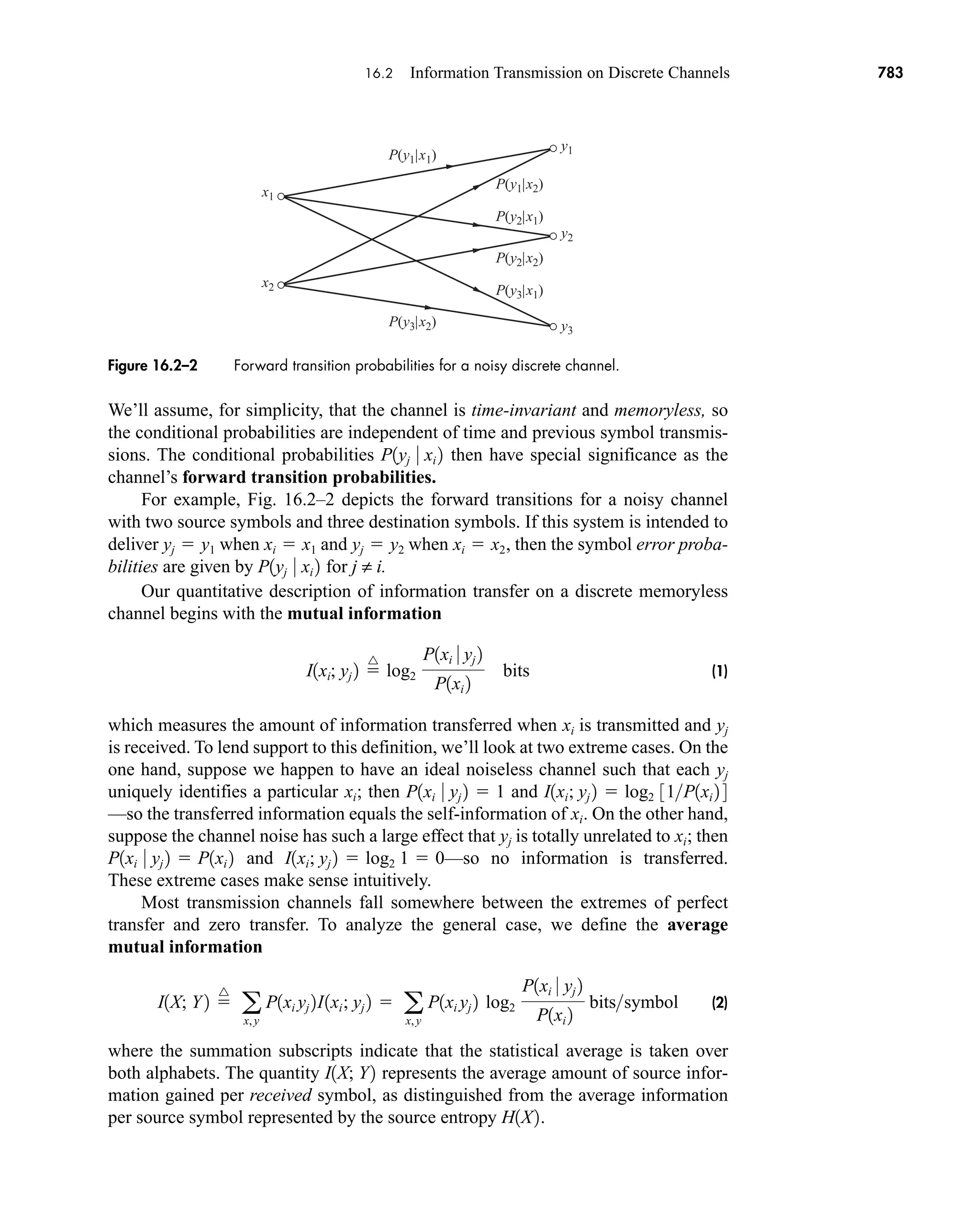
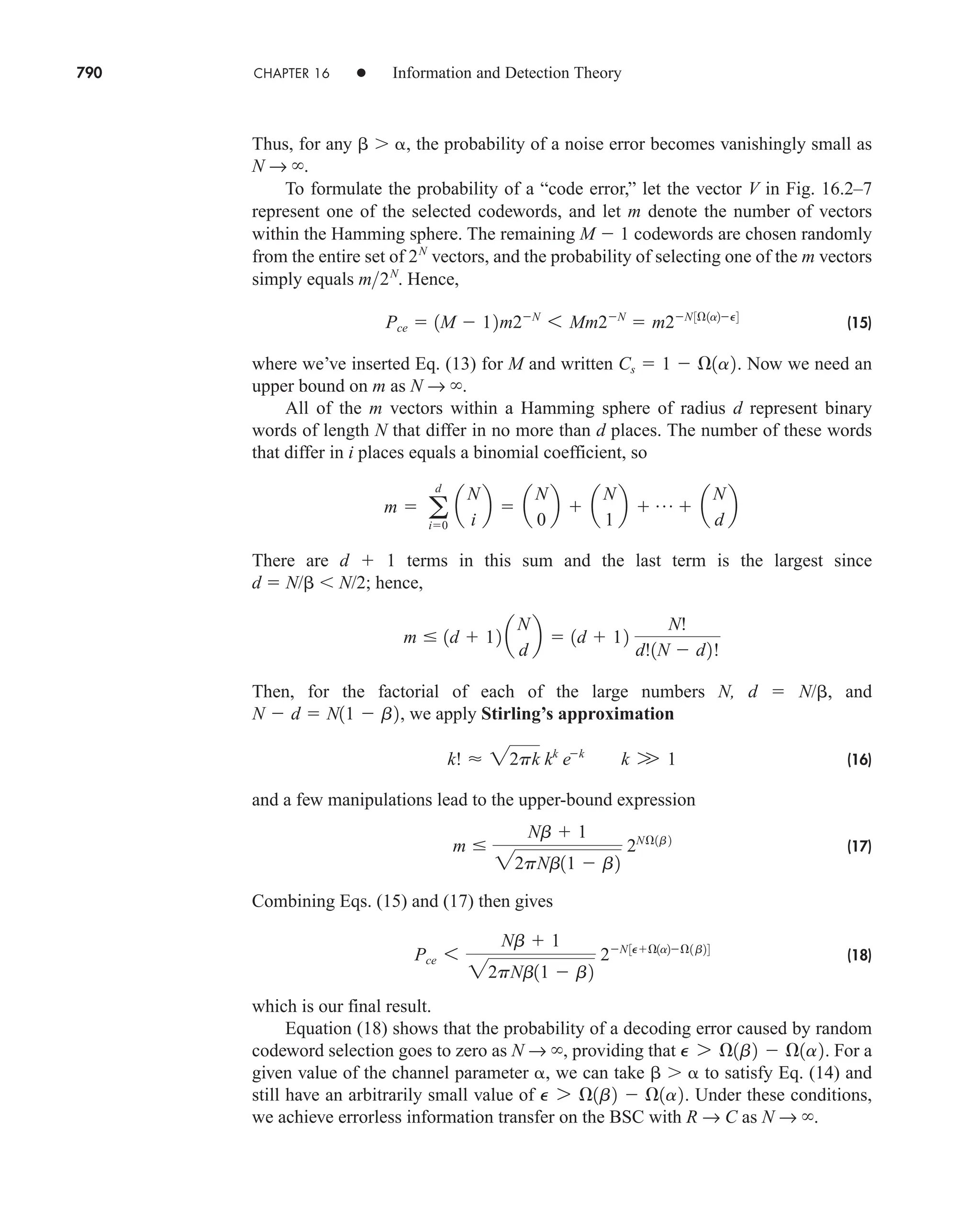
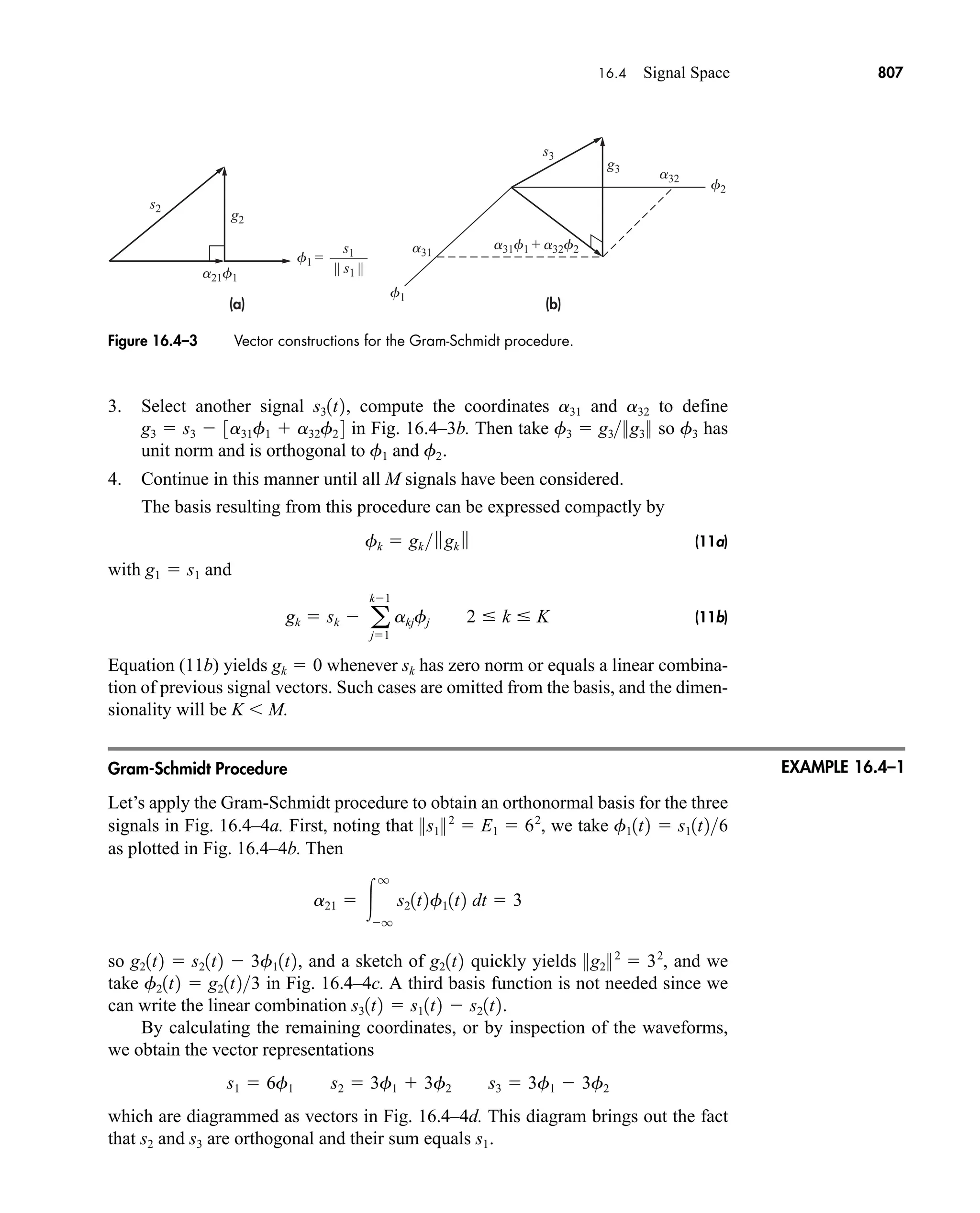
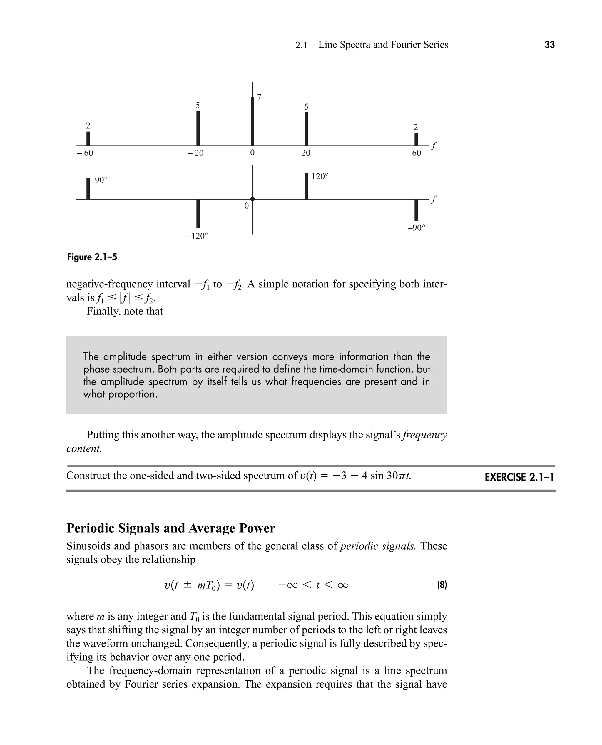
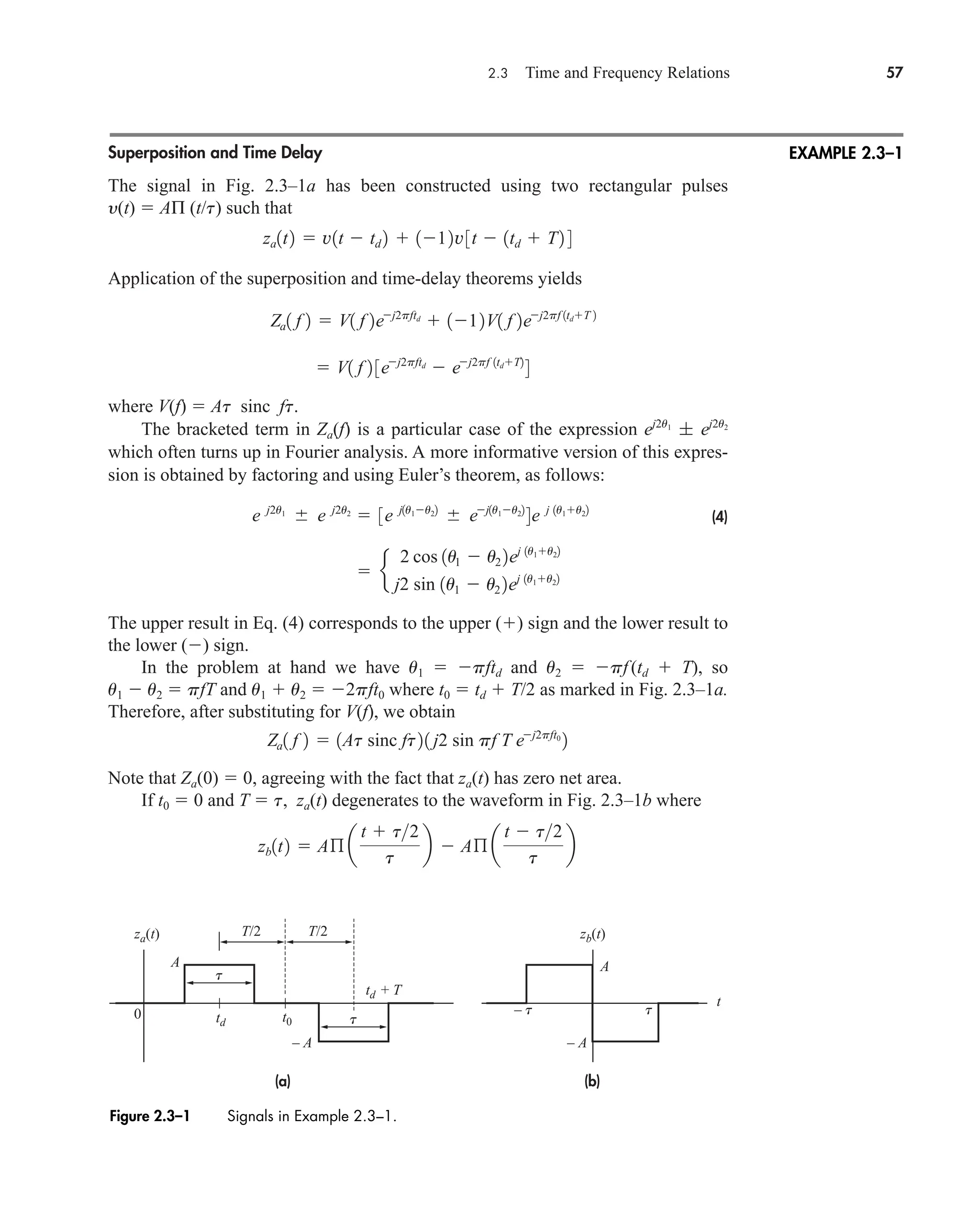
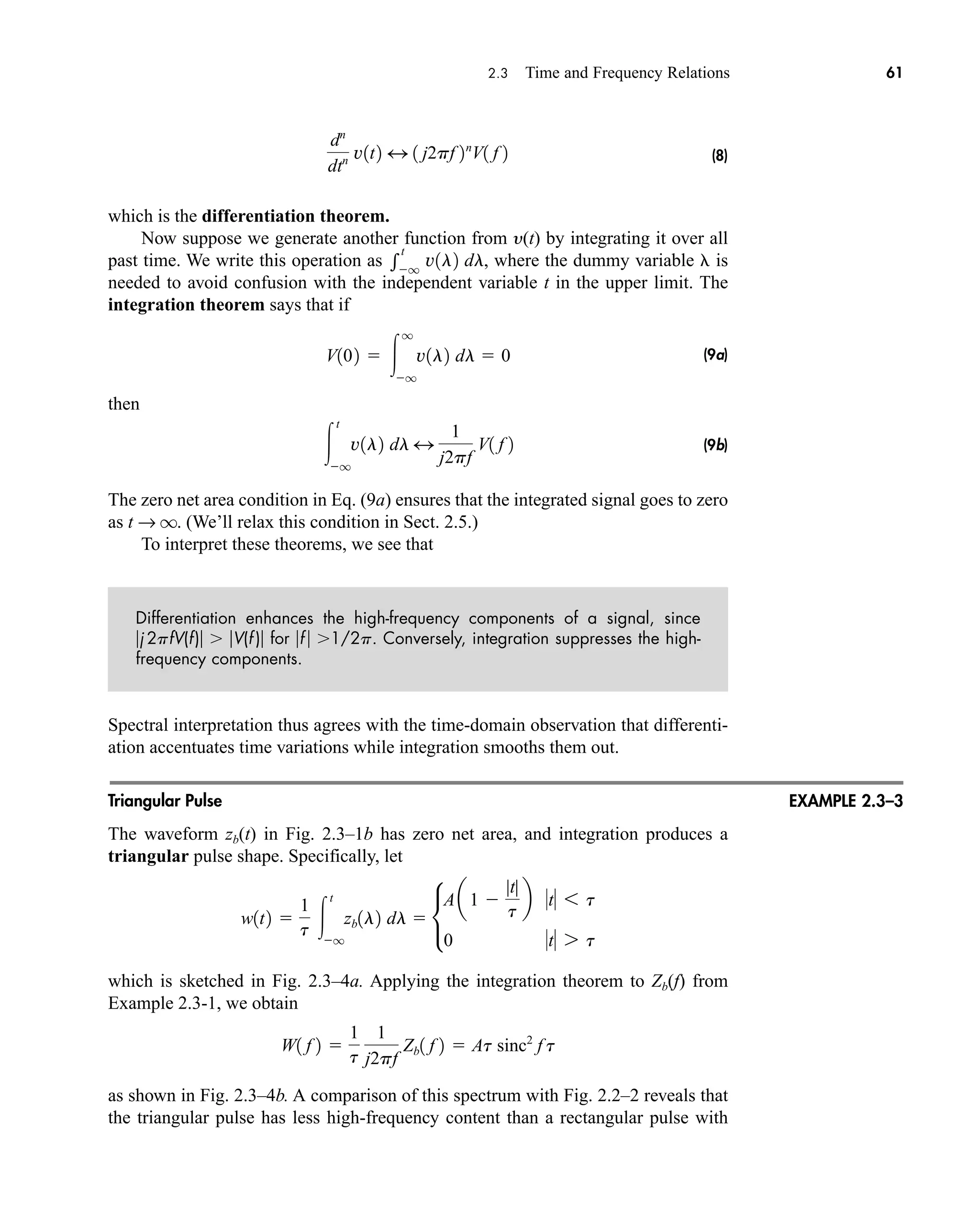
![2.2 Fourier Transforms and Continuous Spectra 53
Although the statement of duality in Eq. (18) seems somewhat abstract, it turns
out to be a handy way of generating new transform pairs without the labor of inte-
gration. The theorem works best when y(t) is real and even so z(t) will also be real
and even, and The following example should clar-
ify the procedure.
Sinc Pulse
A rather strange but important time function in communication theory is the sinc
pulse plotted in Fig. 2.2–5a and defined by
(19a)
We’ll obtain Z(f) by applying duality to the transform pair
Rewriting Eq. (19a) as
brings out the fact that z(t) V(t) with t 2W and B A/2W. Duality then says that
or
(19b)
since the rectangle function has even symmetry.
The plot of Z(f), given in Fig. 2.2–5b, shows that the spectrum of a sinc pulse
equals zero for f W. Thus, the spectrum has clearly defined width W, measured in
terms of positive frequency, and we say that Z(f ) is bandlimited. Note, however,
that the signal z(t) goes on forever and is only asymptotically timelimited.
Find the transform of z(t) B/[1 (2pt)2
] by applying duality to the result of
Exercise 2.2–1.
Z1 f 2
A
2W
ß a
f
2W
b
3z1t2 4 v1f2 Bß1ft2 1A2W2ß1f2W2
z1t2 a
A
2W
b 12W2 sinc t12W2
v1t2 Bß1tt2 V1 f 2 Bt sinc ft
z1t2 A sinc 2Wt
Z1f2 3z1t2 4 v1f2 v1f2.
EXAMPLE 2.2–3
Figure 2.2–5 A sinc pulse and its bandlimited spectrum.
EXERCISE 2.2–3
0 0
f f
W
–W
z(t)
A
Z( f )
–1/2W
A/2W
1/2W
(b)
(a)
car80407_ch02_027-090.qxd 12/8/08 11:03 PM Page 53](https://image.slidesharecdn.com/communicationsystemsanintro-a-241115060943-61721fa8/75/Communication_Systems__An_Intro_-_A-_Bruce_Carlson_-pdf-75-2048.jpg)
![54 CHAPTER 2 • Signals and Spectra
Transform Calculations
Except in the case of a very simple waveform, brute-force integration should be
viewed as the method of last resort for transform calculations. Other, more practical
methods are discussed here.
When the signal in question is defined mathematically, you should first consult
a table of Fourier transforms to see if the calculation has been done before. Both
columns of the table may be useful, in view of the duality theorem. A table of
Laplace transforms also has some value, as mentioned in conjunction with Eq. (14).
Besides duality, there are several additional transform theorems covered in
Sect. 2.3. These theorems often help you decompose a complicated waveform into
simpler parts whose transforms are known. Along this same line, you may find it
expedient to approximate a waveform in terms of idealized signal models. Suppose
z̃(t) approximates z(t) and magnitude-squared error z(t) z̃(t)2
is a small quantity. If
Z(f) [z(t)] and
~
Z(f ) [z̃(t)] then
(20)
which follows from Rayleigh’s theorem with v(t) z(t) z̃(t). Thus, the integrated
approximation error has the same value in the time and frequency domains.
The above methods are easily modified for the calculation of Fourier series
coefficients. Specifically, let v(t) be a periodic signal and let z(t) v(t)Π (t/T0), a
nonperiodic signal consisting of one period of v(t). If you can obtain
(21a)
then, from Eq. (14), Sect. 2.1, the coefficients of v(t) are given by
(21b)
This relationship facilitates the application of transform theorems to Fourier series
calculations.
Finally, if the signal is expressed in numerical form as a set of samples, its trans-
form, as we will see in Sect. 2.6, can be found via numerical calculations. For this
purpose the Discrete Fourier Transform (DFT) and its faster version, the Fast Fourier
Transform is used.
2.3 TIME AND FREQUENCY RELATIONS
Rayleigh’s theorem and the duality theorem in the previous section helped us draw
useful conclusions about the frequency-domain representation of energy signals.
Now we’ll look at some of the many other theorems associated with Fourier trans-
forms. They are included not just as manipulation exercises but for two very practical
reasons. First, the theorems are invaluable when interpreting spectra, for they express
cn
1
T0
Z1nf0 2
Z1 f 2 3v1t2ß1tT0 2 4
q
q
0 Z1 f 2 Z
1 f 2 02
df
q
q
0z1t2 z
1t2 02
dt
car80407_ch02_027-090.qxd 12/15/08 9:29 PM Page 54](https://image.slidesharecdn.com/communicationsystemsanintro-a-241115060943-61721fa8/75/Communication_Systems__An_Intro_-_A-_Bruce_Carlson_-pdf-76-2048.jpg)
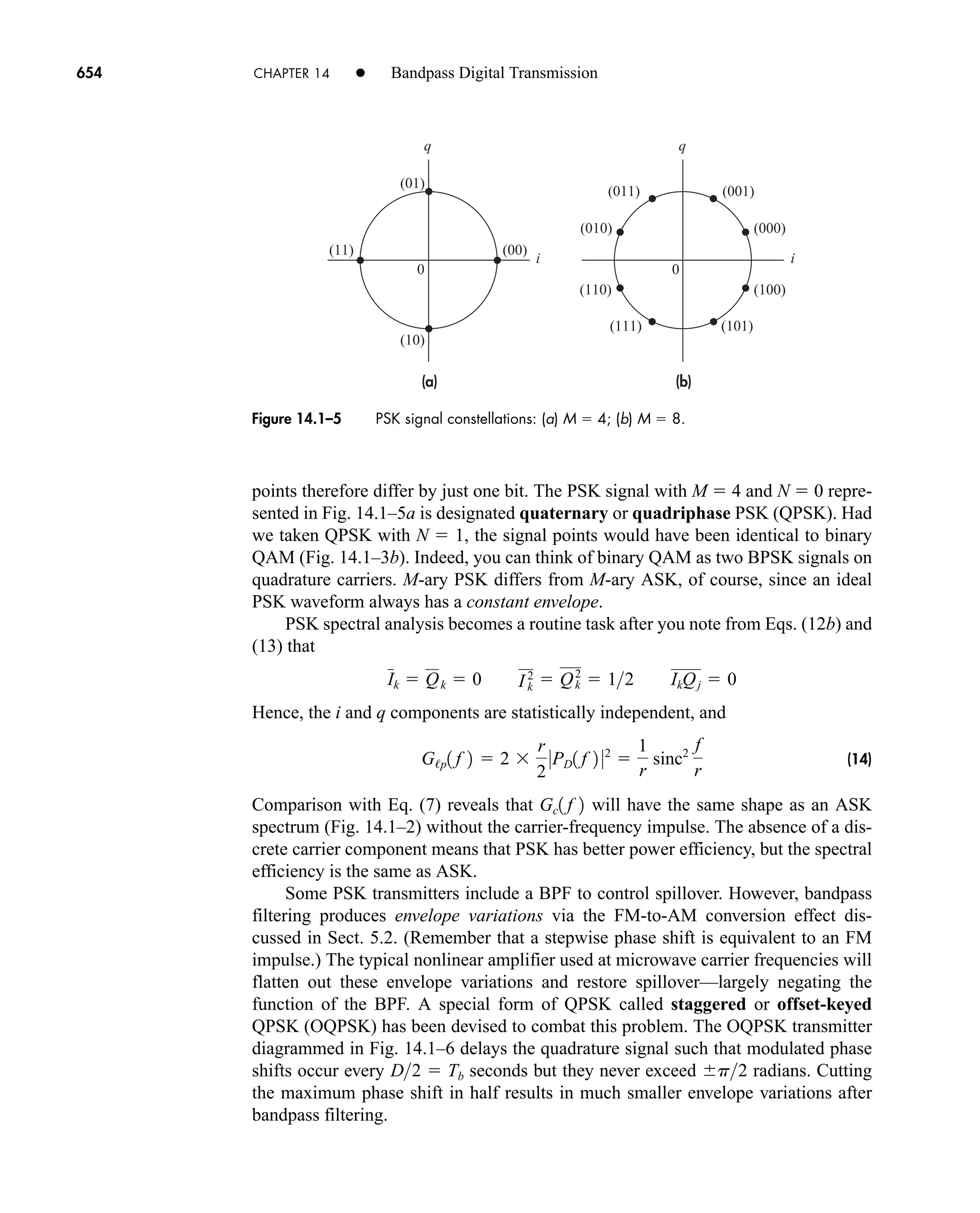
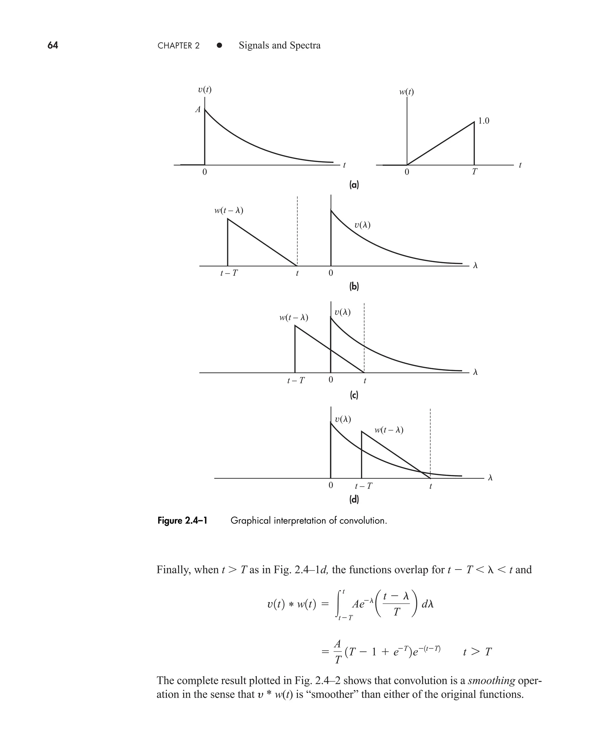
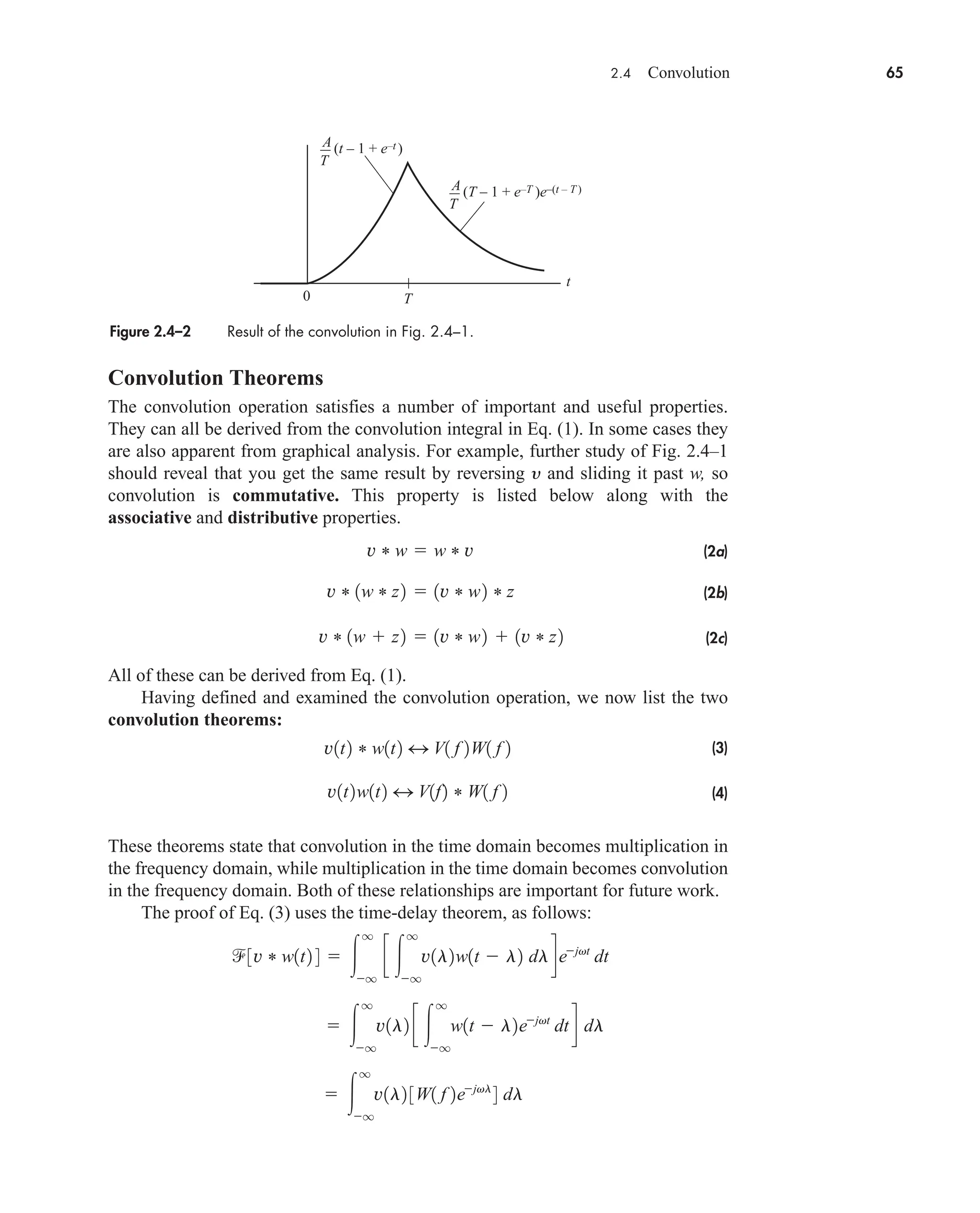
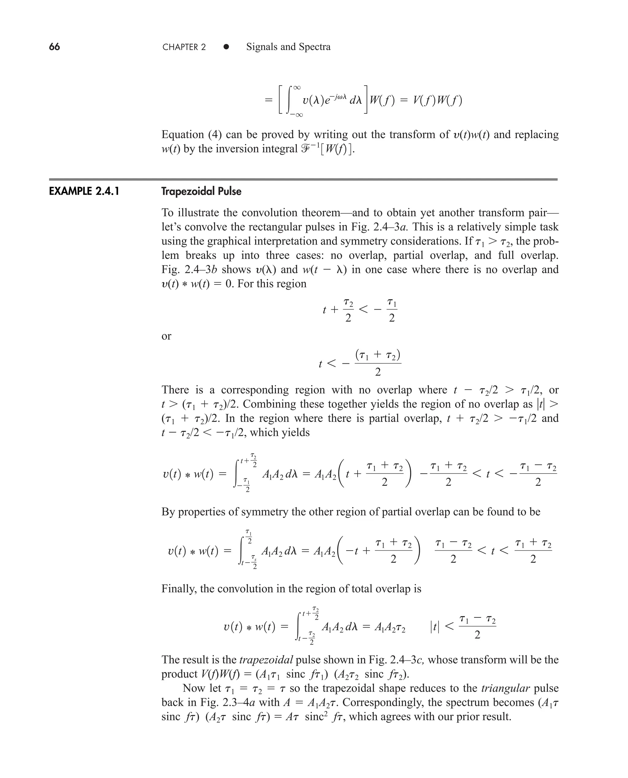
![2.4 Convolution 63
Convolution Integral
The convolution of two functions of the same variable, say y(t) and w(t), is defined by
(1)
The notation y(t) * w(t) merely stands for the operation on the right-hand side of
Eq. (1) and the asterisk (*) has nothing to do with complex conjugation. Equation (1)
is the convolution integral, often denoted y * w when the independent variable is
unambiguous. At other times the notation [y(t)] * [w(t)] is necessary for clarity. Note
carefully that the independent variable here is t, the same as the independent variable
of the functions being convolved; the integration is always performed with respect to a
dummy variable (such as ), and t is a constant insofar as the integration is concerned.
Calculating y(t) * w(t) is no more difficult than ordinary integration when the
two functions are continuous for all t. Often, however, one or both of the functions is
defined in a piecewise fashion, and the graphical interpretation of convolution
becomes especially helpful.
By way of illustration, take the functions in Fig. 2.4–1a where
For the integrand in Eq. (1), y( ) has the same shape as y(t) and
But obtaining the picture of w(t ) as a function of requires two steps: First, we
reverse w(t) in time and replace t with to get w( ); second, we shift w( ) to the
right by t units to get w[( t)] w(t ) for a given value of t. Fig. 2.4–1b
shows y( ) and w(t ) with t 0. The value of t always equals the distance from
the origin of y( ) to the shifted origin of w( ) indicated by the dashed line.
As y(t) * w(t) is evaluated for q t q, w(t ) slides from left to right
with respect to y( ), so the convolution integrand changes with t. Specifically, we
see in Fig. 2.4–1b that the functions don’t overlap when t 0; hence, the integrand
equals zero and
When 0 t T as in Fig. 2.4–1c, the functions overlap for 0 t, so t
becomes the upper limit of integration and
A
T
1t 1 et
2 0 6 t 6 T
v1t2 * w1t2
t
0
Ael
a
t l
T
b dl
v1t2 * w1t2 0 t 6 0
w1t l2
t l
T
0 6 t l 6 T
w1t2 tT 0 6 t 6 T
v1t2 Aet
0 6 t 6 q
v1t2 * w1t2
^
q
q
v1l2w1t l2 dl
car80407_ch02_027-090.qxd 12/8/08 11:03 PM Page 63](https://image.slidesharecdn.com/communicationsystemsanintro-a-241115060943-61721fa8/75/Communication_Systems__An_Intro_-_A-_Bruce_Carlson_-pdf-85-2048.jpg)
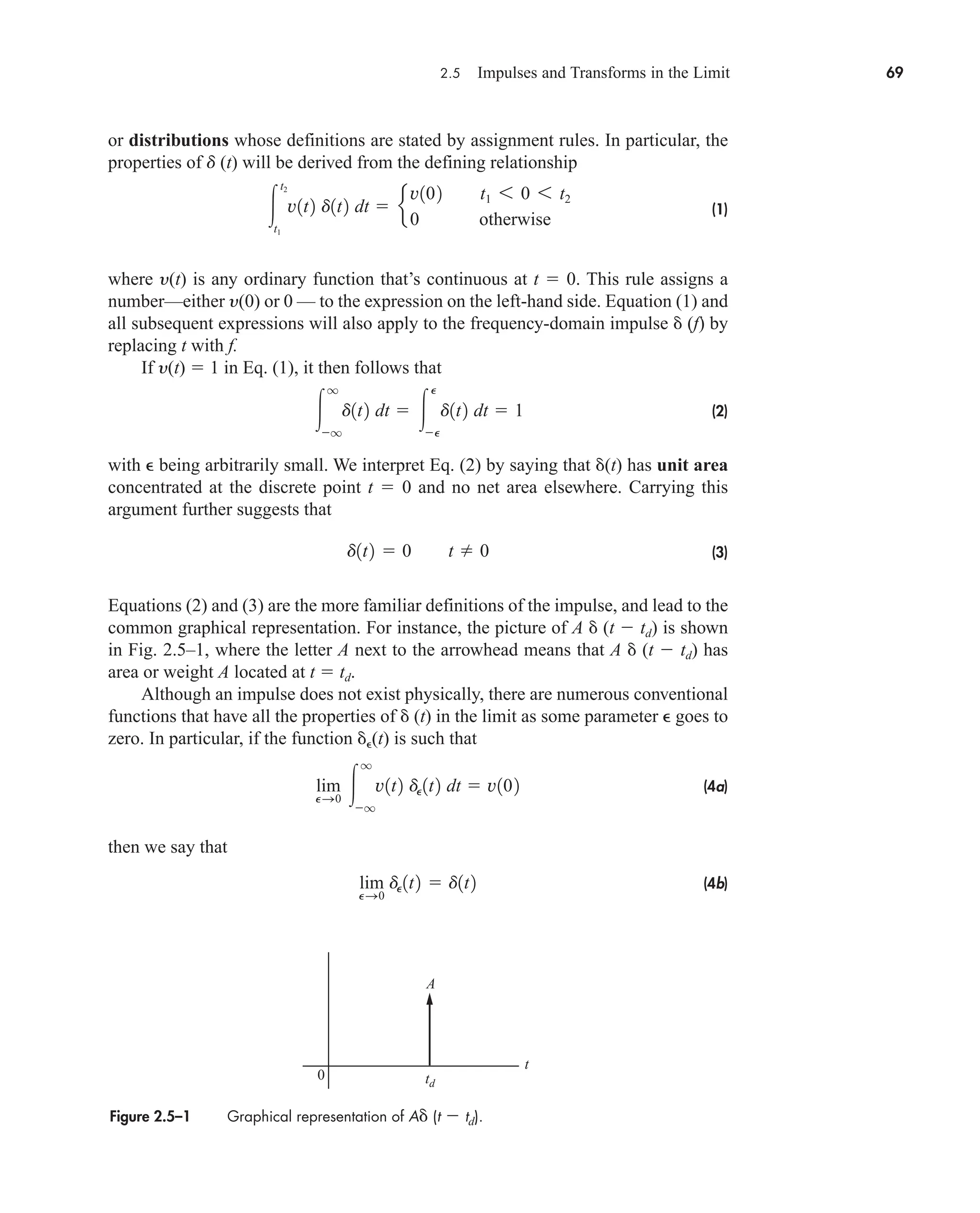
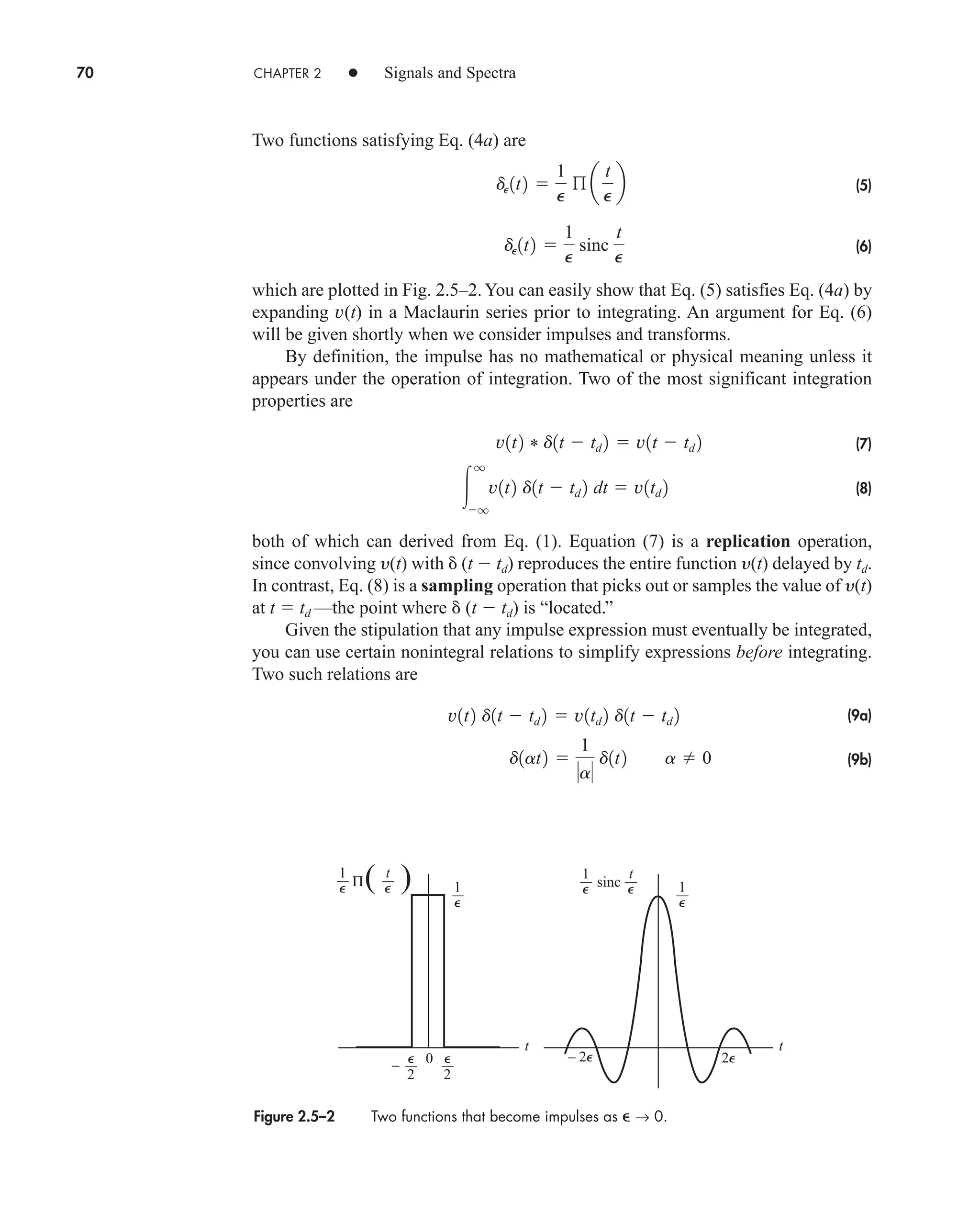
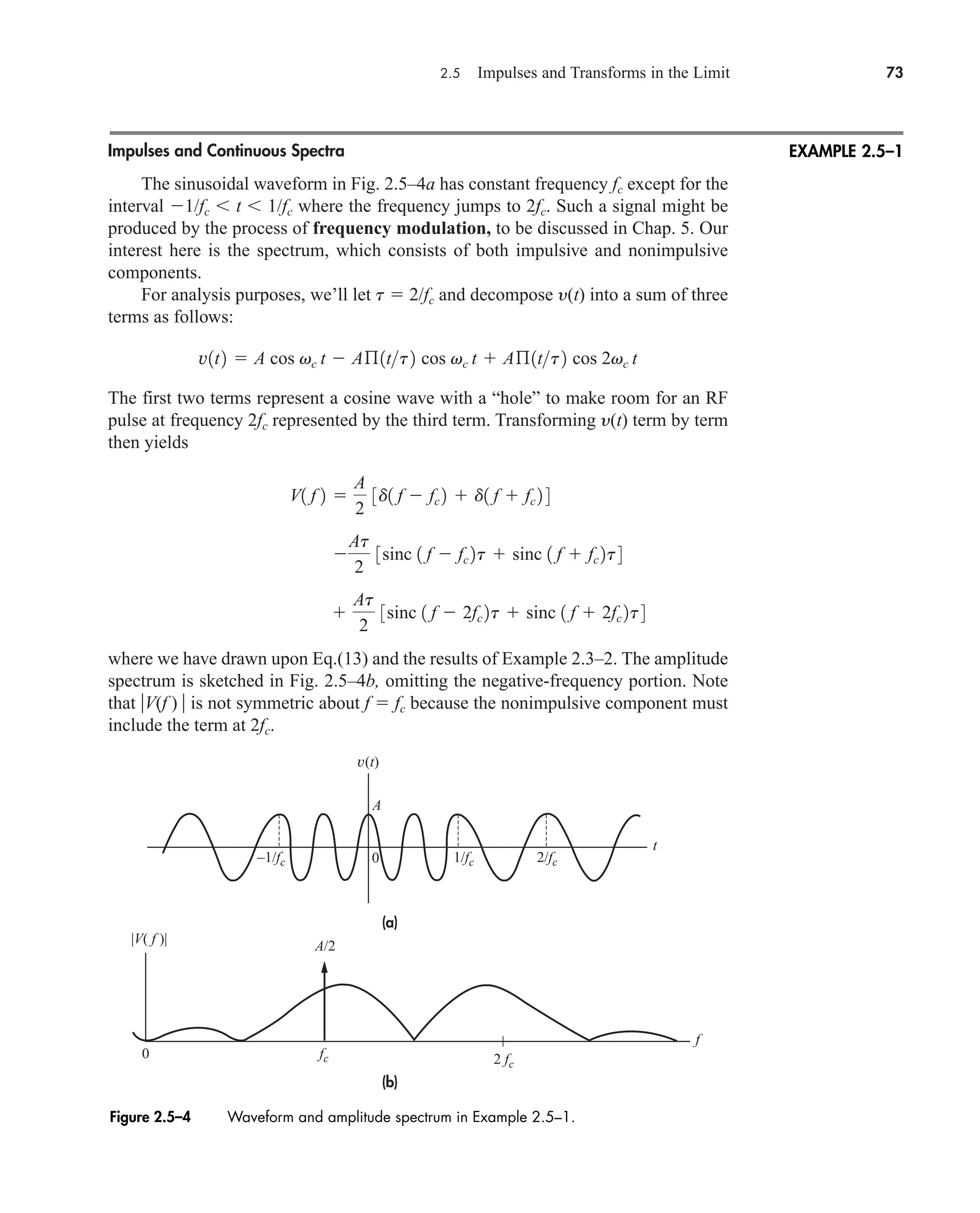
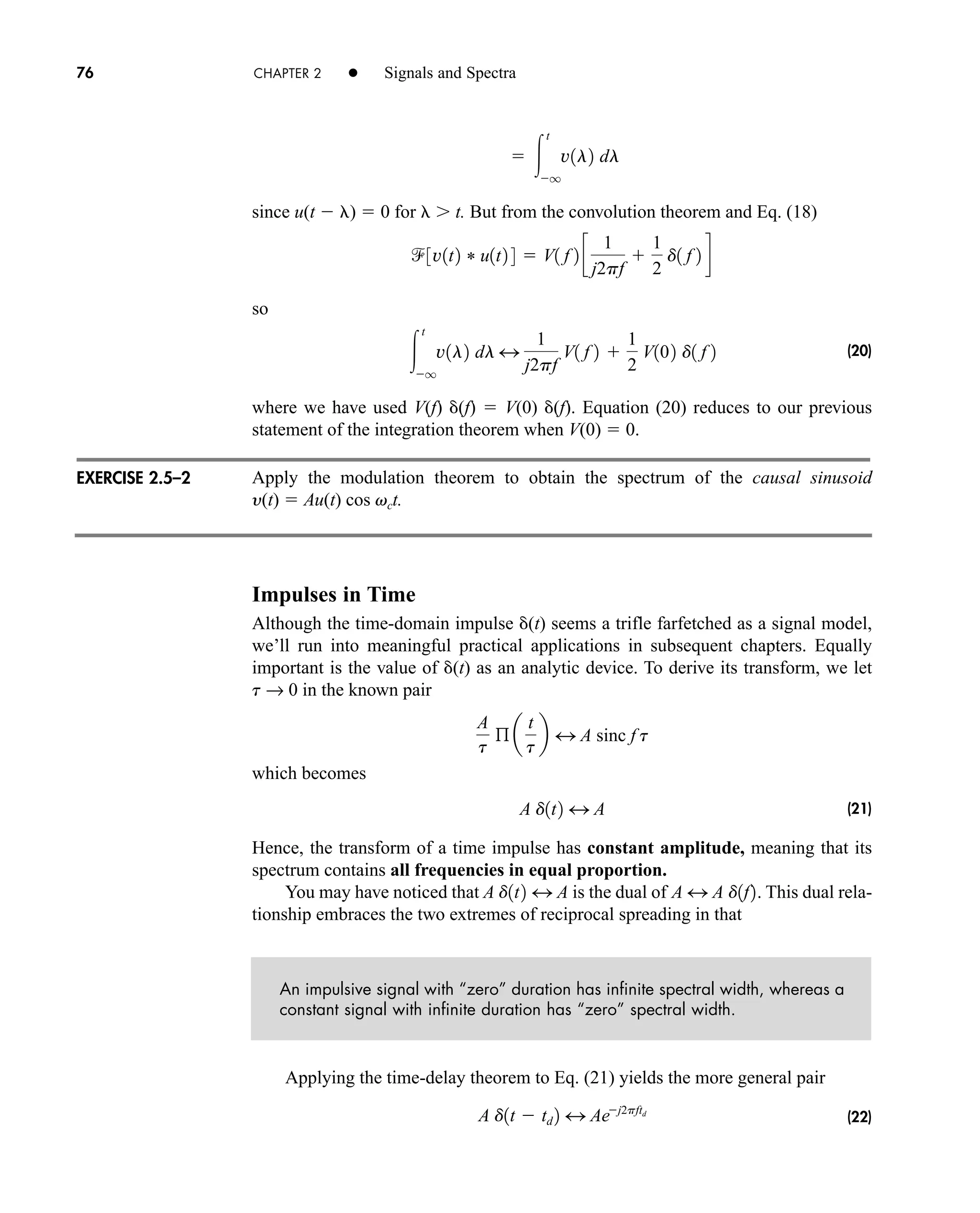
![2.5 Impulses and Transforms in the Limit 77
It’s a simple matter to confirm the direct transform relationship [Ad(t td)]
consistency therefore requires that A d(t td), which
leads to a significant integral expression for the unit impulse. Specifically, since
we conclude that
(23)
Thus, the integral on the left side may be evaluated in the limiting form of the unit
impulse—a result we’ll put immediately to work in a proof of the Fourier integral
theorem.
Let y(t) be a continuous time function with a well-defined transform
Our task is to show that the inverse transform does, indeed, equal
y(t). From the definitions of the direct and inverse transforms we can write
But the bracketed integral equals (t ), from Eq. (23), so
(24)
Therefore equals y(t), in the same sense that y(t) * (t) y(t). A more
rigorous proof, including Gibbs’s phenomena at points of discontinuity, is given by
Papoulis (1962, Chap. 2).
Lastly, we relate the unit impulse to the unit step by means of the integral
(25)
Differentiating both sides then yields
(26)
which provides another interpretation of the impulse in terms of the derivative of a
step discontinuity.
Equations (26) and (22), coupled with the differentiation theorem, expedite cer-
tain transform calculations and help us predict a signal’s high-frequency spectral
d1t td 2
d
dt
u1t td 2
u1t td 2
t
q
d1l td 2 dl e
1 t 7 td
0 t 6 td
1
3V1f2 4
1
3V1 f 2 4
q
q
v1l2 d1t l2 dl v1t2 * d1t2
q
q
v1l2 c
q
q
ej2p1tl2 f
df d dl
1
3V1 f 2 4
q
q
c
q
q
v1l2ej2pfl
dldej2pft
df
V1f2 3v1t2 4.
q
q
ej2pf 1ttd2
df d1t td 2
1
3ej2pftd
4
q
q
ej2pftd
ej2pft
df
1
3Aej2pftd
4
Aej2pftd
;
car80407_ch02_027-090.qxd 12/8/08 11:04 PM Page 77](https://image.slidesharecdn.com/communicationsystemsanintro-a-241115060943-61721fa8/75/Communication_Systems__An_Intro_-_A-_Bruce_Carlson_-pdf-99-2048.jpg)
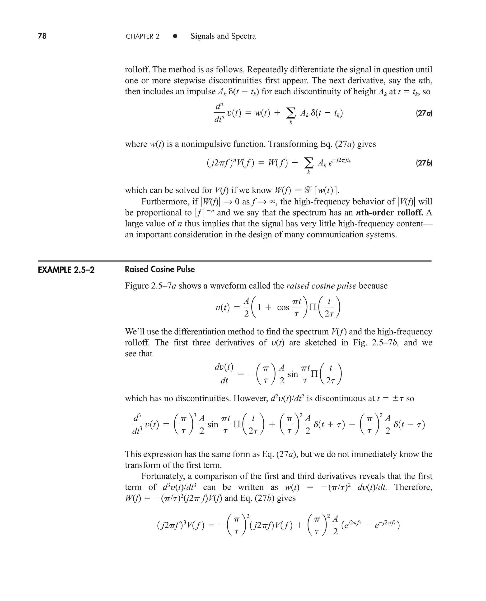
![80 CHAPTER 2 • Signals and Spectra
Let y(t) (2At/t)Π (t/t). Sketch dy(t)/dt and use Eq. (27) to find V(f).
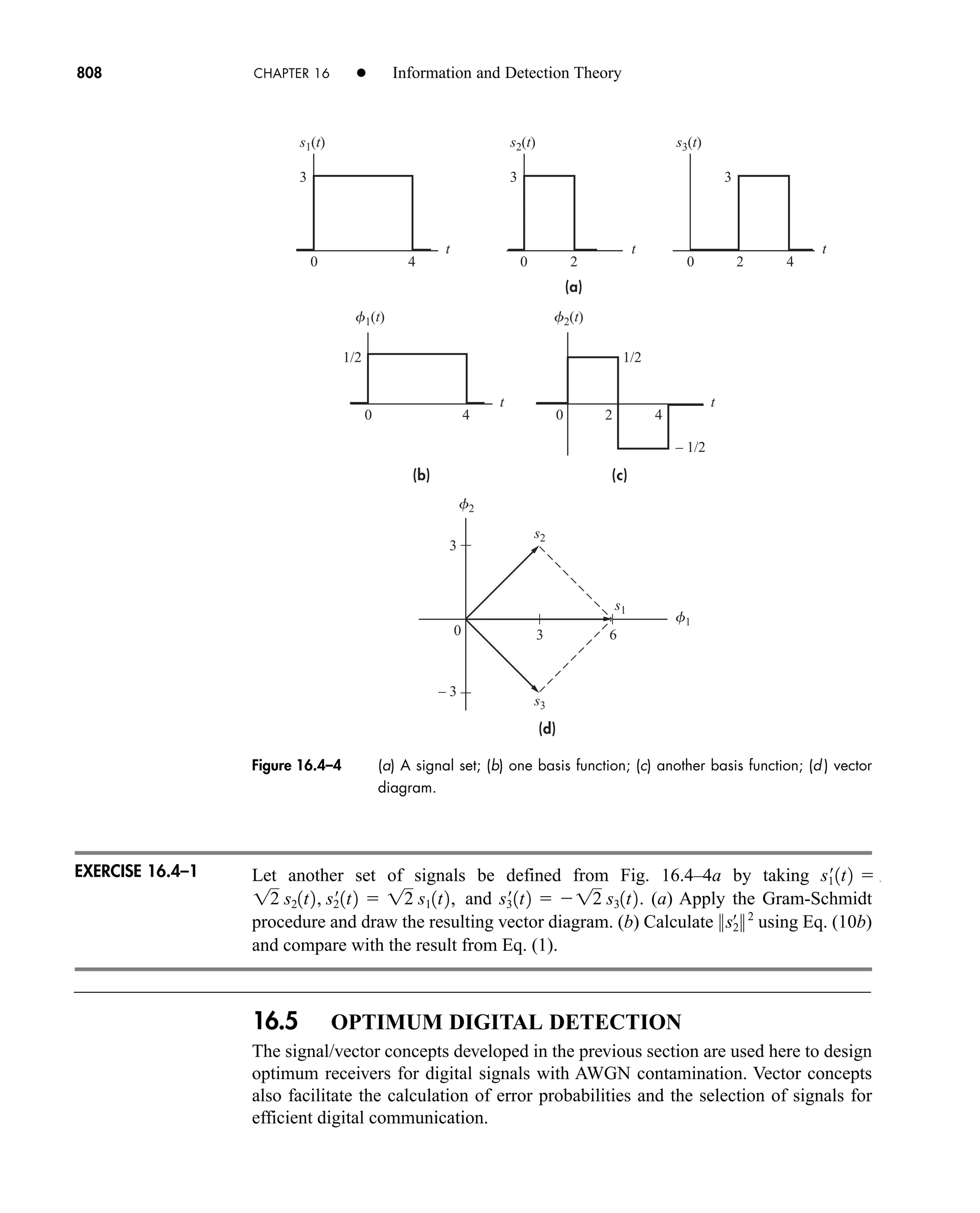
2.6 DISCRETE TIME SIGNALS AND THE DISCRETE
FOURIER TRANSFORM
It will be shown in Sect. 6.1 that if we sample a signal at a rate at least twice its
bandwidth, then it can be completely represented by its samples. Consider a rectan-
gular pulse train that has been sampled at rate fs 1/Ts and is shown in Fig. 2.6–1a.
It is readily observed that the sampling interval is t Ts. The samples can be
expressed as
(1a)
Furthermore, if our sampler is a periodic impulse function, we have
(1b)
Then we drop the Ts to get
(1c)
where x(k) is a discrete-time signal, an ordered sequence of numbers, possibly com-
plex, and consists of k 0, 1, . . . N 1, a total of N points.
It can be shown that because our sampler is a periodic impulse function
(t kTs), then we can replace the Fourier transform integral of Eq. (4) of Sect. 2.2
with a summation operator, giving us
(2)
Alternatively, we can get Eq. (2) by converting the integral of Eq. (4), Sect. 2.2, to a sum-
mation and changing dt → t Ts. Function X(n) is the Discrete Fourier transform
(DFT), written as DFT[x(k)] and consisting of N samples, where each sample is spaced
at a frequency of 1/(NTs) fs/N Hz. The DFT of the sampled signal of Fig. 2.6–1a is
shown in Fig. 2.6–1b. Note how the DFT spectrum repeats itself every N samples or
every fs Hz. The DFT is computed only for positive N. Note the interval from n → (n 1)
represents fs /N Hz, and thus the discrete frequency would then be
(3)
Observe that both x(k) and X(n) are an ordered sequence of numbers and thus can
easily be processed by a computer or some other digital signal processor (DSP).
n S fn nfsN
X1n2 a
N1
k0
x1k2ej2pnkN
n 0, 1 p N
x1k2 x1kTs 2
x1kTs 2 x1t2d1t kTs 2
x1t2|tkTs
x1kTs 2
EXERCISE 2.5–3
car80407_ch02_027-090.qxd 12/8/08 11:04 PM Page 80](https://image.slidesharecdn.com/communicationsystemsanintro-a-241115060943-61721fa8/75/Communication_Systems__An_Intro_-_A-_Bruce_Carlson_-pdf-102-2048.jpg)
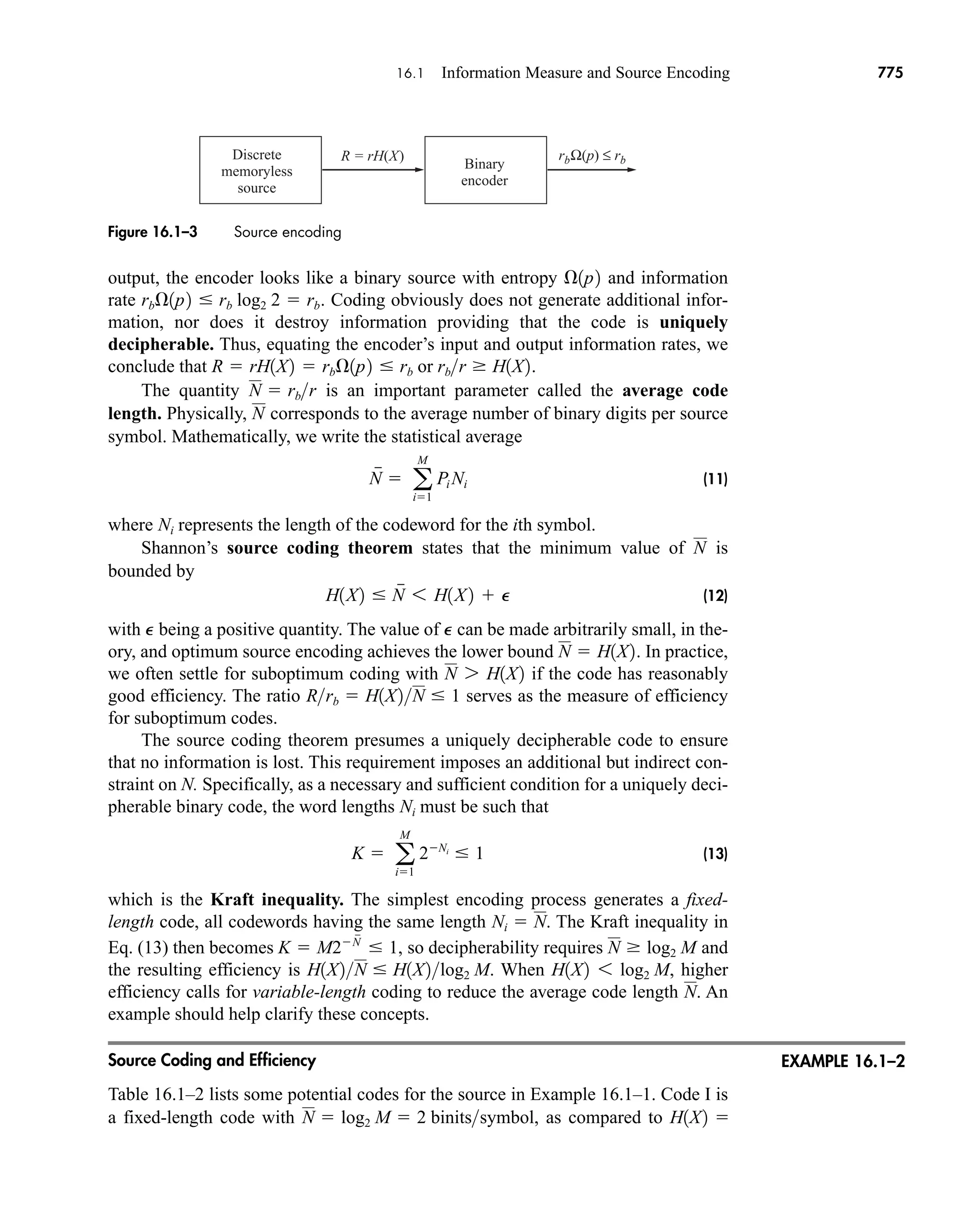
![2.6 Discrete Time Signals and the Discrete Fourier Transform 81
The corresponding inverse discrete Fourier transform (IDFT) is
(4)
Equations (2) and (4) can be separated into their real and imaginary components giving
and
Sect. 6.1 will discuss how x(t) is reconstructed from from X(n) or x(k).
In examining Eqs. (2) and (4) we see that the number of complex multiplica-
tions required to do a DFT or IDFT is N2
. If we are willing to work with N 2y
sam-
ples, where y is an integer, we can use the Cooley-Tukey technique, otherwise
known as the fast Fourier transform (FFT) and inverse FFT (IFFT), and thereby
reduce the number of complex multiplications to This technique greatly
N
2
log2 N.
xR1k2 Re3x1k2 4 and xI 1k2 Im3x1k2 4.
XR1n2 Re3X1n2 4 and XI 1n2 Im3X1n2 4
x1k2 IDFT3X1n2 4
1
N a
N
n0
X1n2ej2pnkN
k 0, 1 p N
Figure 2.6-1 (a) Sampled rectangular pulse train with (b) corresponding N 16 point
DFT[x(k)]. Also shown is the analog frequency axis.
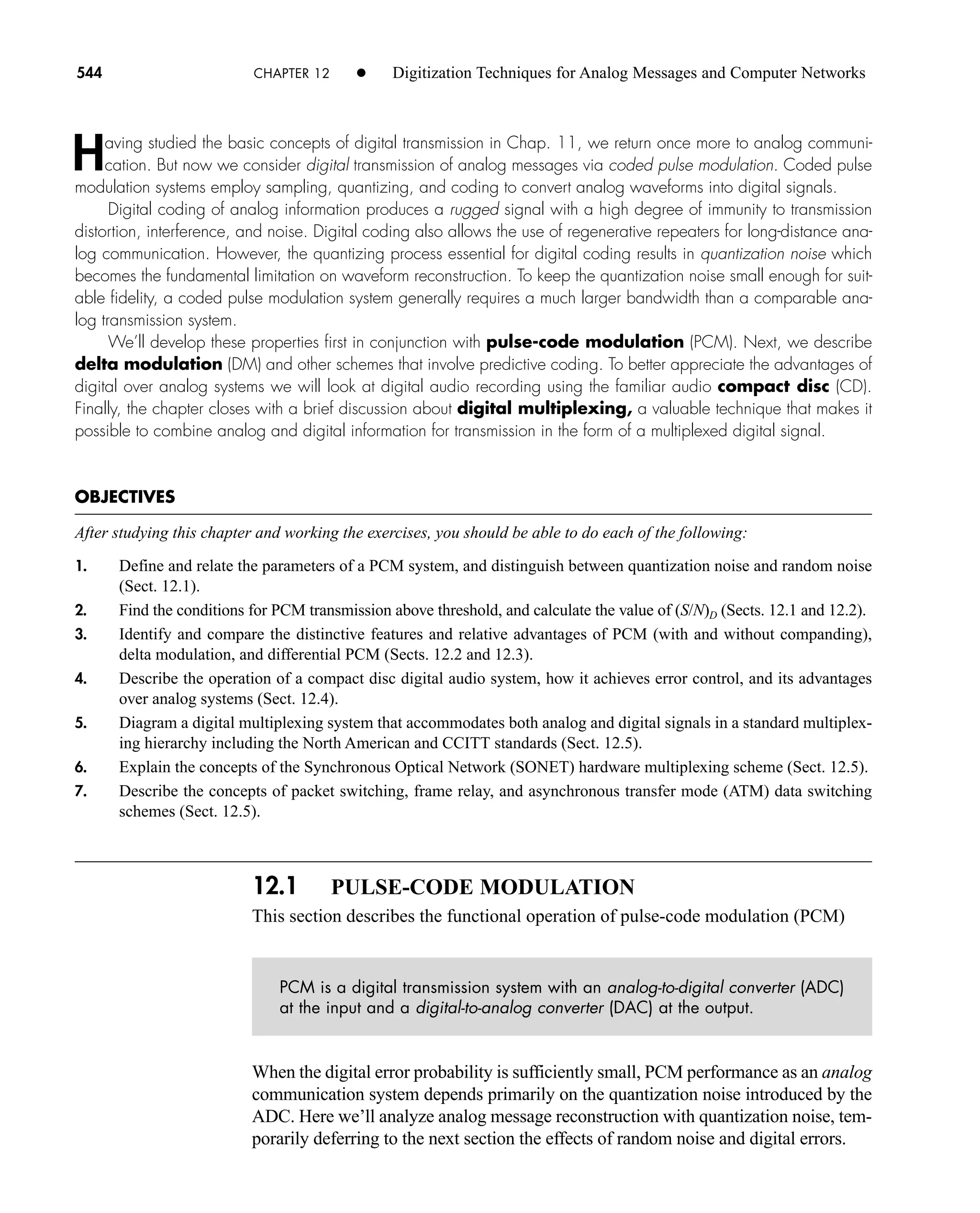
0 1
0 1 2 3 8 13 14 15 16
8 15 16
f
N
2
N
2
0 fs
2
fs
N
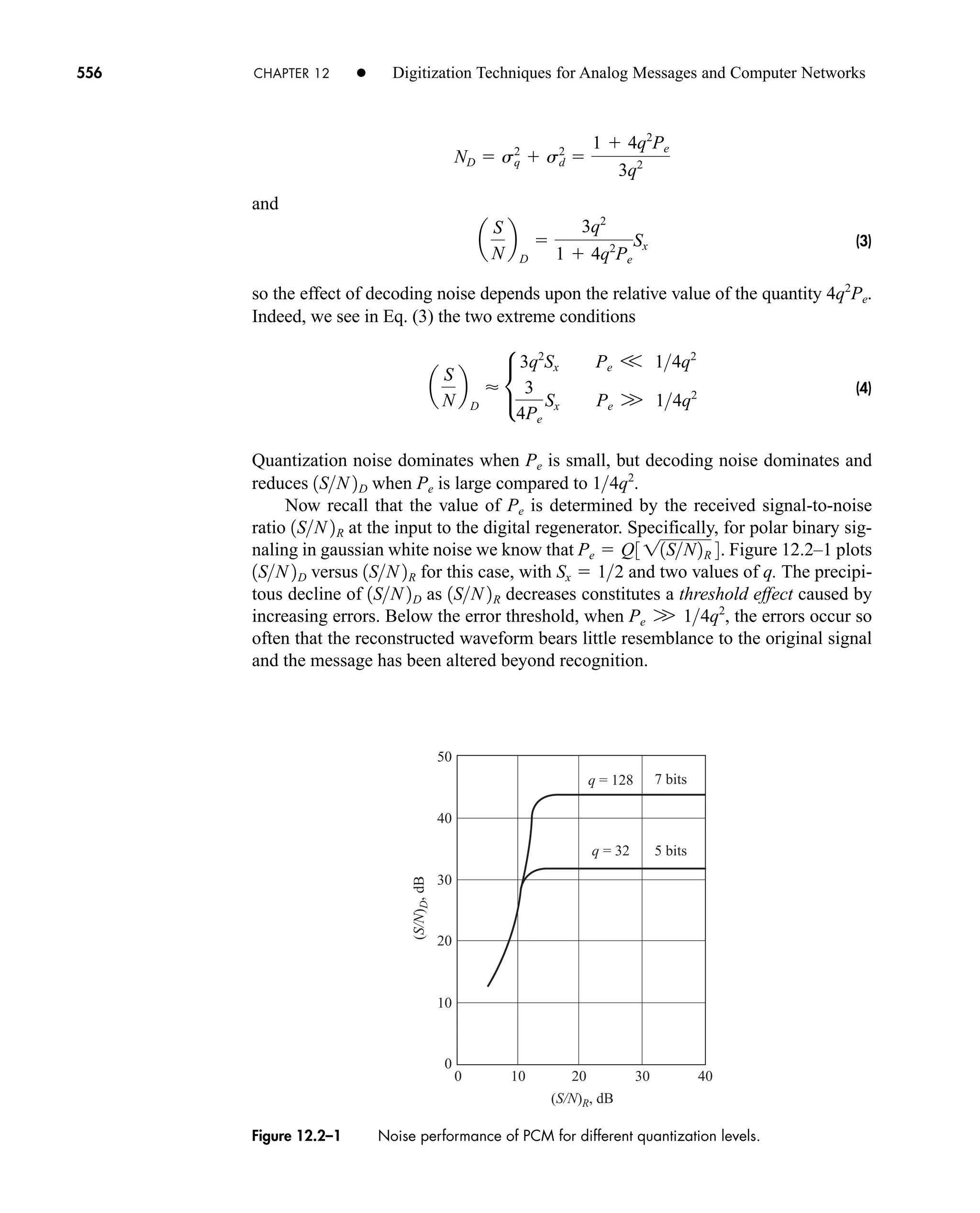
∆f =
∆t = Ts
n
X(n)
x(k)
(b)
N−1
N−1
k
A1
A2
(a)
fs
car80407_ch02_027-090.qxd 12/8/08 11:04 PM Page 81](https://image.slidesharecdn.com/communicationsystemsanintro-a-241115060943-61721fa8/75/Communication_Systems__An_Intro_-_A-_Bruce_Carlson_-pdf-103-2048.jpg)
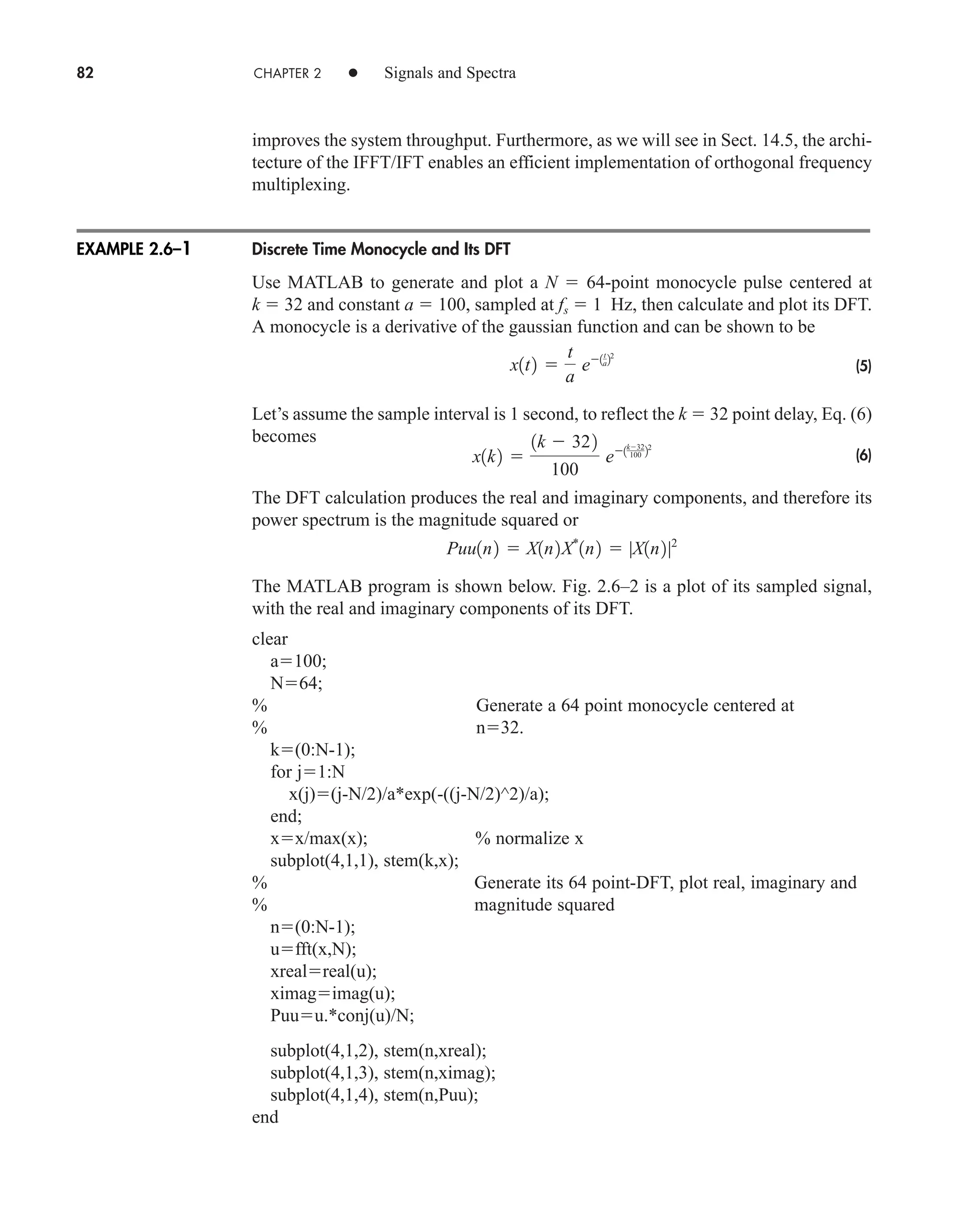
![2.6 Discrete Time Signals and the Discrete Fourier Transform 83
Note that k to (k 1) corresponds to a 1-second interval and n to (n 1) corre-
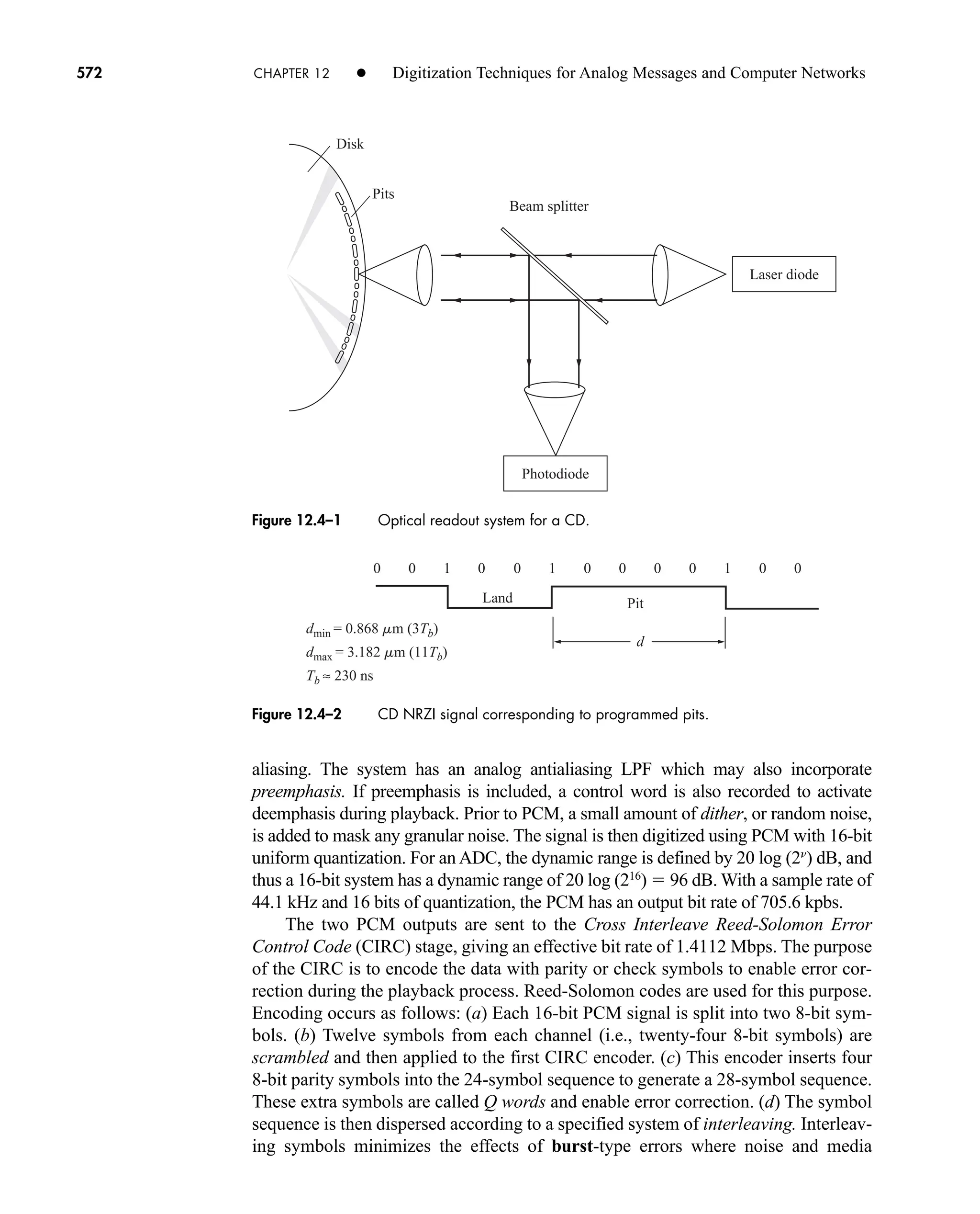
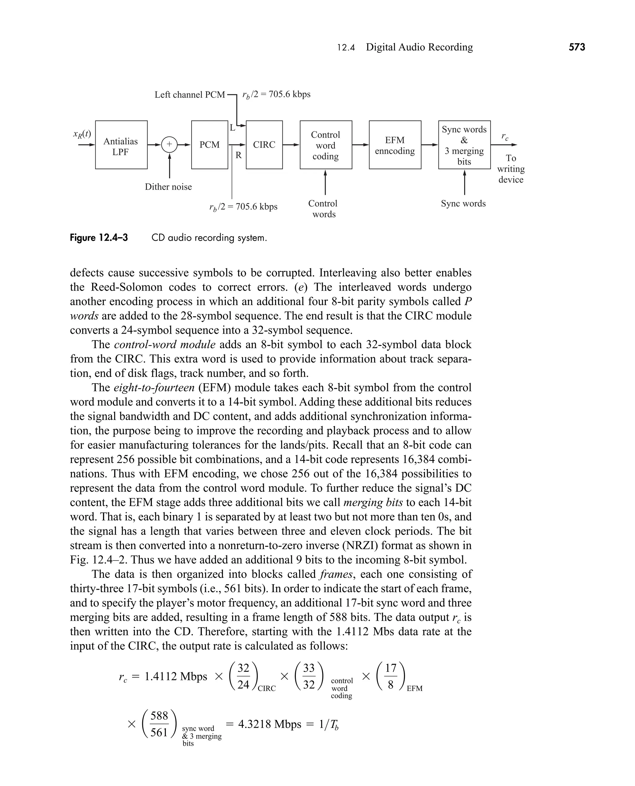
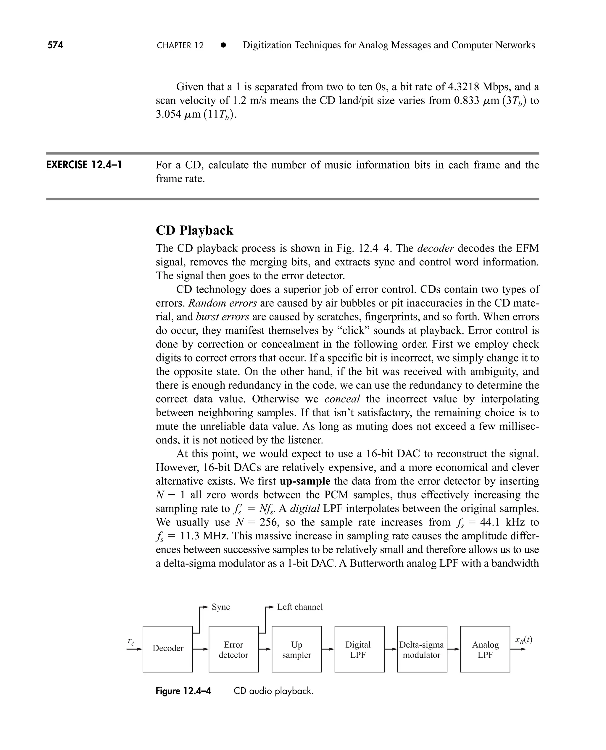
sponds to a 1/64 Hz interval. Therefore, the graphs of x(k) and X(n) span 64 sec-
onds and 64 Hz respectively.
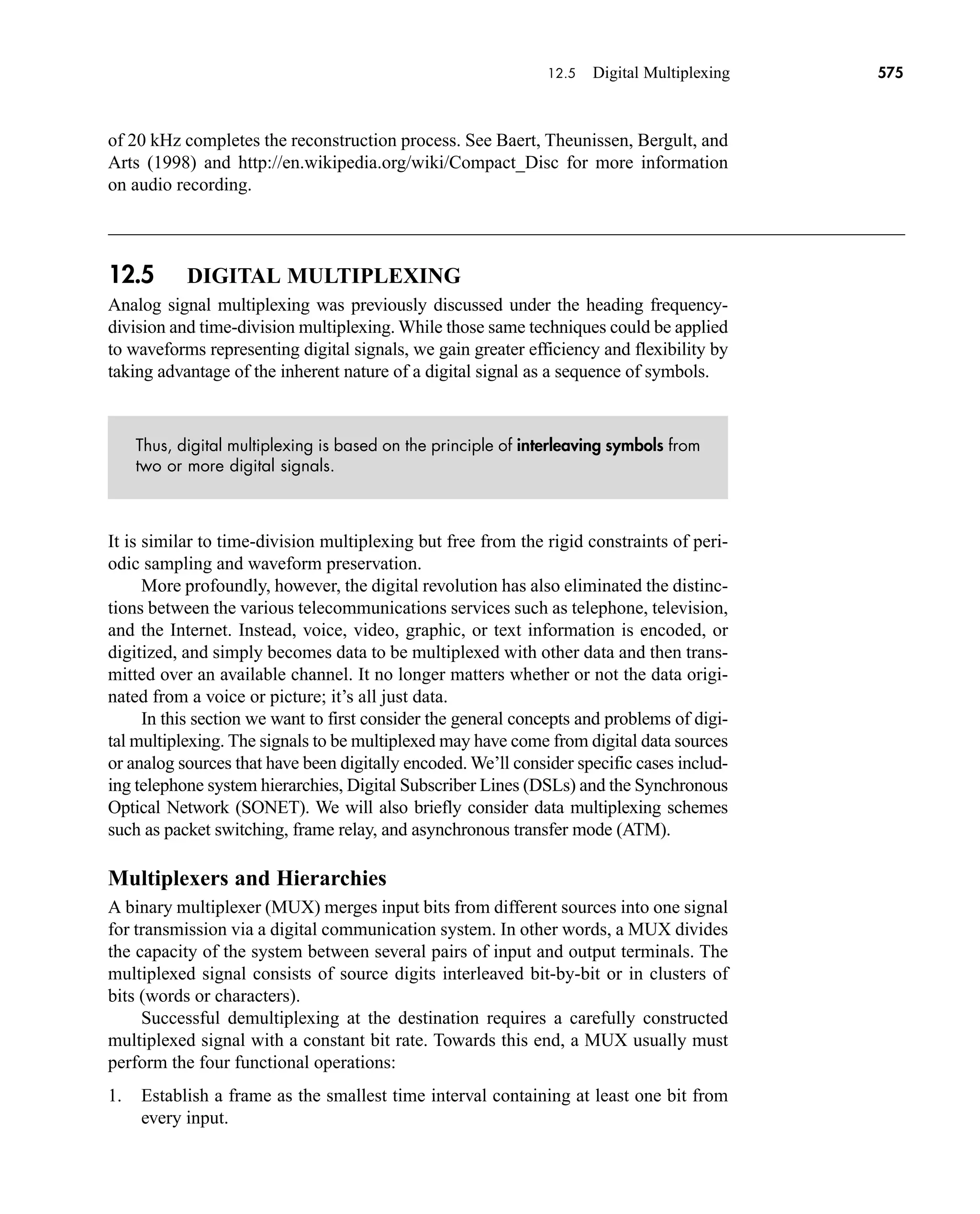
Derive Eq. (2). Assume the signal was sampled by an impulse train.
Convolution Using the DFT
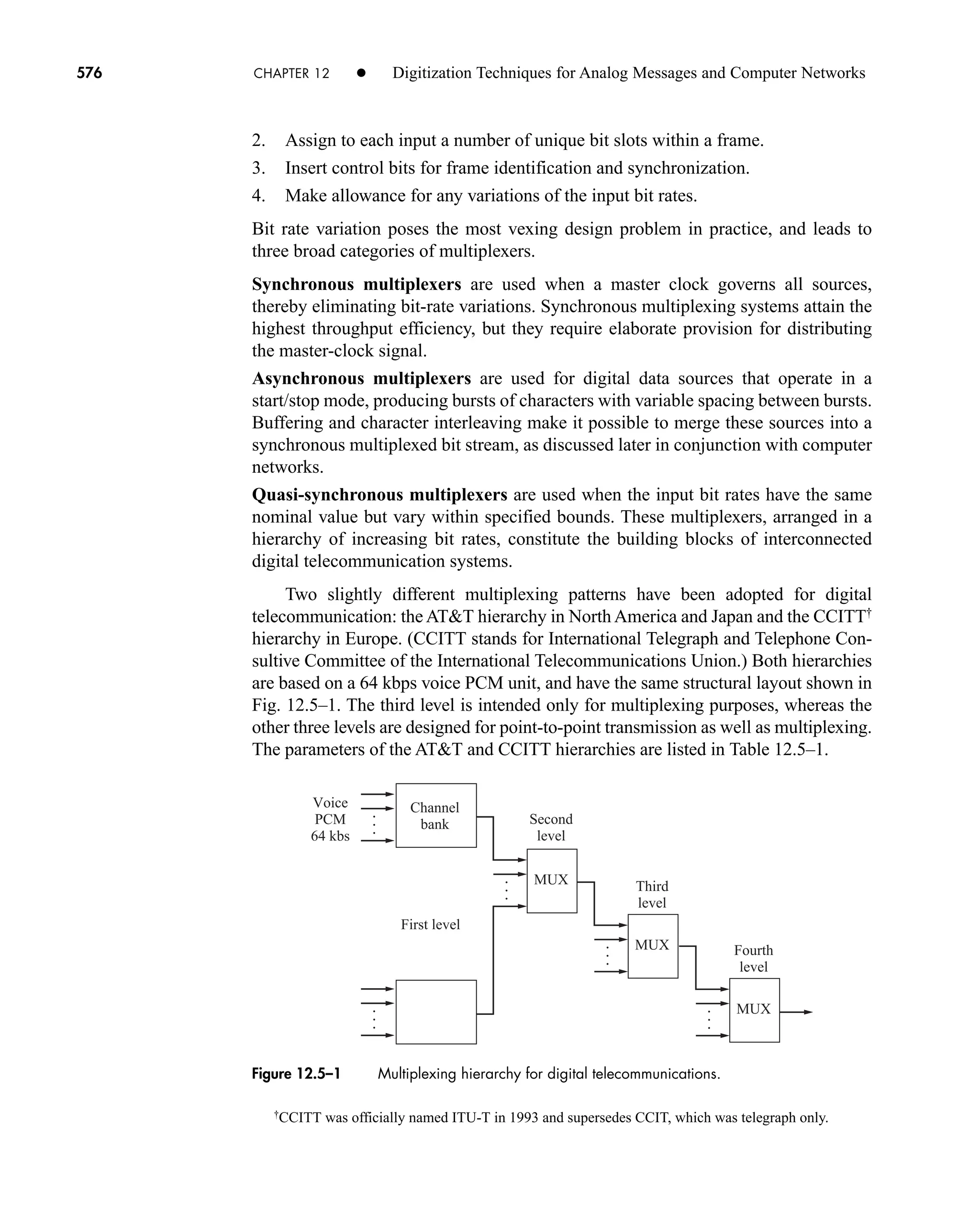
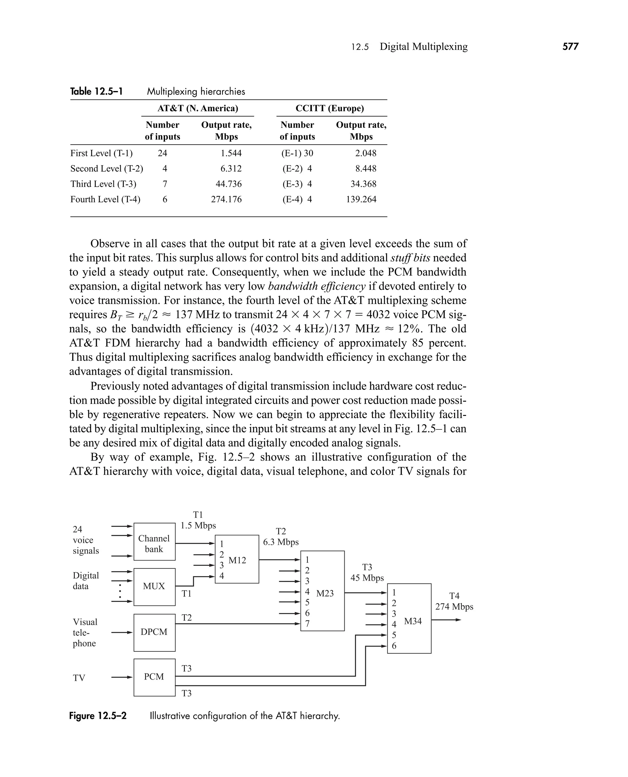
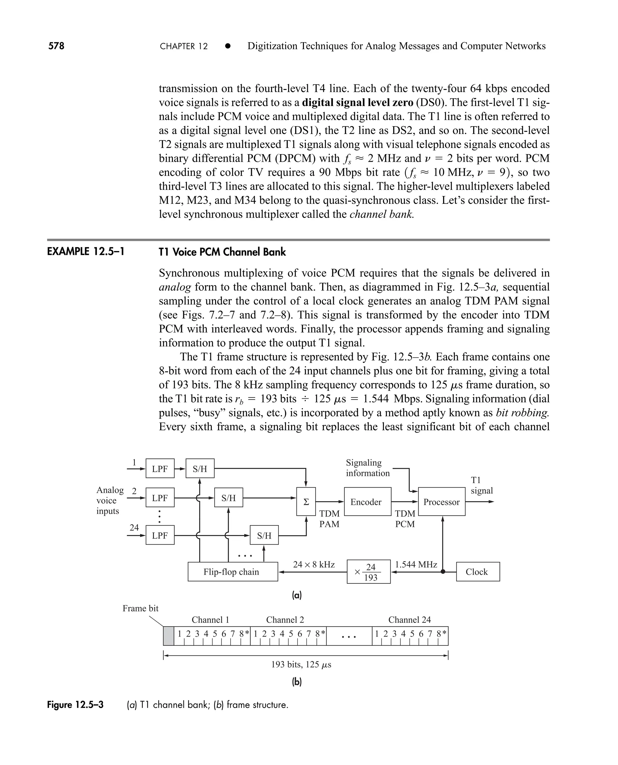
Just as with the continuous-time system, the output of a discrete-time system is the
linear convolution of the input with the system’s impulse response system, or simply
(7)
where the lengths of x(k) and h(k) are bounded by N1 and N2 respectively, the length of
y(k) is bounded by N (N1 N2 1), y(k) and x(k) are the sampled versions of y(t)
and x(t) respectively, and * denotes the linear convolution operator. The system’s
discrete-time impulse response function, h(k), is approximately equal to its analog
counterpart, h(t).†
However, for reasons of brevity, we will not discuss under what con-
ditions they are closely equal. Note that we still have the DFT pair of
where H(k) is discrete system response.
h1k2 4 H1k2
y1k2 x1k2 * h1k2 a
N
l0
x1l2h1k l2
Figure 2.6-2 Monocycle and its DFT: (a) Monocycle x(k) with Ts 1 s.; (b) Re[X(n)];
(c) Im[X(n)]; (d) Puu(n) |X(n)|2
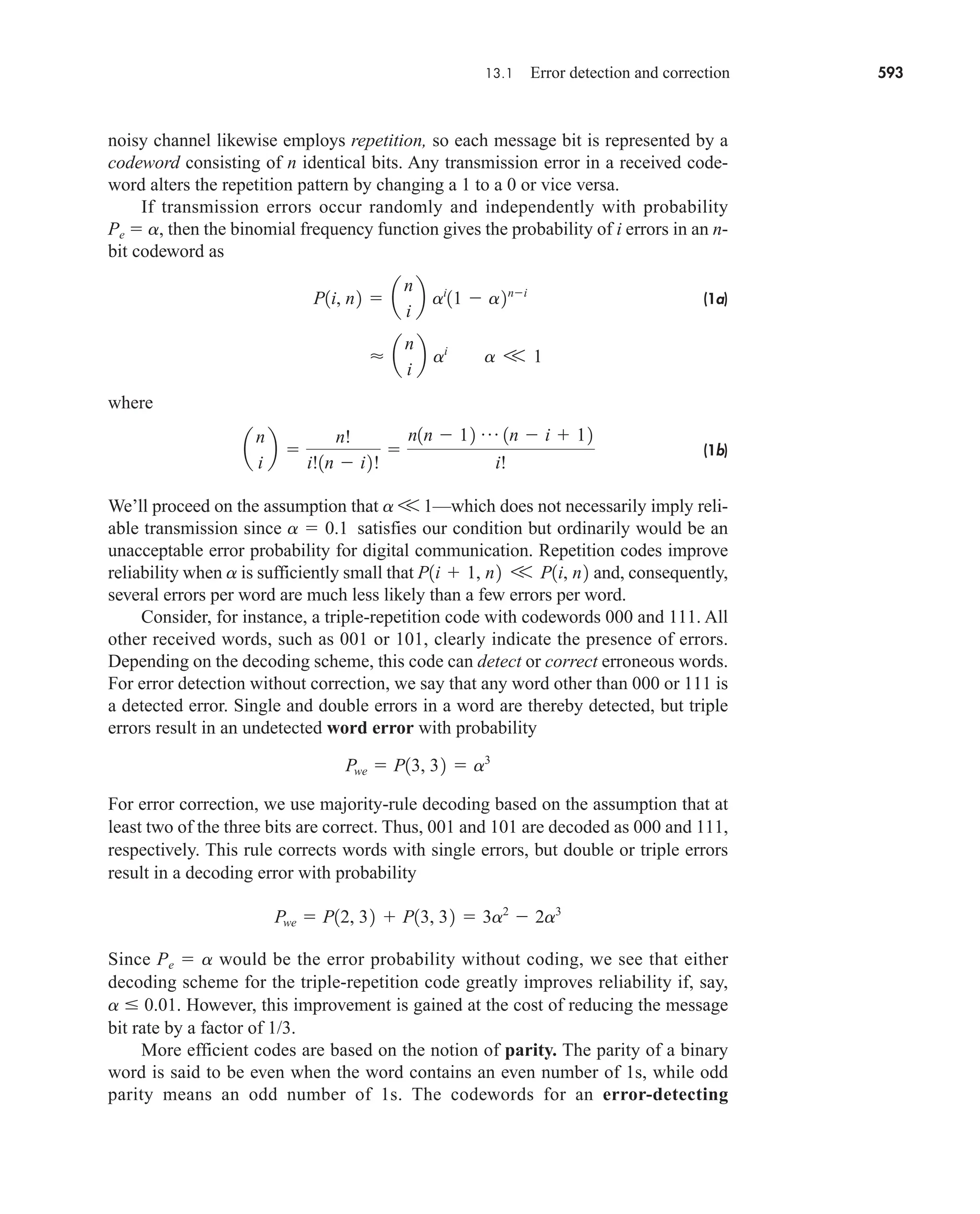
.
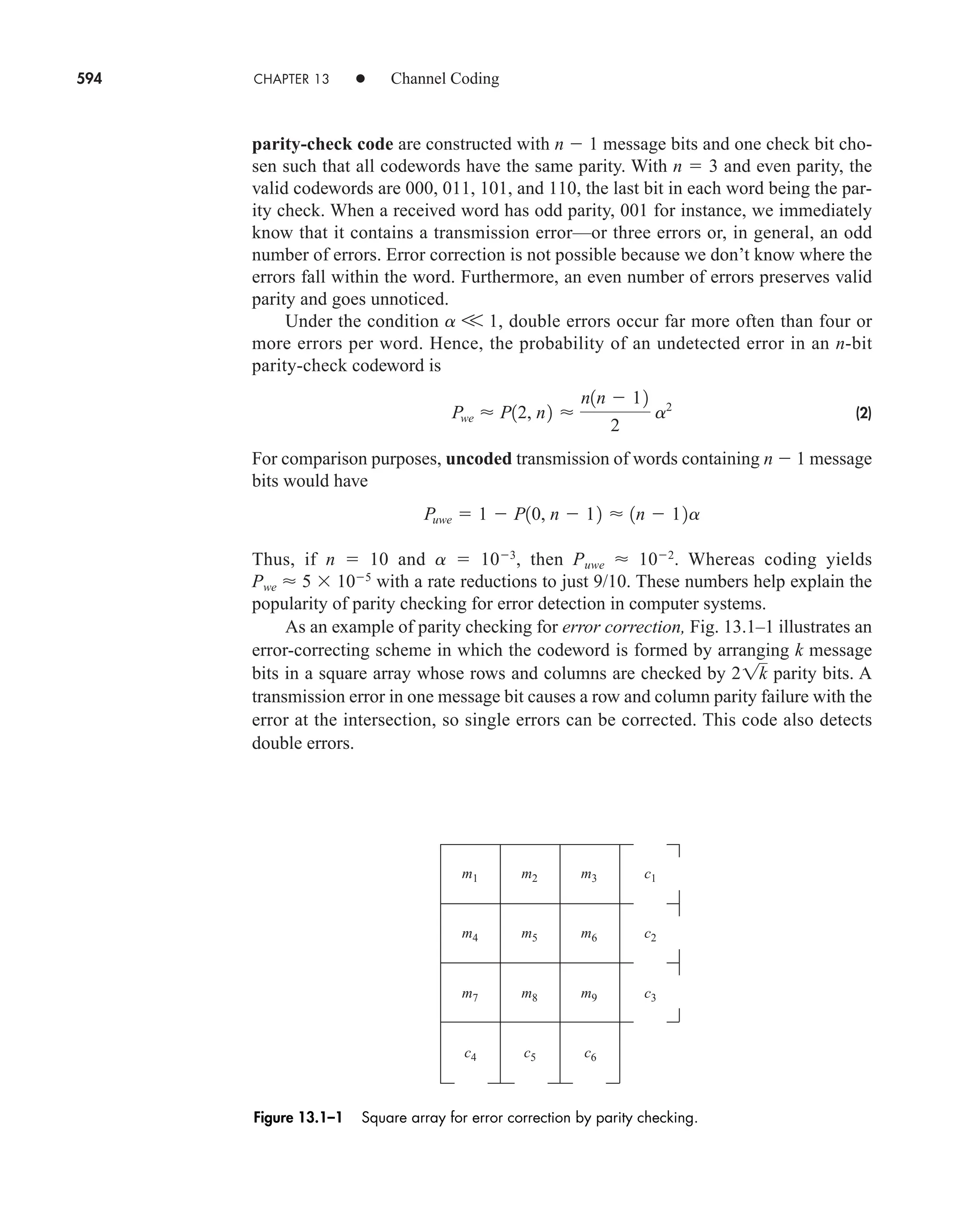
x(k)
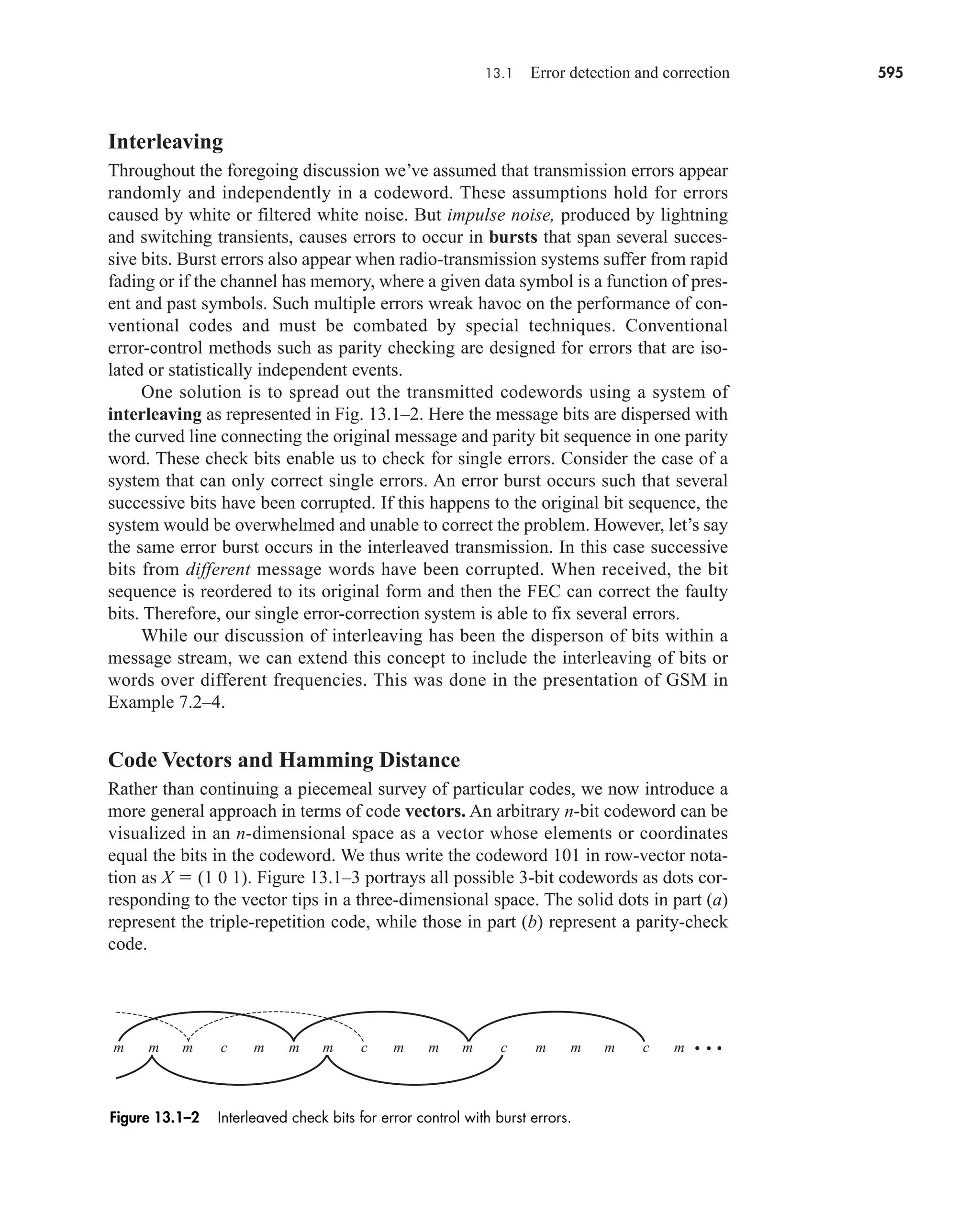
XR(n)
XI(n)
Puu(n)
n
n
n
n
k
(a)
(b)
(c)
(d)
1
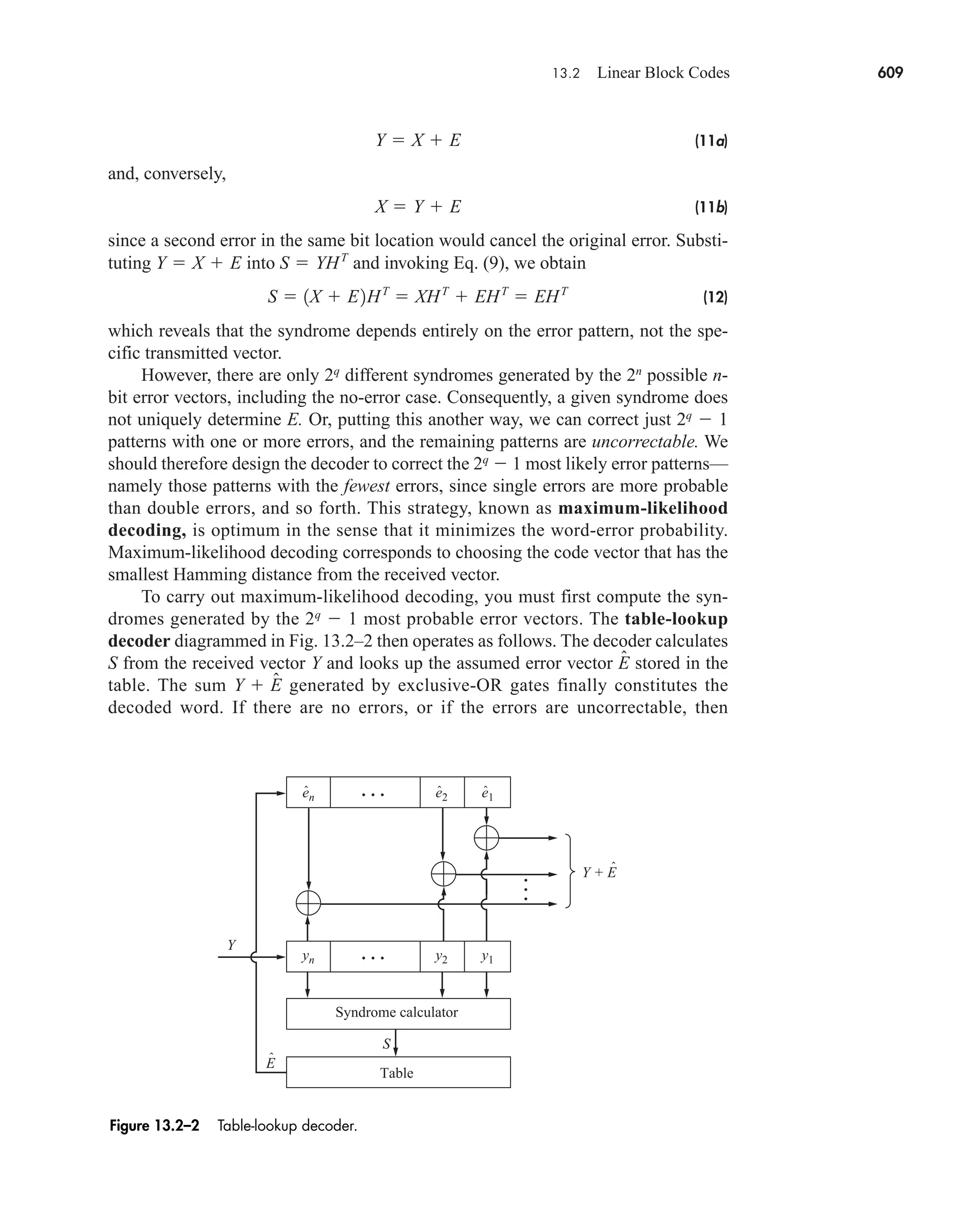
0
0 10 20 30 40 50 60 70
−1
5
0
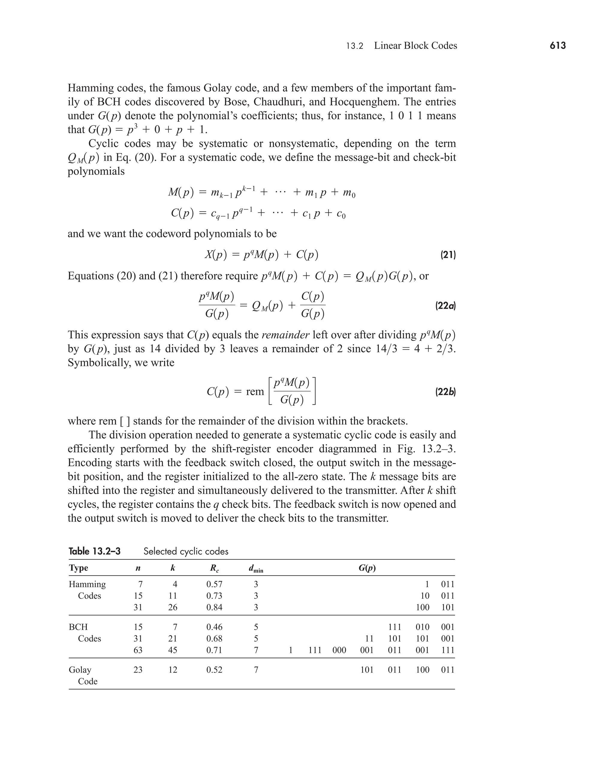
0 10 20 30 40 50 60 70
−5
20
0
0 10 20 30 40 50 60 70
−20
4
2
0 10 20 30 40 50 60 70
0
EXERCISE 2.6–1
†
Function h(k) ≅ h(t) if fs Nyquist rate. See Ludeman (1986) for more information.
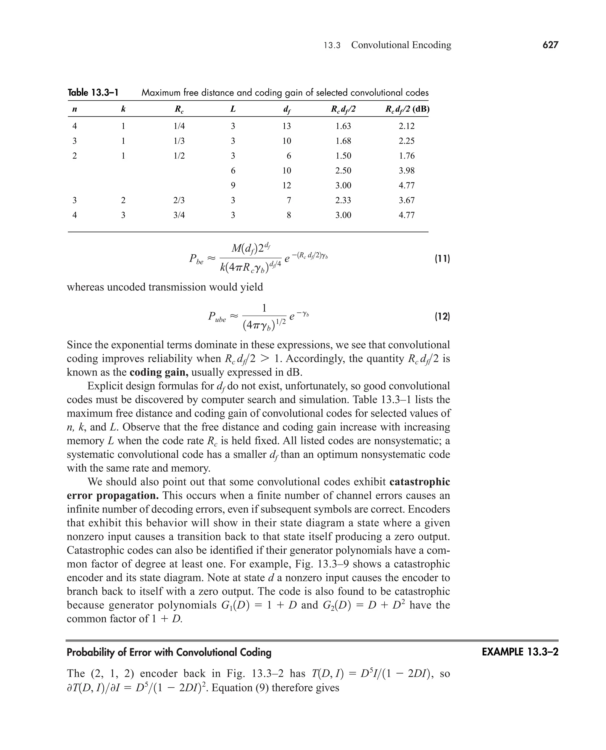
W
car80407_ch02_027-090.qxd 12/8/08 11:04 PM Page 83](https://image.slidesharecdn.com/communicationsystemsanintro-a-241115060943-61721fa8/75/Communication_Systems__An_Intro_-_A-_Bruce_Carlson_-pdf-105-2048.jpg)
![84 CHAPTER 2 • Signals and Spectra
If
then we have
(8)
where ⊗ denotes circular convolution. Circular convolution is similar to linear con-
volution, except both functions must be the same length, and the resultant function’s
length can be less than the bound of N1 N2 1. Furthermore, while the operation
of linear convolution adds to the resultant sequence’s length, with circular convolu-
tion, the new terms will circulate back to the beginning of the sequence.
It is advantageous to use specialized DFT hardware to perform the computa-
tions, particularly as we will see in Sect. 14.5. If we are willing to constrain the
lengths of N1 N2 and N (2N1 1), then the linear convolution is equal to the cir-
cular convolution,
(9a)
[9b]
(9c)
and
(9d)
The lengths of x1(k) and x2(k) can be made equal by appending zeros to the sequence
with the shorter length. Thus, just as the CFT replaces convolution in continuous-
time systems, so can the DFT be used to replace linear convolution for discrete-time
systems. For more information on the the DFT and circular convolution, see Oppen-
heim, Schafer, and Buck (1999).
2.7 QUESTIONS AND PROBLEMS
Questions
1. Why would periodic signals be easier to intercept than nonperiodic ones?
2. Both the H(f) sinc(ft) and H(f) sinc2
(ft) have low-pass-frequency responses,
and thus could be used to reconstruct a sampled signal. What is their equivalent
operation in the time domain?
3. You have designed a noncommunications product that emits radio frequency
(RF) interference that exceeds the maximum limits set by the FCC. What signal
shapes would most likely be the culprit?
y1k2 IDFT3Y1n2 4
Y1k2 DFT3x11n2 z x21n2 4
Y1n2 DFT3x11k2 4 DFT3x21k2 4
y1k2 x11k2 * x21k2 x11k2 z x21k2
x11k2 z x21k2 4 X11n2X21n2
X11n2 DFT3x1 1k2 4 and X2 1n2 DFT3x21k2 4
car80407_ch02_027-090.qxd 12/8/08 11:04 PM Page 84](https://image.slidesharecdn.com/communicationsystemsanintro-a-241115060943-61721fa8/75/Communication_Systems__An_Intro_-_A-_Bruce_Carlson_-pdf-106-2048.jpg)
![86 CHAPTER 2 • Signals and Spectra
2.1–6 Do Prob. 2.1–5 with y(t) A sin(2pt/T0) for t T0/2.
2.1–7‡
Consider a periodic signal with the half-wave symmetry property
y(tT0/2) y(t) , so the second half of any period looks like the first
half inverted. Show that cn 0 for all even harmonics.
2.1–8 How many harmonic terms are required in the Fourier series of a peri-
odic square wave with 50 percent duty cycle and amplitude A to rep-
resent 99 percent of its power?
2.1–9* Use Parseval’s power theorem to calculate the average power in the rec-
tangular pulse train with t/T0 1/4 if all frequencies above f 1/t are
removed. Repeat for the cases where all frequencies above f 2/t and
f 1/2t are removed.
2.1–10 Let y(t) be the triangular wave with even symmetry listed in Table T.2,
and let y(t) be the approximating obtained with the first three nonzero
terms of the trigonometric Fourier series. (a) What percentage of the
total signal power is contained in y(t)? (b) Sketch y(t) for t T0/2.
2.1–11 Do Prob. 2.1–10 for the square wave in Table T.2.
2.1–12‡
Calculate P for the sawtooth wave listed in Table T.2. Then apply Parse-
val’s power theorem to show that the infinite sum 1/12
1/22
1/32
. . . equals p2
/6.
2.1–13‡
Calculate P for the triangular wave listed in Table T.2. Then apply Parse-
val’s power theorem to show that the infinite sum 1/14
1/34
1/54
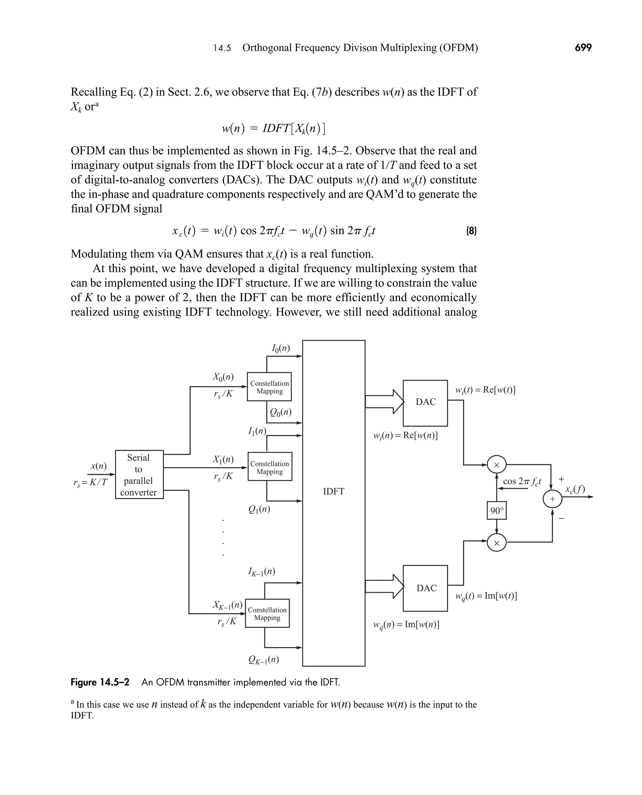
. . . equals p4
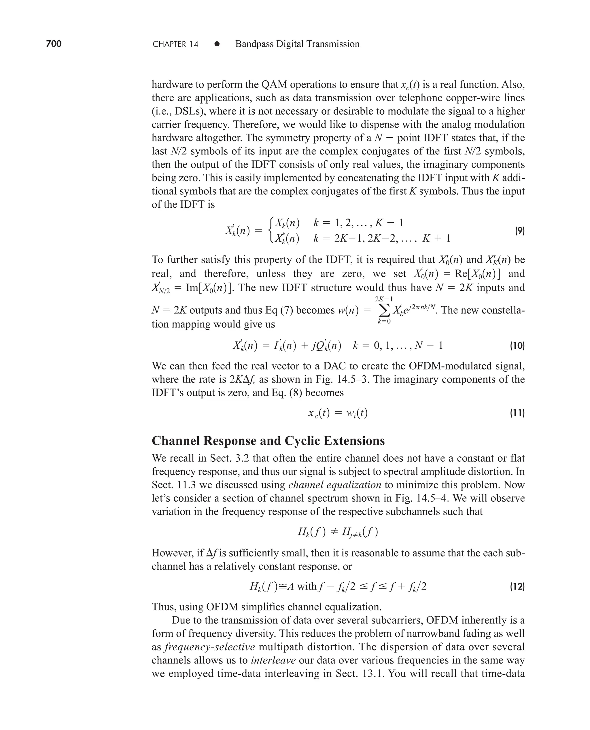
/96.
2.2–1 Consider the cosine pulse y(t) Acos(pt/t)Π(t/t). Show that
V(f) (At/2)[sinc(ft 1/2) sinc(ft 1/2)]. Then sketch and label
V(f) for f 0 to verify reciprocal spreading.
2.2–2 Consider the sine pulse y(t) Asin(2pt/t)Π(t/t). Show that V(f)
j(At/2)[sinc(ft 1) sinc(ft 1)]. Then sketch and label V(f) for
f 0 to verify reciprocal spreading.
2.2–3 Find V(f) when y(t) (A At/t)Π(t/2t). Express your result in terms
of the sinc function.
2.2–4* Find V(f) when y(t) (At/t)Π(t/2t). Express your result in terms of the
sinc function.
2.2–5 Given y(t) Π(t/t) with t 1 ms. Determine f0 such that
for all f f0
2.2–6 Repeat Prob. 2.2–5 for y(t) Λ (t/t).
V1f2 6
1
30
V102
*
Indicates answer given in the back of the book.
car80407_ch02_027-090.qxd 12/8/08 11:04 PM Page 86](https://image.slidesharecdn.com/communicationsystemsanintro-a-241115060943-61721fa8/75/Communication_Systems__An_Intro_-_A-_Bruce_Carlson_-pdf-108-2048.jpg)
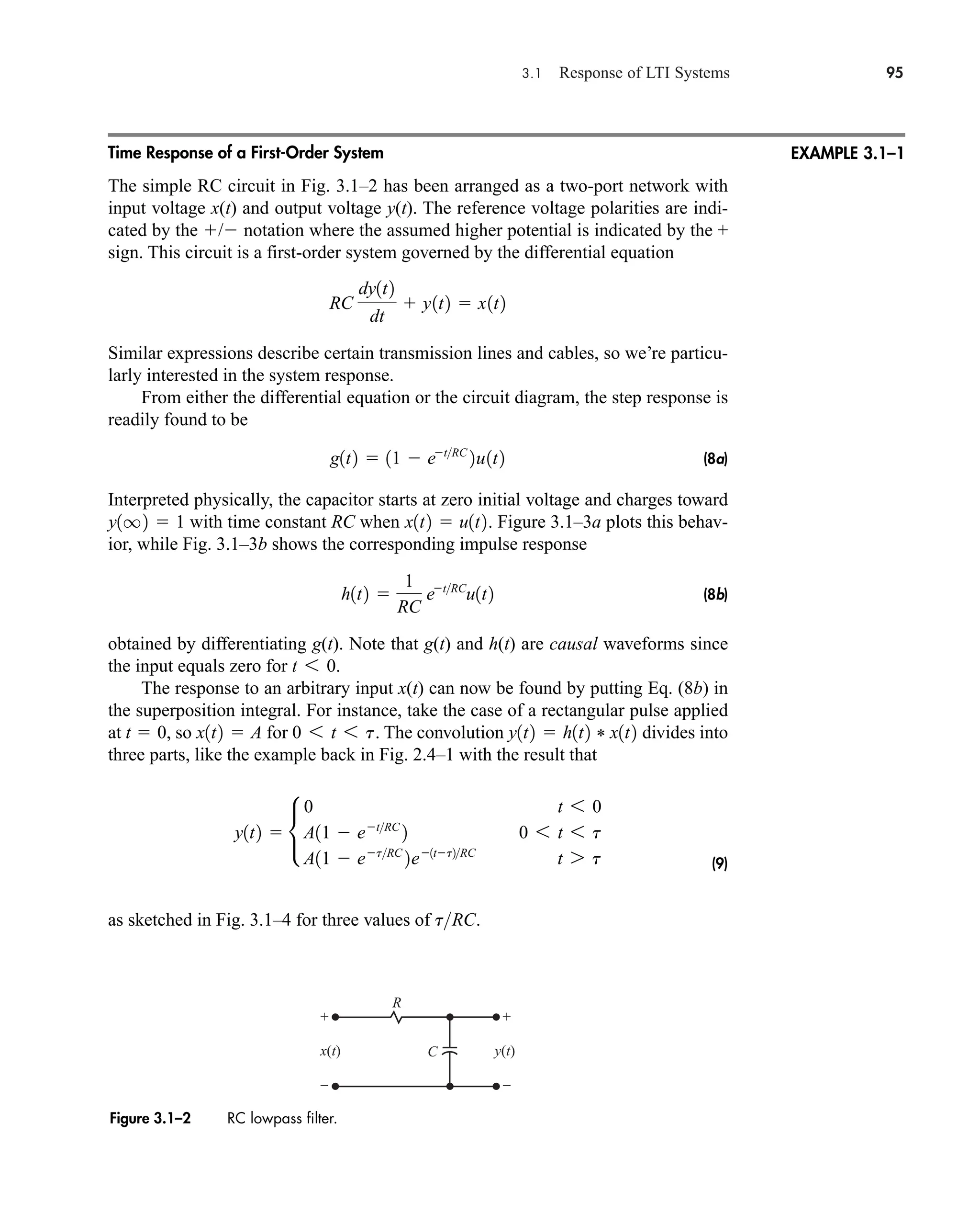
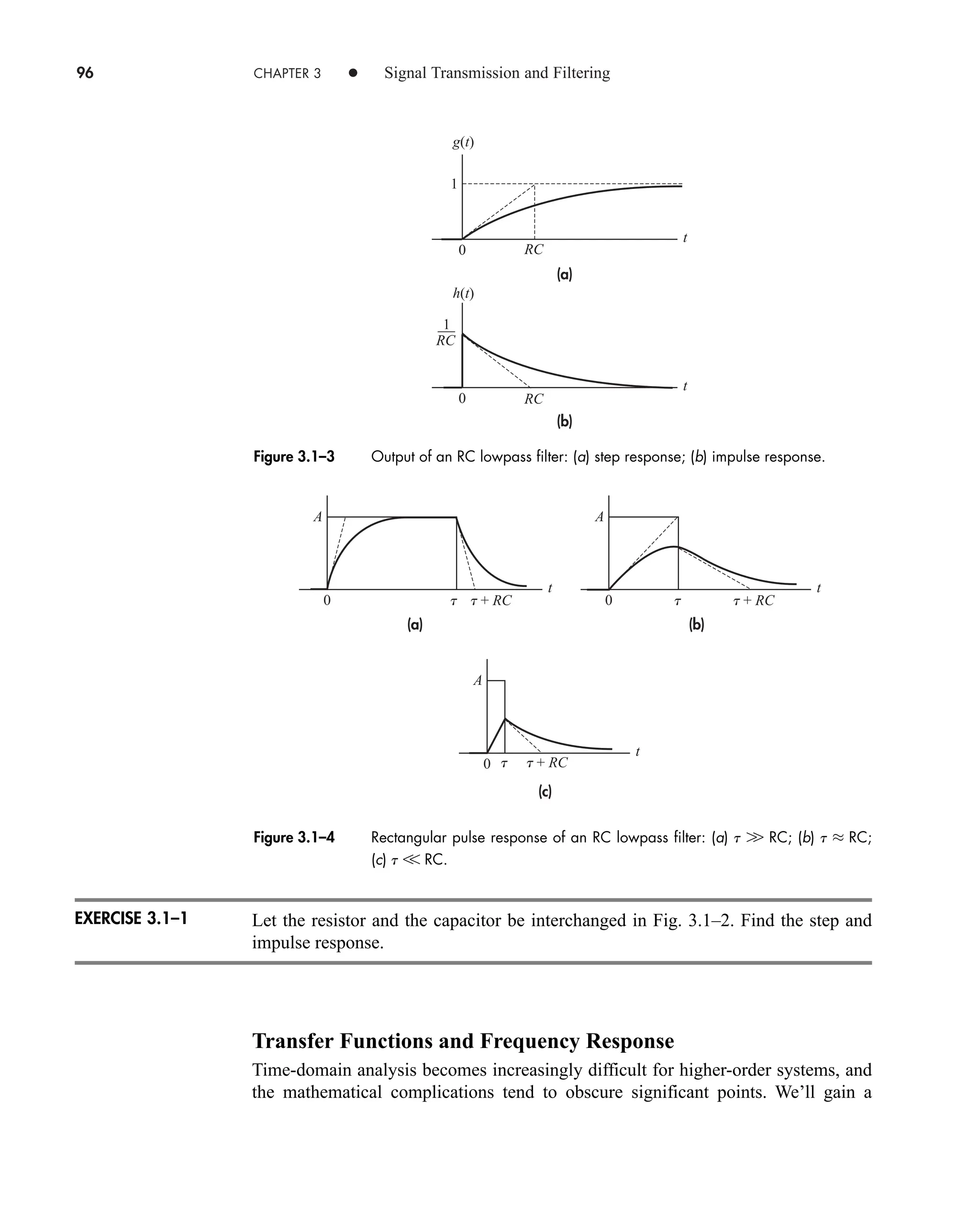
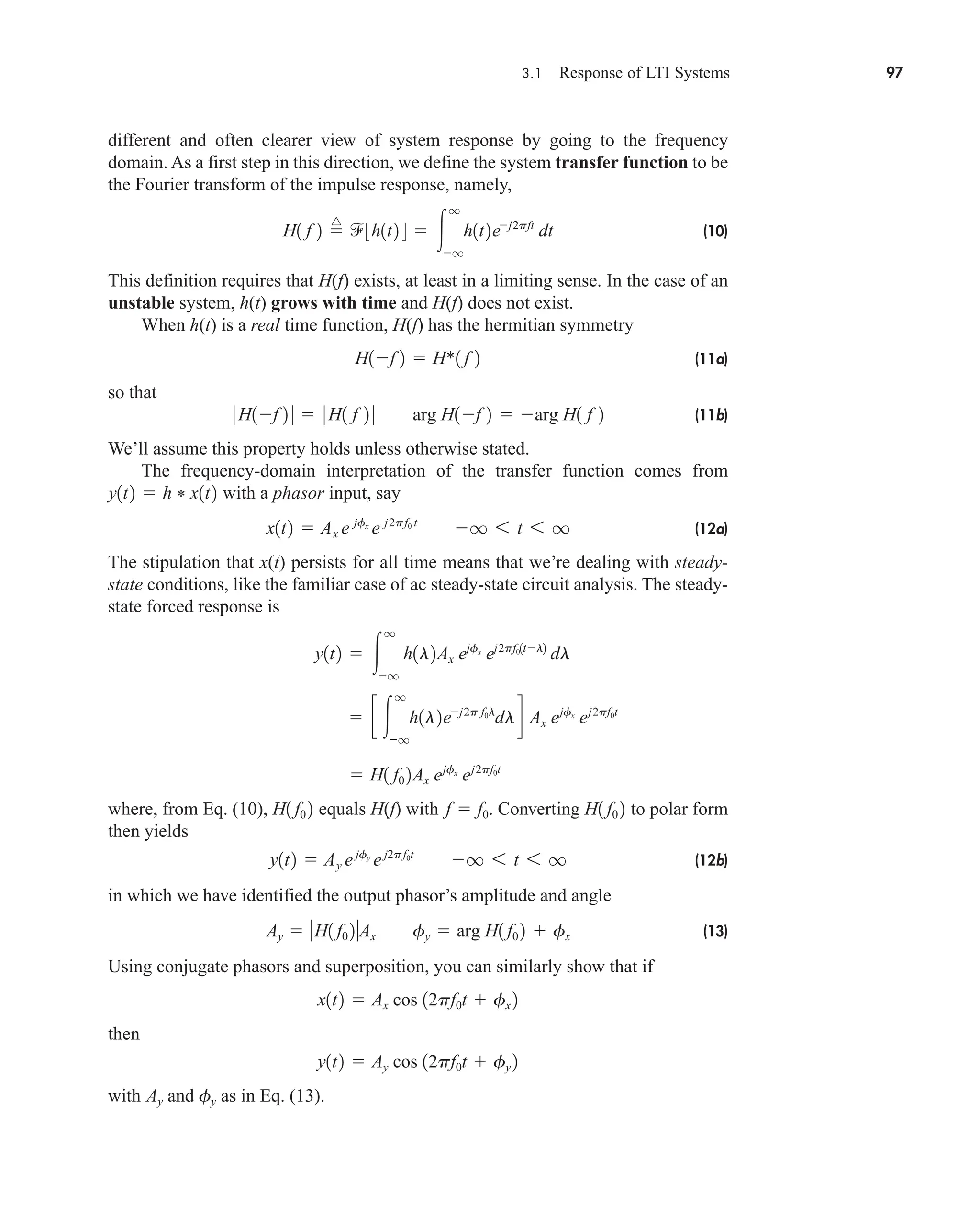
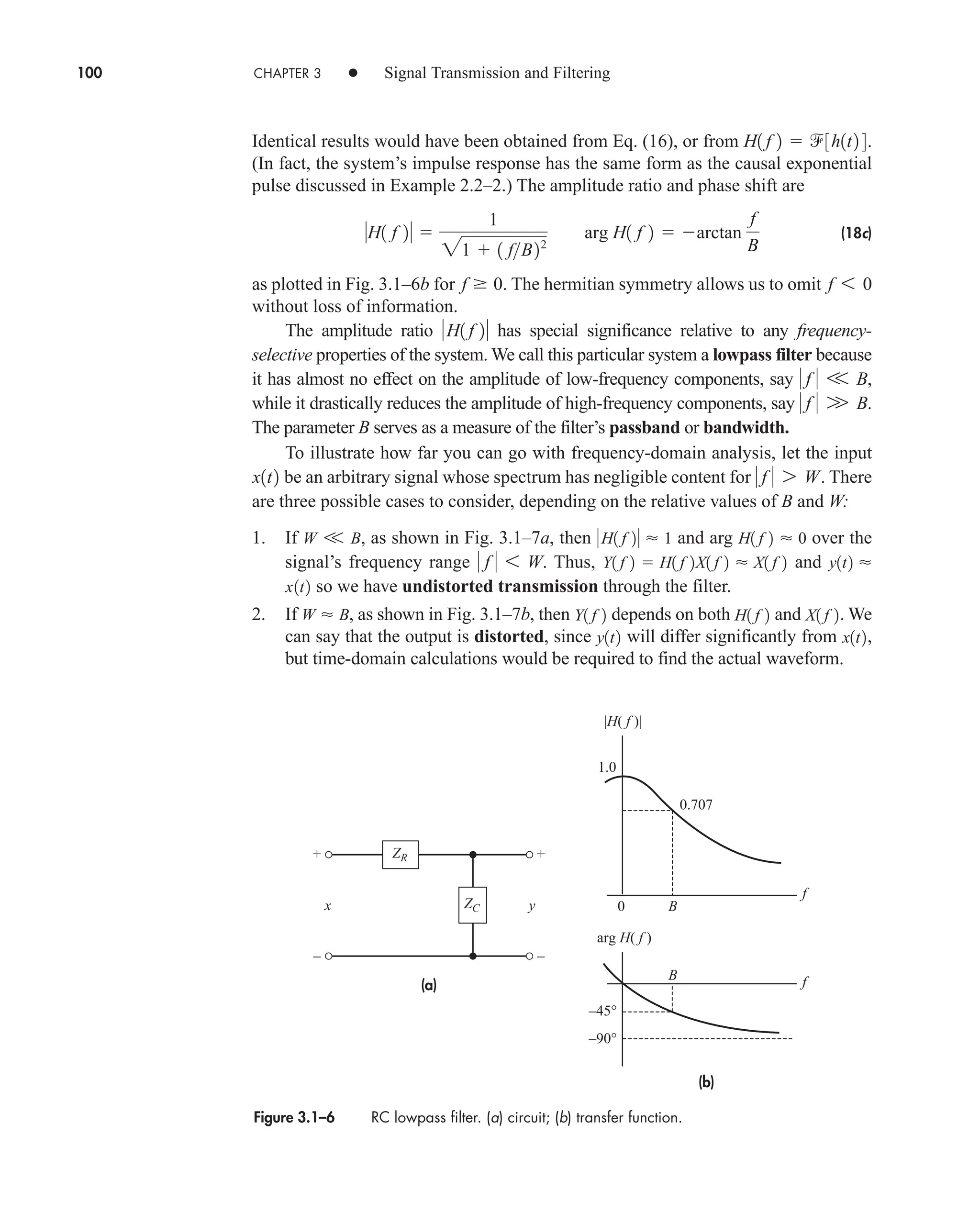
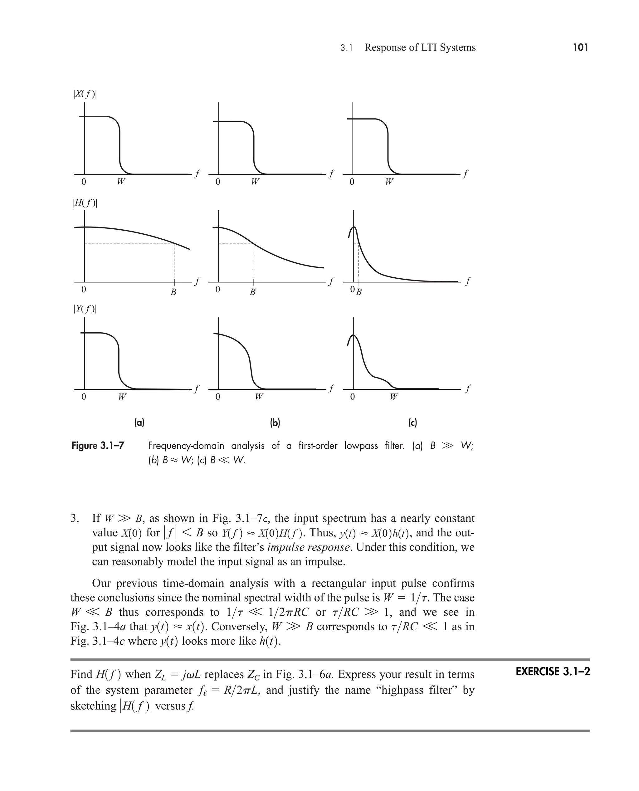
![3.1 Response of LTI Systems 93
x(t) y(t)
Black box
Input Output
System
Figure 3.1–1 System showing external input and output.
Here we’re concerned with the special but important class of linear time-
invariant systems—or LTI systems for short. We’ll develop the input–output rela-
tionship in the time domain using the superposition integral and the system’s impulse
response. Then we’ll turn to frequency-domain analysis expressed in terms of the sys-
tem’s transfer function.
Impulse Response and the Superposition Integral
Let Fig. 3.1–1 be an LTI system having no internal stored energy at the time the input
x(t) is applied. The output y(t) is then the forced response due entirely to x(t), as rep-
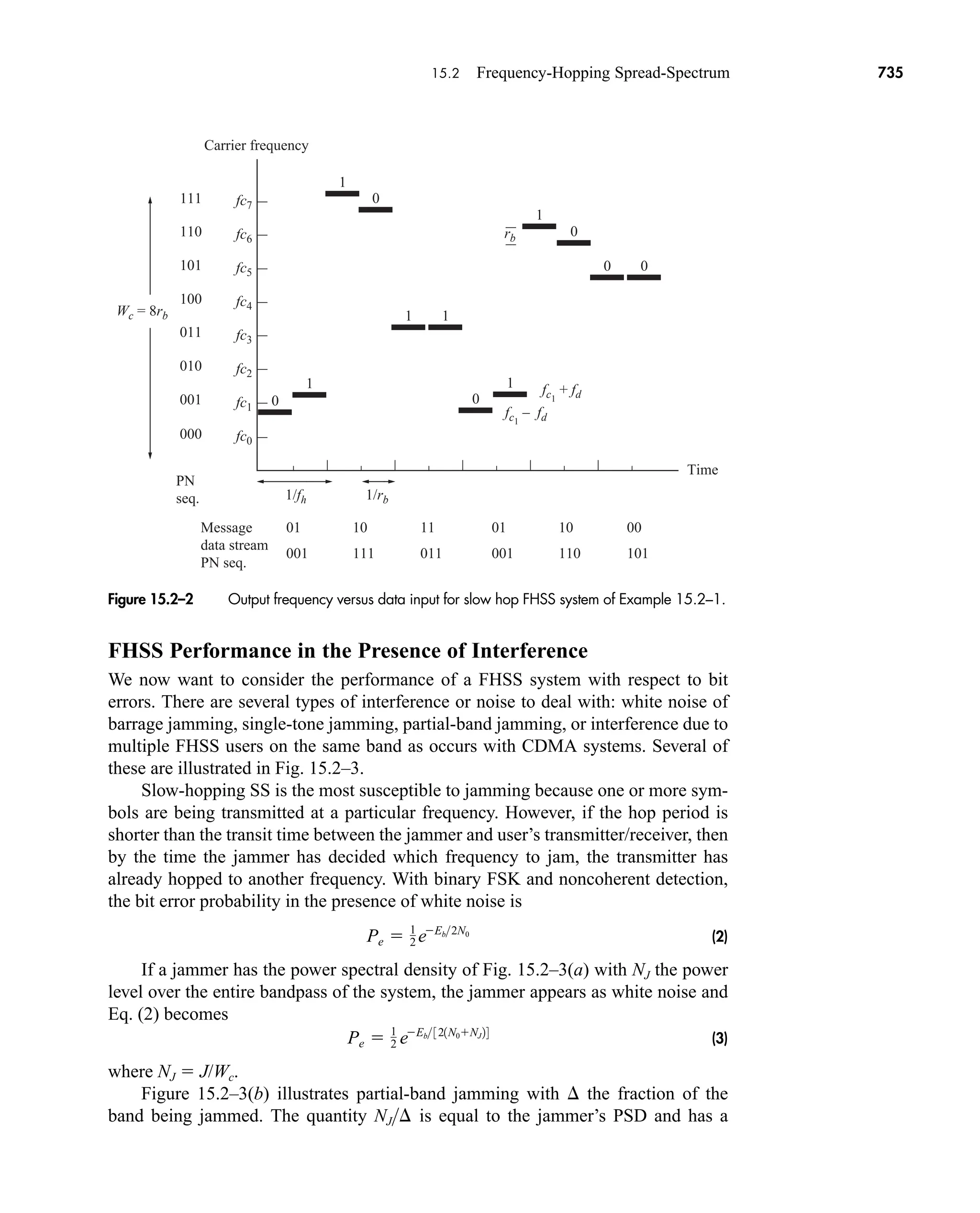
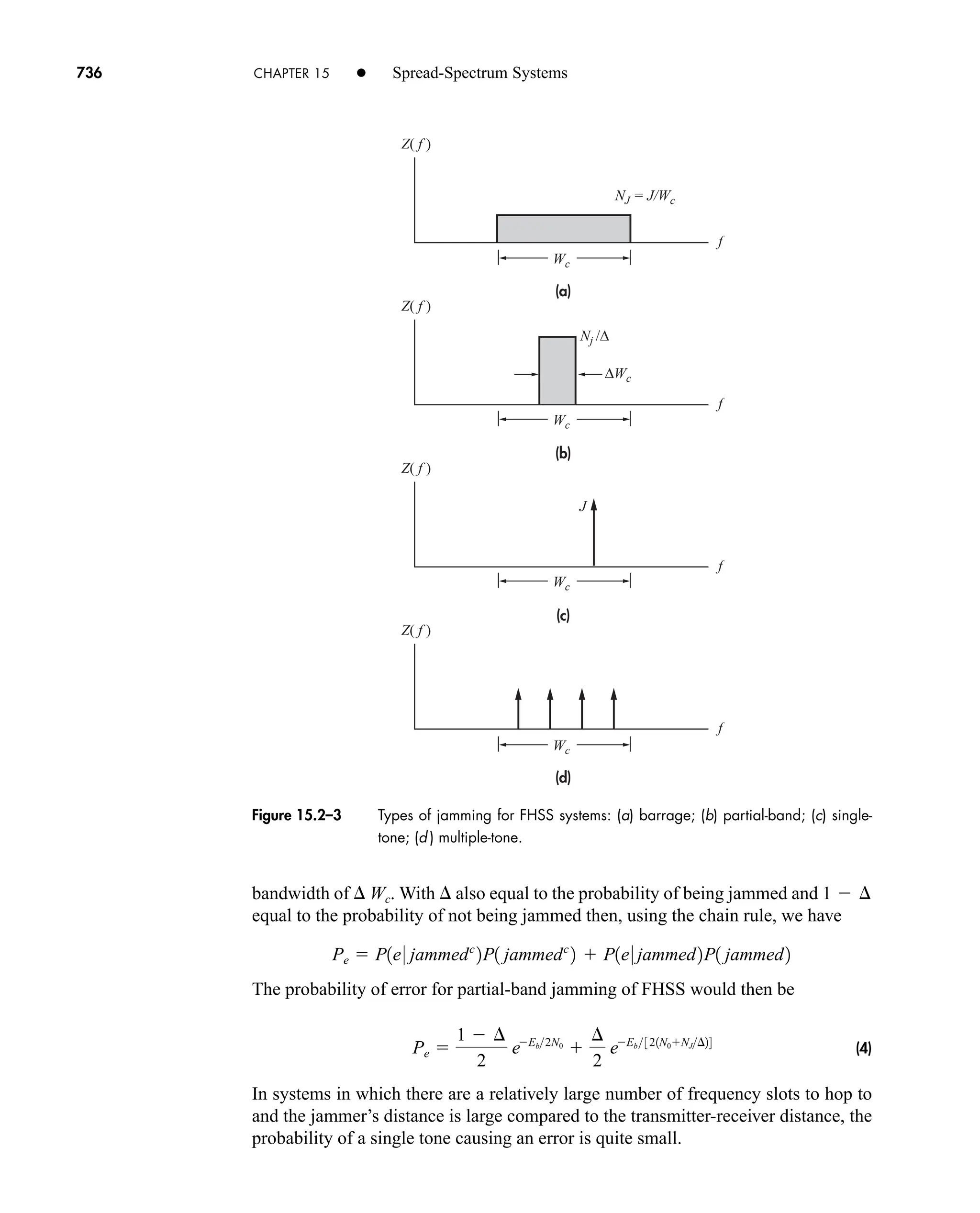
resented by
(1)
where F[x(t)] stands for the functional relationship between input and output. The
linear property means that Eq. (1) obeys the principle of superposition. Thus, if
(2a)
where are constants, then
(2b)
The time-invariance property means that the system’s characteristics remain fixed
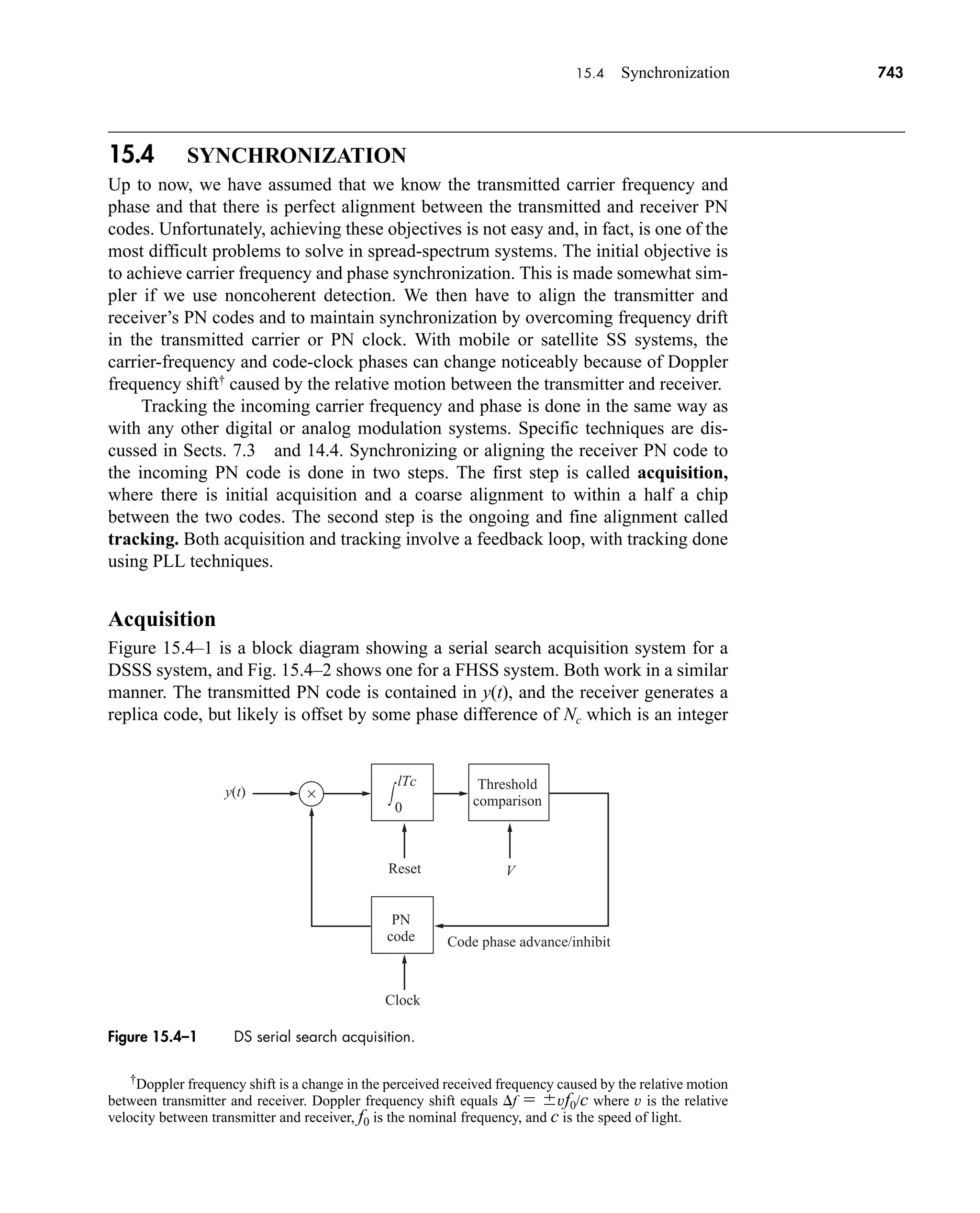
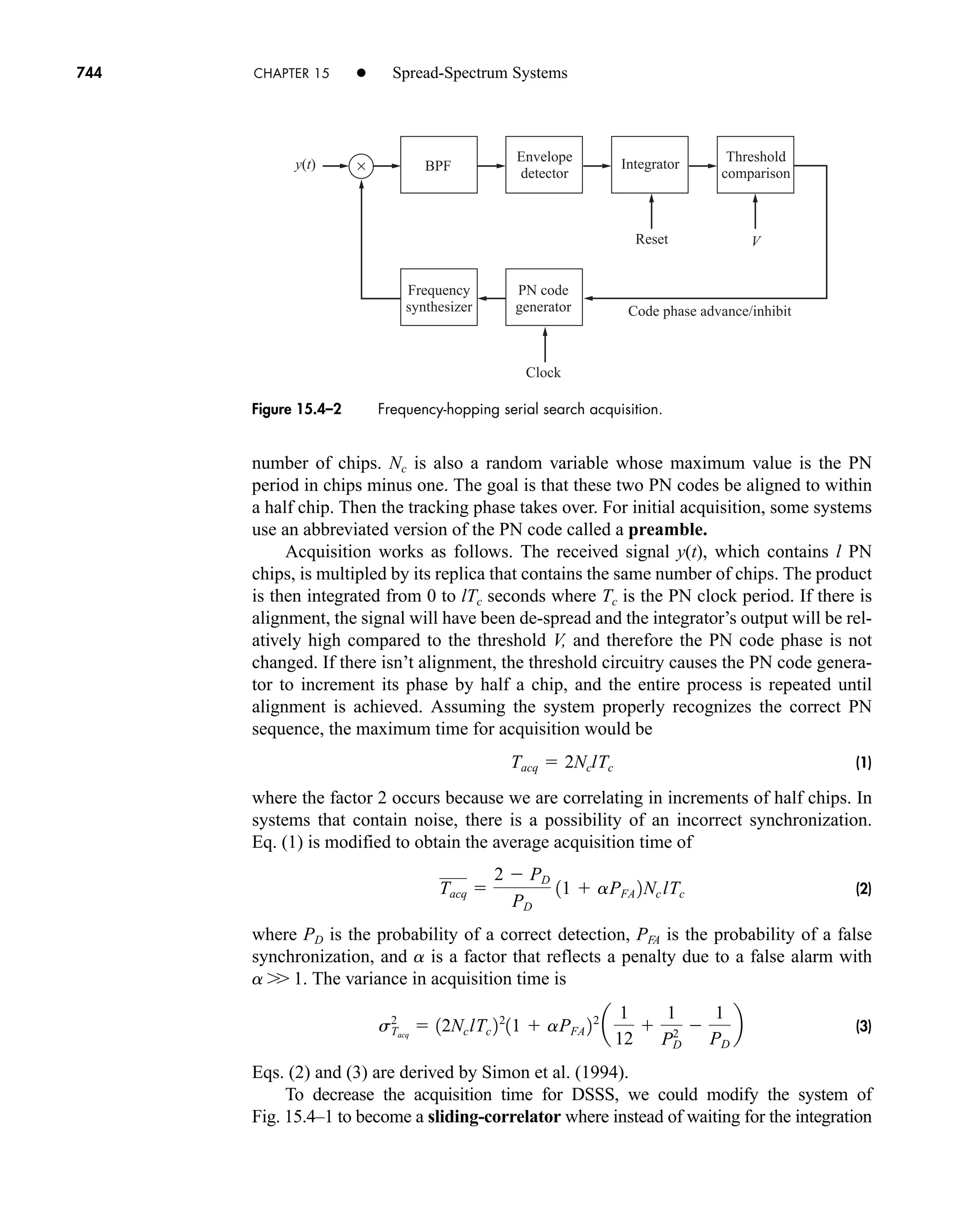
with time. Thus, a time-shifted input produces
(3)
so the output is time-shifted but otherwise unchanged.
Most LTI systems consist entirely of lumped-parameter elements (such as resis-
tors capacitors, and inductors), as distinguished from elements with spatially distrib-
uted phenomena (such as transmission lines). Direct analysis of a lumped-parameter
system starting with the element equations leads to the input–output relation as a
linear differential equation in the form
(4)
an
dn
y1t2
dtn p a1
dy1t2
dt
a0 y1t2 bm
dm
x1t2
dtm p b1
dx1t2
dt
b0 x1t2
F3x1t td 2 4 y1t td 2
x1t td 2
y1t2 a
k
ak F3xk1t2 4
ak
x1t2 a
k
ak xk1t2
y1t2 F3x1t2 4
car80407_ch03_091-160.qxd 12/8/08 11:15 PM Page 93](https://image.slidesharecdn.com/communicationsystemsanintro-a-241115060943-61721fa8/75/Communication_Systems__An_Intro_-_A-_Bruce_Carlson_-pdf-115-2048.jpg)
![94 CHAPTER 3 • Signal Transmission and Filtering
where the a’s and b’s are constant coefficients involving the element values. The
number of independent energy-storage elements determines the value of n, known as
the order of the system. Unfortunately, Eq. (4) doesn’t provide us with a direct ex-
pression for y(t).
To obtain an explicit input–output equation, we must first define the system’s
impulse response function
(5)
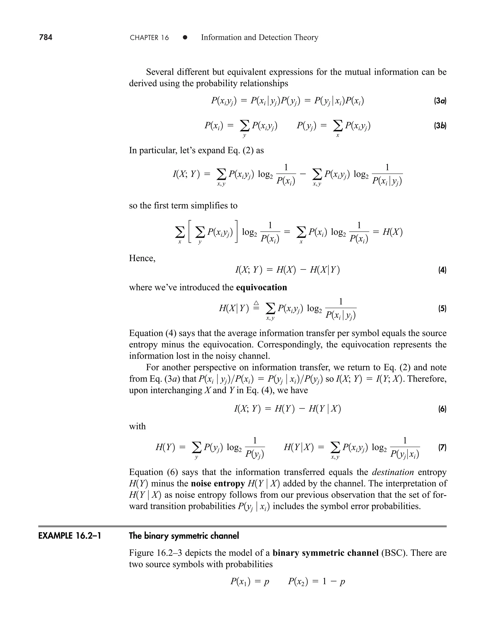
which equals the forced response when . Now any continuous input sig-
nal can be written as the convolution , so
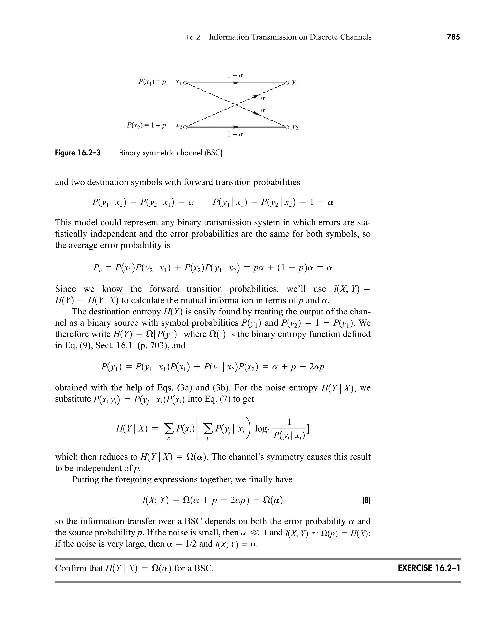
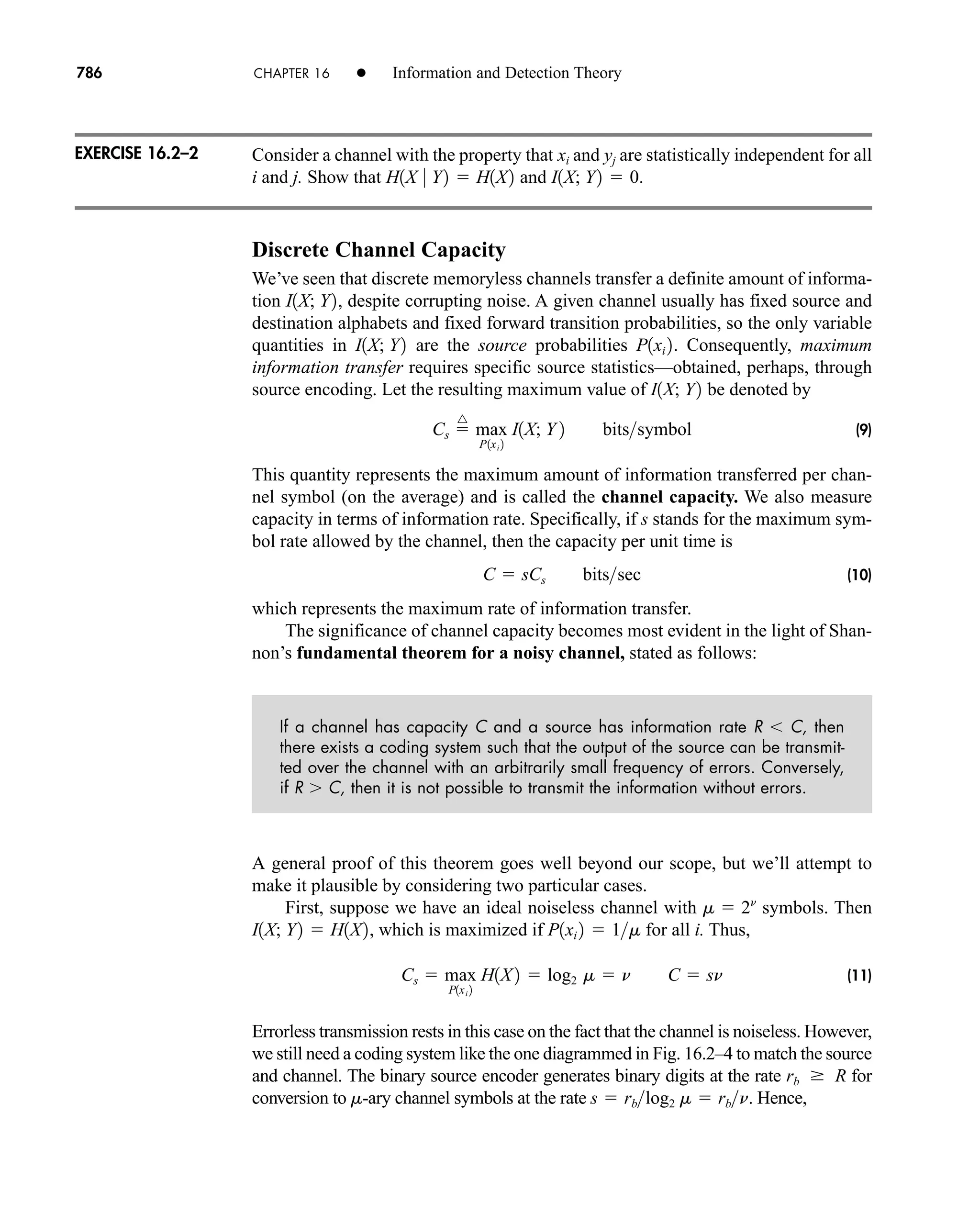
in which the interchange of operations is allowed by virtue of the system’s linearity.
Now, from the time-invariance property, and hence
(6a)
(6b)
where we have drawn upon the commutativity of convolution.
Either form of Eq. (6) is called the superposition integral. It expresses the
forced response as a convolution of the input x(t) with the impulse response h(t).
System analysis in the time domain therefore requires knowledge of the impulse
response along with the ability to carry out the convolution.
Various techniques exist for determining h(t) from a differential equation or some other
system model. However, you may be more comfortable taking and calculating
the system’s step response
(7a)
from which
(7b)
This derivative relation between the impulse and step response follows from the gen-
eral convolution property
Thus, since g(t) h(t) * u(t) by definition, dg(t)/dt h(t) * [du(t)/dt] h(t) * d (t) h(t).
d
dt
3v1t2 * w1t2 4 v1t2 * c
dw1t2
dt
d
h1t2
dg1t2
dt
g1t2
^
F3u1t2 4
x1t2 u1t2
q
q
h1l2x1t l2 dl
y1t2
q
q
x1l2h1t l2 dl
F3d1t l2 4 h1t l2
q
q
x1l2F3d1t l2 4 dl
y1t2 F c
q
q
x1l2d1t l2 dld
x1t2 x1t2 * d1t2
x1t2 d1t2
h1t2
^
F3d1t2 4
car80407_ch03_091-160.qxd 12/8/08 11:15 PM Page 94](https://image.slidesharecdn.com/communicationsystemsanintro-a-241115060943-61721fa8/75/Communication_Systems__An_Intro_-_A-_Bruce_Carlson_-pdf-116-2048.jpg)
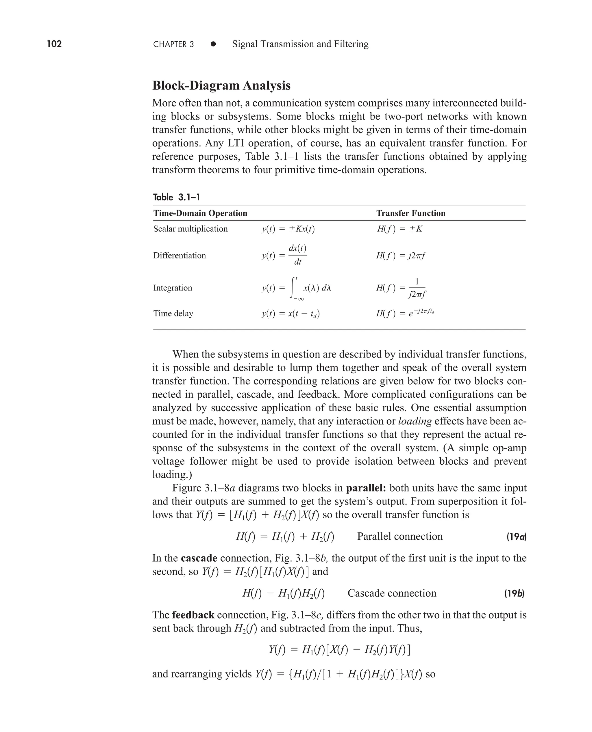
![3.1 Response of LTI Systems 103
Figure 3.1–8 (a) Parallel connection; (b) cascade connection; (c) feedback connection.
(19c)
This case is more properly termed the negative feedback connection as distinguished
from positive feedback, where the returned signal is added to the input instead of
subtracted.
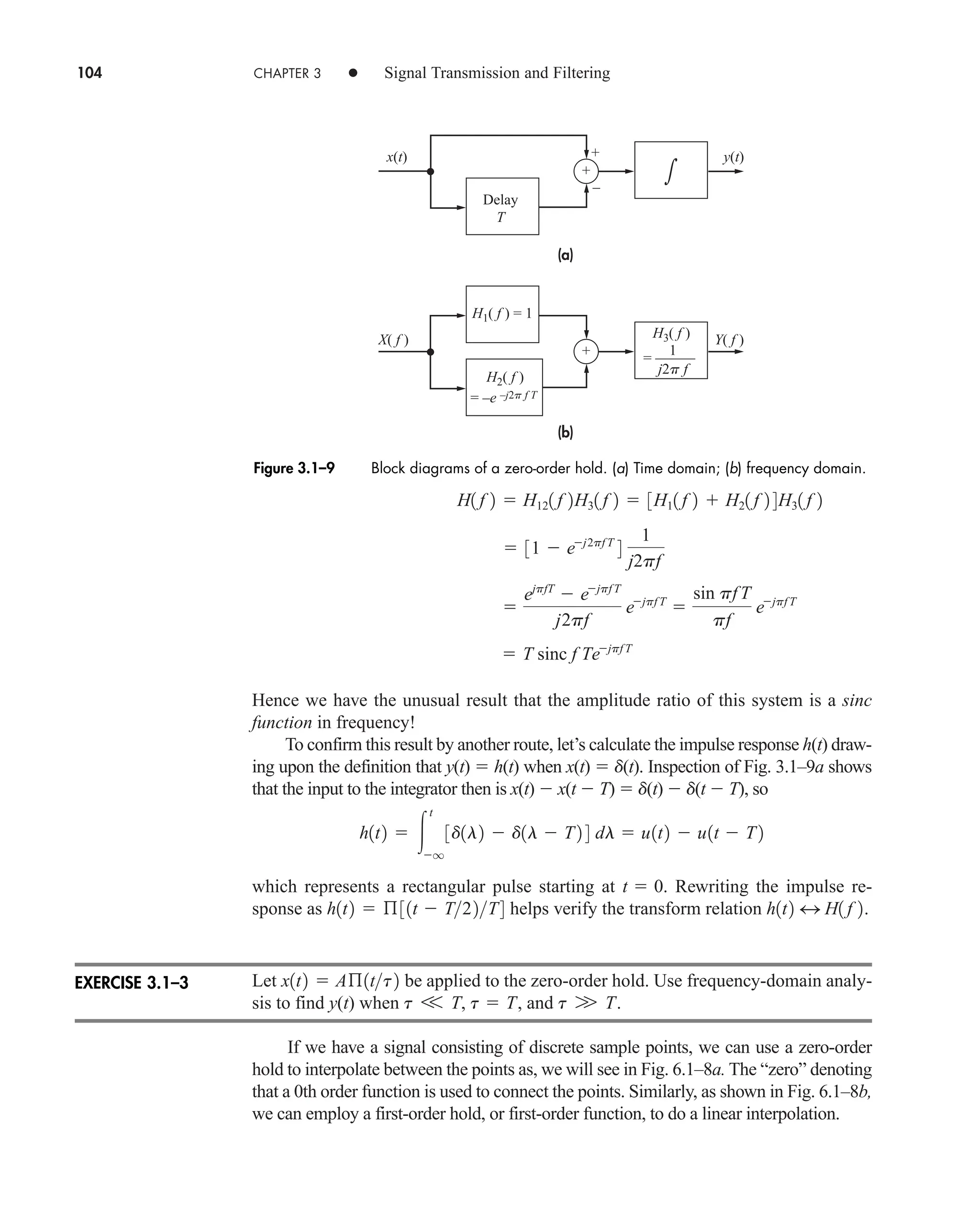
Zero-Order Hold
The zero-order hold system in Fig. 3.1–9a has several applications in electrical com-
munication. Here we take it as an instructive exercise of the parallel and cascade re-
lations. But first we need the individual transfer functions, determined as follows:
the upper branch of the parallel section is a straight-through path so, trivially,
; the lower branch produces pure time delay of T seconds followed by
sign inversion, and lumping them together gives ; the integrator in
the final block has . Figure 3.1–9b is the equivalent block diagram
in terms of these transfer functions.
Having gotten this far, the rest of the work is easy. We combine the parallel
branches in and use the cascade rule to obtain
H121 f 2 H11 f 2 H21 f 2
H31 f 2 1j2pf
H21 f 2 ej2pfT
H11 f 2 1
H1f2
H11f2
1 H11f2H21f2
Feedback connection
+
–
(a)
(b)
(c)
+
+
H1( f )
H1( f ) X( f )
H2( f ) X( f )
H1( f ) X( f )
H2( f ) Y( f )
H1( f )
Y( f ) = [H1( f ) + H2( f )] X( f )
1 + H1( f )H2( f )
Y( f ) = ––––––––––––––––– X( f )
Y( f ) = H1( f )H2( f ) X( f )
X( f )
X( f )
X( f )
H1( f ) H2( f )
H2( f )
H1( f )
H2( f )
EXAMPLE 3.1–3
car80407_ch03_091-160.qxd 12/8/08 11:15 PM Page 103](https://image.slidesharecdn.com/communicationsystemsanintro-a-241115060943-61721fa8/75/Communication_Systems__An_Intro_-_A-_Bruce_Carlson_-pdf-125-2048.jpg)
![114 CHAPTER 3 • Signal Transmission and Filtering
We’ll consider only memoryless devices, for which the transfer characteristic is a
complete description. It should be noted that the transfer function is a purely linear
concept and is only relevant in linear or linearized systems.
Under small-signal input conditions, it may be possible to linearize the transfer
characteristic in a piecewise fashion, as shown by the thin lines in the figure. The
more general approach is a polynomial approximation to the curve, of the form
(12a)
and the higher powers of x(t) in this equation give rise to the nonlinear distortion.
Even though we have no transfer function, the output spectrum can be found, at least
in a formal way, by transforming Eq. (12a). Specifically, invoking the convolution theorem,
(12b)
Now if x(t) is bandlimited in W, the output of a linear network will contain no fre-
quencies beyond But in the nonlinear case, we see that the output includes
, which is bandlimited in , which is bandlimited in ,
and so on. The nonlinearities have therefore created output frequency components
that were not present in the input. Furthermore, since may contain compo-
nents for this portion of the spectrum overlaps that of . Using filtering
techniques, the added components at can be removed, but there is no con-
venient way to get rid of the added components at These, in fact, constitute
the nonlinear distortion.
A quantitative measure of nonlinear distortion is provided by taking a simple co-
sine wave, , as the input. Inserting in Eq. (12a) and expanding yields
a
a2
2
a4
4
pb cos 2v0t p
y1t2 a
a2
2
3a4
8
pb aa1
3a3
4
pb cos v0t
x1t2 cos v0t
f 6 W.
f 7 W
X1 f 2
f 6 W,
X * X1 f 2
3W
2W, X * X * X1 f 2
X * X1 f 2
f 6 W.
Y1 f 2 a1 X1 f 2 a2 X * X1 f 2 a3 X * X * X1 f 2 p
y1t2 a1 x1t2 a2 x2
1t2 a3 x3
1t2 p
x
y = T[x]
Figure 3.2–10 Transfer characteristic of a nonlinear device.
car80407_ch03_091-160.qxd 12/8/08 11:15 PM Page 114](https://image.slidesharecdn.com/communicationsystemsanintro-a-241115060943-61721fa8/75/Communication_Systems__An_Intro_-_A-_Bruce_Carlson_-pdf-136-2048.jpg)
![3.2 Signal Distortion in Transmission 115
Therefore, the nonlinear distortion appears as harmonics of the input wave. The
amount of second-harmonic distortion is the ratio of the amplitude of this term to
that of the fundamental, or in percent:
Higher-order harmonics are treated similarly. However, their effect is usually much
less, and many can be removed entirely by filtering.
If the input is a sum of two cosine waves, say cos , the output will
include all the harmonics of f1 and f2, plus crossproduct terms which yield
f2 f1, f2 f1, f2 2f1, etc. These sum and difference frequencies are designated as
intermodulation distortion. Generalizing the intermodulation effect, if x(t) x1(t) x2(t),
then y(t) contains the cross-product x1(t)x2(t) (and higher-order products, which we ignore
here). In the frequency domain x1(t)x2(t) becomes X1 * X2(f); and even though X1(f)
and X2(f) may be separated in frequency, X1 * X2(f) can overlap both of them, pro-
ducing one form of crosstalk. Note that nonlinearity is not required for other forms
of crosstalk (e.g., signals traveling over adjacent cables can have crosstalk). This as-
pect of nonlinear distortion is of particular concern in telephone transmission sys-
tems. On the other hand the cross-product term is the desired result when nonlinear
devices are used for modulation purposes.
It is important to note the difference between crosstalk and other types of inter-
ference. Crosstalk occurs when one signal crosses over to the frequency band of an-
other signal due to nonlinear distortion in the channel. Picking up a conversation on
a cordless phone or baby monitor occurs because the frequency spectrum allocated
to such devices is too crowded to accommodate all of the users on separate frequen-
cy carriers. Therefore some “sharing” may occur from time to time. While crosstalk
resulting from nonlinear distortion is now rare in telephone transmission due to ad-
vances in technology, it was a major problem at one time.
The cross-product term is the desired result when nonlinear devices are used for
modulation purposes. In Sect. 4.3 we will examine how nonlinear devices can be
used to achieve amplitude modulation. In Chap. 5, carefully controlled nonlinear dis-
tortion again appears in both modulation and detection of FM signals.
Although nonlinear distortion has no perfect cure, it can be minimized by care-
ful design. The basic idea is to make sure that the signal does not exceed the linear
operating range of the channel’s transfer characteristic. Ironically, one strategy along
this line utilizes two nonlinear signal processors, a compressor at the input and an
expander at the output, as shown in Fig. 3.2–11.
A compressor has greater amplification at low signal levels than at high signal lev-
els, similar to Fig. 3.2–10, and thereby compresses the range of the input signal. If the
compressed signal falls within the linear range of the channel, the signal at the channel
output is proportional to Tcomp[x(t)] which is distorted by the compressor but not the chan-
nel. Ideally, then, the expander has a characteristic that perfectly complements the com-
pressor so the expanded output is proportional to Texp{Tcomp[x(t)]} x(t), as desired.
The joint use of compressing and expanding is called companding (surprise?)
and is of particular value in telephone systems. Besides reducing nonlinear
v1t cos v2t
Second-harmonic distortion `
a22 a44 p
a1 3a34 p ` 100%
car80407_ch03_091-160.qxd 12/8/08 11:15 PM Page 115](https://image.slidesharecdn.com/communicationsystemsanintro-a-241115060943-61721fa8/75/Communication_Systems__An_Intro_-_A-_Bruce_Carlson_-pdf-137-2048.jpg)
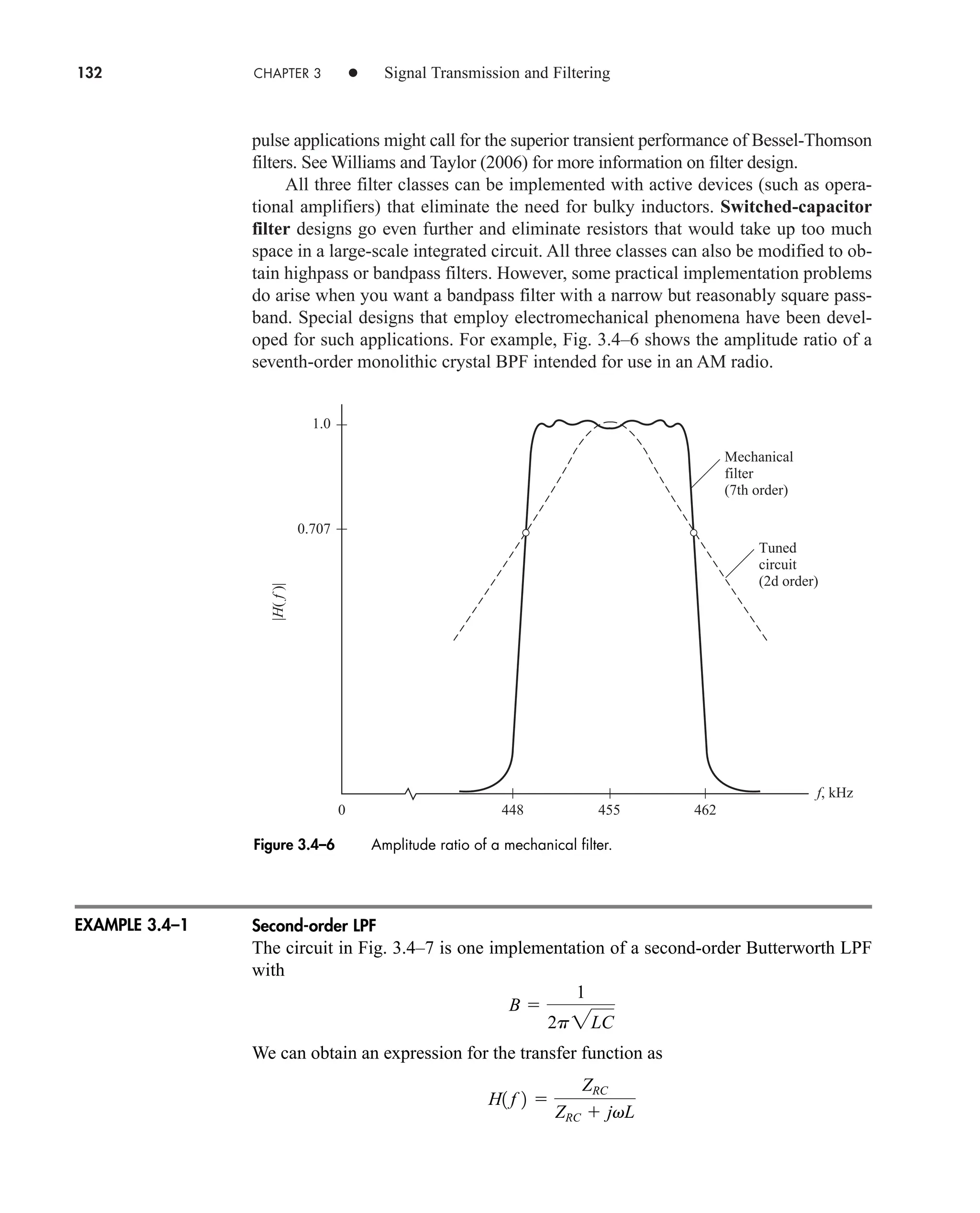
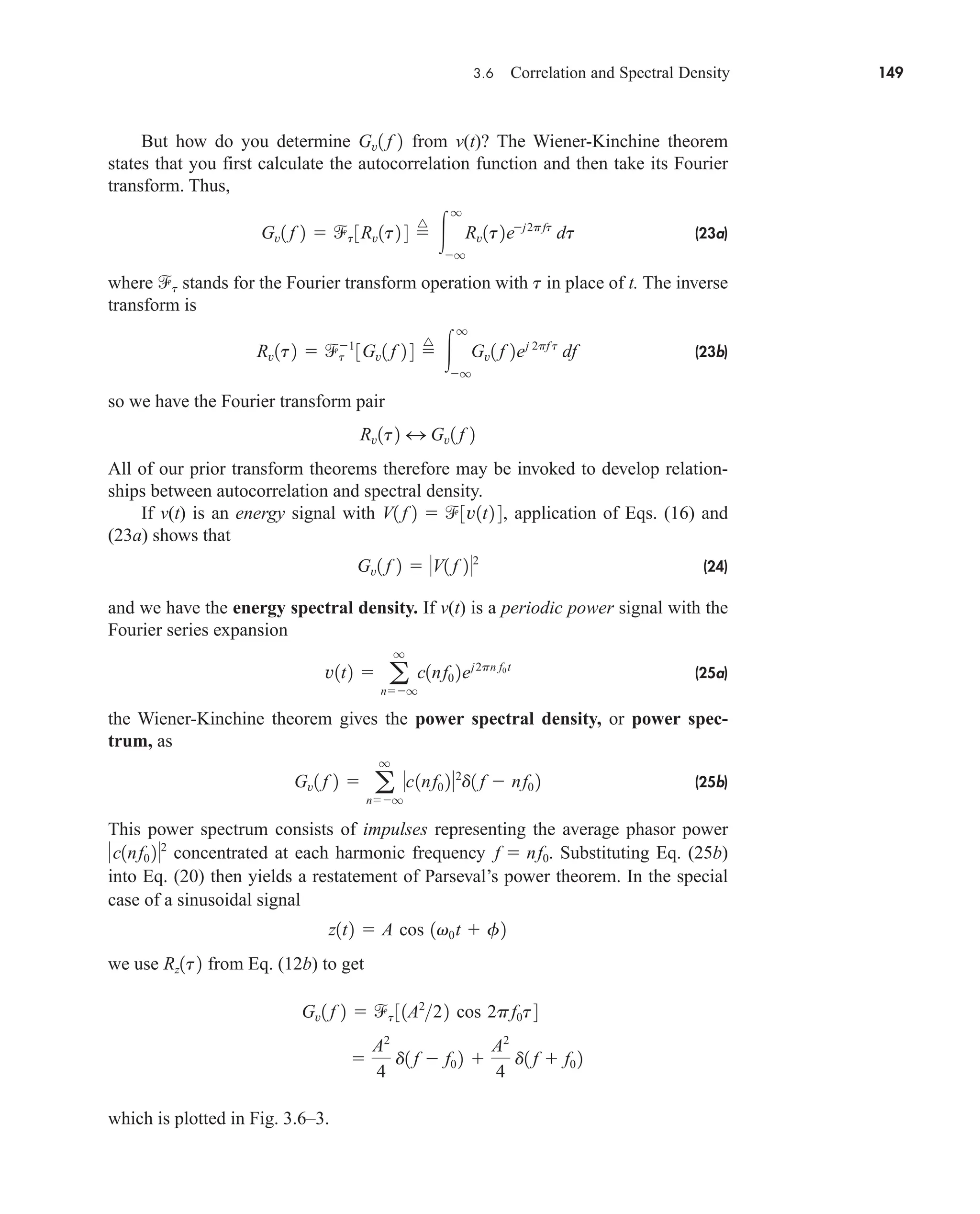
![146 CHAPTER 3 • Signal Transmission and Filtering
Pattern Recognition
Cross-correlation can be used in pattern recognition tasks. If the cross-correlation of ob-
jects A and B is similar to the autocorrelation of A, then B is assumed to match A. Oth-
erwise B does not match A. For example, the autocorrelation of x(t) (t) can be
found from performing the graphical correlation in Eq. (14b) as Rx(t) (t). If we ex-
amine the similarity of y(t) 2 (t) to x(t) by finding the cross-correlation Rxy(t)
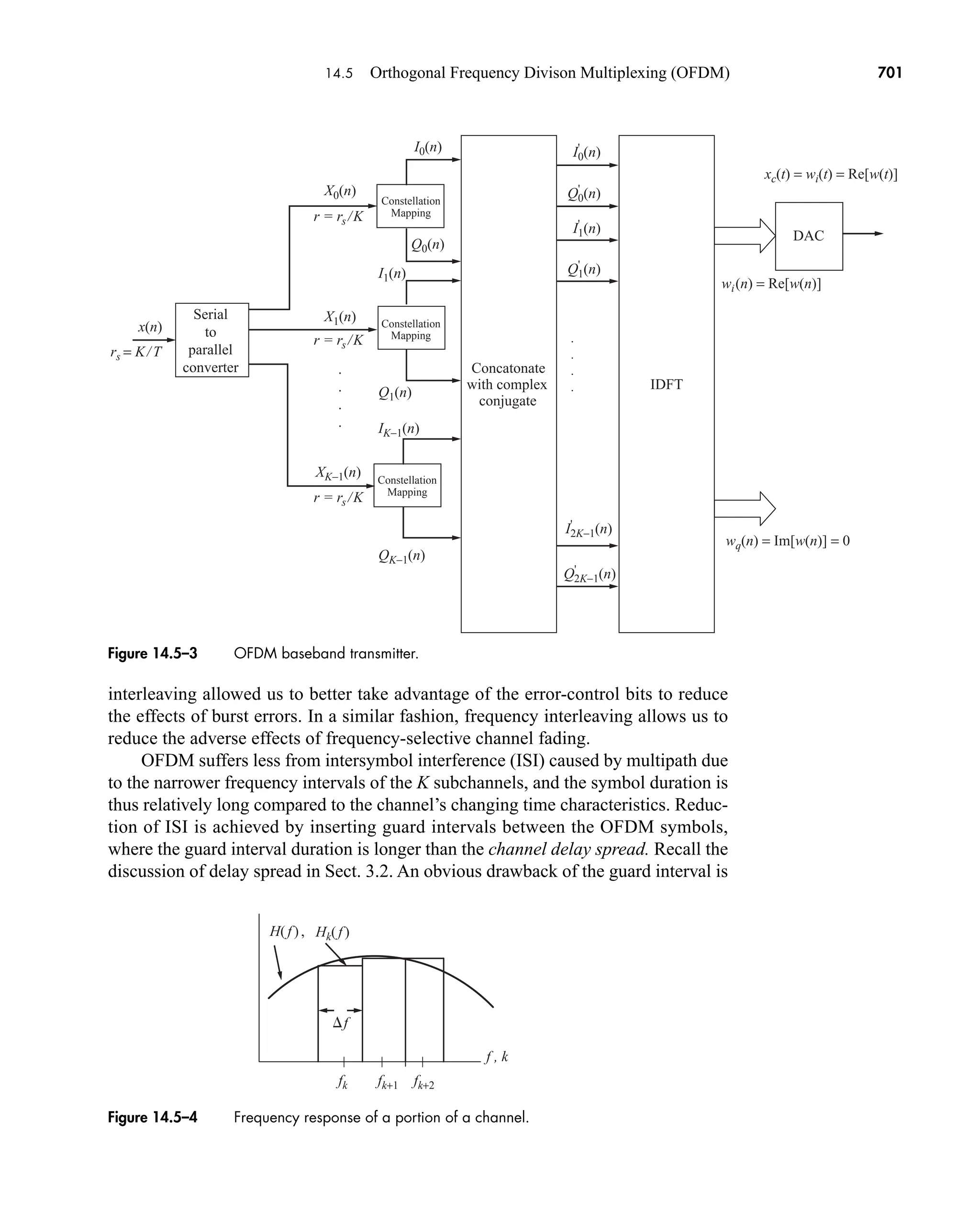
2 (t), we see that Rxy(t) is just a scaled version of Rx(t). Therefore y(t) matches x(t).
However, if we take the cross-correlation of z(t) u(t) with x(t), we obtain
and conclude that z(t) doesn’t match x(t)
This type of graphical correlation is particularly effective for signals that do not
have a closed-form solution. For example, autocorrelation can find the pitch (funda-
mental frequency) of speech signals. The cross-correlation can determine if two speech
samples have the same pitch, and thus may have come from the same individual.
Let v(t) A[u(t) u(t D)] and w(t) v(t td). Use Eq. (16) with z(t) w*(t)
to sketch Rvw(t). Confirm from your sketch that and that
at .
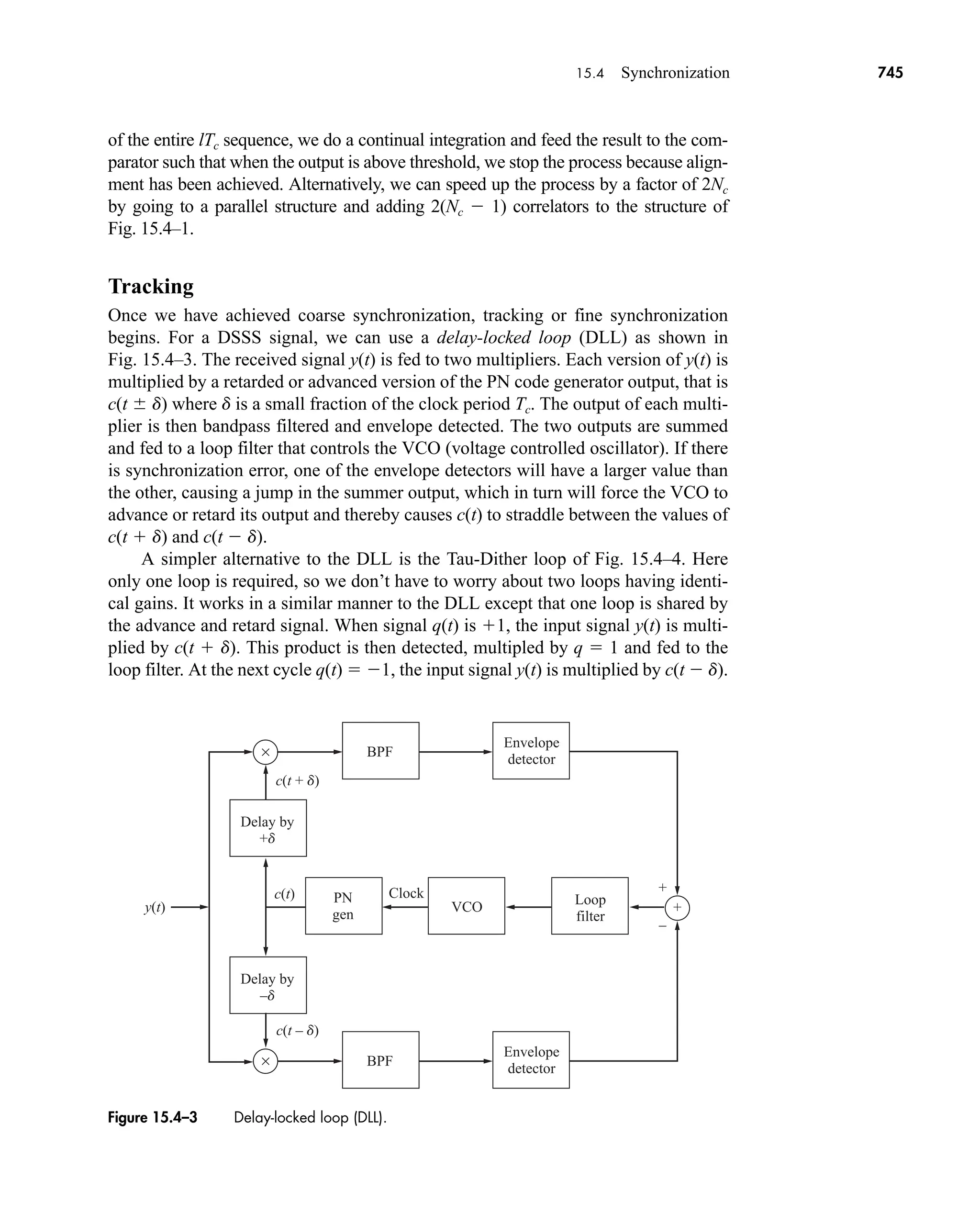
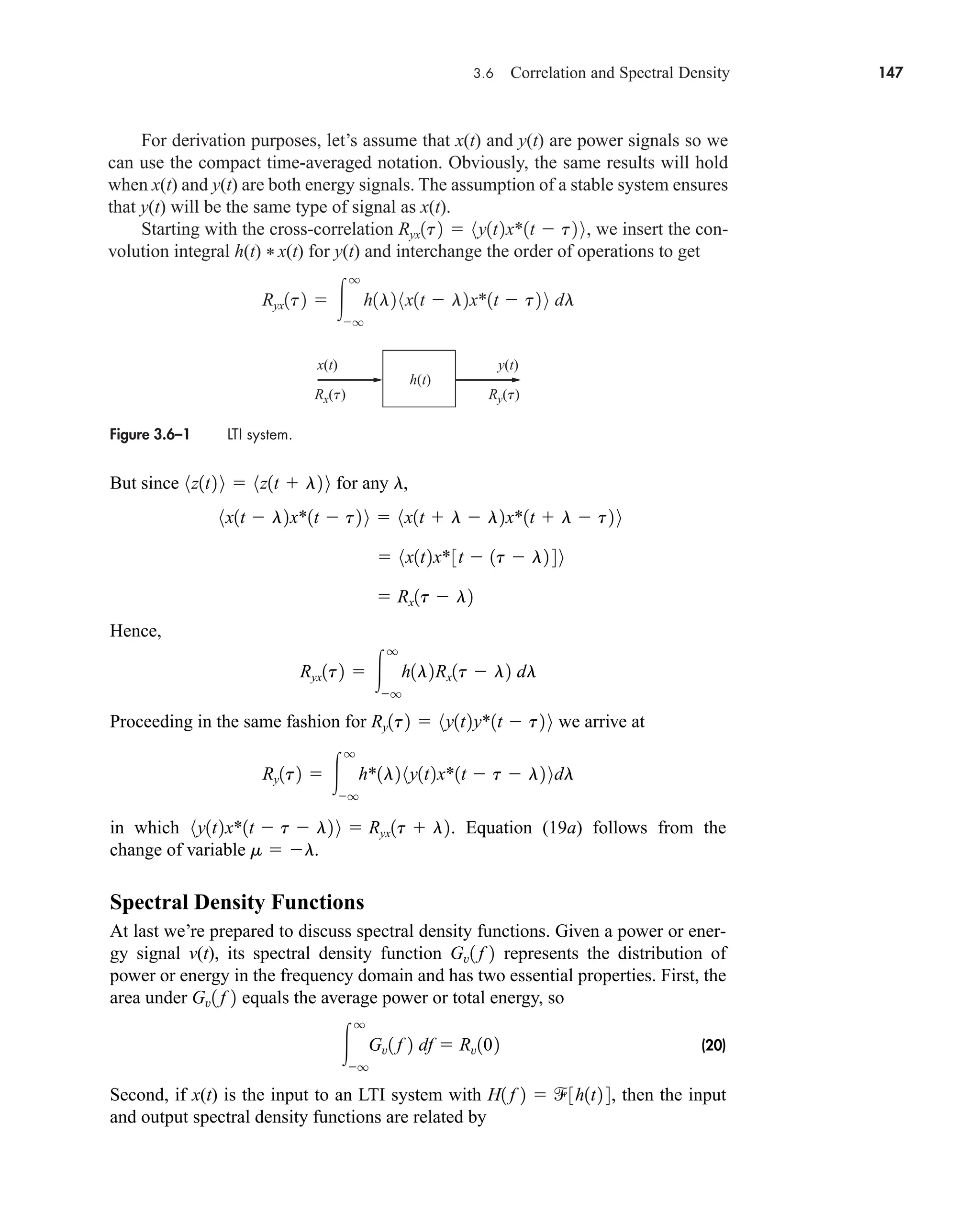
We next investigate system analysis in the “ domain,” as represented by
Fig. 3.6–1. A signal x(t) having known autocorrelation is applied to an LTI sys-
tem with impulse response h(t), producing the output signal
We’ll show that the input-output cross-correlation function is
(18)
and that the output autocorrelation function is
(19a)
Substituting Eq. (18) into (19a) then gives
(19b)
Note that these t-domain relations are convolutions, similar to the time-domain relation.
Ry1t2 h*1t2 * h1t2 * Rx1t2
Ry1t2 h*1t2 * Ryx1t2
q
q
h*1m2Ryx 1t m2 dm
Ryx1t2 h1t2 * Rx1t2
q
q
h1l2 Rx1t l2 dl
y1t2 h1t2 * x1t2
q
q
h1l2 x1t l2 dl
Rx1t2
t
t td
0Rvw1t2 0max
2
EvEw
0Rvw1t2 02
EvEw
Rxz1t2 •
1 for t 6 12
12 t for 12 t 12
0 for t 7 12
EXAMPLE 3.6–2
EXERCISE 3.6–2
car80407_ch03_091-160.qxd 12/8/08 11:15 PM Page 146](https://image.slidesharecdn.com/communicationsystemsanintro-a-241115060943-61721fa8/75/Communication_Systems__An_Intro_-_A-_Bruce_Carlson_-pdf-168-2048.jpg)
![3.7 Questions and Problems 155
Express your answer in the form of y(t) Kx(t td). How does the
phase term affect the output time delays?
3.2–2 Do Prob. 3.2–1 with a system whose frequency response is What
is the effect of nonlinear phase distortion?
3.2–3 Show that a first-order lowpass system yields essentially distortionless
transmission if x(t) is bandlimited to .
3.2–4 Find and sketch y(t) when the test signal
, which approximates a triangular wave, is applied to a first-order
lowpass system with .
3.2–5* Find and sketch y(t) when the test signal from Prob. 3.2–4 is applied to a
first-order highpass system with and .
3.2–6 The signal 2 sinc 40t is to be transmitted over a channel with transfer
function H(f). The output is . Find H(f) and
sketch its magnitude and phase over .
3.2–7 Evaluate at , 0.5, 1, and 2 kHz for a first-order lowpass sys-
tem with kHz.
3.2–8 A channel has the transfer function
Sketch the phase delay and group delay . For what values of f
does ?
3.2–9 Consider a transmission channel with HC(f) (1 2a cos vT)ejvT
, which has
amplitude ripples. (a) Show that , so
theoutputincludesaleadingandtrailingecho.(b)Let and .
Sketch y(t) for and
3.2–10* Consider a transmission channel with HC(f ) exp[j(vT a sin vT)],
which has phase ripples. Assume and use a series expansion
to show that the output includes a leading and trailing echo.
3.2–11 Design a tapped-delay line equalizer for in Prob. 3.2–10 with
.
3.2–12 Design a tapped-delay line equalizer for in Prob. 3.2–9 with
.
3.2–13 Supposex(t)Acosv0tisappliedtoanonlinearsystemwithy(t)2x(t)–3x3
(t).
Write y(t) as a sum of cosines. Then evaluate the second-harmonic and third-
harmonic distortion when and .
A 2
A 1
a 0.4
Hc1 f 2
a 0.4
Hc1 f 2
a V p2
4T
3 .
t 2T
3
a 1
2
x1t2 ß1tt2
y1t2 ax1t2 x1t T2 ax1t 2T2
td1 f 2 tg1 f 2
tg1 f 2
td1 f 2
H1 f 2 µ
4ß a
f
40
bejpf30
for f 15 Hz
4ß a
f
40
bejp2
for f 7 15 Hz
B 2
f 0
td1 f 2
f 30
y1t2 20 sinc 140t 2002
B 3f0
H1 f 2 jf1B jf 2
B 3f0
4
25 cos 5v0t
x1t2 4 cos v0t 4
9 cos 3v0t
W V B
5ejv2
.
car80407_ch03_091-160.qxd 1/23/09 12:23 PM Page 155
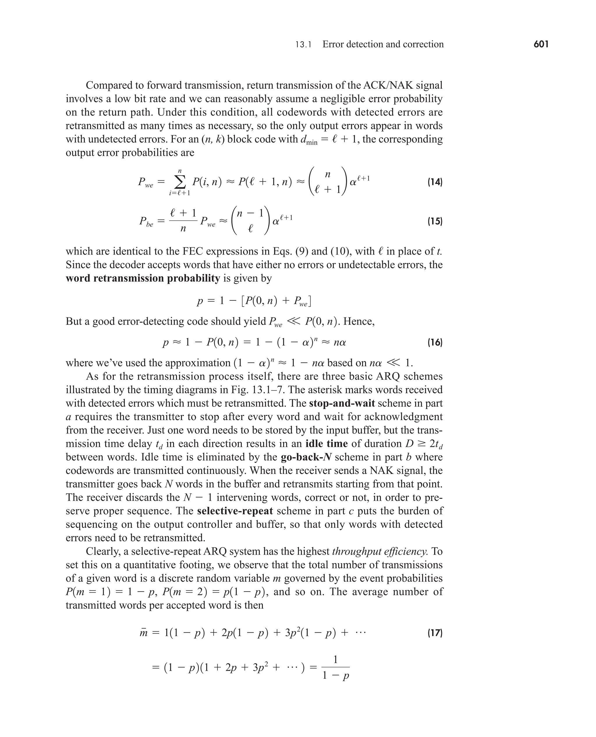
Rev.Confirming Pages](https://image.slidesharecdn.com/communicationsystemsanintro-a-241115060943-61721fa8/75/Communication_Systems__An_Intro_-_A-_Bruce_Carlson_-pdf-177-2048.jpg)

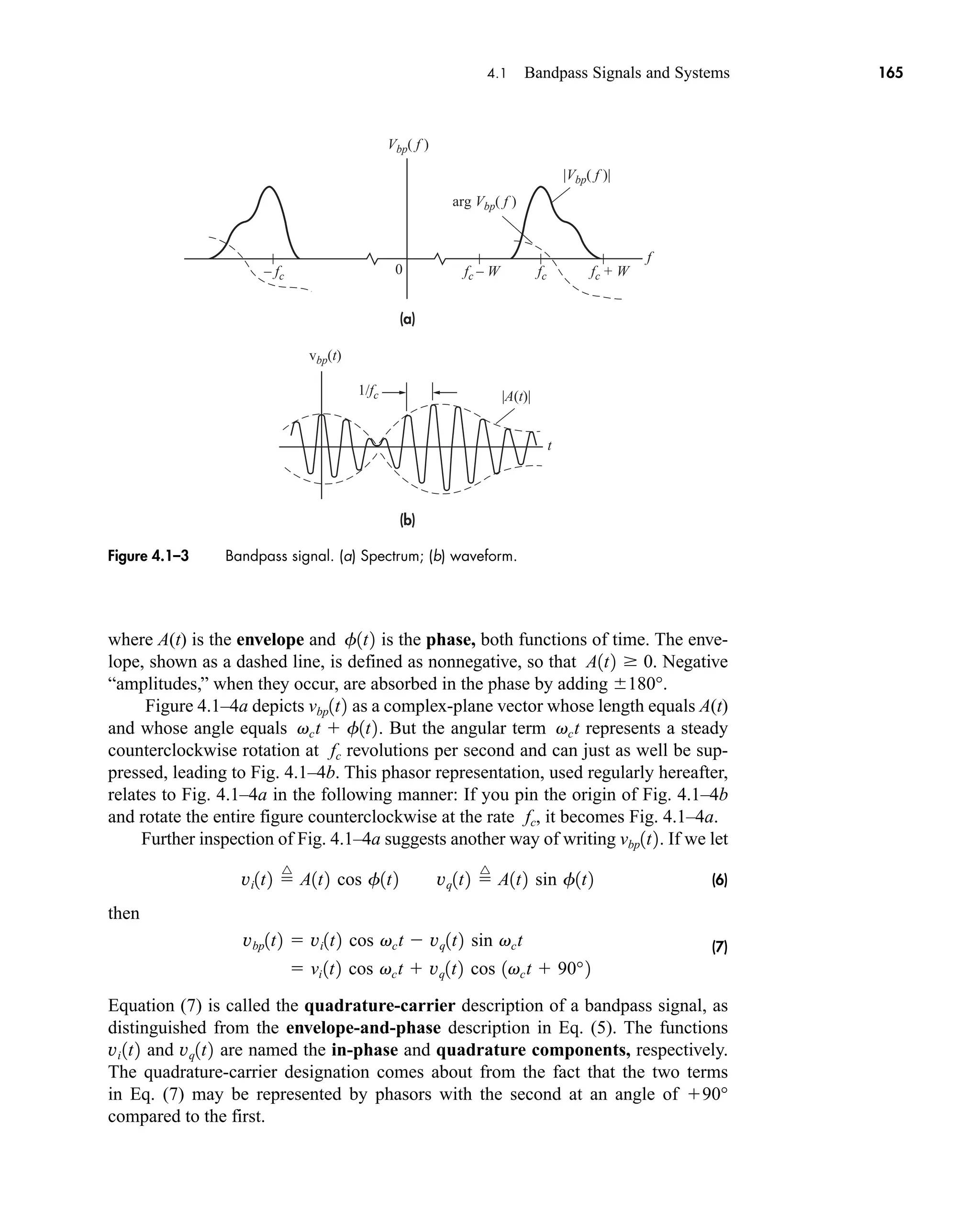
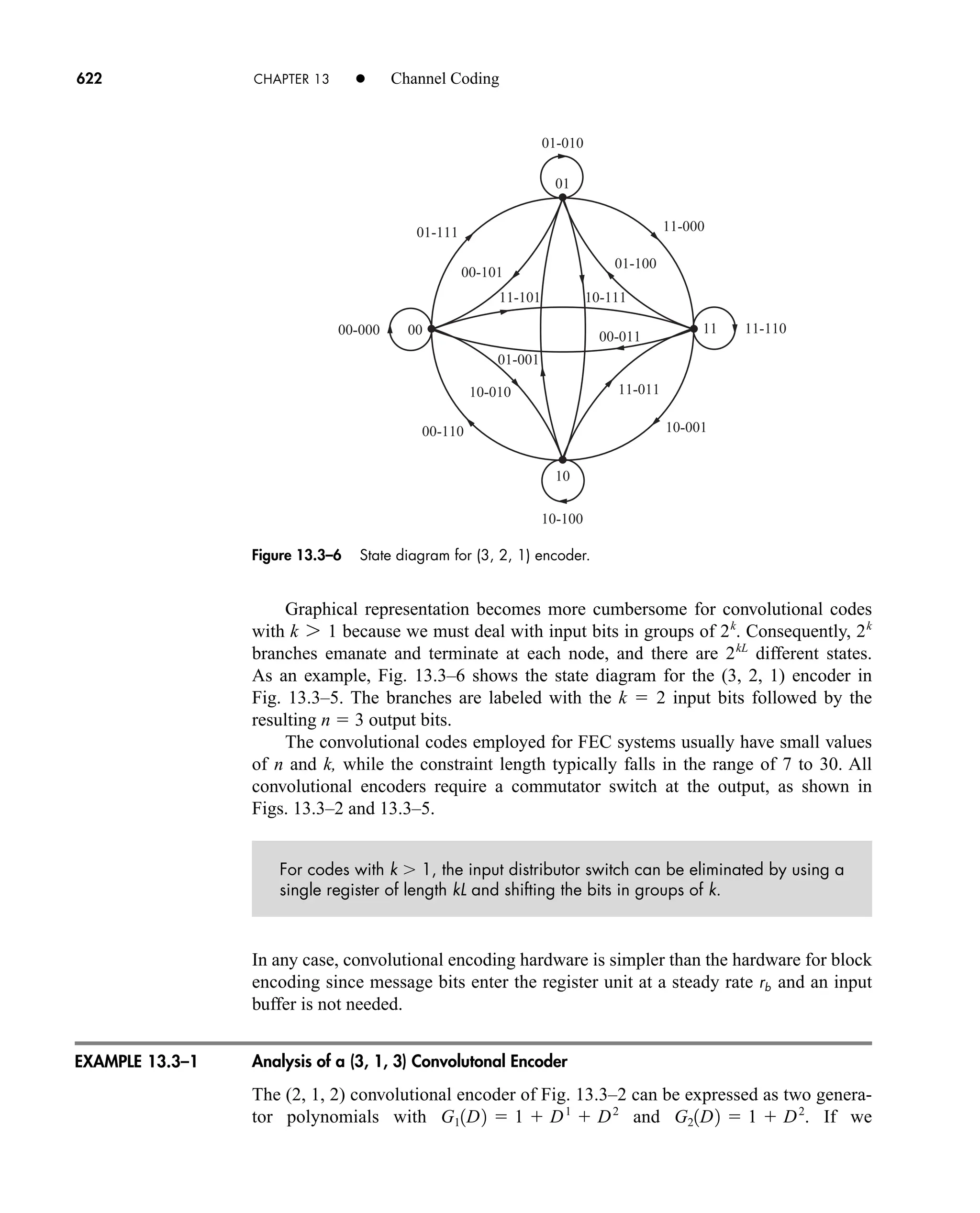
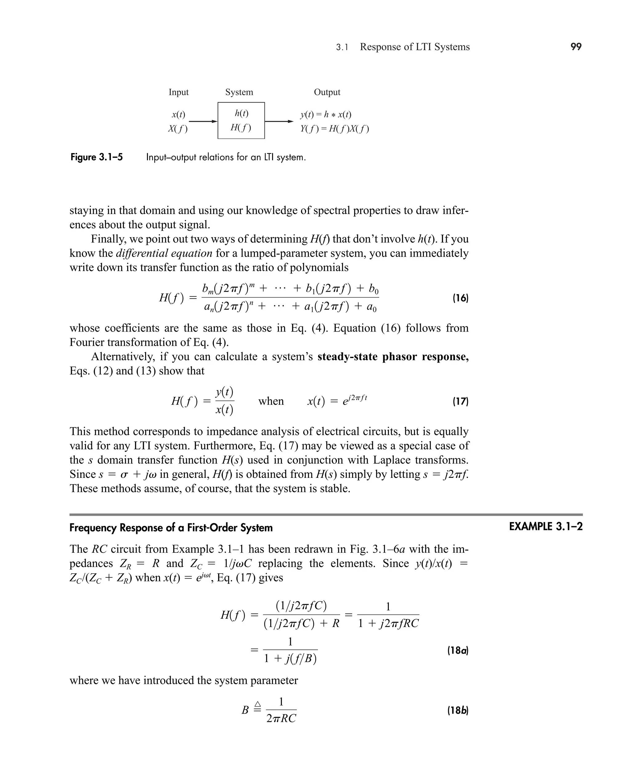
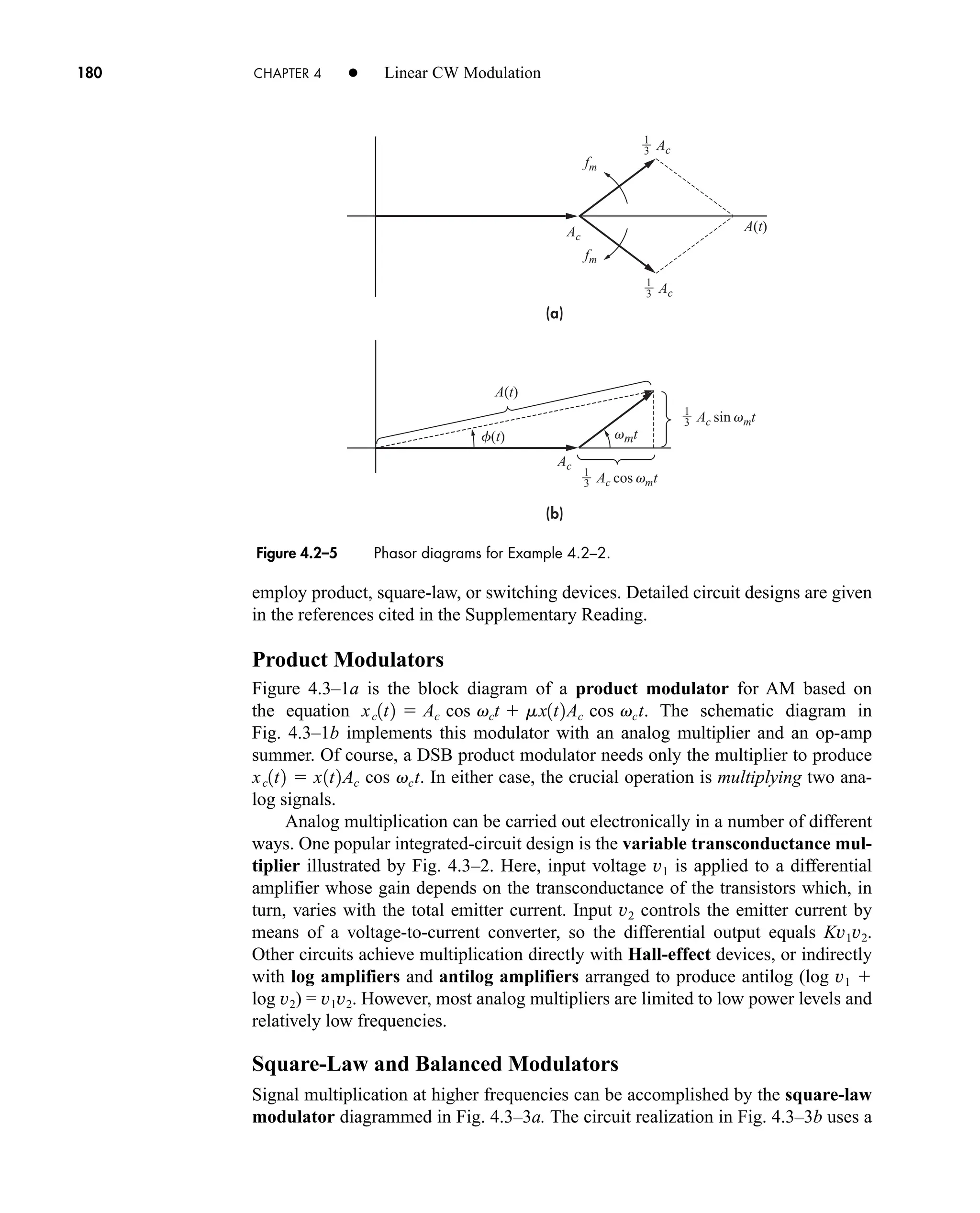
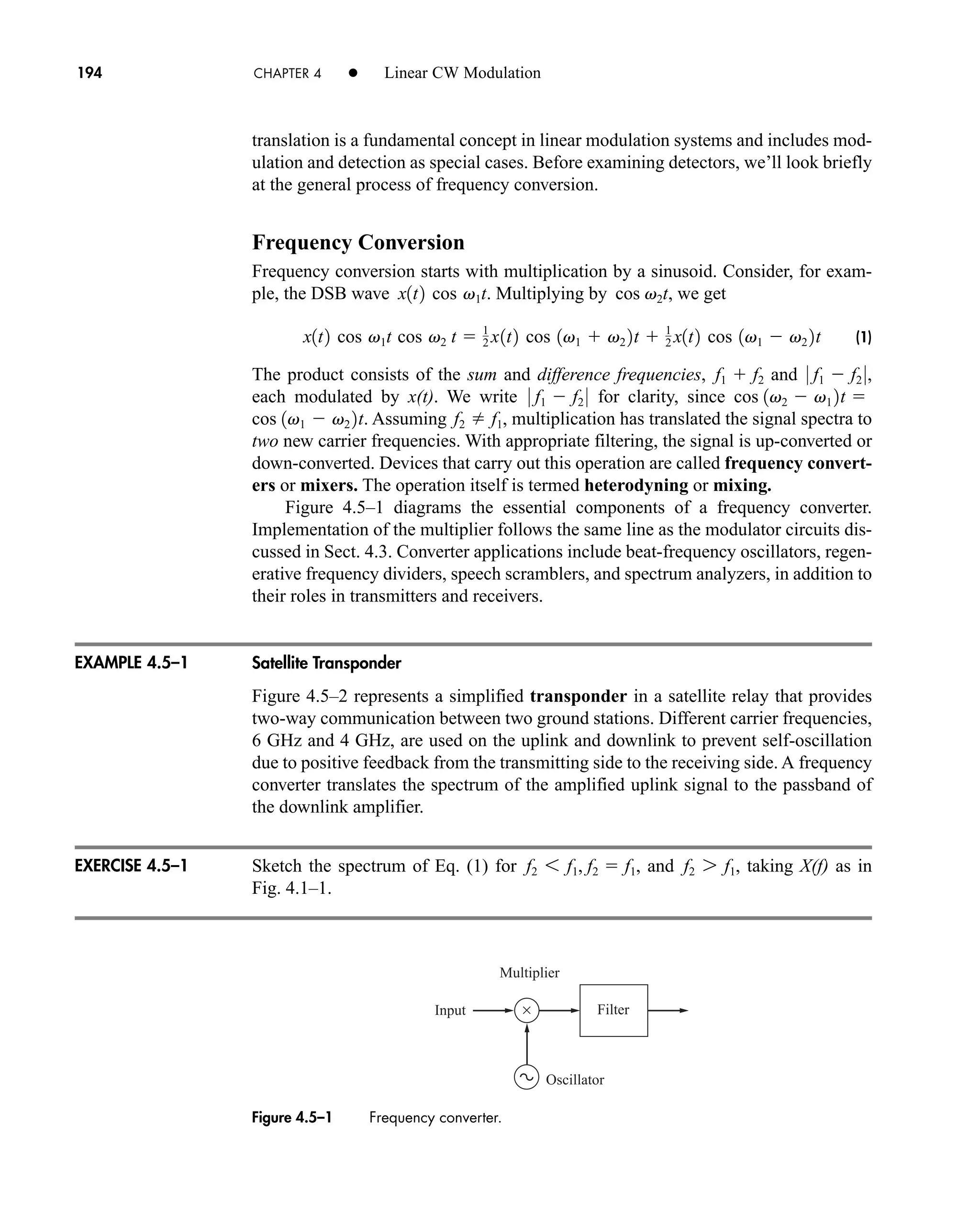
![Figure 4.1–6 (a) Bandpass system; (b) lowpass model.
(a) (b)
xbp(t) ybp(t) xp(t) yp(t)
Hbp( f ) Hp( f )
168 CHAPTER 4 • Linear CW Modulation
bandpass signals, we can keep the hermitian symmetry of in mind and use the
simpler expression
(13b)
which follows from Figs. 4.1–3a and 4.1–5.
Let and use 2 Re [z(t)] = z(t) + z*(t) to derive Eq. (13a) from Eq. (12).
Bandpass Transmission
Now we have the tools needed to analyze bandpass transmission represented by
Fig. 4.1–6a where a bandpass signal applied to a bandpass system with transfer
function produces the bandpass output . Obviously, you could attempt
direct bandpass analysis via . But it’s usually easier to work
with the lowpass equivalent spectra related by
(14a)
where
(14b)
which is the lowpass equivalent transfer function.
Equation (14) permits us to replace a bandpass system with the lowpass equiva-
lent model in Fig. 4.1–6b. Besides simplifying analysis, the lowpass model provides
valuable insight to bandpass phenomena by analogy with known lowpass relation-
ships. We move back and forth between the bandpass and lowpass models with the
help of our previous results for bandpass signals.
In particular, after finding from Eq. (14), you can take its inverse Fourier
transform
The lowpass-to-bandpass transformation in Eq. (12) then yields the output signal
. Or you can get the output quadrature components or envelope and phase
immediately from as
y/p1t2
ybp1t2
y/p1t2 1
3Y/p1 f 2 4 1
3H/p1 f 2X/p1 f 2 4
Y/p1 f 2
H/p1 f 2 Hbp1 f fc 2u1 f fc 2
Y/p1 f 2 H/p1 f 2 X/p1 f 2
Ybp1 f 2 Hbp1 f 2Xbp1 f 2
ybp1t2
Hbp1 f 2
xbp1t2
z1t2 v/p1t2e jvct
Vbp1 f 2 V/p1 f fc 2 f 7 0
Vbp1 f 2
EXERCISE 4.1–1
car80407_ch04_161-206.qxd 1/15/09 4:19 PM Page 168
Rev.Confirming Pages](https://image.slidesharecdn.com/communicationsystemsanintro-a-241115060943-61721fa8/75/Communication_Systems__An_Intro_-_A-_Bruce_Carlson_-pdf-190-2048.jpg)
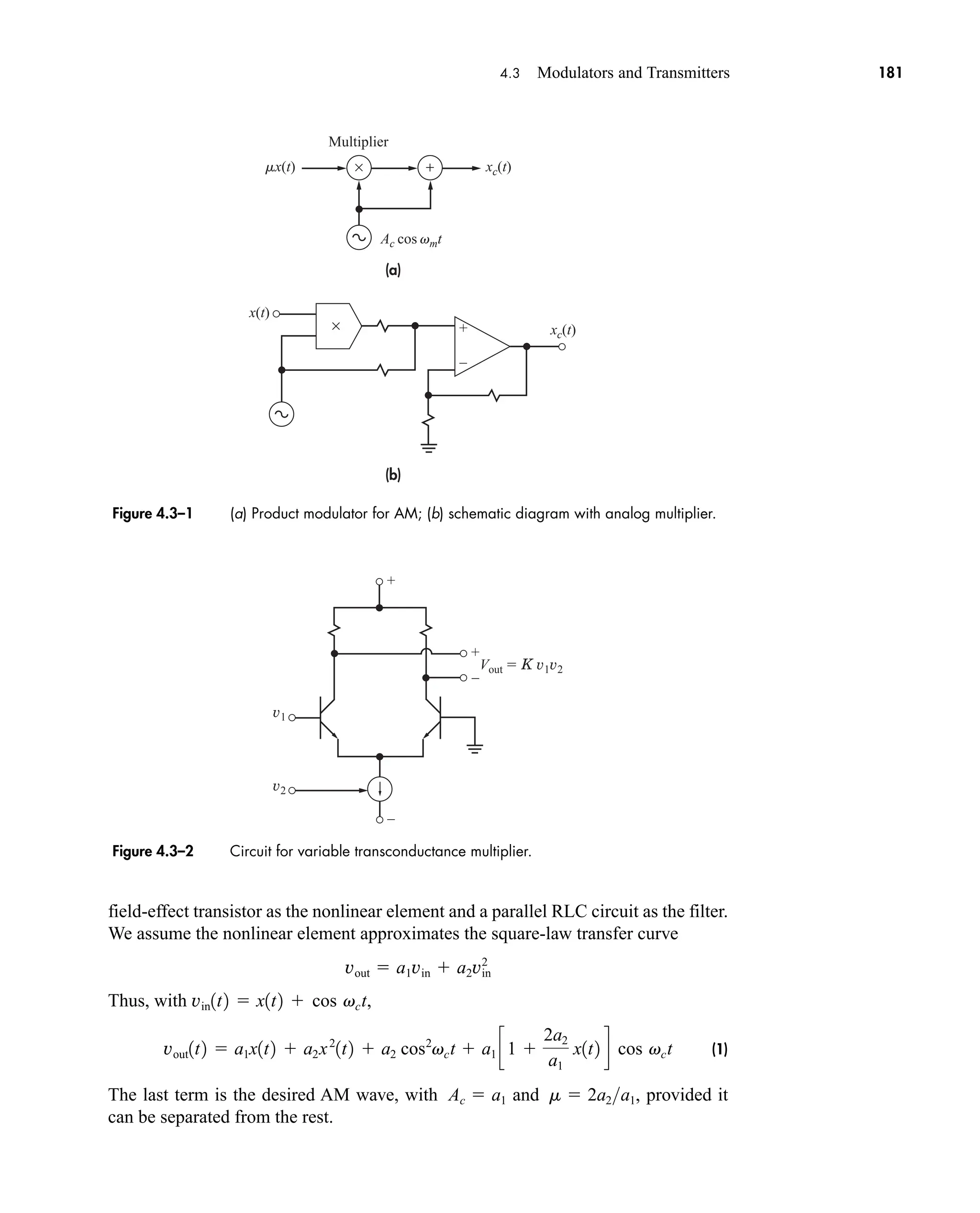
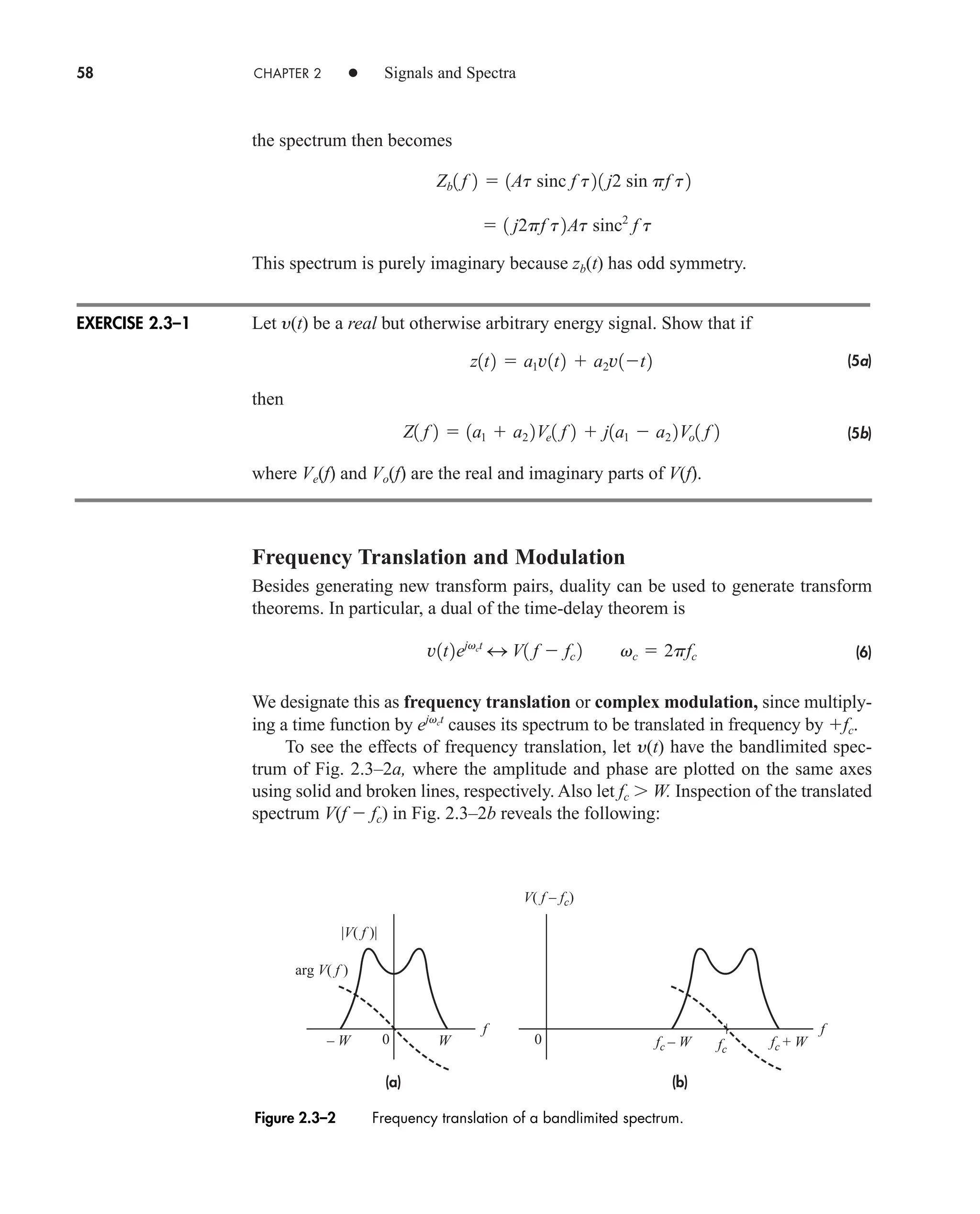
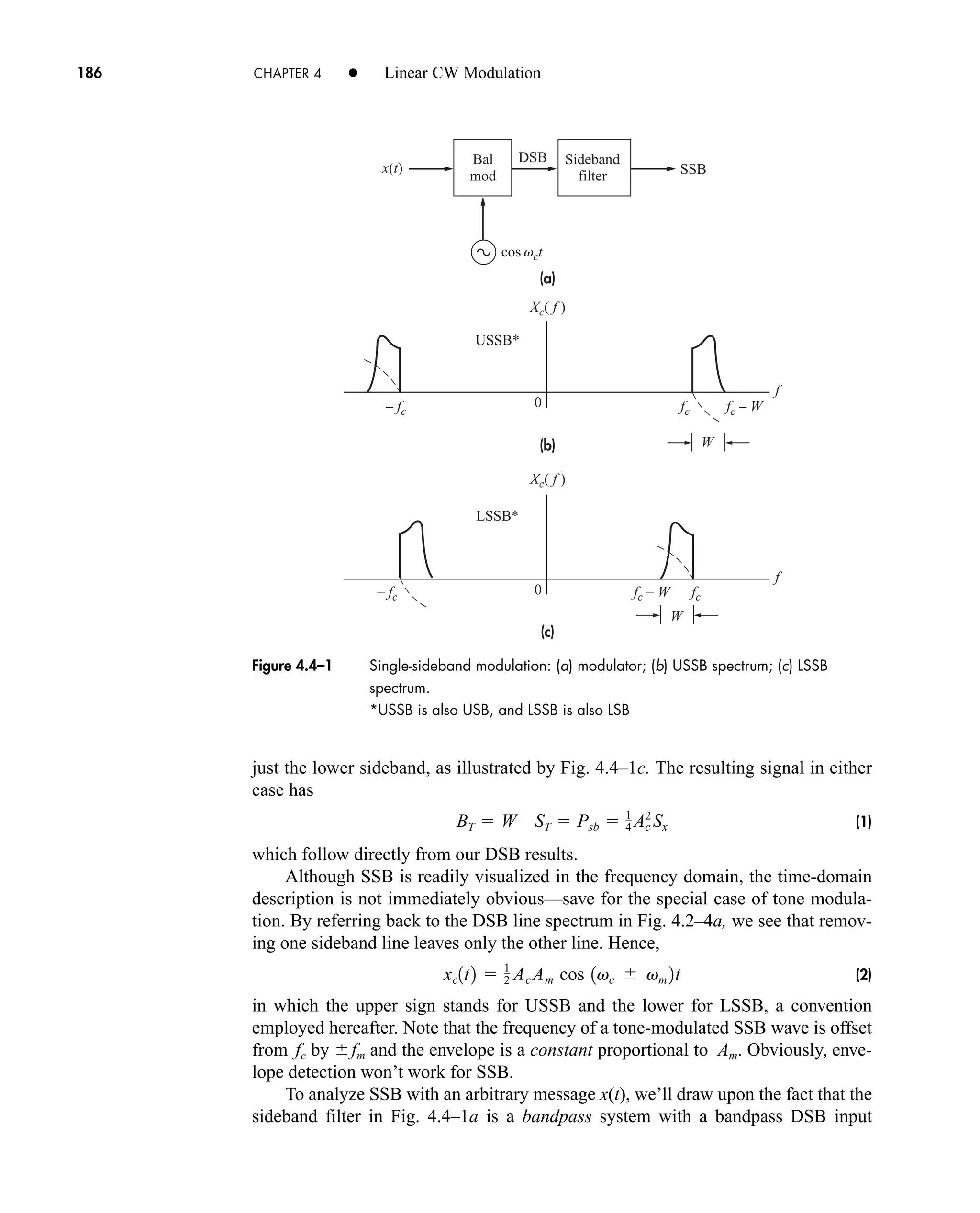
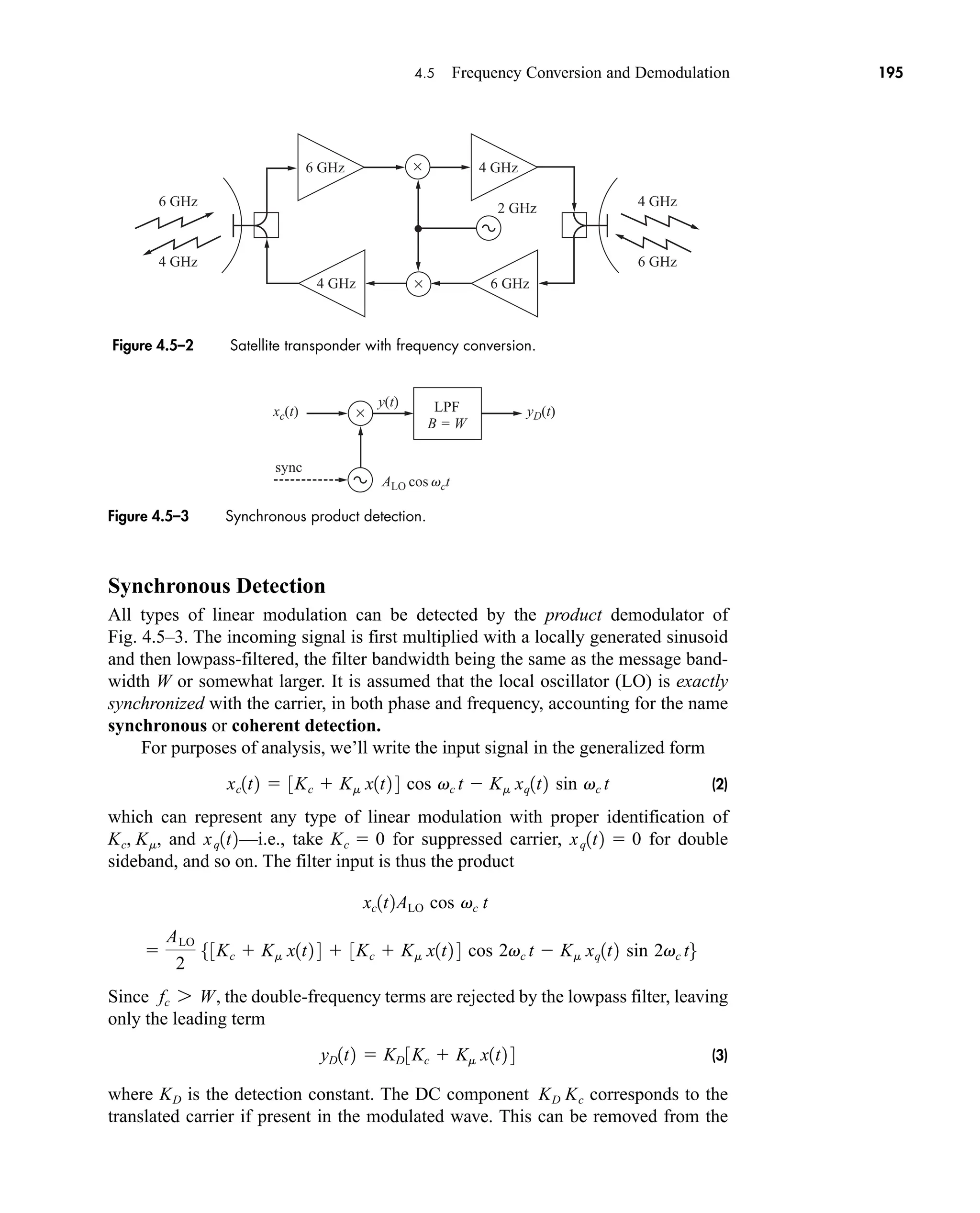
![fc + W
fc – W fc
a2d( f )
a1X( f )
a2[X( f ) * X( f )]
/2
1
a1d( f – fc)
a2X( f – fc)
/2
1
a2d( f – 2fc)
2fc
2W
0 W
/4
1
f
Figure 4.3–4 Spectral components in Eq. (1).
+
Ac cos vct
x(t)Ac cos vct
Ac [1 + x(t)] cos vct
x(t)
/2
1
/2
1
Ac [1 – x(t)] cos vct
/2
1
x(t)
/2
1
–
AM
mod
AM
mod
+
–
Figure 4.3–5 Balanced modulator.
+
–
xc(t)
x(t)
c(t)
vout
+
–
+
+–
–
BPF
Figure 4.3–6 Ring modulator.
4.3 Modulators and Transmitters 183
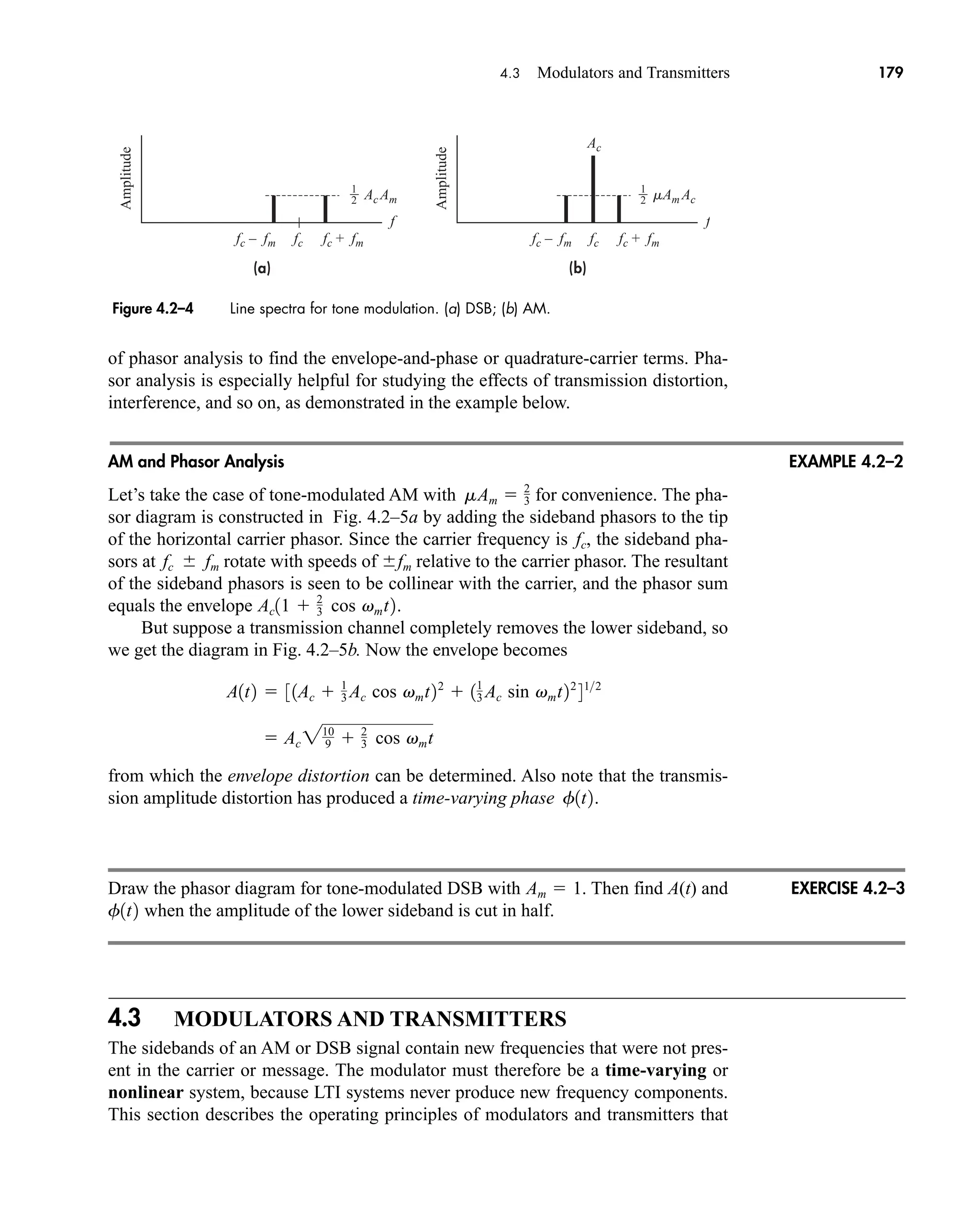
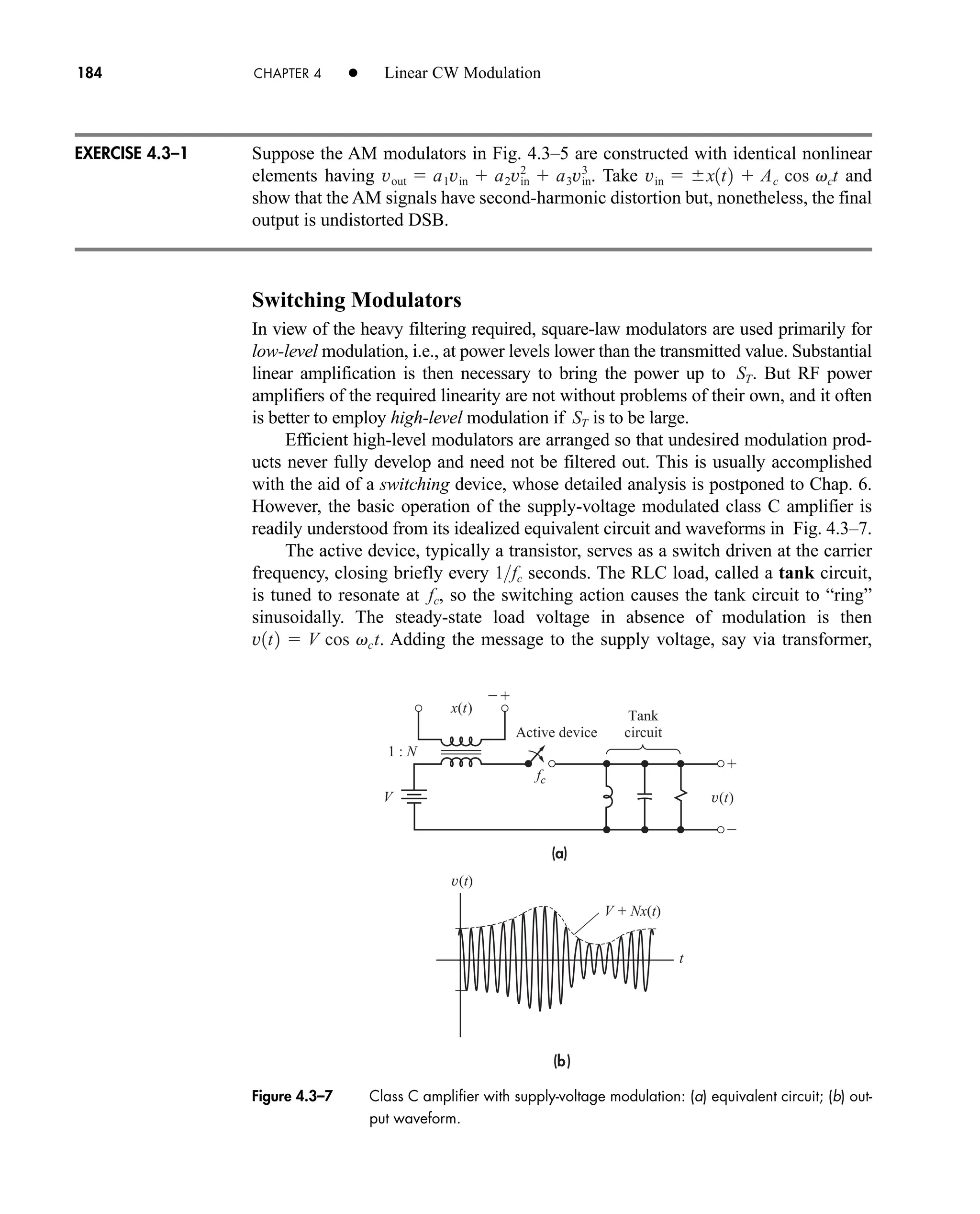
modulator can be thought of as multiplying x(t) and c(t). However because c(t) is a
periodic function, it can be represented by a Fourier series expansion. Thus
Observe that the DSB signal can be obtained by passing through a bandpass
filter having bandwidth 2W centered at . This modulator is often referred to as a
double-balanced modulator since it is balanced with respect to both x(t) and c(t).
A balanced modulator using switching circuits is discussed in Example 6.1–1
regarding bipolar choppers. Other circuit realizations can be found in the literature.
fc
vout1t2
vout1t2
4
p
x1t2 cos vct
4
3p
x1t2 cos 3vct
4
5p
x1t2 cos 5vct p
car80407_ch04_161-206.qxd 12/8/08 11:28 PM Page 183](https://image.slidesharecdn.com/communicationsystemsanintro-a-241115060943-61721fa8/75/Communication_Systems__An_Intro_-_A-_Bruce_Carlson_-pdf-205-2048.jpg)
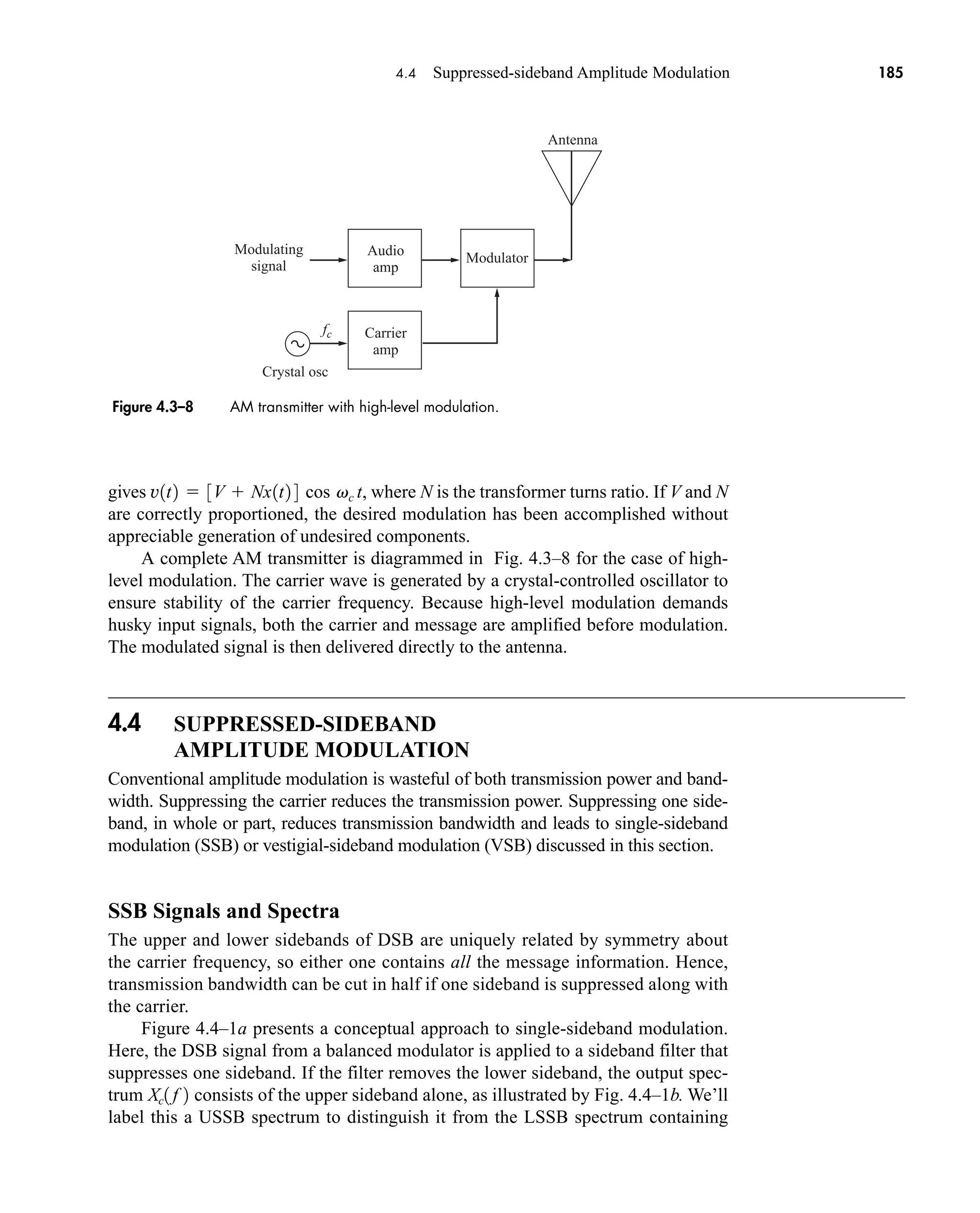
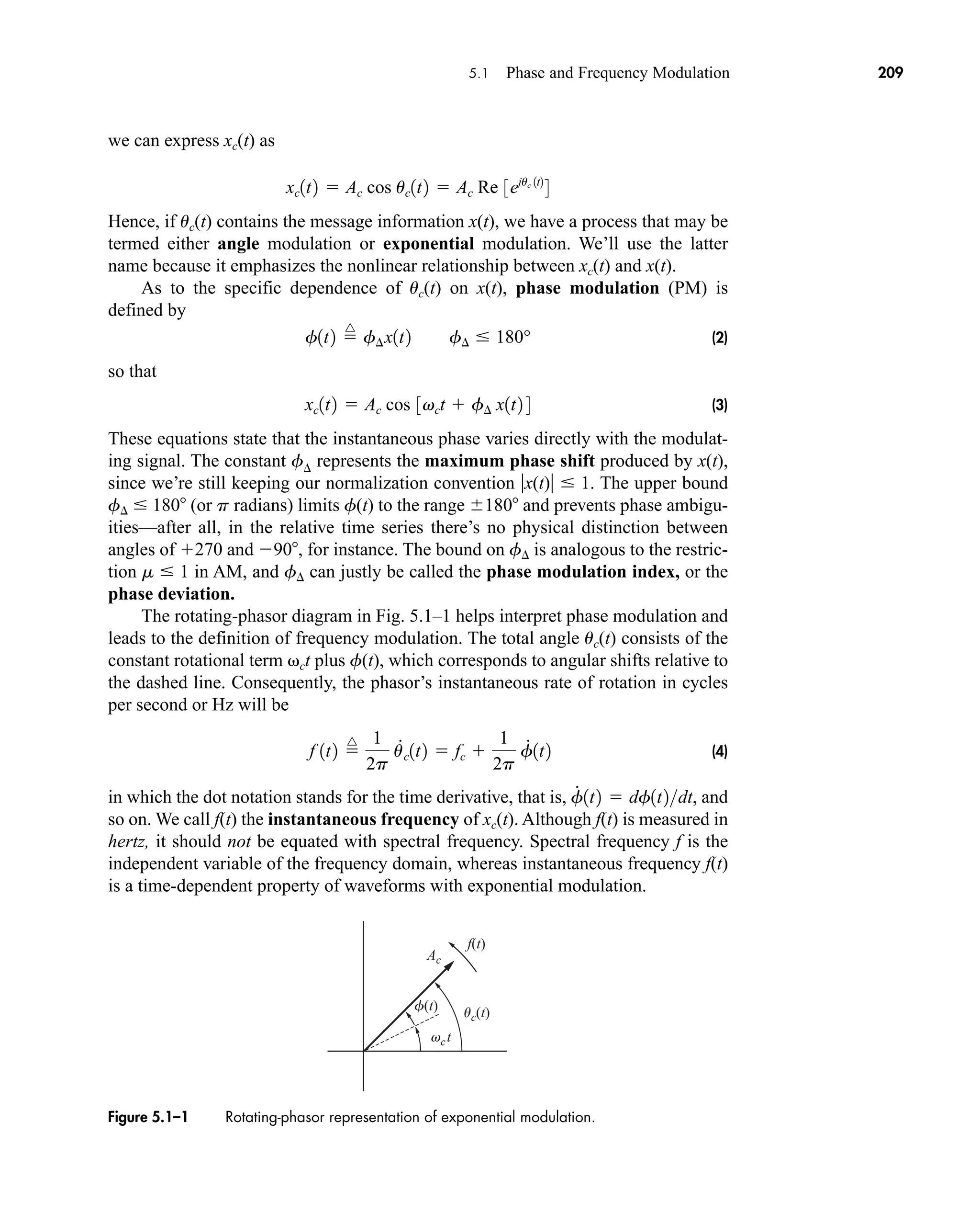
![AM
FM
PM
Modulating
signal
Figure 5.1–2 Illustrative AM, FM, and PM waveforms.
212 CHAPTER 5 • Angle CW Modulation
carrier amplitude, we modulate the frequency by swinging it over a range of, say,
50 Hz, then the transmission bandwidth will be 100 Hz regardless of the message
bandwidth. As we’ll soon see, this argument has a serious flaw, for it ignores the dis-
tinction between instantaneous and spectral frequency. Carson (1922) recognized
the fallacy of the bandwidth-reduction notion and cleared the air on that score.
Unfortunately, he and many others also felt that exponential modulation had no
advantages over linear modulation with respect to noise. It took some time to over-
come this belief but, thanks to Armstrong (1936), the merits of exponential modula-
tion were finally appreciated. Before we can understand them quantitatively, we
must address the problem of spectral analysis.
Suppose FM had been defined in direct analogy to AM by writing xc(t) Ac cos vc(t) t
with vc(t) vc[1 mx(t)]. Demonstrate the physical impossibility of this definition by
finding f(t) when x(t) cos vmt.
Narrowband PM and FM
Our spectral analysis of exponential modulation starts with the quadrature-carrier
version of Eq. (1), namely
(9)
where
(10)
xci1t2 Ac cos f1t2 Ac c1
1
2!
f2
1t2 p d
xc1t2 xci1t2 cos vct xcq1t2 sin vct
EXERCISE 5.1–1
car80407_ch05_207-256.qxd 12/8/08 10:49 PM Page 212](https://image.slidesharecdn.com/communicationsystemsanintro-a-241115060943-61721fa8/75/Communication_Systems__An_Intro_-_A-_Bruce_Carlson_-pdf-234-2048.jpg)
![(a) (b)
fc fc
Ac
2bfm
2bfm
Ac
b = 0.2
b = 1
b = 5
b = 10
5.1 Phase and Frequency Modulation 219
include the second-order pair of sideband lines that rotate at 2fm relative to the car-
rier and whose resultant is collinear with the carrier. While the second-order pair vir-
tually wipes out the undesired amplitude modulation, it also distorts f(t). The phase
distortion is then corrected by adding the third-order pair, which again introduces
amplitude modulation, and so on ad infinitum.
When all spectral lines are included, the odd-order pairs have a resultant in
quadrature with the carrier that provides the desired frequency modulation plus
unwanted amplitude modulation. The resultant of the even-order pairs, being
collinear with the carrier, corrects for the amplitude variations. The net effect is then
as illustrated in Fig. 5.1–8. The tip of the resultant sweeps through a circular arc
reflecting the constant amplitude Ac.
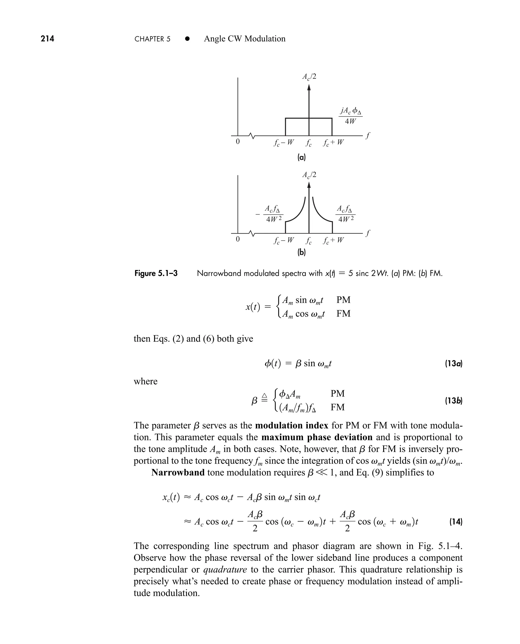
Tone Modulation With NBFM
The narrowband FM signal xc(t) 100 cos [2p 5000t 0.05 sin 2p 200t] is trans-
mitted. To find the instantaneous frequency f(t) we take the derivative of u(t)
5000 10 cos 2p 200 t
1
2p
32p 5000 0.0512p 2002 cos 2p 200 t4
f1t2
1
2p
u
#
1t2
Figure 5.1–7 Single-tone-modulated line spectra: (a) FM or PM with fm fixed; (b) FM with
Amf fixed.
EXAMPLE 5.1–2
car80407_ch05_207-256.qxd 12/8/08 10:49 PM Page 219](https://image.slidesharecdn.com/communicationsystemsanintro-a-241115060943-61721fa8/75/Communication_Systems__An_Intro_-_A-_Bruce_Carlson_-pdf-241-2048.jpg)
![EXERCISE 5.1–3
Ac
Even-order
sidebands
Odd-order
sidebands
Figure 5.1–8 FM phasor diagram for arbitrary b.
220 CHAPTER 5 • Angle CW Modulation
From f(t) we determine that fc 5000 Hz, f 10, and x(t) cos 2p 200t. There
are two ways to find b. For NBFM with tone modulation we know that
f(t) b sin vmt. Since xc(t) Ac cos [vct f(t)], we can see that b 0.05. Alter-
natively we can calculate
From f(t) we find that Amf 10 and fm 200 so that b 10/200 0.05 just as
we found earlier. The line spectrum has the form of Fig. 5.1–4a with Ac 100 and
sidelobes Acb /2 2.5. The minor distortion from the narrowband approximation shows
up in the transmitted power. From the line spectrum we get
versus when there are
enough sidelobes so that there is no amplitude distortion.
Consider tone-modulated FM with Ac 100, Am f 8 kHz, and fm 4 kHz. Draw
the line spectrum for fc 30 kHz and for fc 11kHz.
Multitone and Periodic Modulation
The Fourier series technique used to arrive at Eq. (18) also can be applied to the case
of FM with multitone modulation. For instance, suppose that x(t) A1 cos v1t
A2 cos v2t, where f1 and f2 are not harmonically related. The modulated wave is first
written as
xc1t2 Ac 31cos a1 cos a2 sin a1 sin a2 2 cos vct
ST 1
2 Ac
2
1
2110022
5000
1
2 110022
1
2 12.522
5006.25
ST 1
2 12.522
b
Am
fm
f¢
car80407_ch05_207-256.qxd 12/15/08 10:04 PM Page 220](https://image.slidesharecdn.com/communicationsystemsanintro-a-241115060943-61721fa8/75/Communication_Systems__An_Intro_-_A-_Bruce_Carlson_-pdf-242-2048.jpg)
![5.2 Transmission Bandwidth and Distortion 229
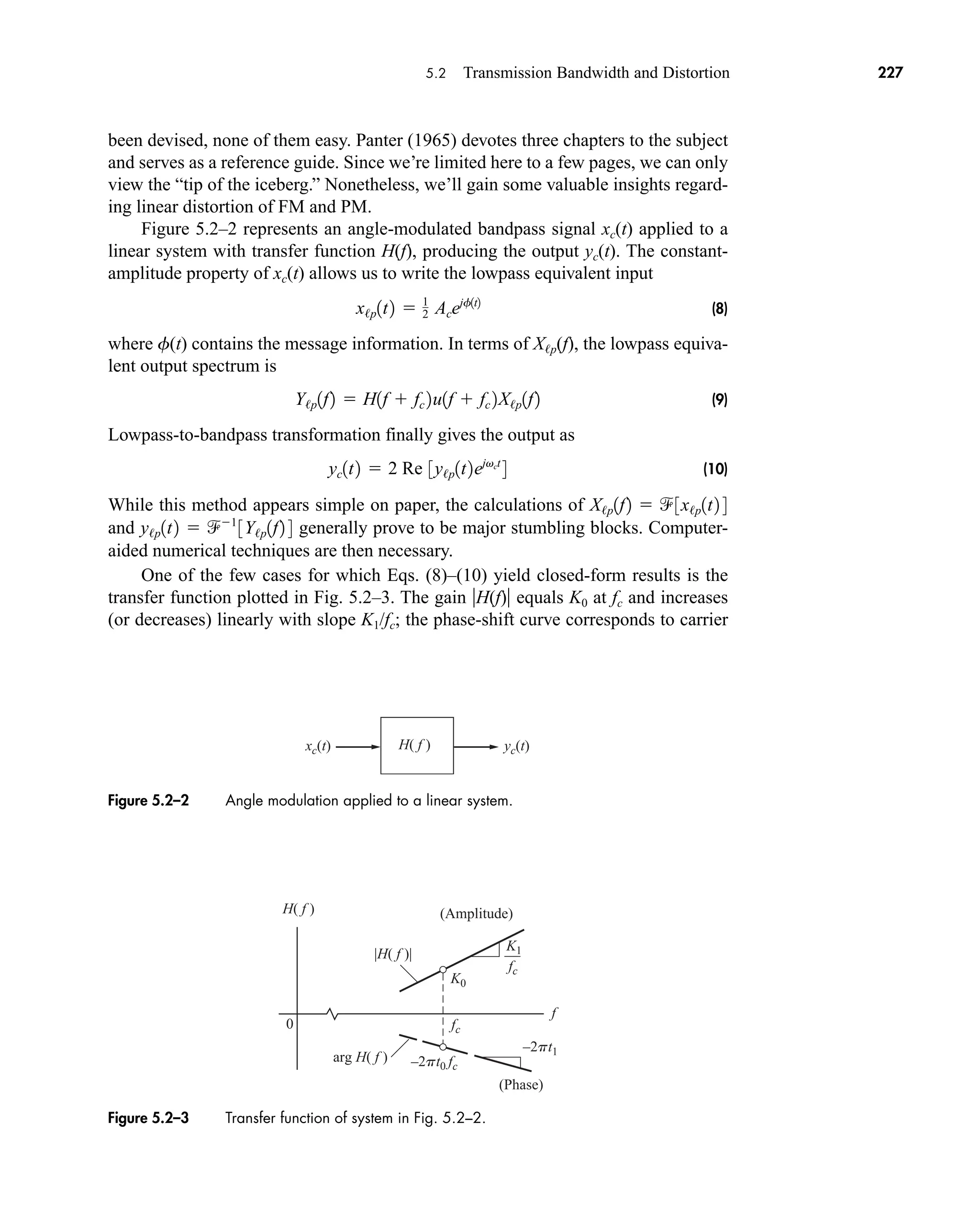
ordinary sinusoid at frequency f(t) fc f x(t). For if the system’s response to a
carrier-frequency sinusoid is
and if xc(t) has a slowly changing instantaneous frequency f(t), then
(13)
It can be shown that this approximation requires the condition
(14)
in which for tone-modulated FM with fm W. If H(f) represents a
single-tuned bandpass filter with 3 dB bandwidth B, then the second term in Eq. (14)
equals 8/B2
and the condition becomes 4fW/B2
V 1 which is satisfied by the trans-
mission bandwidth requirement B BT.
Now suppose that Eq. (14) holds and the system has a nonlinear phase shift such
as arg H( f) af 2
, where a is a constant. Upon substituting
we get
Thus, the total phase in Eq. (13) will be distorted by the addition of and
Let H(f) 1 and arg H(f) 2pt1(f fc). Show that Eqs. (11) and (13) give the
same result with f(t) b sin vmt provided that vmt1 V p.
Nonlinear Distortion and Limiters
Amplitude distortion of an FM wave produces FM-to-AM conversion. Here we’ll
show that the resulting AM can be eliminated through the use of controlled
nonlinear distortion and filtering.
For purposes of analysis, let the input signal in Fig. 5.2–4 be
where uc(t) vct f(t) and A(t) is the amplitude. The nonlinear element is assumed
to be memoryless—meaning no energy storage—so the input and output are related
by an instantaneous nonlinear transfer characteristic vout T[vin]. We’ll also assume
for convenience that T[0] 0.
Although vin(t) is not necessarily periodic in time, it may be viewed as a
periodic function of uc with period 2p. (Try to visualize plotting vin versus uc with
vin1t2 A1t2 cos uc1t2
f
# 2
1t2.
f
#
1t2
arg H 3 f 1t2 4 a f c
2
a fc
p
f
#
1t2
a
4p2 f
#2
1t2
f1t2 fc f
#
1t22p
0 f
.
.
1t2 0 4p2
f¢W
0f
..
1t20max `
1
H1 f 2
d2
H1 f 2
df 2 `
max
V 8p2
yc1t2 AcH3f 1t2 4 cos 5vct f1t2 arg H3f 1t2 46
yc1t2 AcH1fc 2 cos 3vct arg H1fc 2 4
EXERCISE 5.2–2
car80407_ch05_207-256.qxd 1/13/09 4:03 PM Page 229
Rev.Confirming Pages](https://image.slidesharecdn.com/communicationsystemsanintro-a-241115060943-61721fa8/75/Communication_Systems__An_Intro_-_A-_Bruce_Carlson_-pdf-251-2048.jpg)
![vin(t) vout(t) = T [vin(t)]
Nonlinear element
Figure 5.2–4 Nonlinear system to reduce envelope variations (AM).
230 CHAPTER 5 • Angle CW Modulation
time held fixed.) Likewise, the output is a periodic function of uc and can be
expanded in the trigonometric Fourier series
(15a)
where
(15b)
The time variable t does not appear explicitly here, but vout depends on t via the time-
variation of uc. Additionally, the coefficients an may be functions of time when the
amplitude of vin has time variations.
But we’ll first consider the case of an undistorted FM input, so A(t) equals the
constant Ac and all the an are constants. Hence, writing out Eq. (15a) term by term
with t explicitly included, we have
(16)
This expression reveals that the nonlinear distortion produces additional FM waves
at harmonics of the carrier frequency, the nth harmonic having constant amplitude
2an and phase modulation nf(t) plus a constant phase shift arg an.
If these waves don’t overlap in the frequency domain, the undistorted input
can be recovered by applying the distorted output to a bandpass filter. Thus, we
say that FM enjoys considerable immunity from the effects of memoryless nonlin-
ear distortion.
Now let’s return to FM with unwanted amplitude variations A(t). Those varia-
tions can be flattened out by an ideal hard limiter or clipper whose transfer char-
acteristic is plotted in Fig. 5.2–5a. Figure 5.2–5b shows a clipper circuit that uses a
comparator or high-gain operational amplifier such that any input voltages greater
or less than zero cause the output to reach either the positive or negative power sup-
ply rails.
The clipper output looks essentially like a square wave, since T[vin] V0 sgn vin
and
vout e
V0 vin 7 0
V0 vin 6 0
p
02a2 0 cos 32vc t 2f1t2 arg a2 4
vout1t2 02a1 0 cos 3vc t f1t2 arg a1 4
an
1
2p 2p
T 3vin 4ejnuc
duc
vout a 0
q
n1
2an 0 cos 1n uc arg an 2
car80407_ch05_207-256.qxd 12/15/08 10:04 PM Page 230](https://image.slidesharecdn.com/communicationsystemsanintro-a-241115060943-61721fa8/75/Communication_Systems__An_Intro_-_A-_Bruce_Carlson_-pdf-252-2048.jpg)
![(a)
(b)
A(t) cos [vct + f(t)]
Ac cos [vct + f(t)]
cos [vct + f(t)]
|2an| cos [nvct + nf(t) + arg an]
4V0
BPF
at fc
BPF
at n fc
p
(a) (b)
vin
vin
vout
vin
+ V0 + +
+
−
−
−
– V0
0
Figure 5.2–5 Hard limiter: (a) transfer characteristic; (b) circuit realization with Zener diodes.
5.2 Transmission Bandwidth and Distortion 231
Figure 5.2–6 Nonlinear processing circuits: (a) amplitude limiter; (b) frequency multiplier.
The coefficients are then found from Eq. (15b) to be
which are independent of time because the amplitude A(t) 0 does not affect the
sign of vin. Therefore,
(17)
and bandpass filtering yields a constant-amplitude FM wave if the components of
vout(t) have no spectral overlap. Incidentally, this analysis lends support to the previ-
ous statement that the message information resides entirely in the zero-crossings of
an FM or PM wave.
Figure 5.2–6 summarizes our results. The limiter plus BPF in part a removes
unwanted amplitude variations from an AM or PM wave, and would be used in a
receiver. The nonlinear element in part b distorts a constant-amplitude wave, but the
BPF passes only the undistorted term at the nth harmonic. This combination acts as
a frequency multiplier if n 1, and is used in certain types of transmitters.
vout1t2
4V0
p
cos3vct f1t2 4
4V0
3p
cos 33vct 3f1t2 4 p
an •
2V0pn n 1, 5, 9, p
2V0pn n 3, 7, 11, p
0 n 2, 4, 6, p
car80407_ch05_207-256.qxd 1/19/09 10:15 AM Page 231
Rev.Confirming Pages](https://image.slidesharecdn.com/communicationsystemsanintro-a-241115060943-61721fa8/75/Communication_Systems__An_Intro_-_A-_Bruce_Carlson_-pdf-253-2048.jpg)

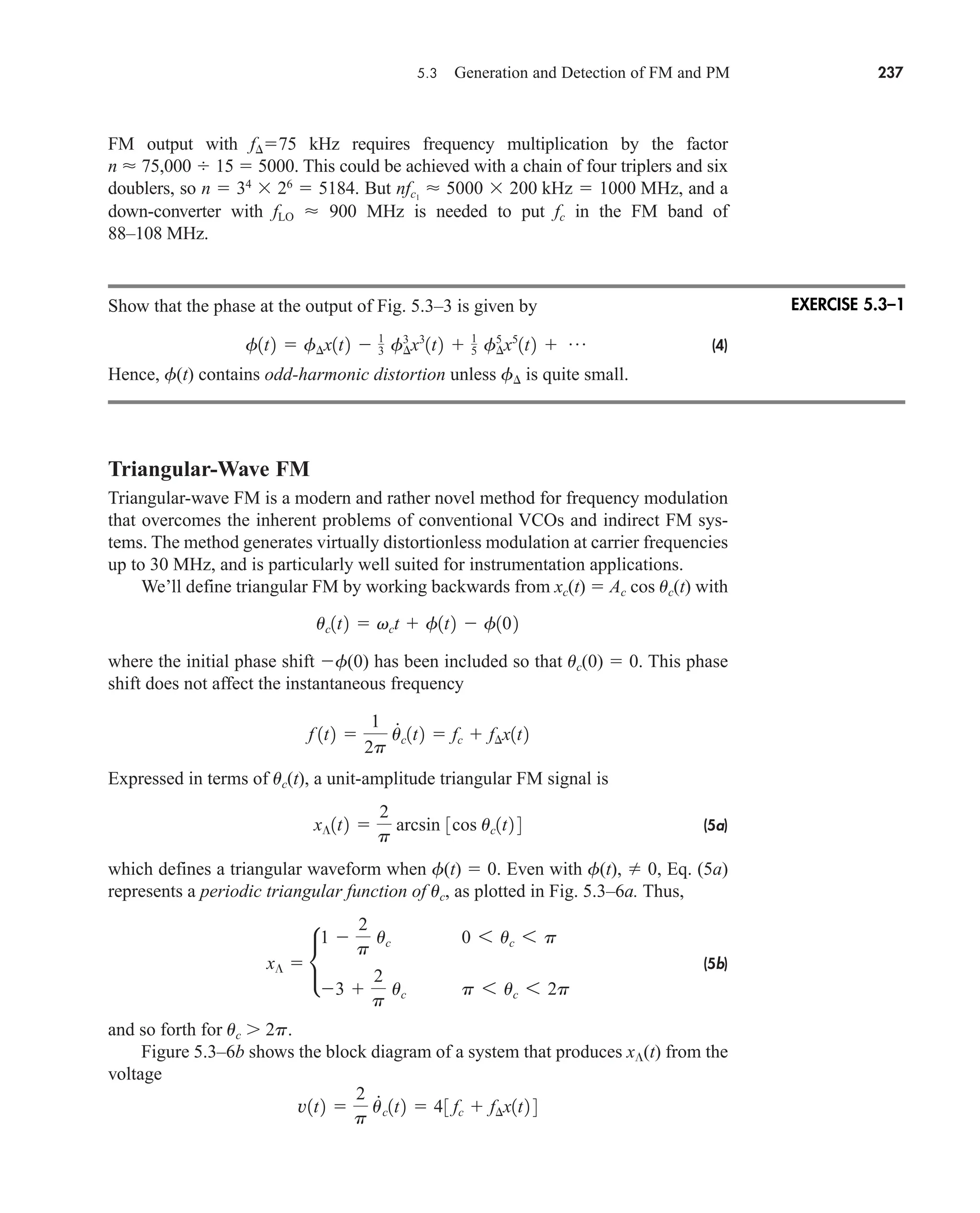
![(b)
(a)
xΛ(t)
v(t) = 2 uc(t)
= 4[ fc + f∆x(t)]
∫
uc
xΛ
1
0
Schmitt trigger
Electronic switch
–1
–1
–2
p 3p/2
–p/2 2p
•
p
238 CHAPTER 5 • Angle CW Modulation
which is readily derived from the message waveform x(t). The system consists of an
analog inverter, an integrator, and a Schmitt trigger controlling an electronic switch.
The trigger puts the switch in the upper position whenever x(t) increases to 1 and
puts the switch in the lower position whenever x(t) decreases to 1.
Suppose the system starts operating at t 0 with x(0) 1 and the switch in
the upper position. Then, for 0 t t1,
so x(t) traces out the downward ramp in Fig. 5.3–6a until time t1 when x(t1) 1,
corresponding to uc(t1) p. Now the trigger throws the switch to the lower position
and
so x(t) traces out the upward ramp in Fig. 5.3–6a. The upward ramp continues until
time t2 when uc(t2) 2p and x(t2) 1. The switch then triggers back to the upper
position, and the operating cycle goes on periodically for t t2.
3
2
p
uc1t2 t1 6 t 6 t2
x¶1t2 1
t
t1
v1l2 dl 1
2
p
3uc1t2 uc1t1 2 4
1
2
p
uc1t2 0 6 t 6 t1
x¶1t2 1
t
0
v1l2 dl 1
2
p
3uc1t2 uc102 4
Figure 5.3–6 Triangular-wave FM: (a) waveform; (b) modulation system.
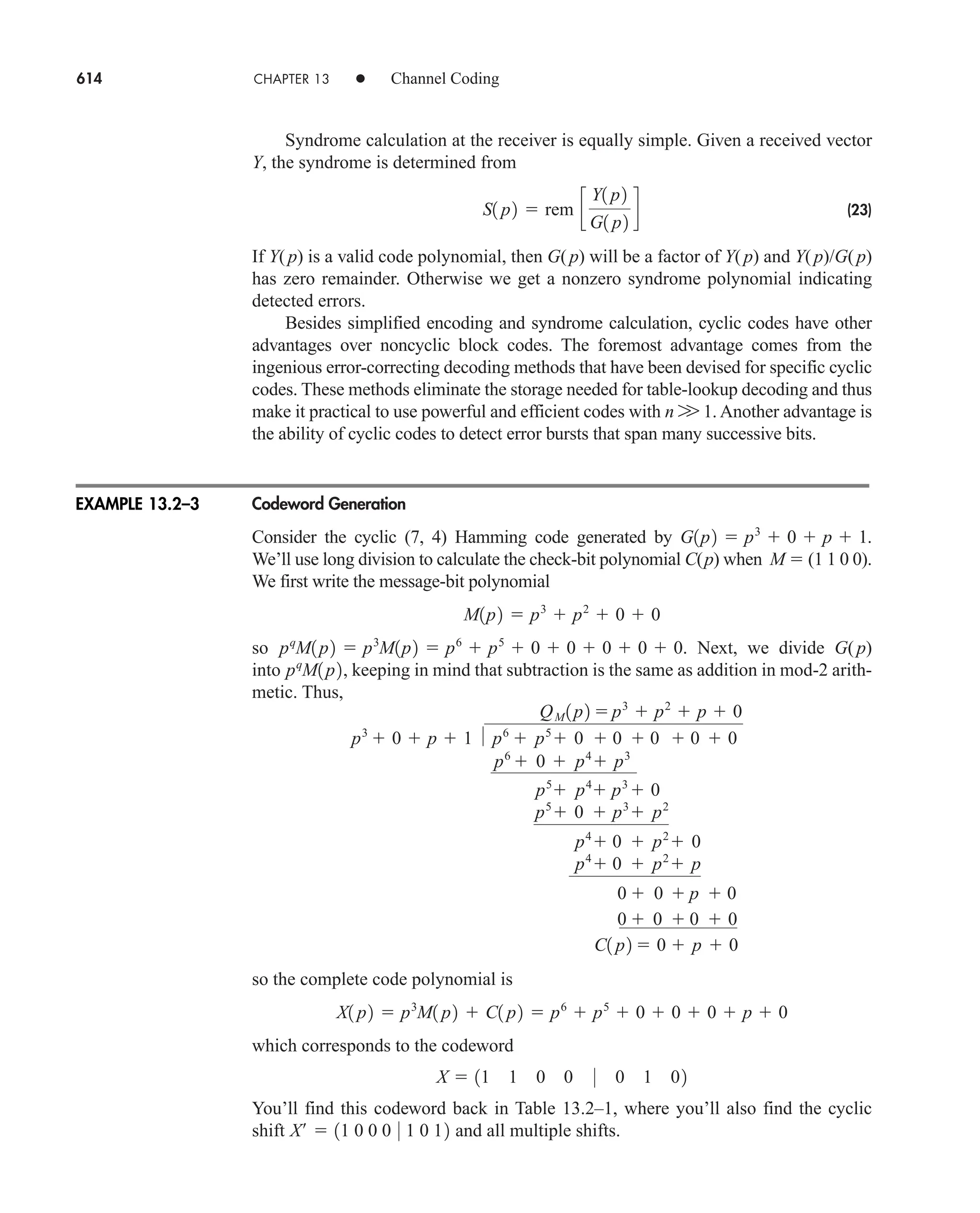
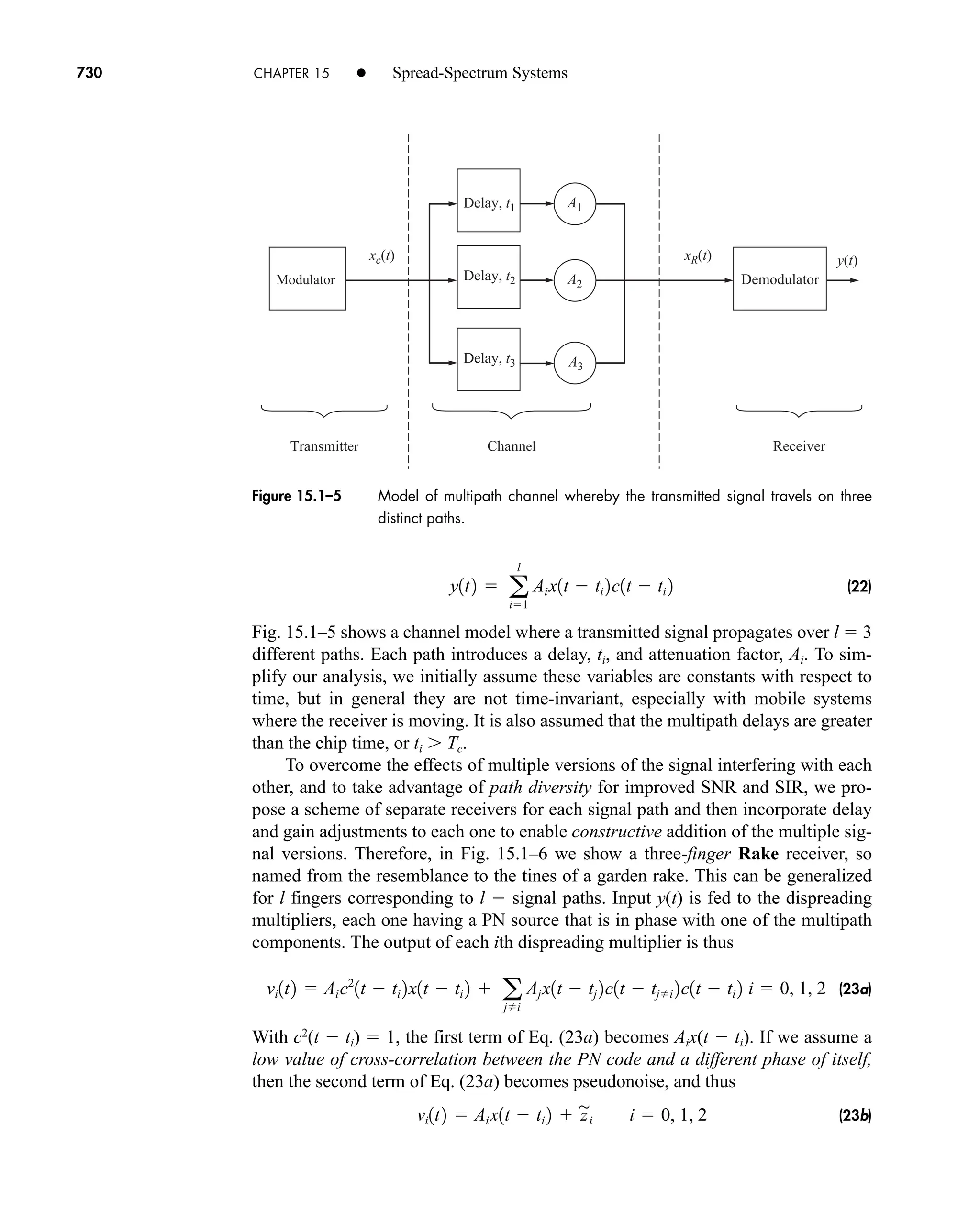
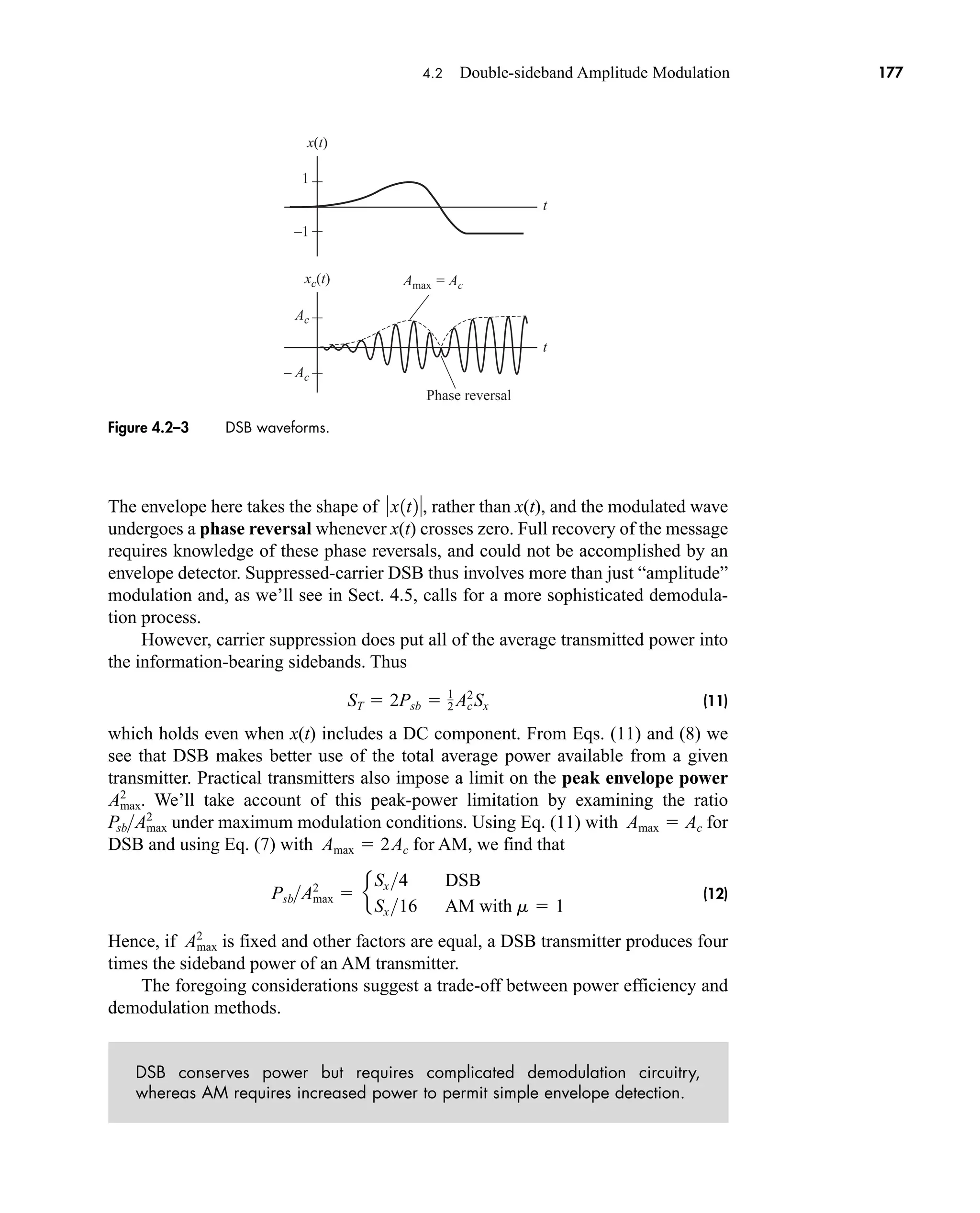
car80407_ch05_207-256.qxd 12/8/08 10:49 PM Page 238](https://image.slidesharecdn.com/communicationsystemsanintro-a-241115060943-61721fa8/75/Communication_Systems__An_Intro_-_A-_Bruce_Carlson_-pdf-260-2048.jpg)
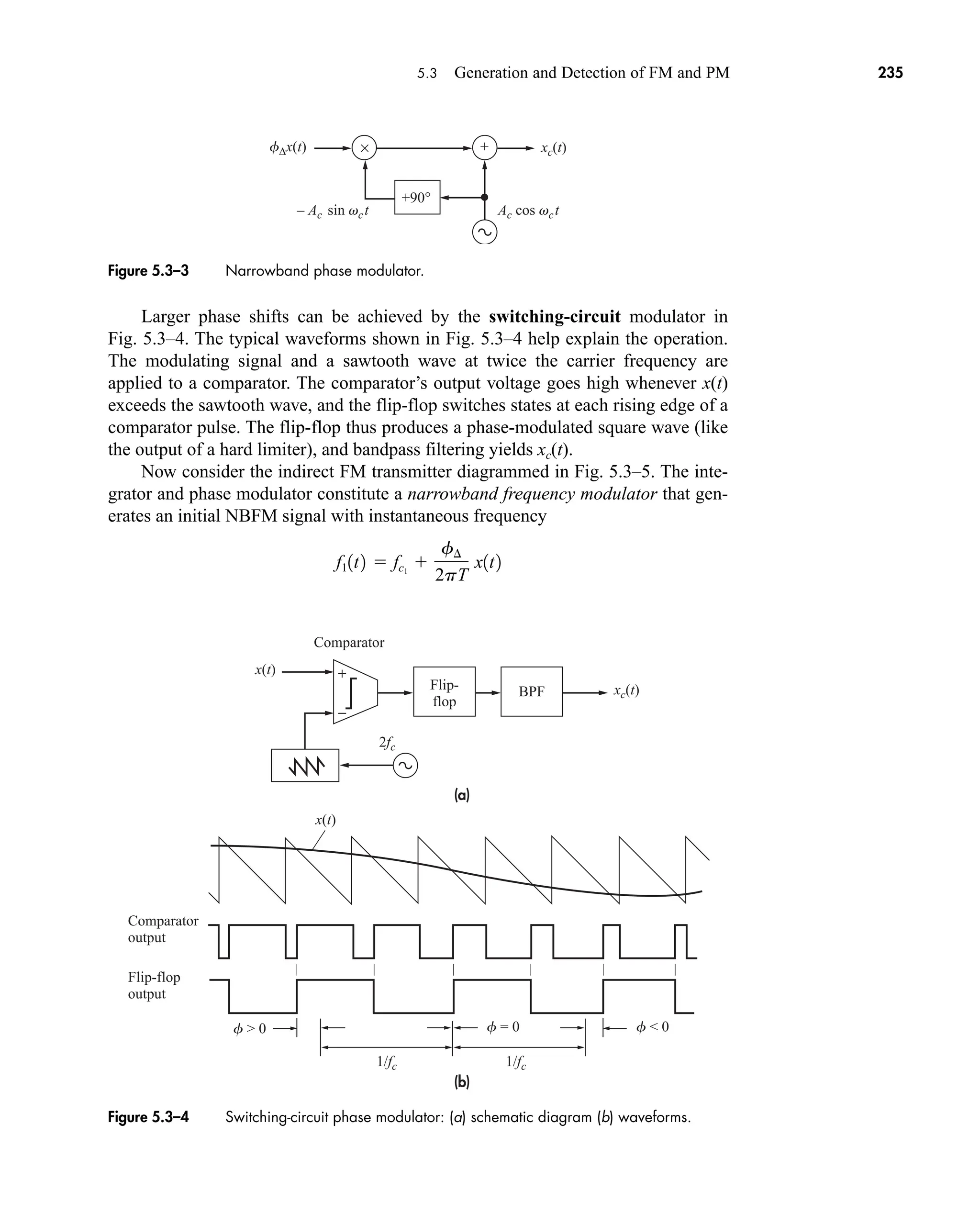
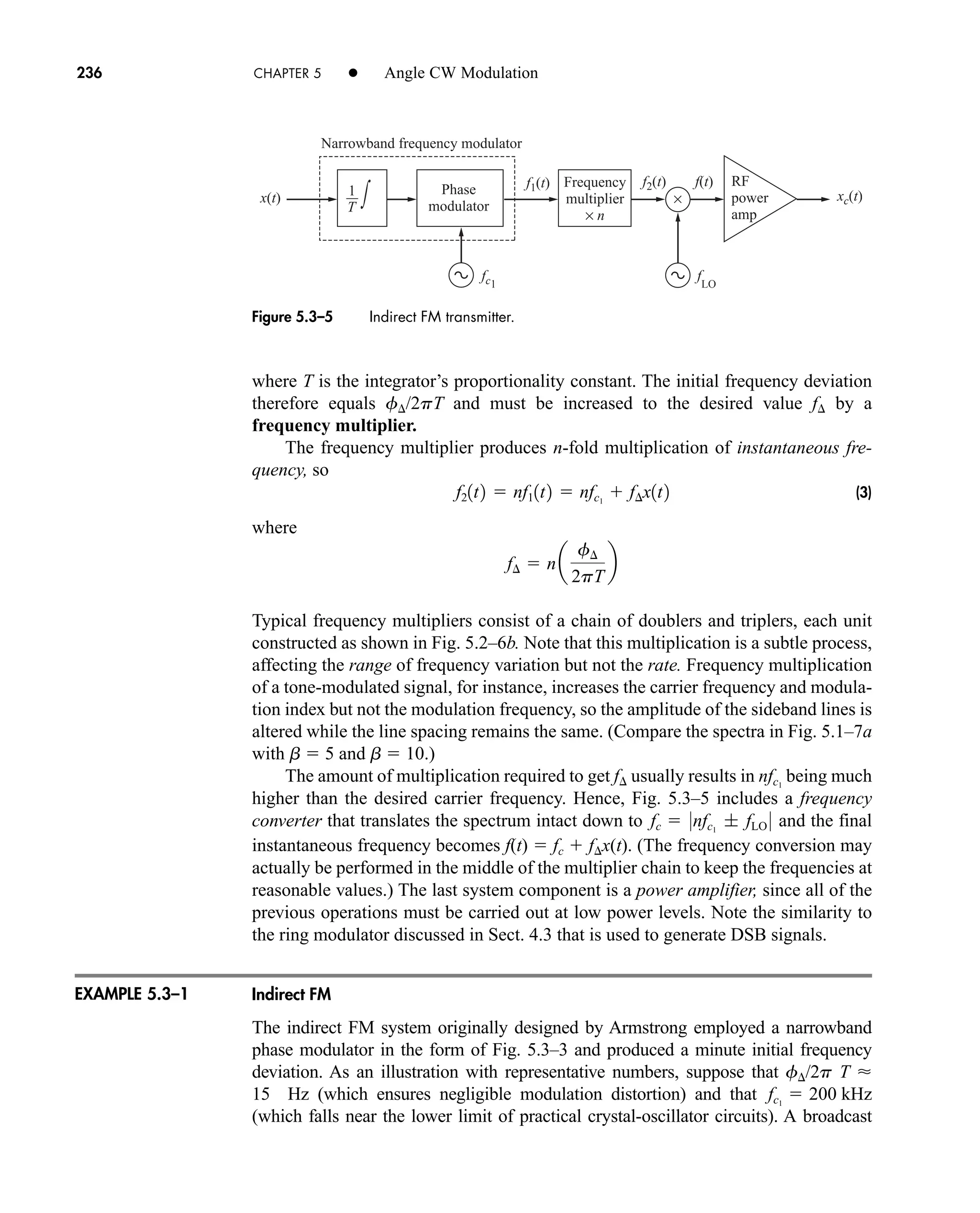
![5.3 Generation and Detection of FM and PM 239
A sinusoidal FM wave is obtained from x(t) using a nonlinear waveshaper with
transfer characteristics T[x(t)] Ac sin [(p/2)x(t)], which performs the inverse of
Eq. (5a). Or x(t) can be applied to a hard limiter to produce square-wave FM. A
laboratory test generator might have all three outputs available.
Frequency Detection
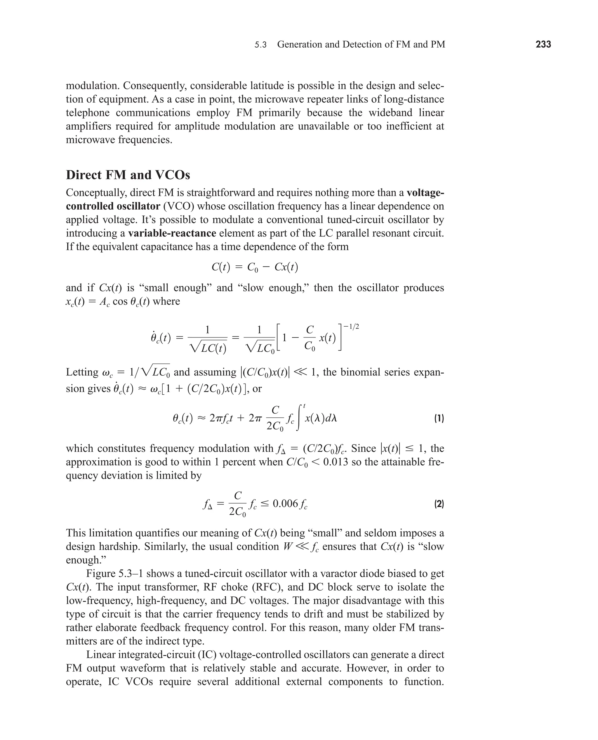
A frequency detector, often called a discriminator, produces an output voltage that
should vary linearly with the instantaneous frequency of the input. There are perhaps
as many different circuit designs for frequency detection as there are designers who
have considered the problem. However, almost every circuit falls into one of the fol-
lowing four operational categories:
1. FM-to-AM conversion
2. Phase-shift discrimination
3. Zero-crossing detection
4. Frequency feedback
We’ll look at illustrative examples from the first three categories, postponing fre-
quency feedback to Sect. 7.3. Analog phase detection is not discussed here because
it’s seldom needed in practice and, if needed, can be accomplished by integrating the
output of a frequency detector.
Any device or circuit whose output equals the time derivative of the input pro-
duces FM-to-AM conversion. To be more specific, let xc(t) Ac cos uc(t) with
then
(6)
Hence, an envelope detector with input yields an output proportional to
f(t) fc fx(t).
Figure 5.3–7a diagrams a conceptual frequency detector based on Eq. (6). The dia-
gram includes a limiter at the input to remove any spurious amplitude variations from
xc(t) before they reach the envelope detector. It also includes a DC block to remove the
constant carrier-frequency offset from the output signal. Typical waveforms are
sketched in Fig. 5.3–7b taking the case of tone modulation. A LPF has been included
after the limiter to remove waveform discontinuities and thereby facilitate differentia-
tion. However with slope detection, filtering and differentiation occur in the same stage.
For actual hardware implementation of FM-to-AM conversion, we draw upon the
fact that an ideal differentiator has . Slightly above or below resonance,
the transfer function of an ordinary tuned circuit shown in Fig. 5.3–8a approximates
the desired linear amplitude response over a small frequency range. Thus, for
instance, a detuned AM receiver will roughly demodulate FM via slope detection.
Extended linearity is achieved by the balanced discriminator circuit in
Fig. 5.3–8b. A balanced discriminator includes two resonant circuits, one tuned
above fc and the other below, and the output equals the difference of the two
0H1 f 2 0 2pf
x
#
c1t2
2pAc 3fc f¢ x1t2 4 sin 3uc1t2 ; 180°4
.
xc1t2 Acu
.
c1t2 sin uc1t2
u
#
c1t2 2p3fc f¢x1t2 4;
car80407_ch05_207-256.qxd 12/15/08 10:04 PM Page 239](https://image.slidesharecdn.com/communicationsystemsanintro-a-241115060943-61721fa8/75/Communication_Systems__An_Intro_-_A-_Bruce_Carlson_-pdf-261-2048.jpg)
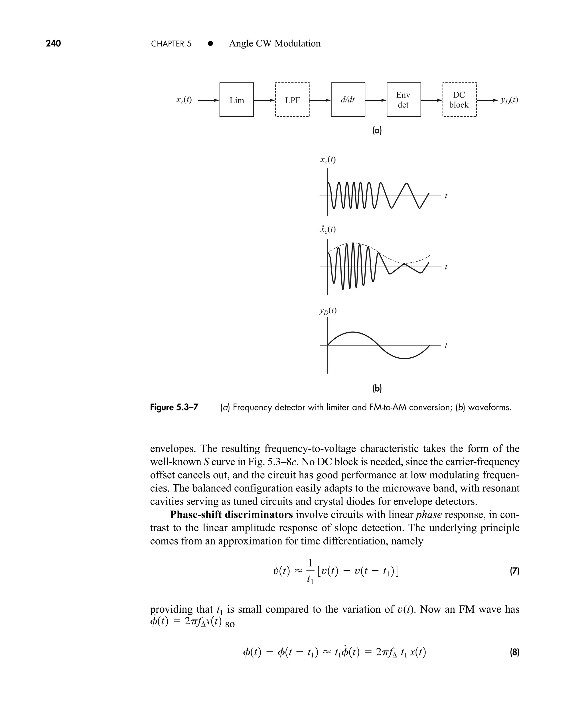
![(a)
(b)
(c)
Kx(t)
xc(t)
fc
fc
f0
f0 fc
f0 fc
f
f
Slope
approximation
|H( f )|
+
–
+
–
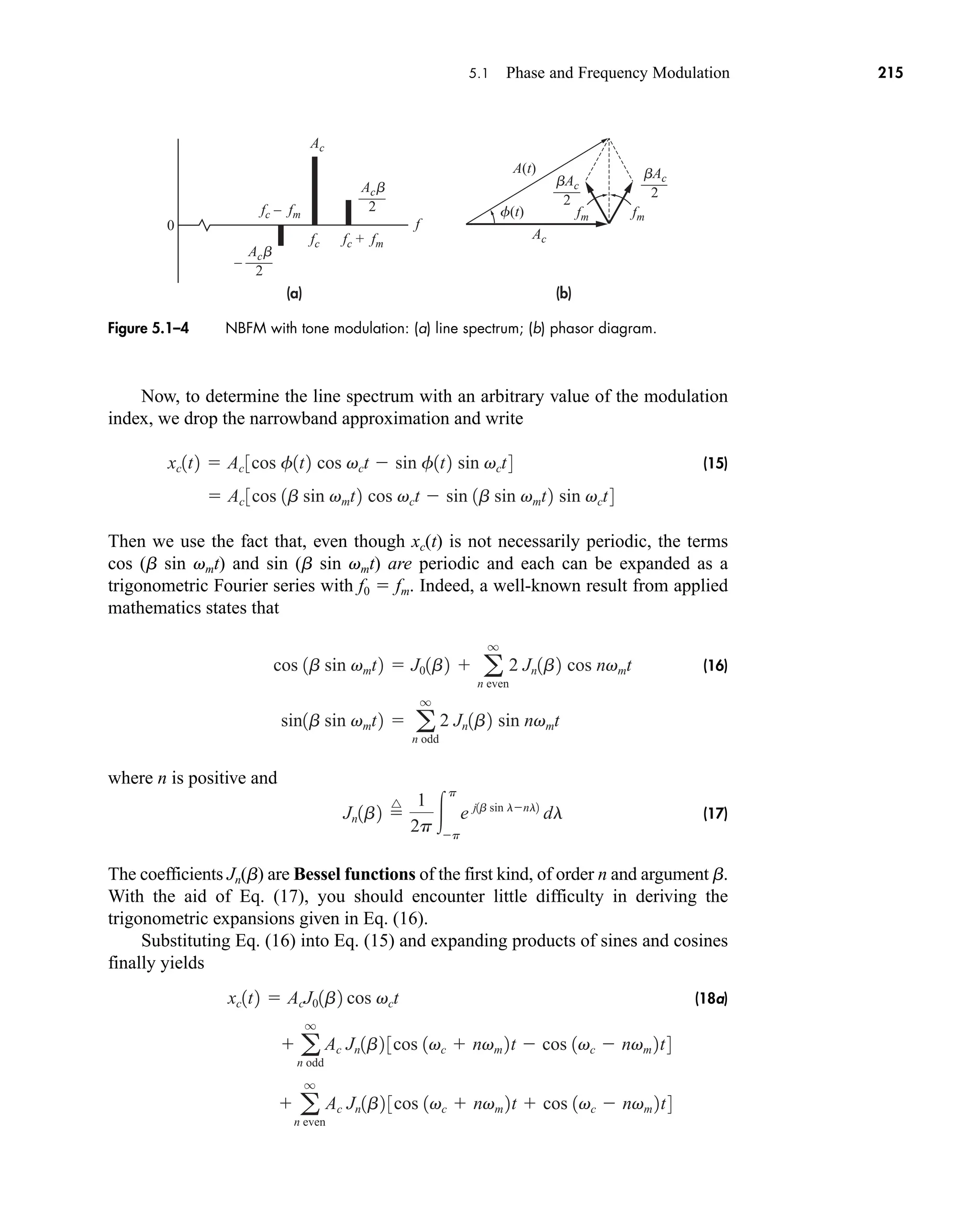
5.3 Generation and Detection of FM and PM 241
The term f(t t1) can be obtained with the help of a delay line or, equivalently, a
linear phase-shift network.
Figure 5.3–9 represents a phase-shift discriminator built with a network having
group delay t1 and carrier delay t0 such that vct0 90—which accounts for the
name quadrature detector. From Eq. (11), Sect. 5.2, the phase-shifted signal is pro-
portional to cos[vct 90 f(t t1)] sin [vct f(t t1)]. Multiplication by
cos [vct f(t)] followed by lowpass filtering yields an output proportional to
sin3f1t2 f1t t1 2 4 f1t2 f1t t1 2
Figure 5.3–8 (a) Slope detection with a tuned circuit; (b) balanced discriminator circuit;
(c) frequency-to-voltage characteristic.
car80407_ch05_207-256.qxd 12/8/08 10:49 PM Page 241](https://image.slidesharecdn.com/communicationsystemsanintro-a-241115060943-61721fa8/75/Communication_Systems__An_Intro_-_A-_Bruce_Carlson_-pdf-263-2048.jpg)
![cos [vct + f(t)]
sin [vct + f(t – t1)]
xc(t) ×
Lim BPF LPF
Phase-shift
network
y
D(t) KD f∆x(t)
242 CHAPTER 5 • Angle CW Modulation
assuming t1 is small enough that f(t) f(t t1)V p. Therefore,
where the detection constant KD includes t1. Despite these approximations, a quadra-
ture detector provides better linearity than a balanced discriminator and is often
found in high-quality receivers.
Other phase-shift circuit realizations include the Foster-Seely discriminator
and the popular ratio detector. The latter is particularly ingenious and economical,
for it combines the operations of limiting and demodulation into one unit. See
Tomasi (1998, Chap. 7) for further details.
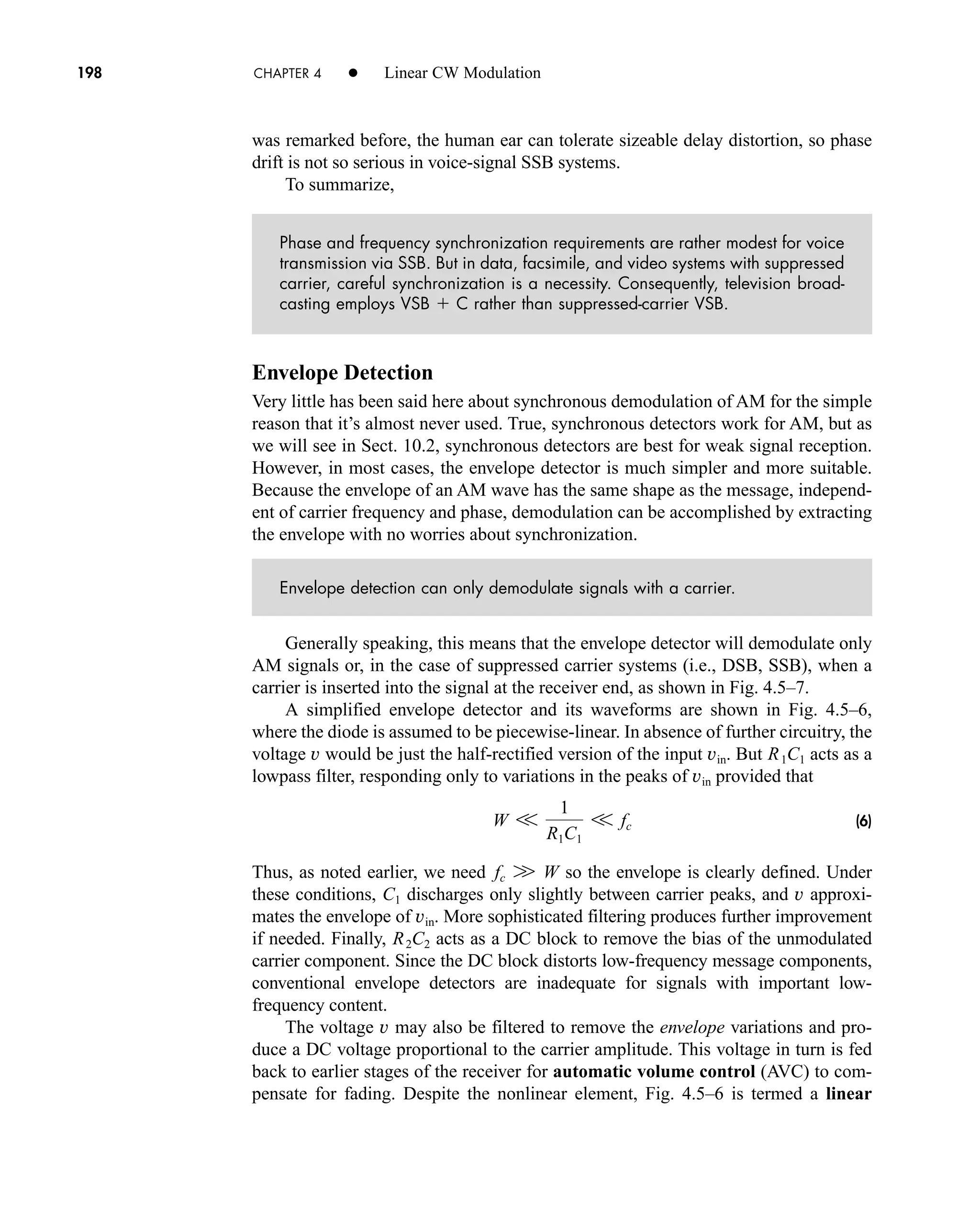
Lastly, Fig. 5.3–10 gives the diagram and waveforms for a simplified zero-
crossing detector. The square-wave FM signal from a hard limiter triggers a
monostable pulse generator, which produces a short pulse of fixed amplitude A and
duration t at each upward (or downward) zero crossing of the FM wave. If we invoke
the quasi-static viewpoint and consider a time interval T such that W V 1/T V fc,
the monostable output v(t) looks like a rectangular pulse train with nearly constant
period 1/f(t). Thus, there are nT Tf(t) pulses in this interval, and continually inte-
grating v(t) over the past T seconds yields
which becomes yD(t) KD fx(t) after the DC block.
Commercial zero-crossing detectors may have better than 0.1 percent linearity
and operate at center frequencies from 1 Hz to 10 MHz. A divide-by-ten counter
inserted after the hard limiter extends the range up to 100 MHz.
Today most FM communication devices utilize linear integrated circuits for FM
detection. Their reliability, small size, and ease of design have fueled the growth of
portable two-way FM and cellular radio communications systems. Phase-locked
loops and FM detection will be discussed in Sect. 7.3.
Given a delay line with time delay t0 V 1/fc, devise a frequency detector based on
Eqs. (6) and (7).
1
T
t
tT
v1l2 dl
1
T
nT At Atf 1t2
yD1t2 KDf¢x1t2
Figure 5.3–9 Phase-shift discriminator or quadrature detector.
EXERCISE 5.3–2
car80407_ch05_207-256.qxd 12/8/08 10:49 PM Page 242](https://image.slidesharecdn.com/communicationsystemsanintro-a-241115060943-61721fa8/75/Communication_Systems__An_Intro_-_A-_Bruce_Carlson_-pdf-264-2048.jpg)
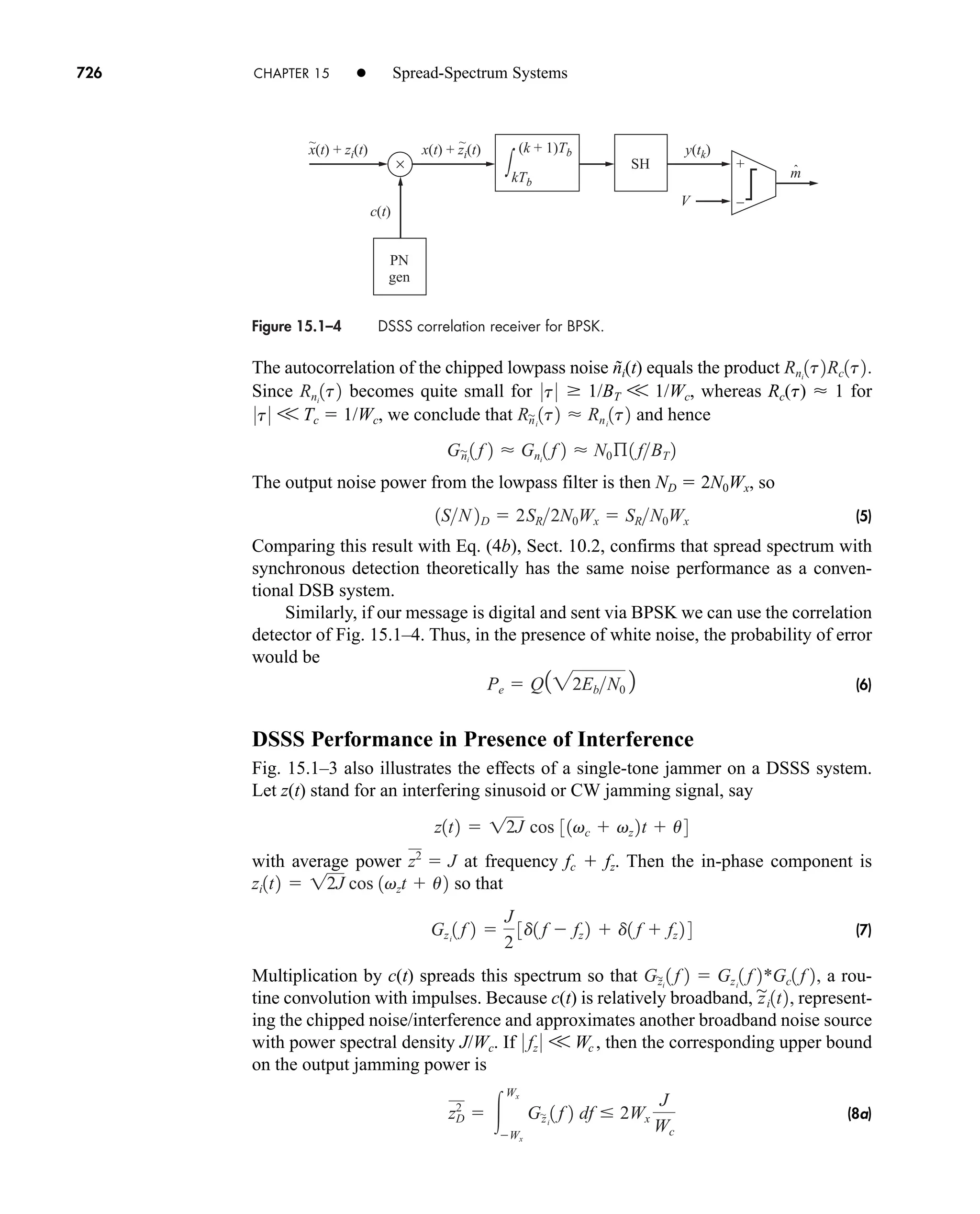
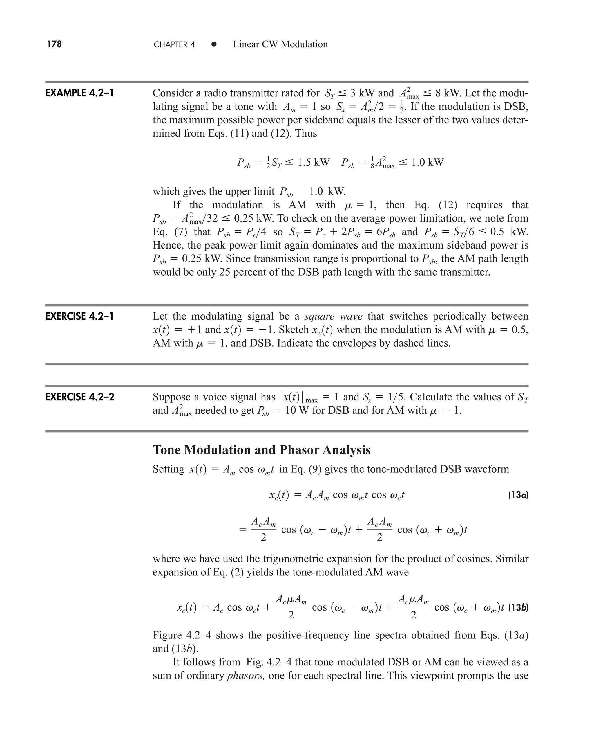
![(a)
(b)
xc(t)
T
v(t)
v(t) t
t – T
∫
t
t
Limiter
output
Hard
limiter
Monostable y
D(t)
––
T
1
t
DC
block
A
––
f(t)
1
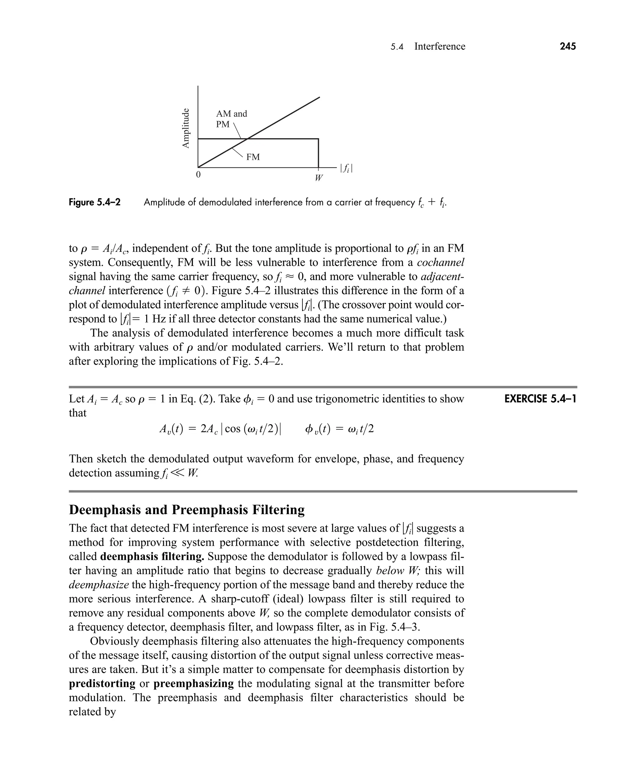
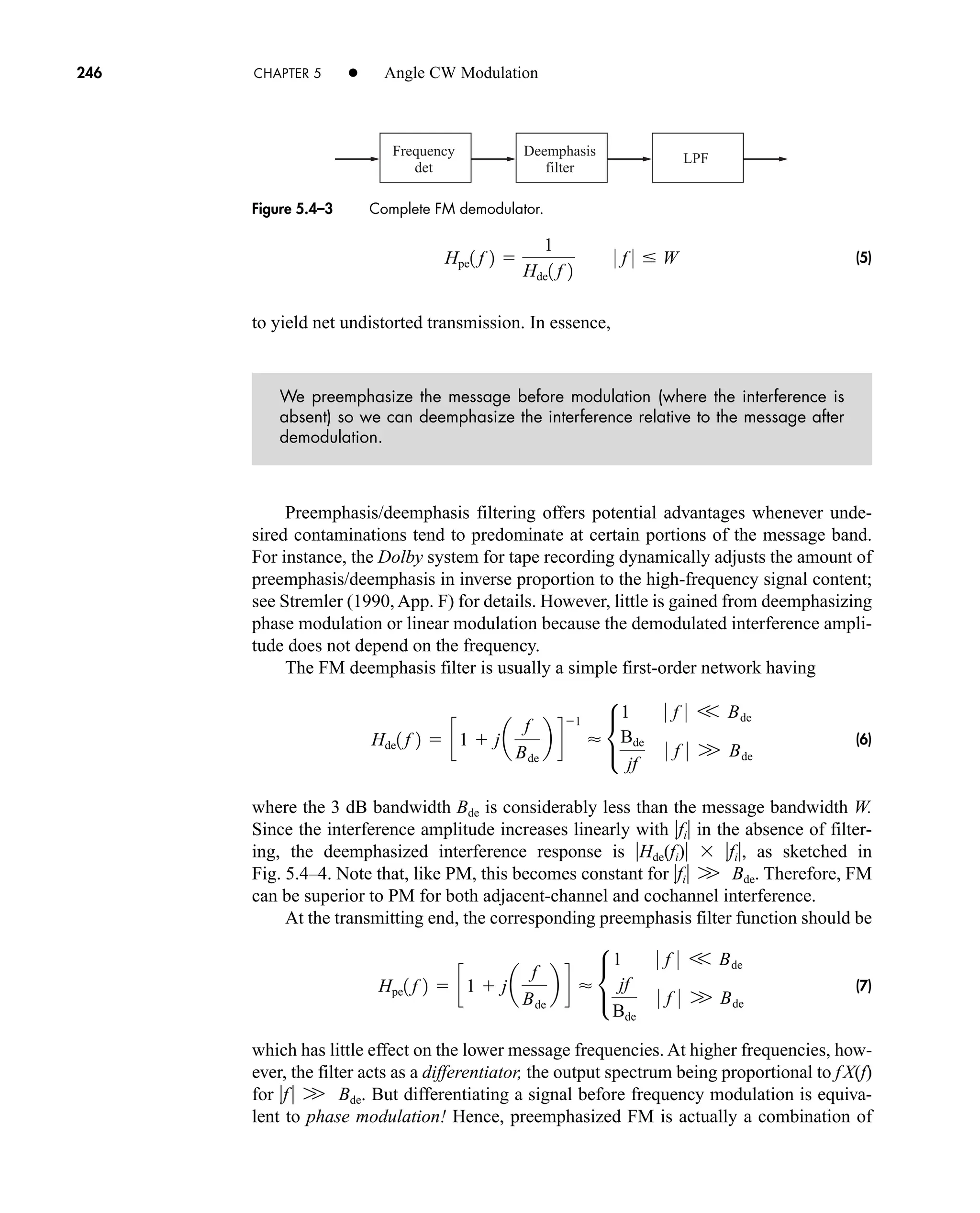
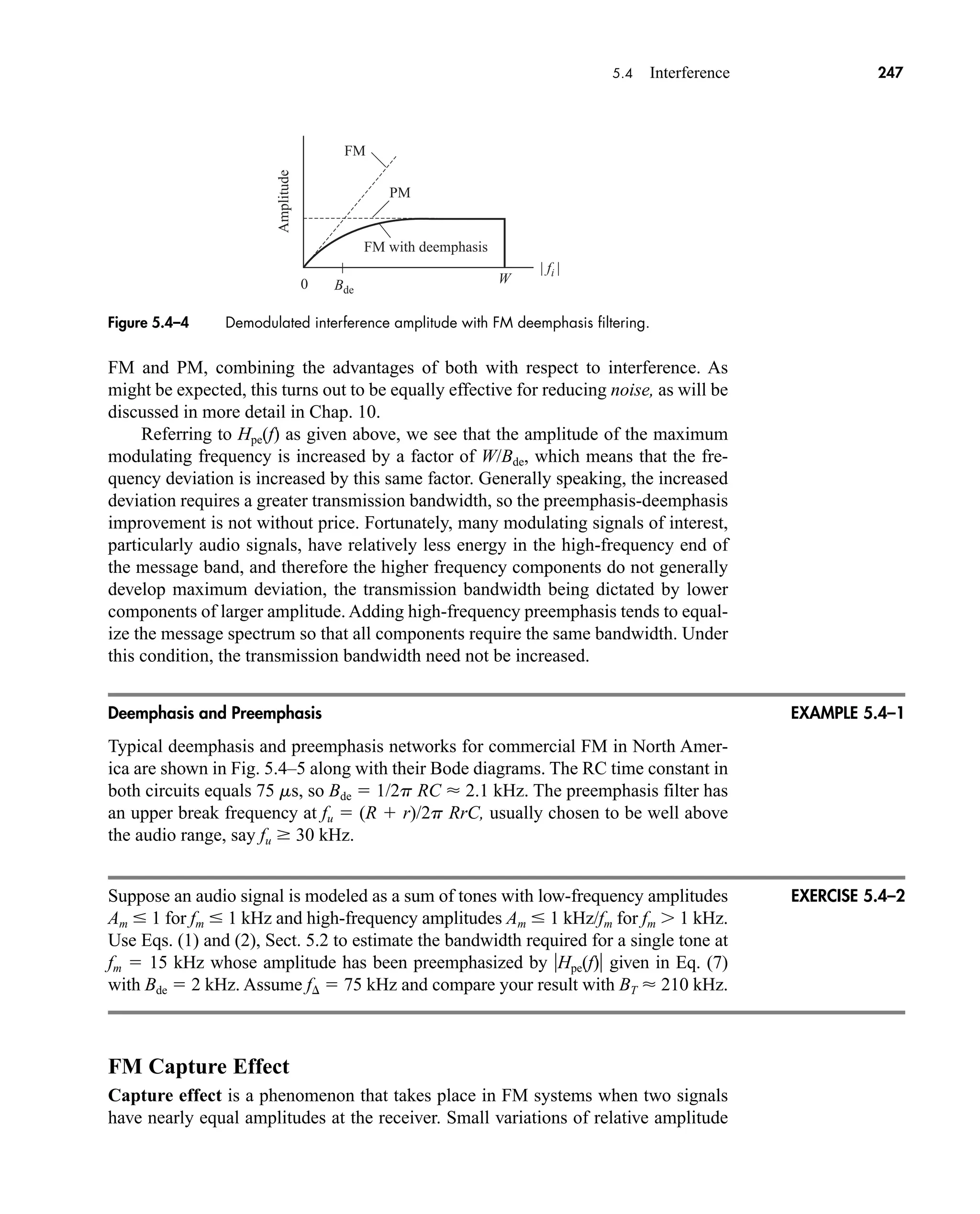
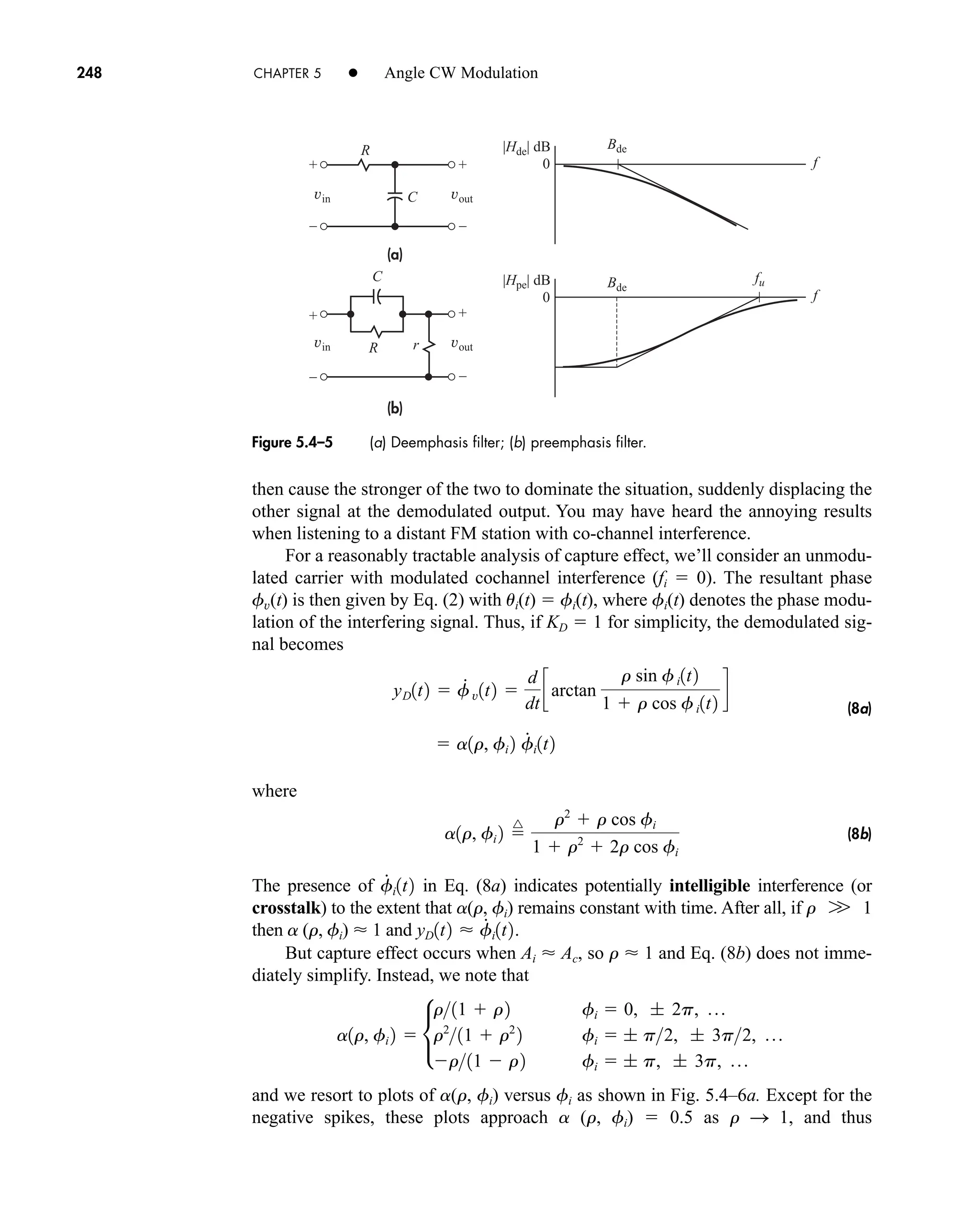
5.4 Interference 243
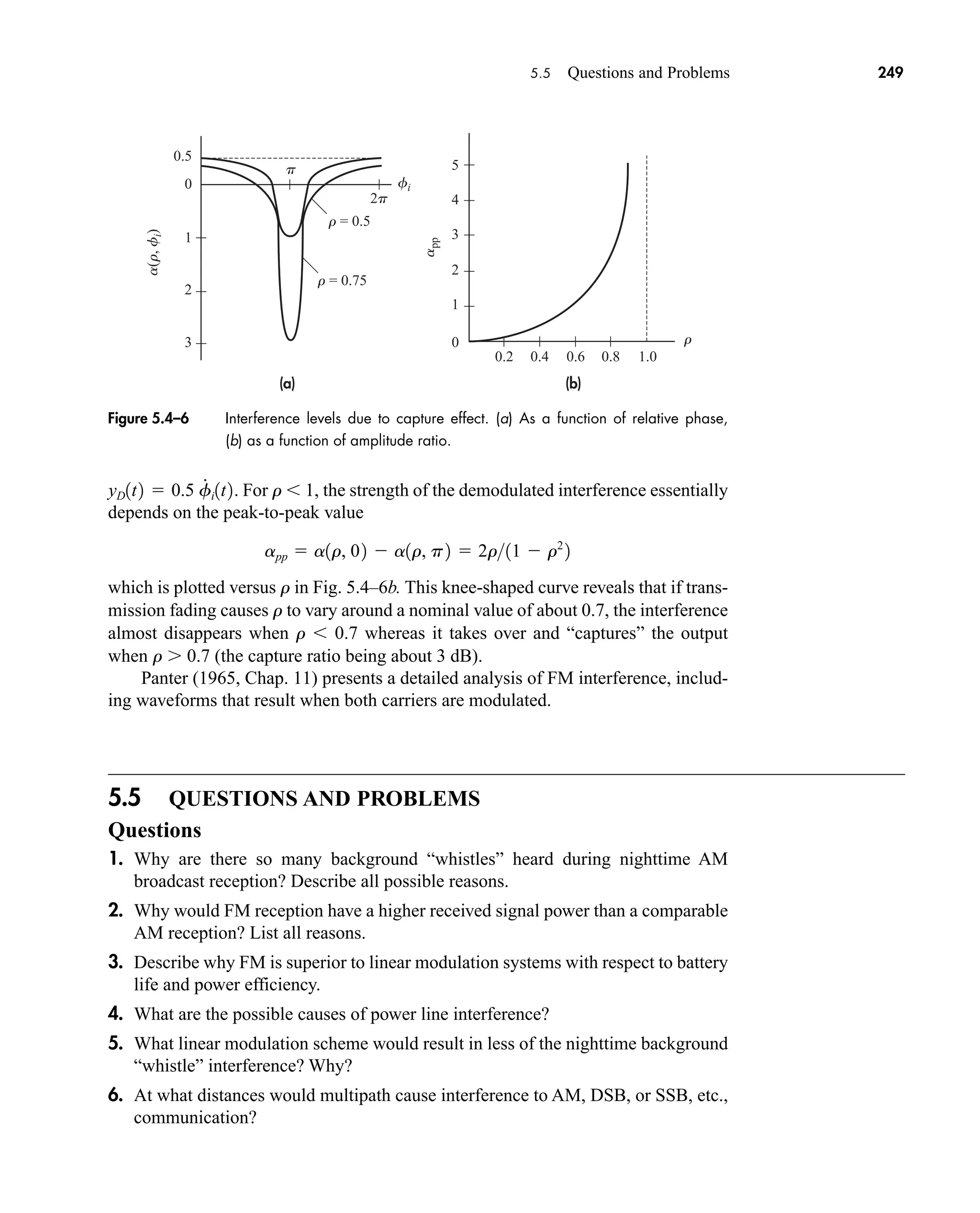
5.4 INTERFERENCE
Interference refers to the contamination of an information-bearing signal by another
similar signal, usually from a human source. This occurs in radio communication
when the receiving antenna picks up two or more signals in the same frequency
band. Interference may also result from multipath propagation, or from electromag-
netic coupling between transmission cables. Regardless of the cause, severe interfer-
ence prevents successful recovery of the message information.
Our study of interference begins with the simple but nonetheless informative
case of interfering sinusoids, representing unmodulated carrier waves. This simpli-
fied case helps bring out the differences between interference effects in AM, FM,
and PM. Then we’ll see how the technique of deemphasis filtering improves FM
performance in the face of interference. We conclude with a brief examination of the
FM capture effect.
Interfering Sinusoids
Consider a receiver tuned to some carrier frequency fc. Let the total received sig-
nal be
The first term represents the desired signal as an unmodulated carrier, while the sec-
ond term is an interfering carrier with amplitude Ai, frequency fc fi, and relative
phase angle fi.
To put v(t) in the envelope-and-phase form v(t) Av(t) cos [vct fv(t)], we’ll
introduce
(1)
r
^
AiAc ui1t2
^
vit fi
v1t2 Ac cos vc t Ai cos 31vc vi 2t fi 4
Figure 5.3–10 Zero-crossing detector: (a) diagram; (b) waveforms.
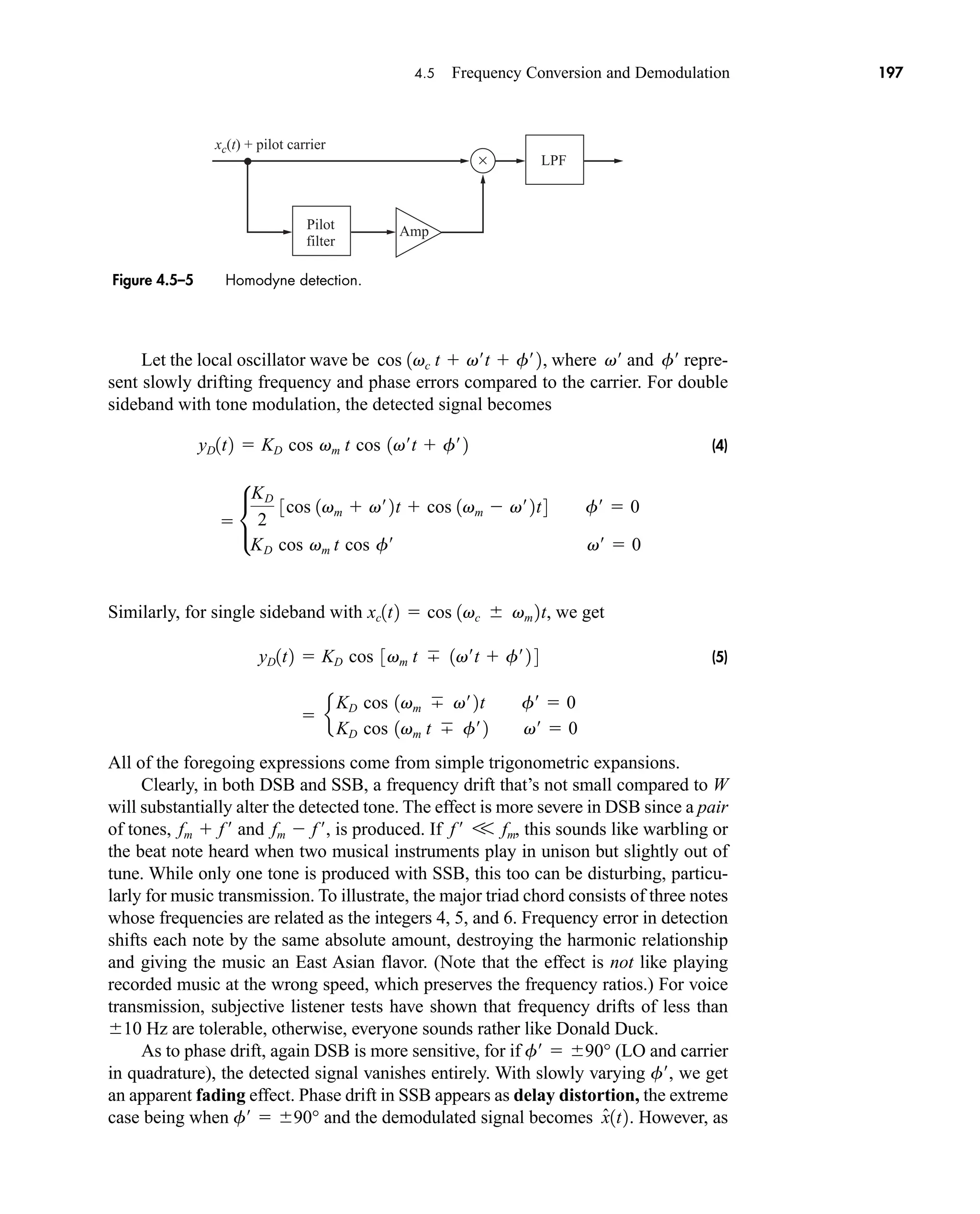
car80407_ch05_207-256.qxd 12/8/08 10:49 PM Page 243](https://image.slidesharecdn.com/communicationsystemsanintro-a-241115060943-61721fa8/75/Communication_Systems__An_Intro_-_A-_Bruce_Carlson_-pdf-265-2048.jpg)
![Av(t)
fv(t) ui(t)
Ac r sin ui(t)
Ac [1 + r cos ui(t)]
Ac
rAc
244 CHAPTER 5 • Angle CW Modulation
Hence, Ai rAc and the phasor construction in Fig. 5.4–1 gives
(2)
These expressions show that interfering sinusoids produce both amplitude and phase
modulation. In fact, if r V 1 then
(3)
which looks like tone modulation at frequency fi with AM modulation index m r
and FM or PM modulation index b r. At the other extreme, if r 1 then
so the envelope still has tone modulation but the phase corresponds to a shifted car-
rier frequency fc fi plus the constant fi.
Next we investigate what happens when v(t) is applied to an ideal envelope,
phase, or frequency demodulator with detection constant KD. We’ll take the weak
interference case (r V 1) and use the approximation in Eq. (3) with fi 0. Thus,
the demodulated output is
(4)
provided that fi W—otherwise, the lowpass filter at the output of the demodulator
would reject fi W. The constant term in the AM result would be removed if the
demodulator includes a DC block. As written, this result also holds for synchronous
detection in DSB and SSB systems since we’ve assumed fi 0. The multiplicative
factor fi in the FM result comes from the instantaneous frequency deviation .
Equation (4) reveals that weak interference in a linear modulation system or phase
modulation system produces a spurious output tone with amplitude proportional
f
#
y1t22p
yD1t2 •
KD 11 r cos vit2 AM
KD r sin vit PM
KD r fi cos vit FM
fv1t2 vi t fi
Av1t2 Ai 31 r1
cos 1vi t fi 2 4
W
fv1t2 r sin 1vi t fi 2
Av1t2 Ac 31 r cos 1vi t fi 2 4
f v1t2 arctan
r sin ui1t2
1 r cos ui1t2
Av1t2 Ac 21 r2
2r cos ui1t2
Figure 5.4–1 Phasor diagram of interfering carriers.
car80407_ch05_207-256.qxd 12/8/08 10:49 PM Page 244](https://image.slidesharecdn.com/communicationsystemsanintro-a-241115060943-61721fa8/75/Communication_Systems__An_Intro_-_A-_Bruce_Carlson_-pdf-266-2048.jpg)
![252 CHAPTER 5 • Angle CW Modulation
5.2–3 What is the maximum frequency deviation for a FM system where
W 3 kHz and BT 30 kHz?
5.2–4 Do Prob. 5.2–3 with BT 10 kHz?
5.2–5 An FM system has f 10 kHz. Use Table 9.4–1 and Fig. 5.2–1 to estimate
the bandwidth for: (a) barely intelligible voice transmission; (b) telephone-
quality voice transmission: (c) high-fidelity audio transmission.
5.2–6 A video signal with W 5 MHz is to be transmitted via FM with
f 25 MHz. Find the minimum carrier frequency consistent with frac-
tional bandwidth considerations. Compare your results with transmis-
sion via DSB amplitude modulation.
5.2–7* Your new wireless headphones use infrared FM transmission and have a
frequency response of 30–15,000 Hz. Find BT and f consistent with
fractional bandwidth considerations, assuming fc 5 1014
Hz.
5.2–8 A commercial FM radio station alternates between music and talk
show/call-in formats. The broadcasted CD music is bandlimited to 15 kHz
based on convention. Assuming D 5 is used for both music and voice,
what percentage of the available transmission bandwidth is used during
the talk show if we take W 5 kHz for voice signals?
5.2–9 An FM system with f 30 kHz has been designed for W 10 kHz.
Approximately what percentage of BT is occupied when the modulating
signal is a unit-amplitude tone at fm 0.1, 1.0, or 5.0 kHz? Repeat your
calculations for a PM system with f 3 rad.
5.2–10 Consider phase-integral and phase-acceleration modulation defined in
Prob. 5.1–5. Investigate the bandwidth requirements for tone modula-
tion, and obtain transmission bandwidth estimates. Discuss your results.
5.2–11* The transfer function of a single-tuned BPF is H(f) 1/[1 j2Q (f fc)/fc]
over the positive-frequency passband. Use Eq. (10) to obtain an expression
for the output signal and its instantaneous phase when the input is an
NBPM signal.
5.2–12 Use Eq. (10) to obtain an expression for the output signal and its ampli-
tude when an FM signal is distorted by a system having H(f) K0
K3(f fc)3
over the positive-frequency passband.
5.2–13 Use Eq. (13) to obtain an expression for the output signal and its instan-
taneous frequency when an FM signal is distorted by a system having
H(f) 1 and arg H(f) a1(f fc) a3(f fc)3
over the positive-
frequency passband.
5.2–14 An FM signal is applied to the BPF in Prob. 5.2–11. Let
a 2Qf/fc V 1 and use Eq. (13) to obtain an approximate expression
for the output signal and its instantaneous frequency.
5.2–15 Let the input to the system in Fig. 5.2–6a be an FM signal with
D f/W and spurious amplitude variations. Sketch the spectrum at the
car80407_ch05_207-256.qxd 12/8/08 10:49 PM Page 252](https://image.slidesharecdn.com/communicationsystemsanintro-a-241115060943-61721fa8/75/Communication_Systems__An_Intro_-_A-_Bruce_Carlson_-pdf-274-2048.jpg)
![254 CHAPTER 5 • Angle CW Modulation
5.3–9 Suppose the phase modulator in Fig. 5.3–5 is implemented as in
Fig. 5.3–3. Take x(t) Am cos vmt and let b (f/2p T)(Am/fm).
(a) Show that if b V 1, then
(b) Obtain a condition on f/2p T so the third-harmonic distortion does
not exceed 1 percent when Am 1 and 30 Hz fm 15 kHz, as in FM
broadcasting.
5.3–10 Let the input to Fig. 5.3–7a be an FM signal with f V fc and let the differ-
entiator be implemented by a tuned circuit with H(f) 1/[1 j(2Q/f0)
(f f0)] for f f0. Use the quasi-static method to show that yD(t) KD f x(t)
when f0 fc b provided that f V b V f0/2Q.
5.3–11* Let the input to Fig. 5.3–7a be an FM signal with f V fc and let the dif-
ferentiator be implemented by a first-order lowpass filter with B fc. Use
quasi-static analysis to show that yD1t2 K1 f¢x1t2 K2 f ¢
2
x2
1t2.
f11t2 fc bfm 3cos vmt 1b222
cos 3vmt4
Then take x(t) cos vmt and obtain a condition on f/fc so the second-
harmonic distortion is less than 1%.
5.3–12 The tuned circuits in Fig. 5.3–8b have transfer functions of the form
H(f) 1/[1 j(2Q/f0)(f f0] for f f0). Let the two center frequencies
be f0 fc b with f b V fc. Use quasi-static analysis to show that if
both circuits have (2Q/f0)b a V 1, then yD(t) K1x(t) K3x3
(t)
where K3/K1 V 1.
5.3–13 You have been given an NBFM exciter with fc 7 MHz, W 2.5 kHz,
and f 1.25 kHz. Using a series of frequency doublers and triplers and
possibly a heterodyne stage, design a converter that will enable a WBFM
signal with fc 220 MHz, and f 15 kHz. Justify your results.
5.3–14 Given a NBFM exciter with fc 8 MHz, W 3 kHz, f 0.3 kHz,
using frequency triplers and heterodyning units, design an FM system
with fc 869–894 MHz and BT 30 kHz.
5.4–1 Obtain an approximate expression for the output of an amplitude
demodulator when the input is an AM signal with 100 percent modula-
tion plus an interfering signal Ai[1 xi(t)] cos [(vc vi)t fi] with
r Ai/Ac V 1. Is the demodulated interference intelligible?
5.4–2 Obtain an approximate expression for the output of a phase demodulator
when the input is an NBPM signal with 100 percent modulation plus an
interfering signal Ai cos [(vc vi)t fi(t)] with r Ai/Ac V 1. Is the
demodulated interference intelligible?
5.4–3 Investigate the performance of envelope detection versus synchronous
detection of AM in the presence of multipath propagation, so that
v(t) xc(t) axc(t td) with a2
1. Consider the special cases
vctd p/2 and vctd p.
car80407_ch05_207-256.qxd 12/8/08 10:49 PM Page 254](https://image.slidesharecdn.com/communicationsystemsanintro-a-241115060943-61721fa8/75/Communication_Systems__An_Intro_-_A-_Bruce_Carlson_-pdf-276-2048.jpg)
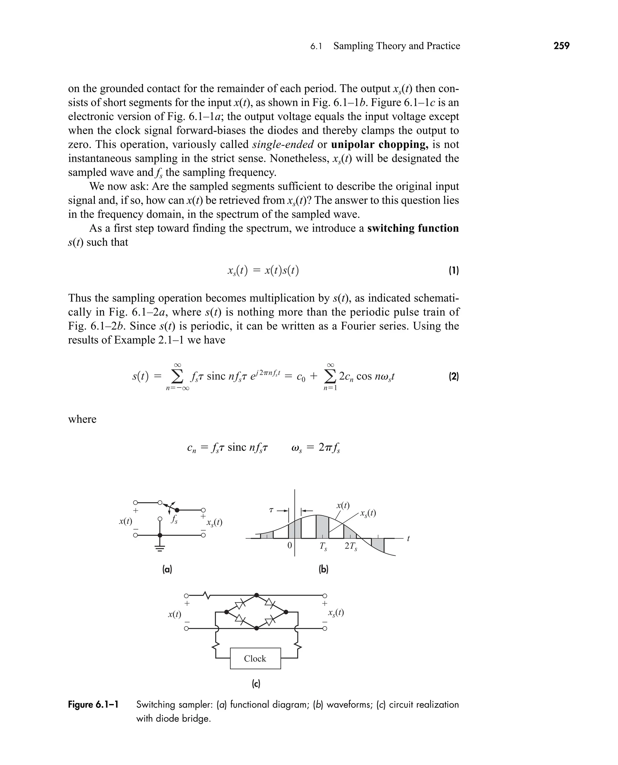
![(b)
(a)
xs(t) = x(t)s(t)
x(t)
s(t)
s(t)
t
Ts
t
×
Figure 6.1–2 Sampling as multiplication: (a) functional diagram; (b) switching function.
260 CHAPTER 6 • Sampling and Pulse Modulation
Combining Eq. (2) with Eq. (1) yields the term-by-term expansion
(3)
Thus, if the input message spectrum is X(f) [x(t)], the output spectrum is
(4)
which follows directly from the modulation theorem.
While Eq. (4) appears rather messy, the spectrum of a sampled wave is readily
sketched if the input signal is assumed to be bandlimited. Figure 6.1–3 shows a con-
venient X(f) and the corresponding Xs(f) for two cases, fs 2W and fs 2W. This fig-
ure reveals something quite surprising: The sampling operation has left the message
spectrum intact, merely repeating it periodically in the frequency domain with a
spacing of fs. We also note that the first term of Eq. (4) is precisely the message spec-
trum, attenuated by the duty cycle c0 fst t/Ts.
If sampling preserves the message spectrum, it should be possible to recover or
reconstruct x(t) from the sampled wave xs(t). The reconstruction technique is not at
all obvious from the time-domain relations in Eqs. (1) and (3). But referring again to
Fig. 6.1–3, we see that X(f) can be separated from Xs(f) by lowpass filtering, pro-
vided that the spectral sidebands don’t overlap. And if X(f) alone is filtered from
Xs(f), we have recovered x(t). Two conditions obviously are necessary to prevent
overlapping spectral bands: the message must be bandlimited, and the sampling fre-
quency must be sufficiently great that fs – W W. Thus we require
and
(5a)
If the sampled signal is sinusoidal, its frequency spectrum will consist of impulses
and equality of Eq. (5a) does not hold, and we thus require
fs 2W or Ts
1
2W
X1 f 2 0 0 f 0 7 W
Xs1 f 2 c0 X1 f 2 c1 3X1 f fs 2 X1 f fs 2 4
c2 3X1 f 2fs 2 X1 f 2fs 2 4
p
xs 1t2 c0 x1t2 2c1x1t2 cos vst 2c2 x1t2 cos 2vst p
car80407_ch06_257-286.qxd 12/8/08 11:41 PM Page 260](https://image.slidesharecdn.com/communicationsystemsanintro-a-241115060943-61721fa8/75/Communication_Systems__An_Intro_-_A-_Bruce_Carlson_-pdf-282-2048.jpg)
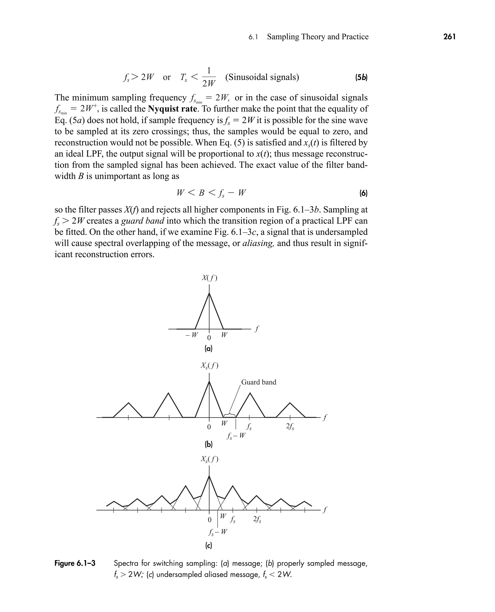
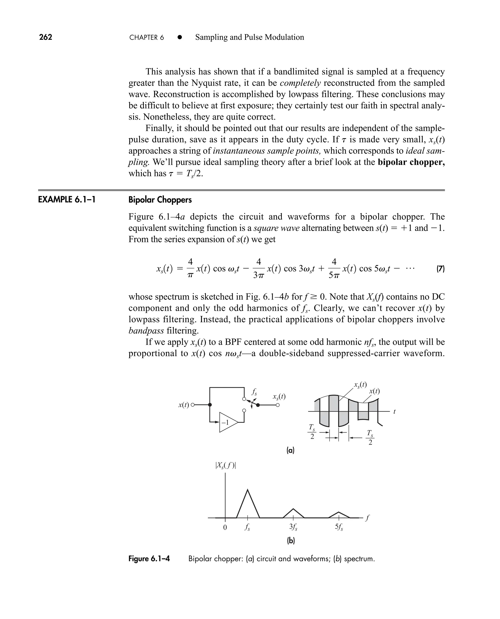
![6.1 Sampling Theory and Practice 263
Thus, a bipolar chopper serves as a balanced modulator. It also serves as a
synchronous detector when the input is a DSB or SSB signal and the output is
lowpass filtered. These properties are combined in the chopper-stabilized ampli-
fier, which makes possible DC and low-frequency amplification using a high-gain
AC amplifier. Additionally, Prob. 6.1–4 indicates how a bipolar chopper can be mod-
ified to produce the baseband multiplexed signal for FM stereo.
Ideal Sampling and Reconstruction
By definition, ideal sampling is instantaneous sampling. The switching device of
Fig. 6.1–1a yields instantaneous values only if t S 0; but then fst S 0, and so does
xs(t). Conceptually, we overcome this difficulty by multiplying xs(t) by 1/t so that, as
t S 0 and 1/t S , the sampled wave becomes a train of impulses whose areas
equal the instantaneous sample values of the input signal. Formally, we write the rec-
tangular pulse train as
from which we define the ideal sampling function
(8)
The ideal sampled wave is then
(9a)
(9b)
since x(t) d(t – kTs) x(kTs) d(t – kTs).
To obtain the corresponding spectrum Xd(f) [xd(t)] we note that
(1/t)xs(t) S xd(t) as t S 0 and, likewise, (1/t)Xs(f) S Xd(f). But each coefficient in
Eq. (4) has the property cn/t fs sinc nfst fs when t 0. Therefore,
(10)
which is illustrated in Fig. 6.1–5 for the message spectrum of Fig. 6.1–3a, taking
fs 2W. We see that Xd(f) is periodic in frequency with period fs, a crucial
observation in the study of sampled-data systems.
fs a
q
nq
X1 f nfs 2
Xd 1 f 2 fsX1 f 2 fs 3X1 f fs 2 X1 f fs 2 4 p
a
q
kq
x1kTs 2 d1t kTs 2
x1t2 a
q
kq
d1t kTs 2
xd1t2
^
x1t2sd1t2
sd1t2
^
lim
tS0
1
t
s1t2 a
q
kq
d1t kTs 2
s1t2 a
q
kq
ß a
t kTs
t
b
car80407_ch06_257-286.qxd 12/8/08 11:41 PM Page 263](https://image.slidesharecdn.com/communicationsystemsanintro-a-241115060943-61721fa8/75/Communication_Systems__An_Intro_-_A-_Bruce_Carlson_-pdf-285-2048.jpg)
![0
Xd( f )
2fs
fs – W
fs
W
f
Figure 6.1–5 Spectrum of ideally sampled message.
264 CHAPTER 6 • Sampling and Pulse Modulation
Somewhat parenthetically, we can also develop an expression for Sd(f)
[sd(t)] as follows. From Eq. (9a) and the convolution theorem, Xd(f) X(f) * Sd(f)
whereas Eq. (10) is equivalent to
Therefore, we conclude that
(11)
so the spectrum of a periodic string of unit-weight impulses in the time domain is a
periodic string of impulses in the frequency domain with spacing fs 1/Ts; in both
domains we have a function that looks like the uprights in a picket fence.
Returning to the main subject and Fig. 6.1–5, it’s immediately apparent that if
we invoke the same conditions as before—x(t) bandlimited in W and fs 2W—then
a filter of suitable bandwidth will reconstruct x(t) from the ideal sampled wave.
Specifically, for an ideal LPF of gain K, time delay td, and bandwidth B, the transfer
function is
so filtering xd(t) produces the output spectrum
assuming B satisfies Eq. (6). The output time function is then
(12)
which is the original signal amplified by Kfs and delayed by td.
Further confidence in the sampling process can be gained by examining recon-
struction in the time domain. The impulse response of the LPF is
h1t2 2BK sinc 2B1t td 2
y1t2 1
3Y1 f 2 4 Kfsx1t td 2
Y1 f 2 H1 f 2Xd1 f 2 KfsX1 f 2ejvtd
H1 f 2 Kß a
f
2B
bejvtd
Sd1 f 2 fs a
q
nq
d1 f nfs 2
Xd 1 f 2 X1 f 2 * c a
q
nq
fs d1 f nfs 2 d
car80407_ch06_257-286.qxd 12/8/08 11:41 PM Page 264](https://image.slidesharecdn.com/communicationsystemsanintro-a-241115060943-61721fa8/75/Communication_Systems__An_Intro_-_A-_Bruce_Carlson_-pdf-286-2048.jpg)
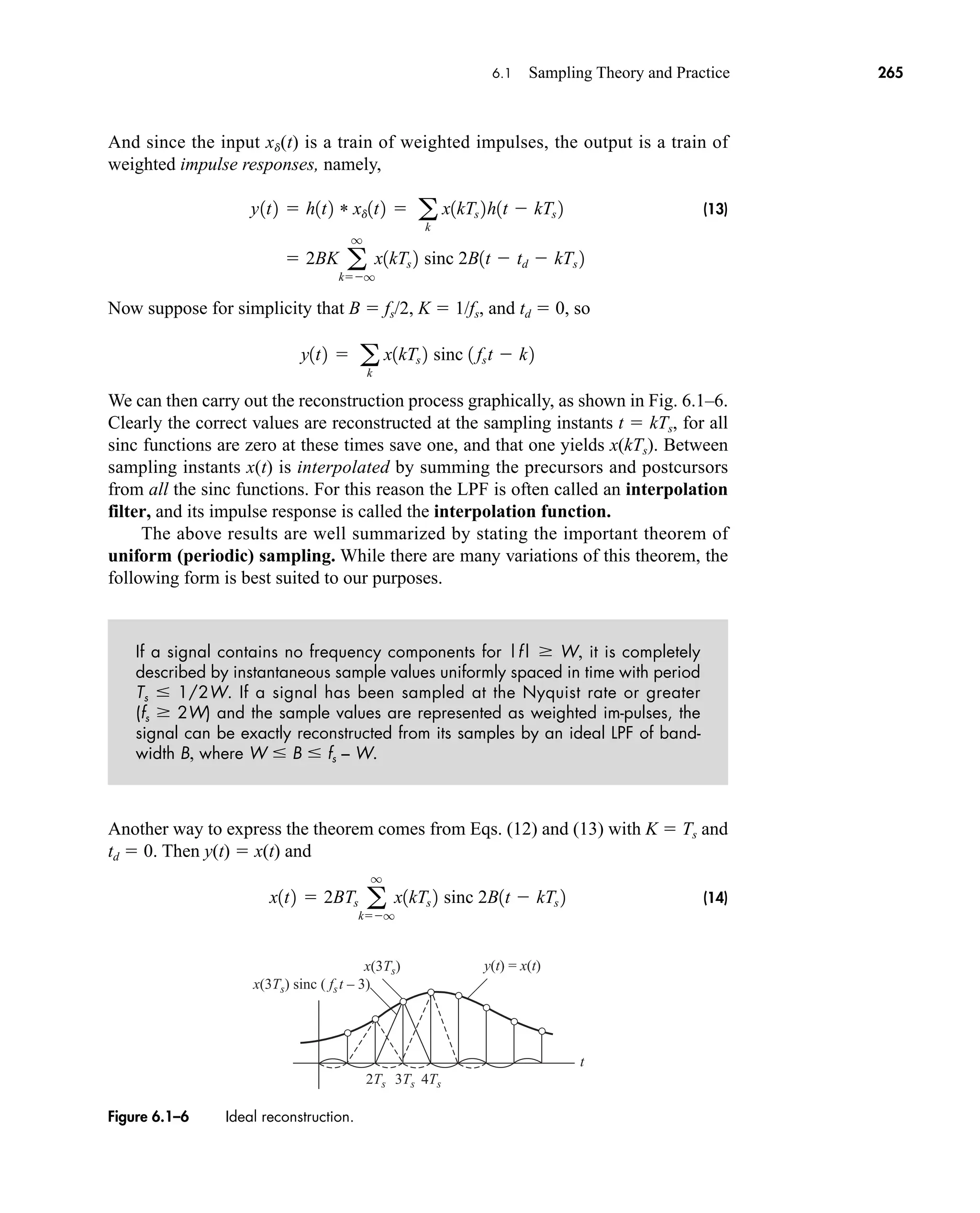
![266 CHAPTER 6 • Sampling and Pulse Modulation
provided Ts 1/2W and B satisfies Eq. (6). Therefore, just as a periodic signal is
completely described by its Fourier series coefficients, a bandlimited signal is com-
pletely described by its instantaneous sample values whether or not the signal actu-
ally is sampled.
Consider a sampling pulse train of the general form
(15a)
whose pulse type p(t) equals zero for t Ts/2 but is otherwise arbitrary. Use an
exponential Fourier series and Eq. (21), Sect. 2.2, to show that
(15b)
where P(f) [p(t)]. Then let p(t) d(t) to obtain Eq. (11).
Practical Sampling and Aliasing
Practical sampling differs from ideal sampling in three obvious aspects:
1. The sampled wave consists of pulses having finite amplitude and duration,
rather than impulses.
2. Practical reconstruction filters are not ideal filters.
3. The messages to be sampled are timelimited signals whose spectra are not and
cannot be strictly bandlimited.
The first two differences may present minor problems, while the third leads to the
more troublesome effect known as aliasing.
Regarding pulse-shape effects, our investigation of the unipolar chopper and the
results of Exercise 6.1–1 correctly imply that almost any pulse shape p(t) will do
when sampling takes the form of a multiplication operation x(t)sp(t). Another opera-
tion produces flat-top sampling described in the next section. This type of sampling
may require equalization, but it does not alter our conclusion that pulse shapes are
relatively inconsequential.
Regarding practical reconstruction filters, we consider the typical filter response
superimposed in a sampled-wave spectrum in Fig. 6.1–7. As we said earlier, recon-
struction can be done by interpolating between samples. The ideal LPF does a per-
fect interpolation. With practical systems, we can reconstruct the signal using a
zero-order hold (ZOH) with
(16)
y1t2 a
k
x1kTs 2ß a
t kTs
Ts
b
Sp1 f 2 fs a
q
nq
P1nfs 2 d1 f nfs 2
sp1t2 a
q
kq
p1t kTs 2
EXERCISE 6.1–1
car80407_ch06_257-286.qxd 12/8/08 11:41 PM Page 266](https://image.slidesharecdn.com/communicationsystemsanintro-a-241115060943-61721fa8/75/Communication_Systems__An_Intro_-_A-_Bruce_Carlson_-pdf-288-2048.jpg)
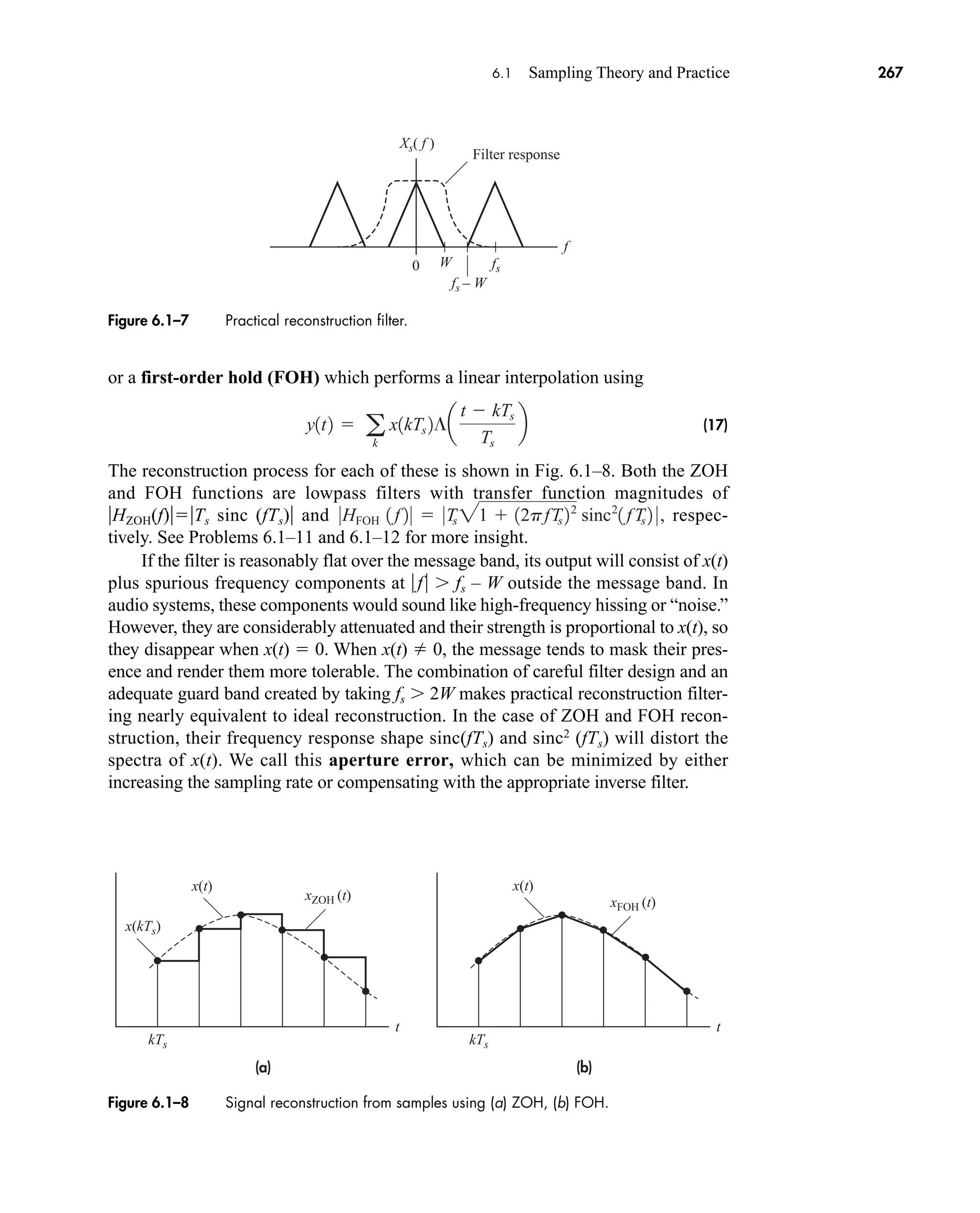
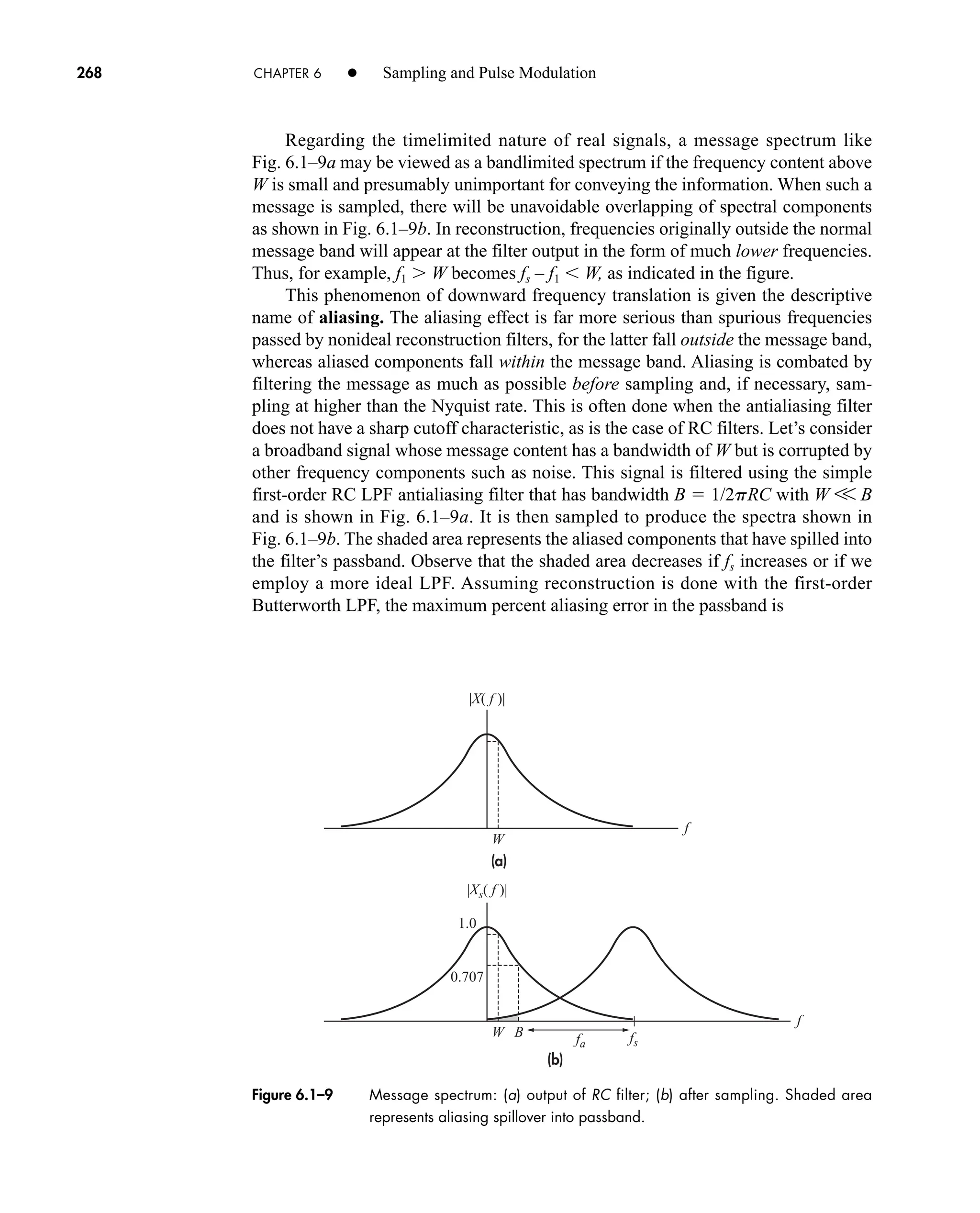
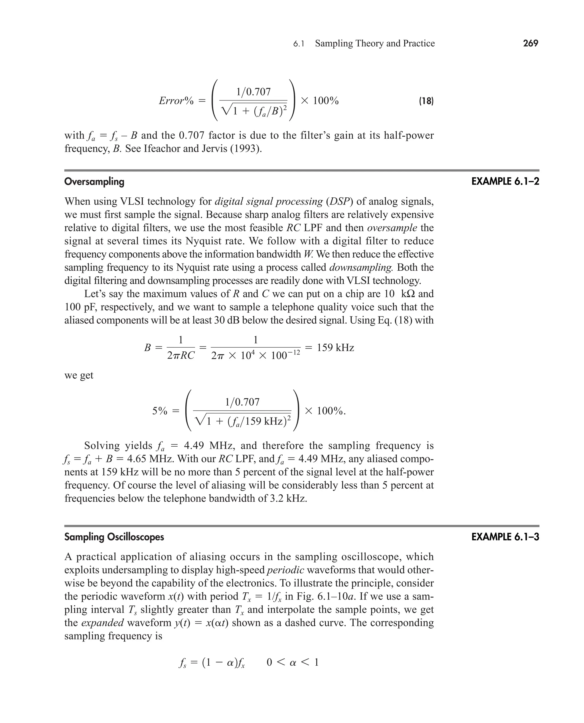
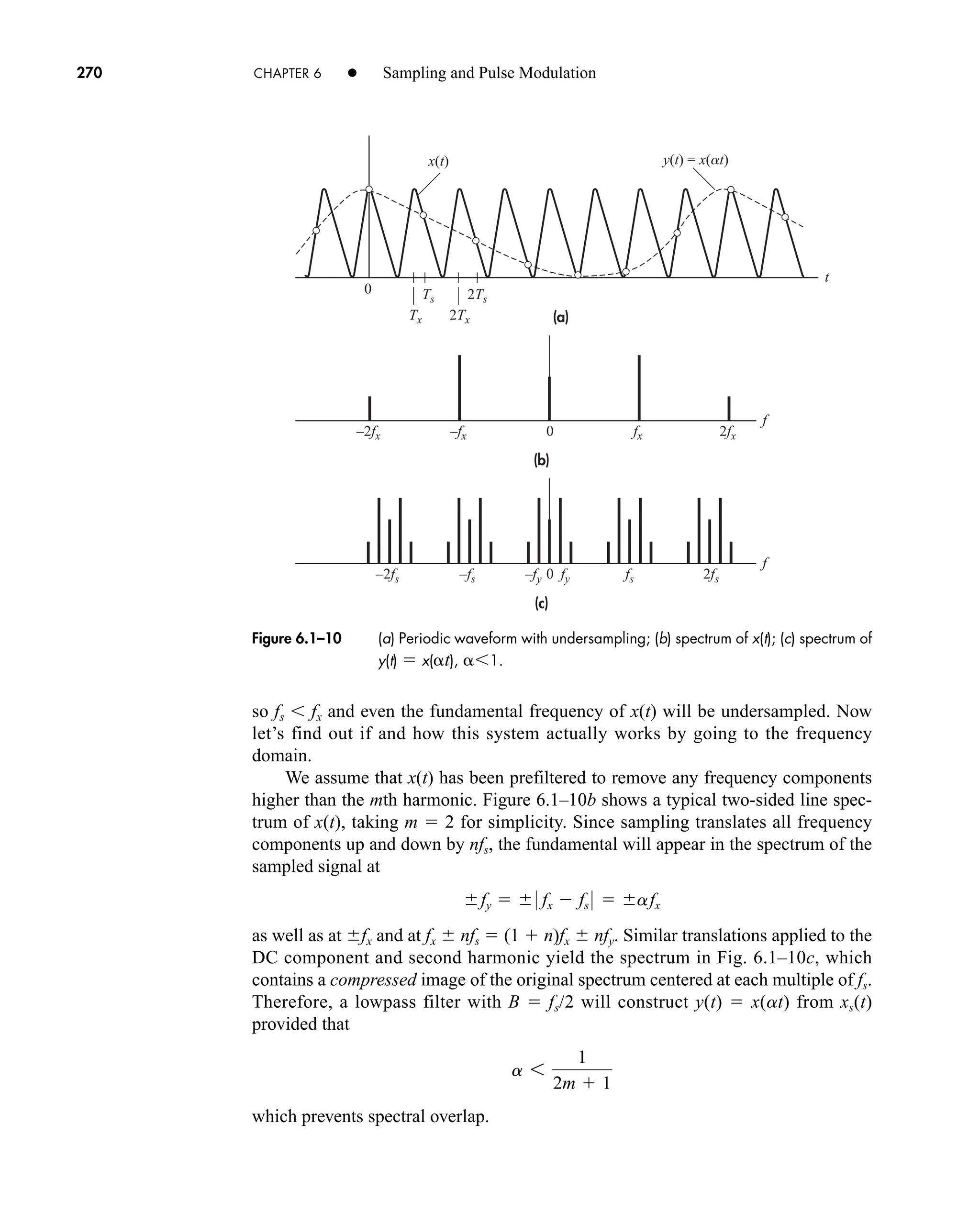
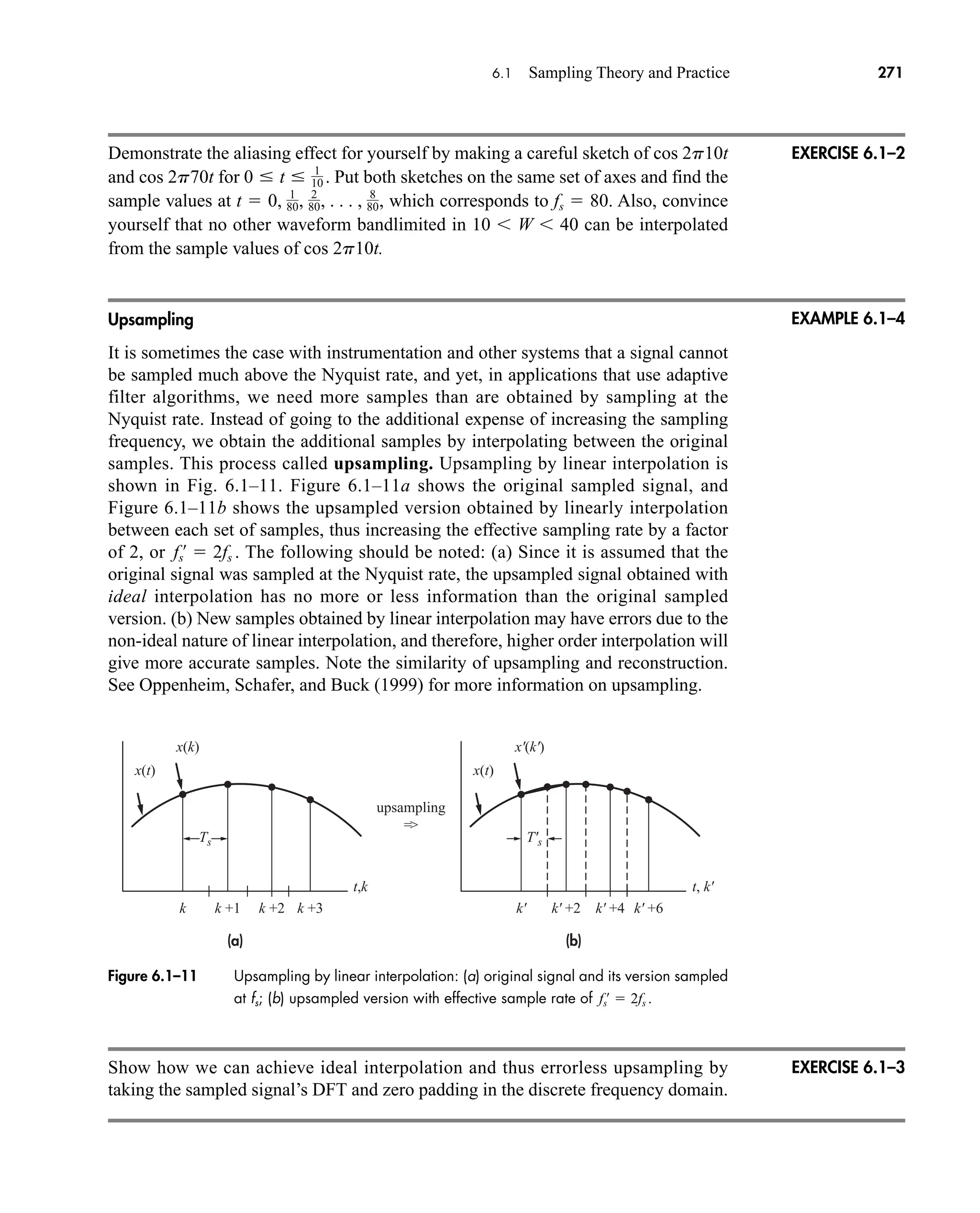
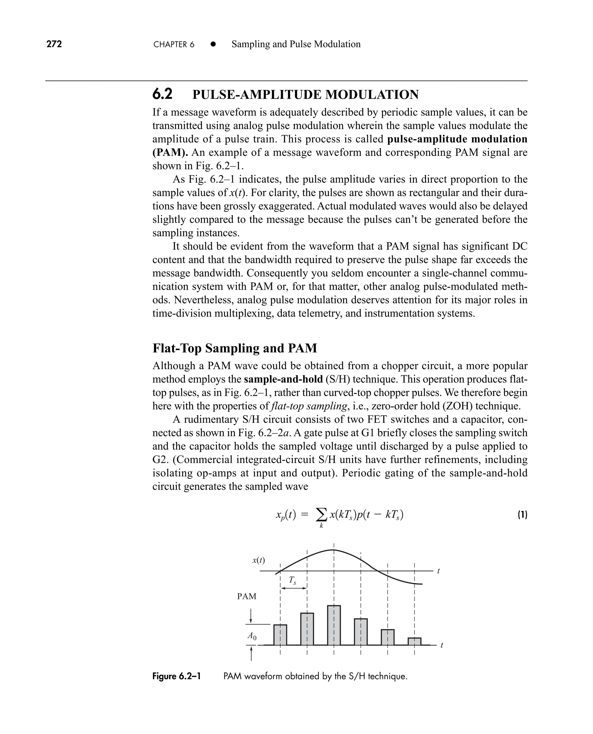
![(a) (b)
Sampling
switch
Discharge
switch
xp(t)
C
G2
G1
x(t)
x(t) x(kTs)
kTs
t
t
+
–
+
–
Figure 6.2–2 Flat-top sampling: (a) sample-and-hold circuit; (b) waveforms.
(a)
(b)
0 fs
f
0 fs
– fs
– fs
f
|Xd( f )|
|Xp( f )|
|P( f )|
Figure 6.2–3 (a) Spectrum for ideal sampling when X(f) Π (f/2W); (b) aperture effect in
flat-top sampling.
6.2 Pulse-Amplitude Modulation 273
illustrated by Fig. 6.2–2b. Note that each output pulse of duration t represents a sin-
gle instantaneous sample value.
To analyze flat-top sampling, we’ll draw upon the relation p(t – kTs)
p(t) * d(t – kTs) and write
Fourier transformation of this convolution operation yields
(2)
Figure 6.2–3 provides a graphical interpretation of Eq. (2), taking X(f) Π (f/2W).
We see that flat-top sampling is equivalent to passing an ideal sampled wave through
a network having the transfer function P(f) [p(t)].
Xp1 f 2 P1 f 2 c fs a
n
X1 f nfs 2 d P1 f 2Xd1 f 2
xp1t2 p1t2 * c a
k
x1kTs 2 d1t kTs 2 d p1t2 * xd1t2
car80407_ch06_257-286.qxd 12/8/08 11:41 PM Page 273](https://image.slidesharecdn.com/communicationsystemsanintro-a-241115060943-61721fa8/75/Communication_Systems__An_Intro_-_A-_Bruce_Carlson_-pdf-295-2048.jpg)
![274 CHAPTER 6 • Sampling and Pulse Modulation
The high-frequency rolloff characteristic of a typical P(f) acts like a lowpass
filter and attenuates the upper portion of the message spectrum. This loss of high-
frequency content is called aperture effect. The larger the pulse duration or aperture
t, the larger the effect. Aperture effect can be corrected in reconstruction by includ-
ing an equalizer with
(3)
However, little if any equalization is needed when t/Ts V 1.
Now consider a unipolar flat-top PAM signal defined by
(4)
The constant A0 equals the unmodulated pulse amplitude, and the modulation index
m controls the amount of amplitude variation. The condition
(5)
ensures a unipolar (single-polarity) waveform with no missing pulses. The resulting
constant pulse rate fs is particularly important for synchronization in time-division
multiplexing.
Comparison of Eqs. (1) and (4) shows that a PAM signal can be obtained from a
sample-and-hold circuit with input A0[1 mx(t)]. Correspondingly, the PAM
spectrum will look like Fig. 6.2–3b with X(f) replaced by
which results in spectral impulses at all harmonics of fs and at f 0. Reconstruction
of x(t) from xp(t) therefore requires a DC block as well as lowpass filtering and equal-
ization.
Clearly, PAM has many similarities to AM CW modulation—modulation index,
spectral impulses, and dc blocks. (In fact, an AM wave could be derived from PAM
by bandpass filtering). But the PAM spectrum extends from DC up through several
harmonics of fs, and the estimate of required transmission bandwidth BT must be
based on time-domain considerations. For this purpose, we assume a small pulse
duration t compared to the time between pulses, so
Adequate pulse resolution then requires
(6)
Hence, practical applications of PAM are limited to those situations in which the
advantages of a pulsed waveform outweigh the disadvantages of large bandwidth.
BT
1
2t
W W
t V Ts
1
2W
5A0 31 mx1t2 46 A0 3d1 f 2 mX1 f 2 4,
1 mx1t2 7 0
xp1t2 a
k
A0 31 mx1kTs 2 4 p1t kTs 2
Heq1 f 2 Kejvtd
P1 f 2
car80407_ch06_257-286.qxd 12/8/08 11:41 PM Page 274](https://image.slidesharecdn.com/communicationsystemsanintro-a-241115060943-61721fa8/75/Communication_Systems__An_Intro_-_A-_Bruce_Carlson_-pdf-296-2048.jpg)
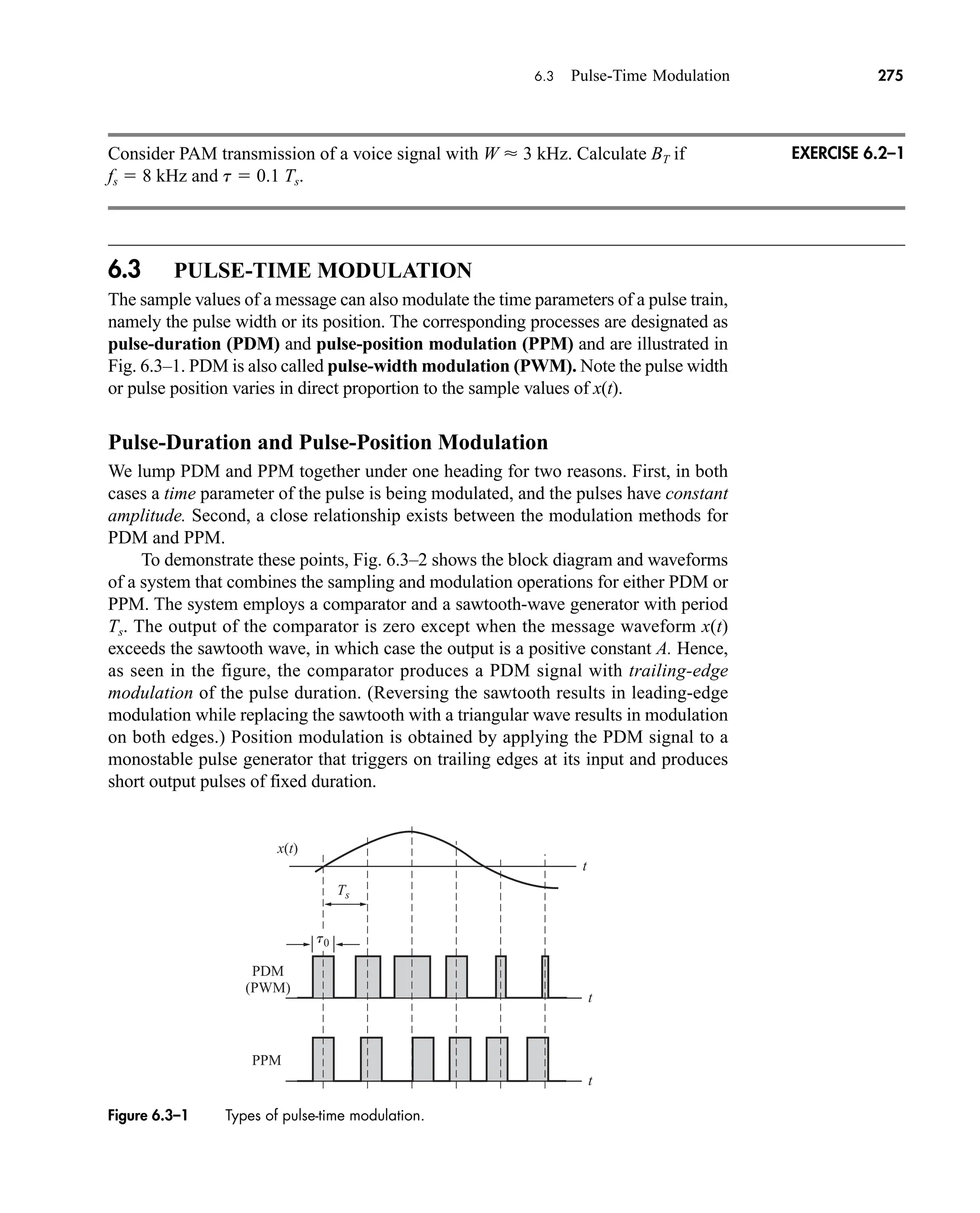
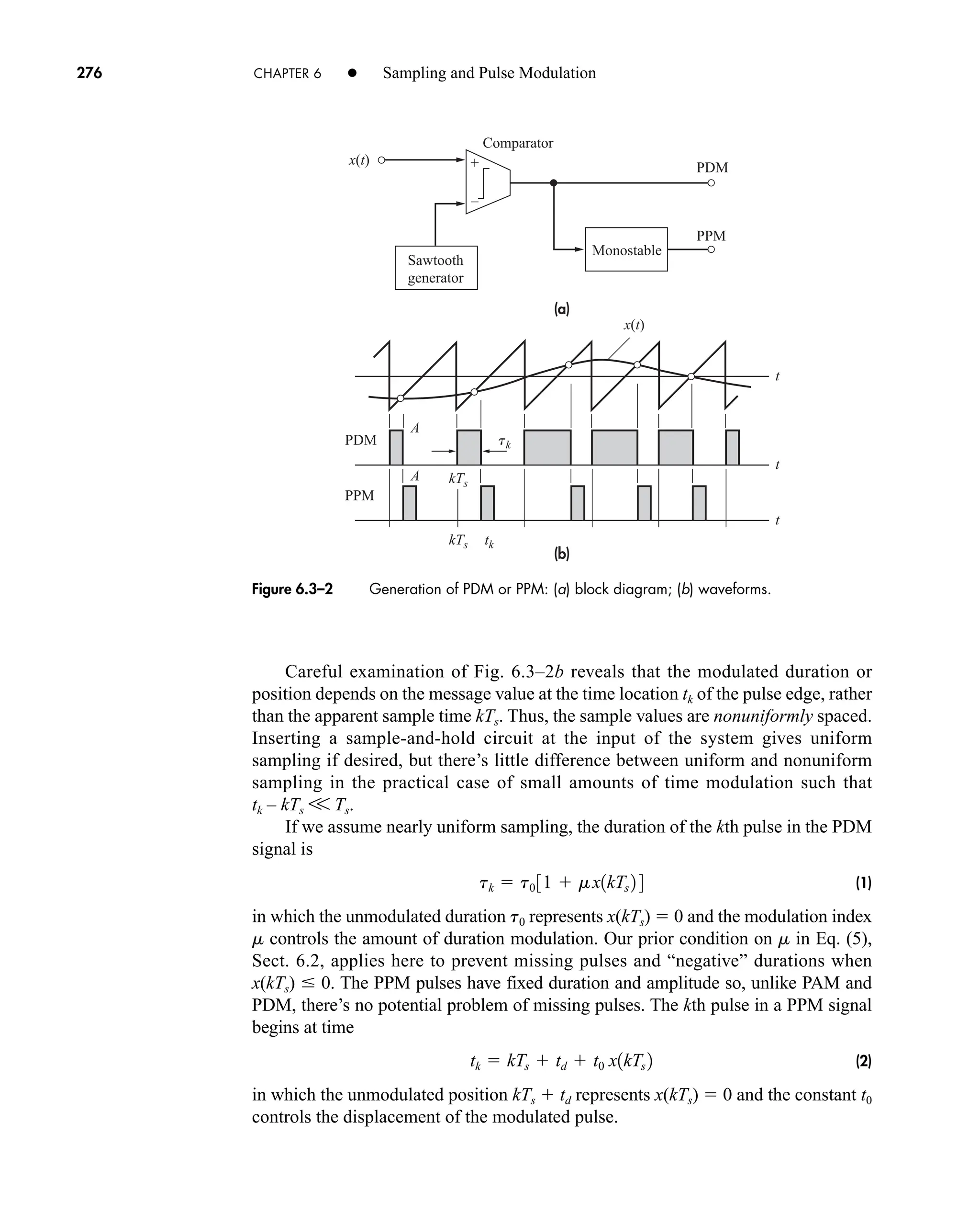
![t
t
t
tk
kTs (k + 1)Ts
PDM
PPM
Figure 6.3–3 Conversion of PDM or PPM into PAM.
6.3 Pulse-Time Modulation 277
The variable time parameters in Eqs. (1) and (2) make the expressions for xp(t)
rather awkward. However, an informative approximation for the PDM waveform is
derived by taking rectangular pulses with amplitude A centered at t kTs and assum-
ing that tk varies slowly from pulse to pulse. Series expansion then yields
(3)
where f(t) pfst0[1 mx(t)]. Without attempting to sketch the corresponding
spectrum, we see from Eq. (3) that the PDM signal contains the message x(t) plus a
DC component and phase-modulated waves at the harmonics of fs. The phase modu-
lation has negligible overlap in the message band when t0 V Ts, so x(t) can be
recovered by lowpass filtering with a DC block.
Another message reconstruction technique converts pulse-time modulation into
pulse-amplitude modulation, and works for PDM and PPM. To illustrate this technique
the middle waveform in Fig. 6.3–3 is produced by a ramp generator that starts at time
kTs, stops at tk, restarts at (k 1)Ts, and so forth. Both the start and stop commands can
be extracted from the edges of a PDM pulse, whereas PPM reconstruction must have
an auxiliary synchronization signal for the start command.
Regardless of the particular details, demodulation of PDM or PPM requires
received pulses with short risetime in order to preserve accurate message information.
For a specified risetime tr V Ts, the transmission bandwidth must satisfy
(4)
which will be substantially greater than the PAM transmission bandwidth. In
exchange for the extra bandwidth, we gain the benefit of constant-amplitude pulses
that suffer no ill effects from nonlinear distortion in transmission since nonlinear
distortion does not appreciably alter pulse duration or position.
Additionally, like PM and FM CW modulation, PDM and PPM have the
potential for wideband noise reduction—a potential more fully realized by PPM than
by PDM. To appreciate why this is so, recall that the information resides in the time
BT
1
2tr
xp1t2 Afs t0 31 mx1t2 4 a
q
n1
2A
pn
sin nf1t2 cos nvst
car80407_ch06_257-286.qxd 12/8/08 11:41 PM Page 277](https://image.slidesharecdn.com/communicationsystemsanintro-a-241115060943-61721fa8/75/Communication_Systems__An_Intro_-_A-_Bruce_Carlson_-pdf-299-2048.jpg)
![278 CHAPTER 6 • Sampling and Pulse Modulation
location of the pulse edges, not in the pulses themselves. Thus, somewhat like the
carrier-frequency power of AM, the pulse power of pulse-time modulation is
“wasted” power, and it would be more efficient to suppress the pulses and just trans-
mit the edges! Of course we cannot transmit edges without transmitting pulses to
define them. But we can send very short pulses indicating the position of the edges,
a process equivalent to PPM. The reduced power required for PPM is a fundamental
advantage over PDM, an advantage that becomes more apparent when we examine
the signal-to-noise ratios. Thus PAM is somewhat similar to analog AM, whereas
PDM and PWM correspond to FM.
Derive Eq. (3) by the following procedure. First, assume constant pulse duration t,
and write xp(t) As(t) with s(t) given by Eq. (2), Sect. 6.1. Then apply the quasi-
static approximation t t0[1 m x(t)].
PPM Spectral Analysis
Because PPM with nonuniform sampling is the most efficient type of analog pulse
modulation for message transmission, we should take the time to analyze its spec-
trum. The analysis method itself is worthy of examination.
Let the kth pulse be centered at time tk. If we ignore the constant time delay td in
Eq. (2), nonuniform sampling extracts the sample value at tk, rather than kTs, so
(5)
By definition, the PPM wave is a summation of constant-amplitude position-modulated
pulses, and can be written as
where A is the pulse amplitude and p(t) the pulse shape. A simplification at this point
is made possible by noting that p(t) will (or should) have a very small duration com-
pared to Ts. Hence, for our purposes, the pulse shape can be taken as impulsive, and
(6)
If desired, Eq. (6) can later be convolved with p(t) to account for the nonimpulsive
shape.
In their present form, Eqs. (5) and (6) are unsuited to further manipulation; the
trouble is the position term tk, which cannot be solved for explicitly. Fortunately, tk
can be eliminated entirely. Consider any function g(t) having a single first-order zero
xp1t2 A a
k
d1t tk 2
xp1t2 a
k
Ap1t tk 2 Ap1t2 * c a
k
d1t tk 2 d
tk kTs t0 x1tk 2
EXERCISE 6.3–1
car80407_ch06_257-286.qxd 12/8/08 11:41 PM Page 278](https://image.slidesharecdn.com/communicationsystemsanintro-a-241115060943-61721fa8/75/Communication_Systems__An_Intro_-_A-_Bruce_Carlson_-pdf-300-2048.jpg)
![6.1–5 A popular stereo decoder circuit employs transistor switches to generate
vL(t) x1(t) – Kx2(t) and vR(t) x2(t) – Kx1(t) where K is a constant,
x1(t) xb(t)s(t), x2(t) xb(t)[1 – s(t)], xb(t) is the FM stereo baseband
signal in Prob. 6.1–4, and s(t) is a unipolar switching function with
t Ts/2. (a) Determine K such that lowpass filtering of vL(t) and vR(t)
yields the desired left- and right-channel signals. (b) What’s the disad-
vantage of a simpler switching circuit that has K 0?
6.1–6 Derive Eq. (11) using Eq. (14), Sect. 2.5.
6.1–7 Suppose x(t) has the spectrum in Fig. P6.1–7 with fu 25 kHz and
W 10 kHz. Sketch xd(f) for fs 60, 45, and 25 kHz. Comment in each
case on the possible reconstruction of x(t) from xd(t).
0
X( f )
f
– fu – fu + W fu – W fu
Figure P6.1–7
LPF
19 kHz
Switch
drive
+
xL(t)
xs(t) xb(t)
xR(t)
× 2
Figure P6.1–4
6.4 Questions and Problems 281
with fs 38 kHz. The chopper system in Fig. P6.1–4 is intended to gen-
erate this signal. The LPF has gain K1 for f 15 kHZ, gain K2 for
23 f 53 kHz, and rejects f 99 kHz. Use a sketch to show that
xs(t) xL(t)s(t) xR(t)[1 – s(t)], where s(t) is a unipolar switching func-
tion with t Ts/2. Then find the necessary values of K1 and K2.
xb1t2 3xL1t2 xR1t2 4 3xL1t2 xR1t2 4 cos vs t A cos vs t2
car80407_ch06_257-286.qxd 12/8/08 11:41 PM Page 281](https://image.slidesharecdn.com/communicationsystemsanintro-a-241115060943-61721fa8/75/Communication_Systems__An_Intro_-_A-_Bruce_Carlson_-pdf-303-2048.jpg)
![6.4 Questions and Problems 283
6.1–14 The frequency-domain sampling theorem says that if x(t) is a
timelimited signal, such that x(t) 0 for t T, then X(f) is completely
determined by its sample values X(nf0) with f0 1/2T. Prove this
theorem by writing the Fourier series for the periodic signal
v(t) x(t) * [ k d(t – kT0)], where T0 2T, and using the fact that
x(t) v(t)Π(t/2T).
6.1–15* A signal with period Tx 0.08 ms is to be displayed using a sampling
oscilloscope whose internal high-frequency response cuts off at B
6 MHz. Determine maximum values for the sampling frequency and the
bandwidth of the presampling LPF.
6.1–16 Explain why the sampling oscilloscope in Prob. 6.1–15 will not provide
a useful display when Tx 1/3B.
6.1–17* A W 15 kHz signal has been sampled at 150 kHz. What will be the
maximum percent aperture error if the signal is reconstructed using a (a)
ZOH, (b) FOH?
6.1–18 A W 15 kHz signal is sampled at 150 kHz with a first-order Butter-
worth antialiasing filter. What will be the maximum percent aliasing
error in the passband?
6.1–19 Show that the equality in Eq. (5) of Sect. 6.1 does not hold for a sinu-
soidal signal.
6.1–20* What is the Nyquist rate to adequately sample the following signals:
(a) sinc (100t), (b) sinc2
(100t), (c) 10 cos3
(2p105
t)?
6.1–21 Repeat Example 6.1–2 such that aliased components will be least 40 dB
below the signal level at the half-power frequency of 159 kHz.
6.1–22* What is the minimum required sampling rate needed to sample a gauss-
ian waveform with s 4 ms such that the samples capture 98 percent of
the waveform?
Hint: Use Table T.1, T.6 and Fig. 8.4–2
6.1–23 The music on a CD has W 20 kHz and fs 44 kHz. What is the max-
imum percentage of aperture error for reconstruction using (a) ZOH and
(b) FOH?
6.2–1 Sketch Xp(f) and find Heq(f) for flat-top sampling with t Ts/2, fs 2.5W,
and p(t) Π (t/t). Is equalization essential in this case?
6.2–2 Do Prob. 6.2–1 for p(t) (cos pt/t)Π(t/t).
6.2–3‡
Some sampling devices extract from x(t) its average value over the
sampling duration, so x(kTs) in Eq. (1) is replaced by
x
1kTs 2
^ 1
t
kTs
kTst
x1l2 dl
car80407_ch06_257-286.qxd 12/8/08 11:41 PM Page 283](https://image.slidesharecdn.com/communicationsystemsanintro-a-241115060943-61721fa8/75/Communication_Systems__An_Intro_-_A-_Bruce_Carlson_-pdf-305-2048.jpg)
![284 CHAPTER 6 • Sampling and Pulse Modulation
(a) Devise a frequency-domain model of this process using an averaging
filter, with input x(t) and output followed by instantaneous flat-top
sampling. Then obtain the inpulse response of the averaging filter and
write the resulting expression for Xp(f). (b) Find the equalizer needed
when p(t) is a rectangular pulse.
6.2–4 Consider the PAM signal in Eq. (4). (a) Show that its spectrum is
(b) Sketch Xp(f) when p(t) Π(t/t) with t Ts/2 and mx(t) cos
2pfm/t with fm fs/2.
6.2–5 Suppose the PAM signal in Eq. (4) is to be transmitted over a trans-
former-coupled channel, so the pulse shape is taken as p(t) Π[(t –
t/2)/t] – Π[(t t/2)/t] to eliminate the DC component of xp(t). (a) Use
the expression in Prob. 6.2–4a to sketch Xp(f) when t Ts/4,
X(f) Π(f/2W), and fs 2W. (b) Find an appropriate equalizer, assum-
ing that x(t) has negligible frequency content for f f W. Why is this
assumption necessary?
6.2–6 Show how a PAM signal can be demodulated using a product detector.
Be sure to describe frequency parameters for the LO and the LPF.
6.3–1* Calculate the transmission bandwidth needed for voice PDM with fs 8
kHz, mx(t) 0.8, and t0 Ts/5 when we want tr 0.25t min.
6.3–2 A voice PDM signal with fs 8 kHz and mx(t) 0.8 is to be transmit-
ted over a channel having BT 500 kHz. Obtain bounds on t0 such that
tmax Ts/3 and tmin 3tr.
6.3–3 A pulse-modulated wave is generated by uniformly sampling the signal
x(t) cos 2pt/Tm at t kTs, where Ts Tm/3. Sketch and label xp(t)
when the modulation is: (a) PDM with m 0.8, t0 0.4Ts, and leading
edges fixed at t kTs; (b) PPM with td 0.5Ts and t0 t 0.2Ts.
6.3–4 Do Prob. 6.3–3 with Ts Tm/6.
6.3–5 Use Eq. (9) to devise a system that employs a PPM generator and
produces narrowband phase modulation with fc mfs.
6.3–6 Poisson’s sum formula states in general that
a
q
nq
e j2pnlL
L a
q
mq
d1l mL2
Xp1 f 2 A0 fsP1 f 2 ea
n
3d1 f nfs 2 mX1 f nfs 2 4 f
x
1t2,
car80407_ch06_257-286.qxd 12/8/08 11:41 PM Page 284](https://image.slidesharecdn.com/communicationsystemsanintro-a-241115060943-61721fa8/75/Communication_Systems__An_Intro_-_A-_Bruce_Carlson_-pdf-306-2048.jpg)
![6.4 Questions and Problems 285
where l is an independent variable and L is a constant. (a) Derive the
time-domain version as given in Eq. (8) by taking –1
[sd(f)]. (b) Derive
the frequency-domain version by taking [sd(t)].
6.3–7‡
Let g(t) be any continuous function that monotonically increases or
decreases over a t b and crosses zero at t l within this range.
Justify Eq. (7) by making the change-of-variable v g(t) in
b
a
d3g1t2 4 dt
car80407_ch06_257-286.qxd 12/8/08 11:41 PM Page 285](https://image.slidesharecdn.com/communicationsystemsanintro-a-241115060943-61721fa8/75/Communication_Systems__An_Intro_-_A-_Bruce_Carlson_-pdf-307-2048.jpg)

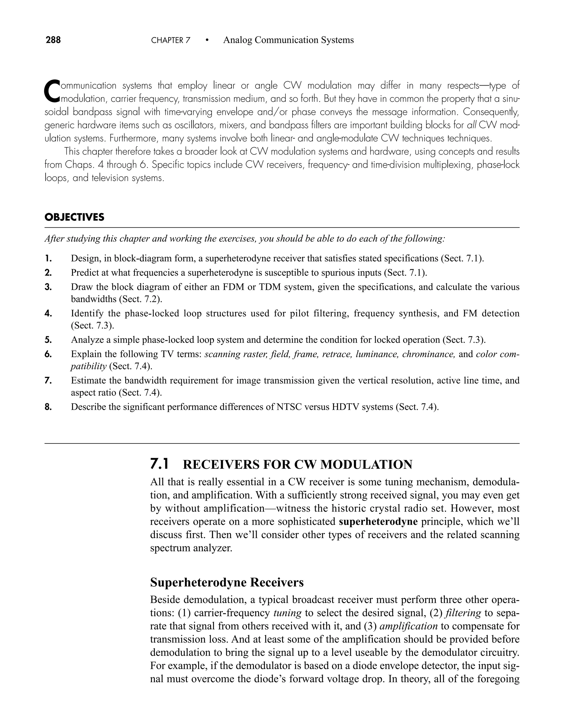
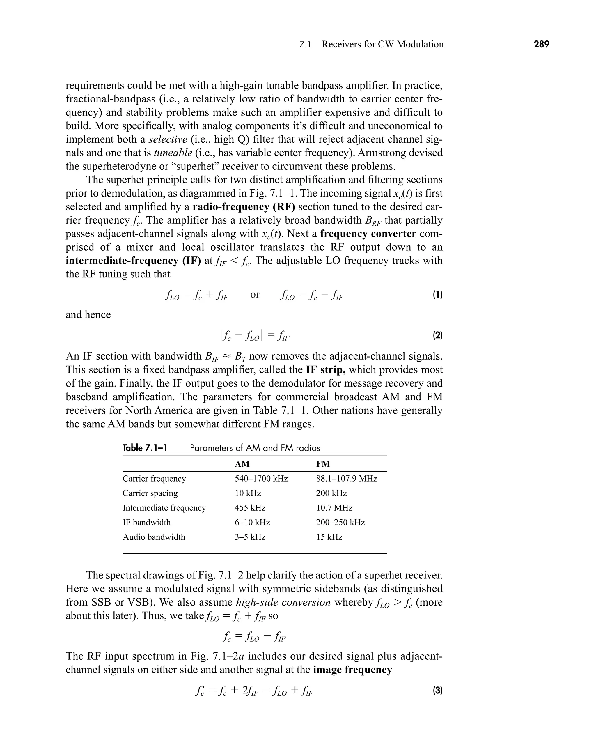
![xc(t)
x(t)
fc fIF
BIF ≈ BT
BT BRF 2fIF
fLO = fc ± fIF
RF IF
Other
signals
Antenna
LO
Mixer
Demod
Baseband
×
Figure 7.1–1 Superheterodyne receiver.
(a)
(b)
RF
input
IF
input
f
f
|HRF( f )| fLO
fc = fLO – fIF fc′ = fLO + fIF
BRF
fIF
BIF
BT
|HIF( f )|
Figure 7.1–2 Spectrums in a superhetrodyne receiver. (a) At the antenna, (b) in the IF section.
290 CHAPTER 7 • Analog Communication Systems
Note the two acceptable frequencies fc and are a consequence of the absolute value
operator of Eq. (2).†
The main task of the RF section is to pass at least fc BT/2 while rejecting the
image frequency signal. For to reach the mixer, it would be down-converted to
and the image frequency signal would produce an effect similar to cochannel inter-
ference. Hence, we want an RF response HRF(f ) like the dashed line, with
(4)
Note also, as indicated in Fig 7.1–2, fLO has to be outside the tunable front-end BPF
to avoid blocking effects.You can also observe that, the higher the IF, the greater will
be the image frequency, thus reducing the need for a narrowband BPF for the front
BT 6 BRF 6 2fIF
f ¿
c fLO 1 fLO fIF 2 fLO fIF
f œ
c
f œ
c
†
Note also in the mixer stage
cosa cosb cosb cosa [cos(a b) cos(a b)] [cos(b a) cos(b a)]
1
2
1
2
car80407_ch07_287-344.qxd 12/16/08 6:10 PM Page 290](https://image.slidesharecdn.com/communicationsystemsanintro-a-241115060943-61721fa8/75/Communication_Systems__An_Intro_-_A-_Bruce_Carlson_-pdf-312-2048.jpg)
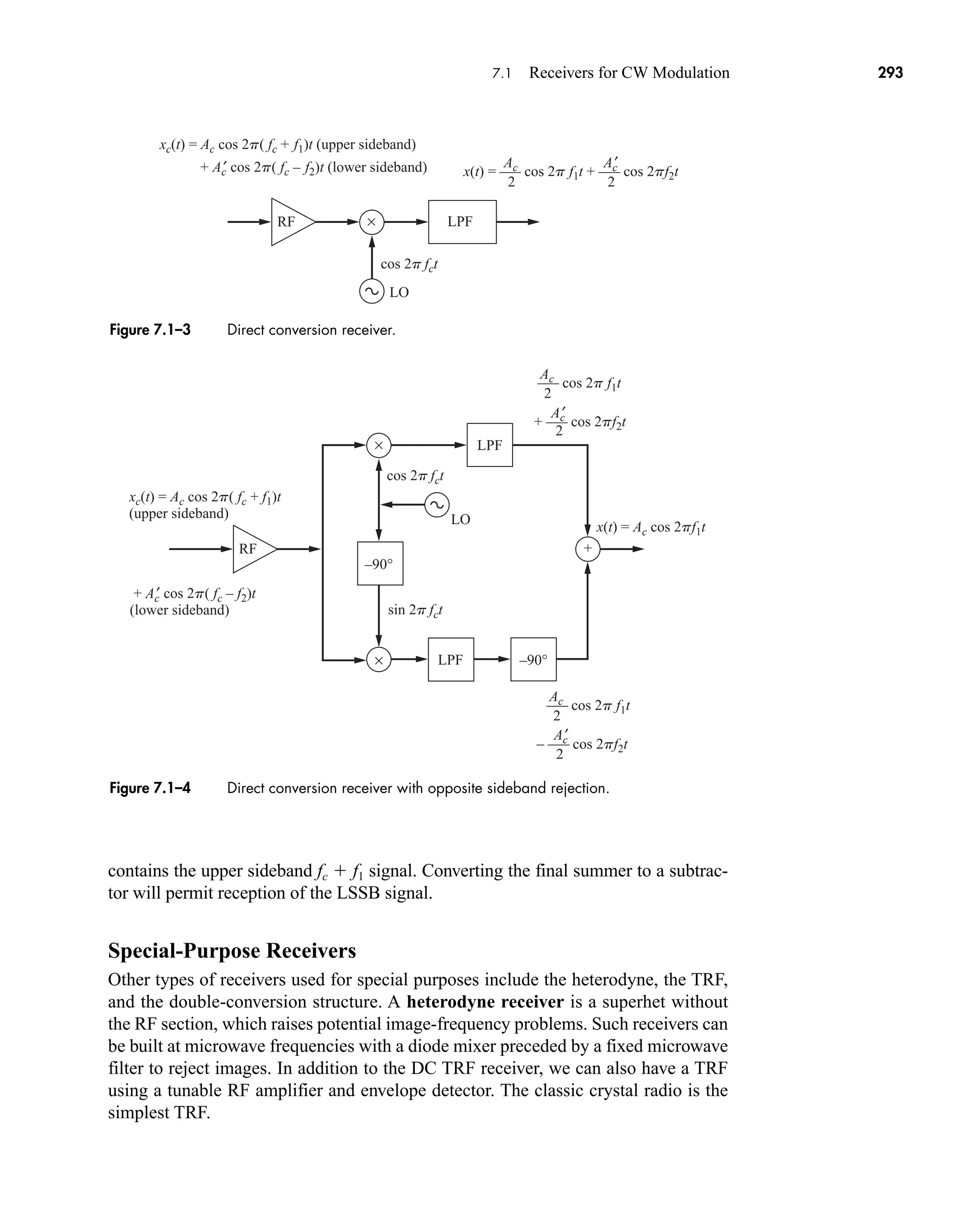
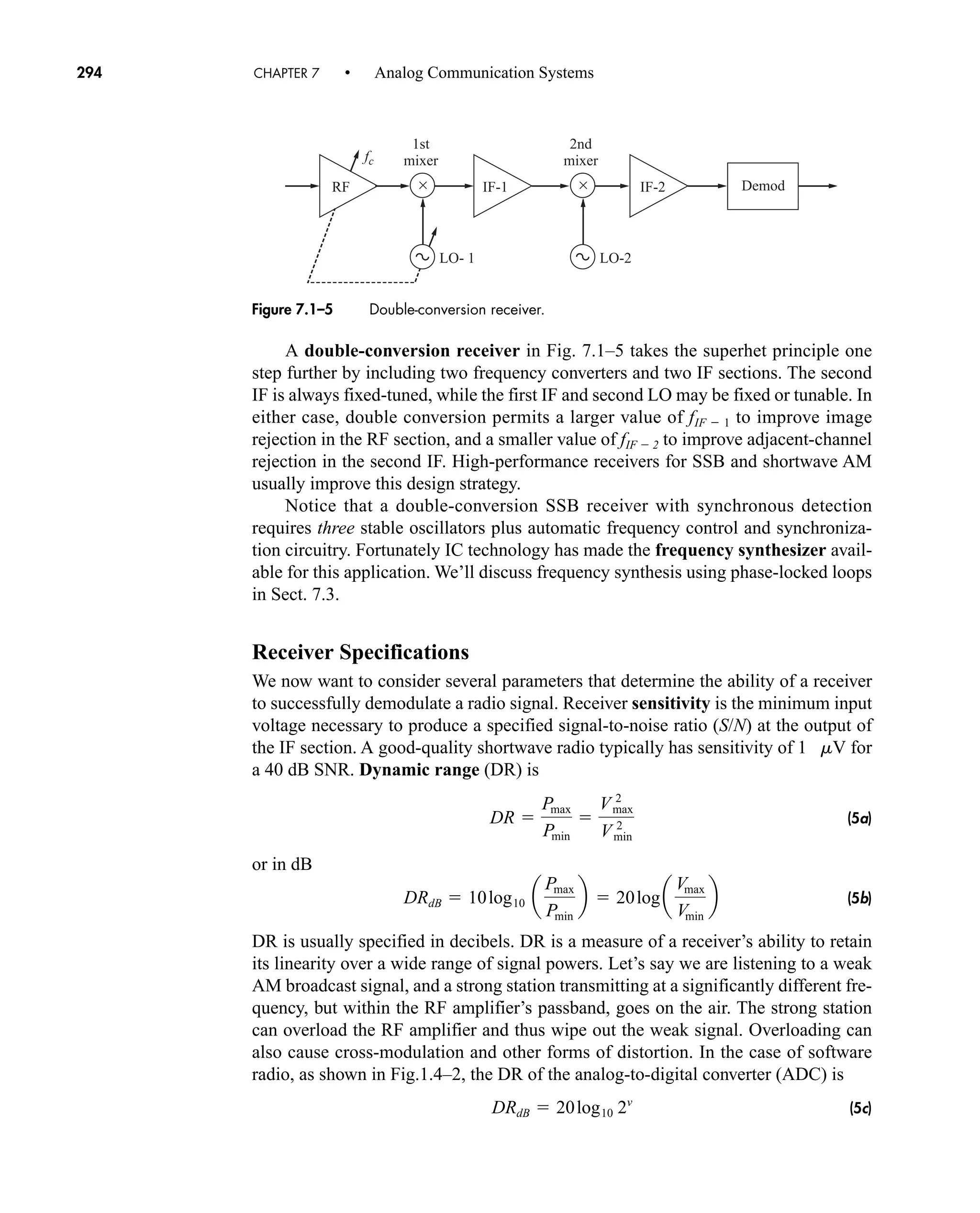
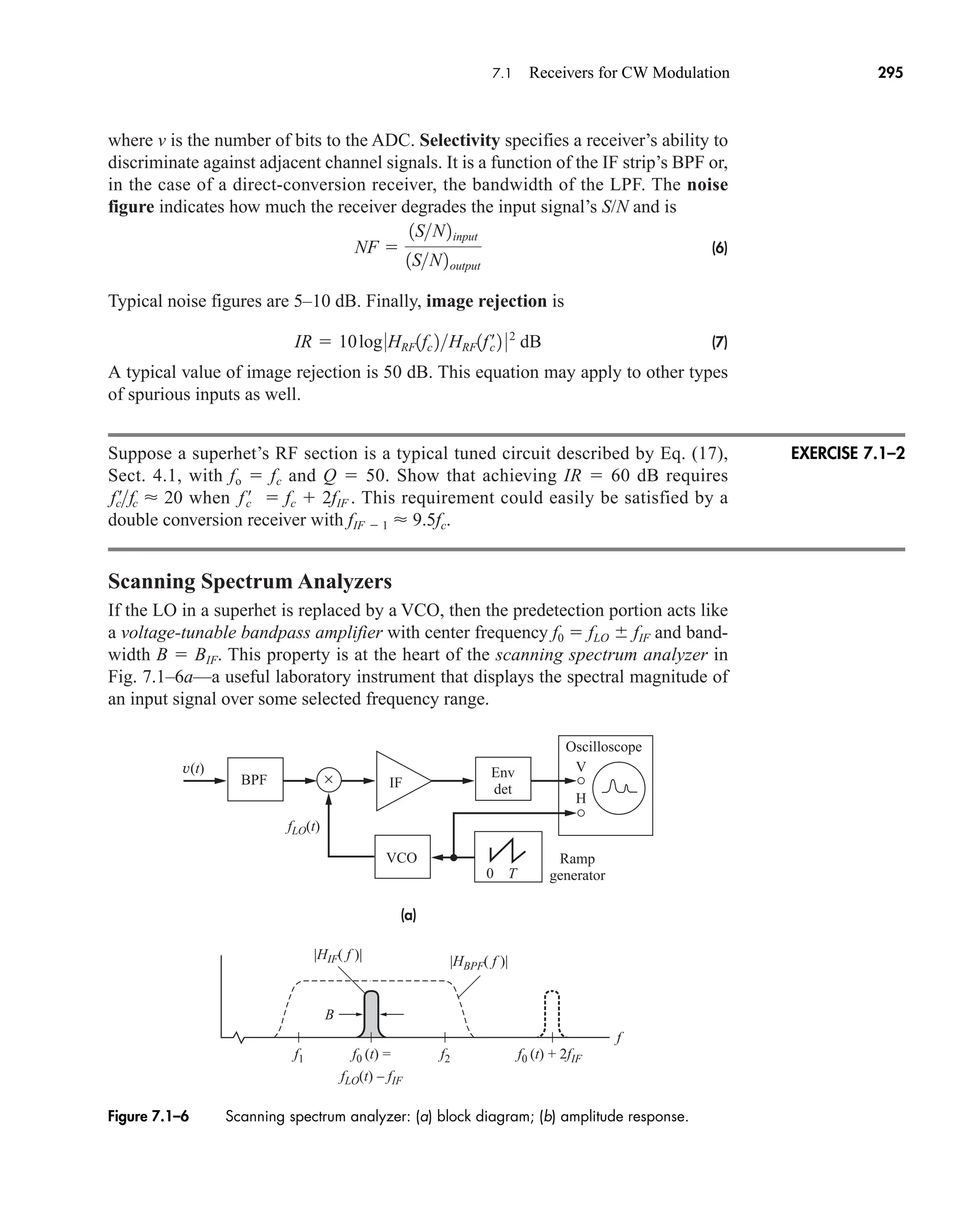
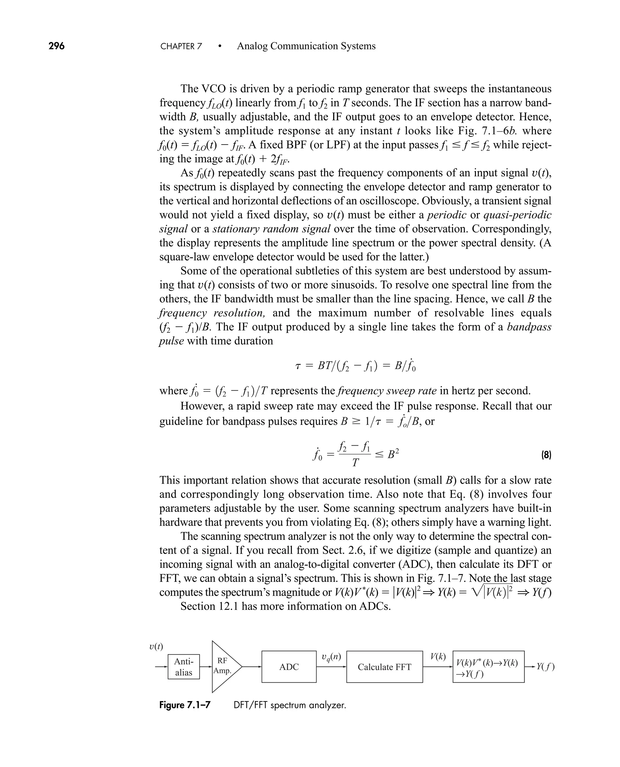
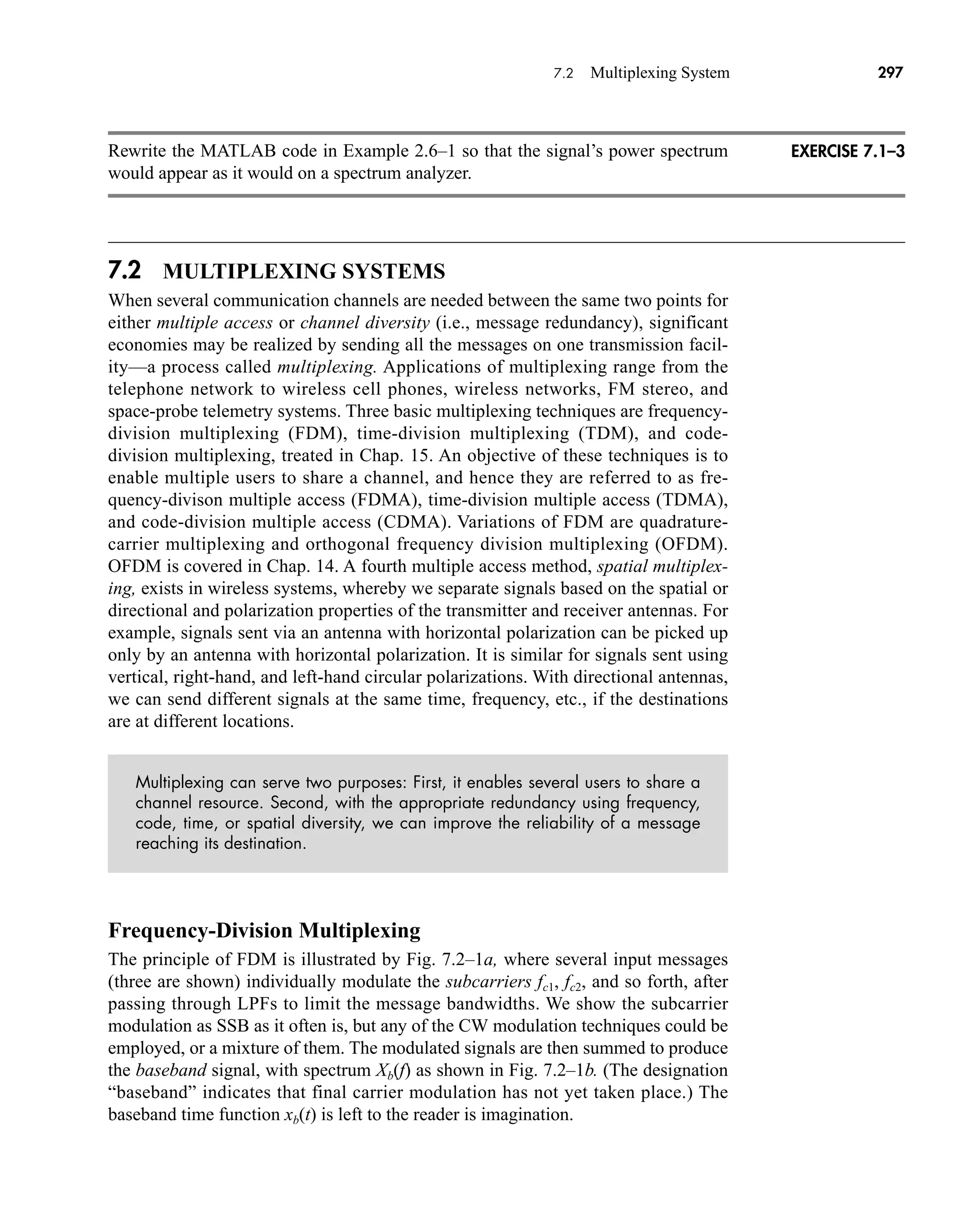
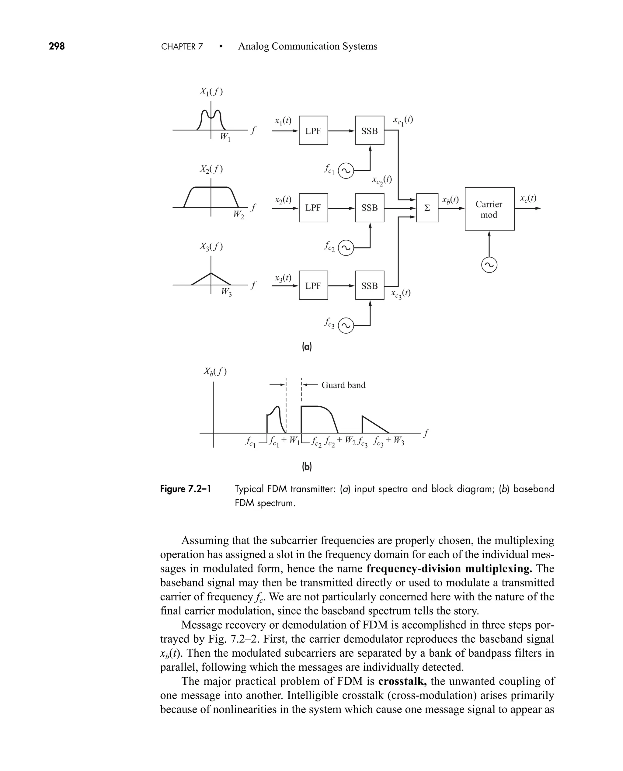
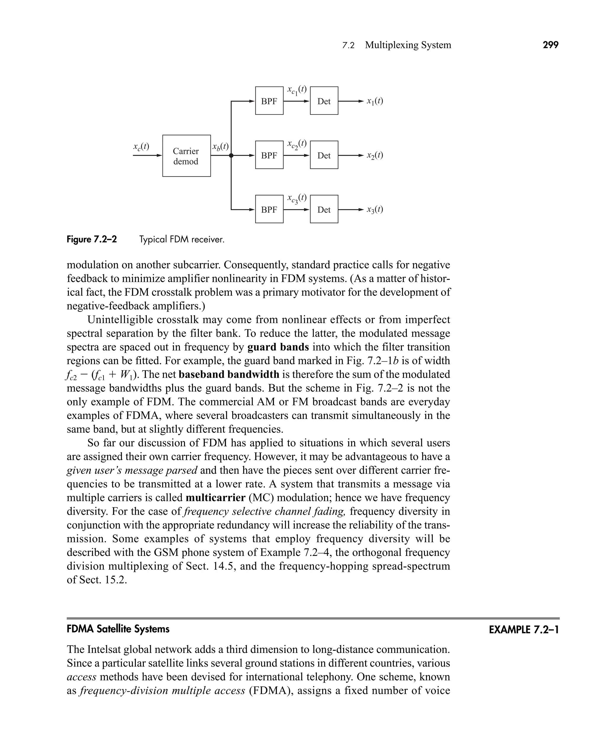
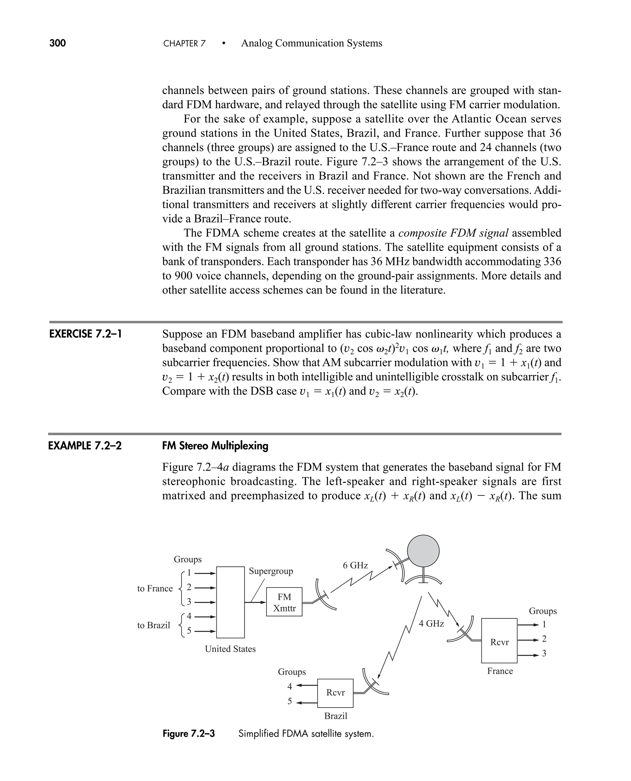
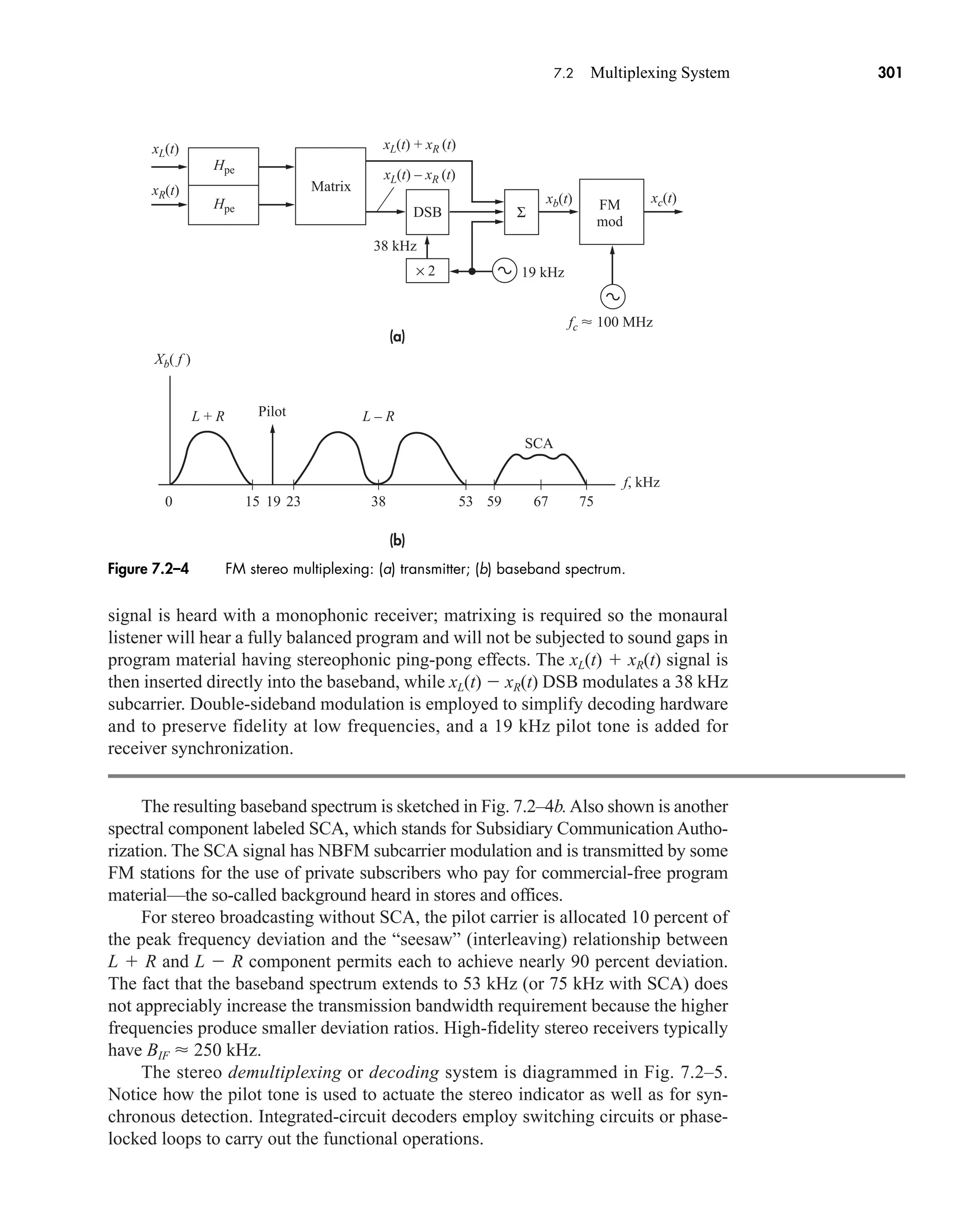
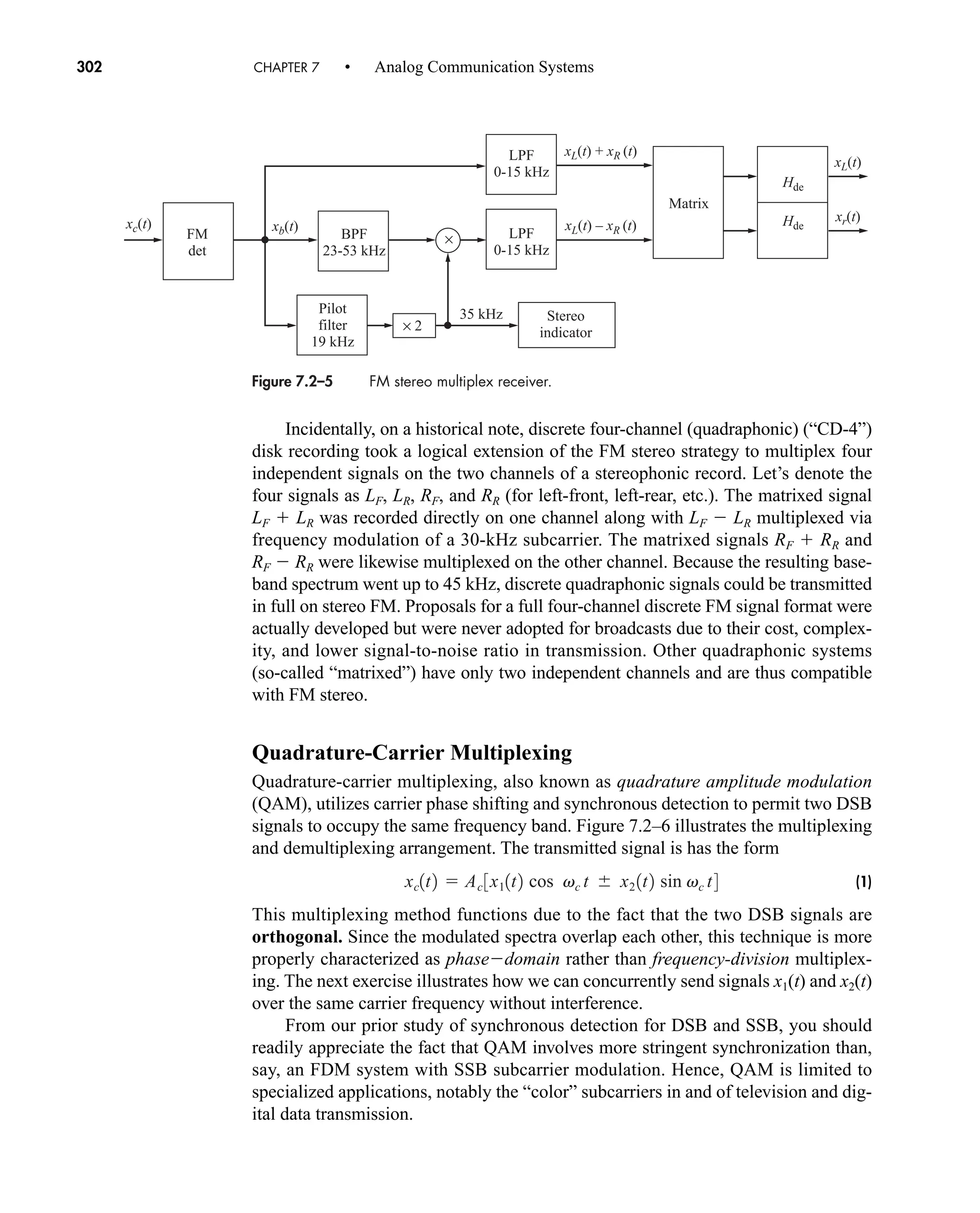
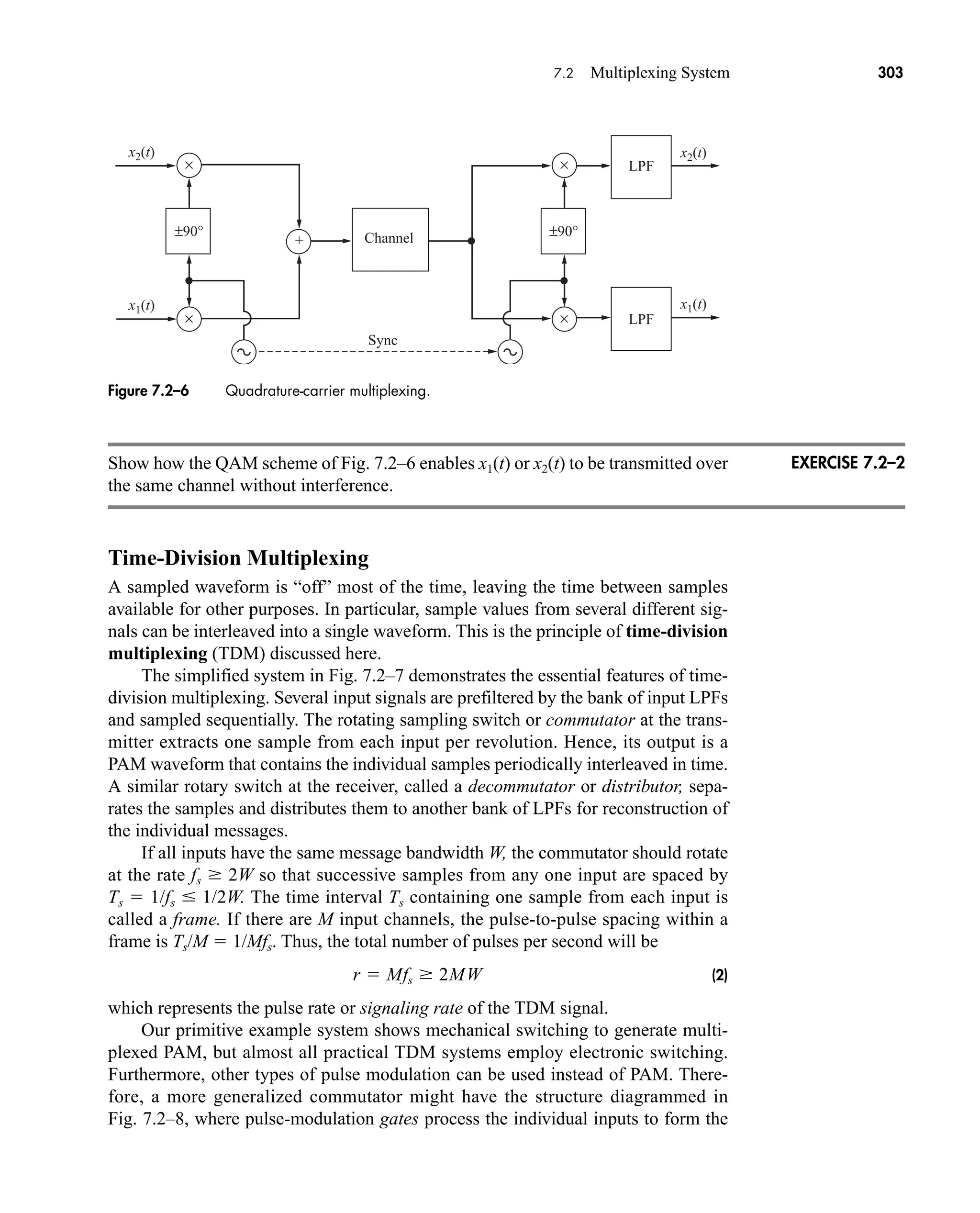
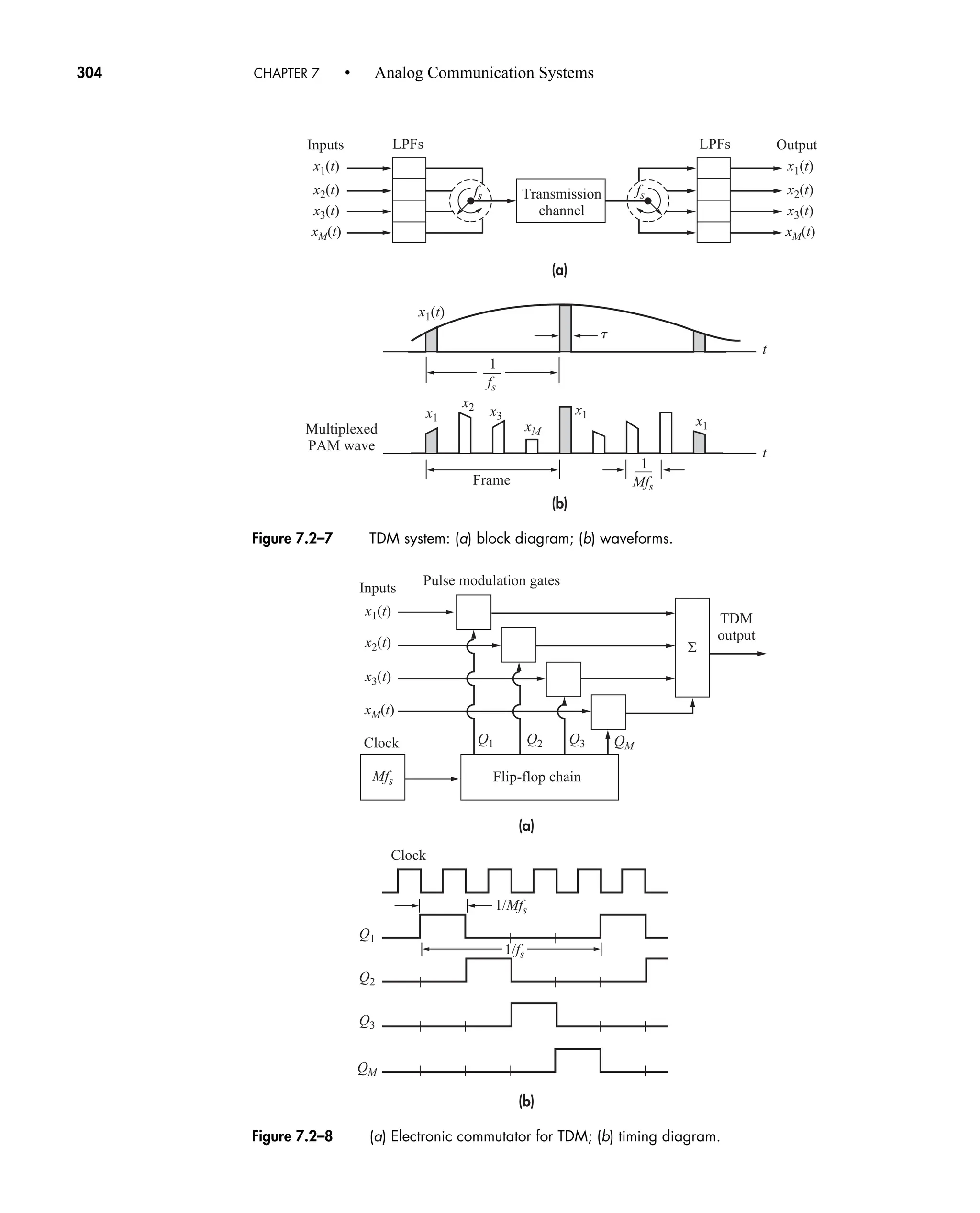
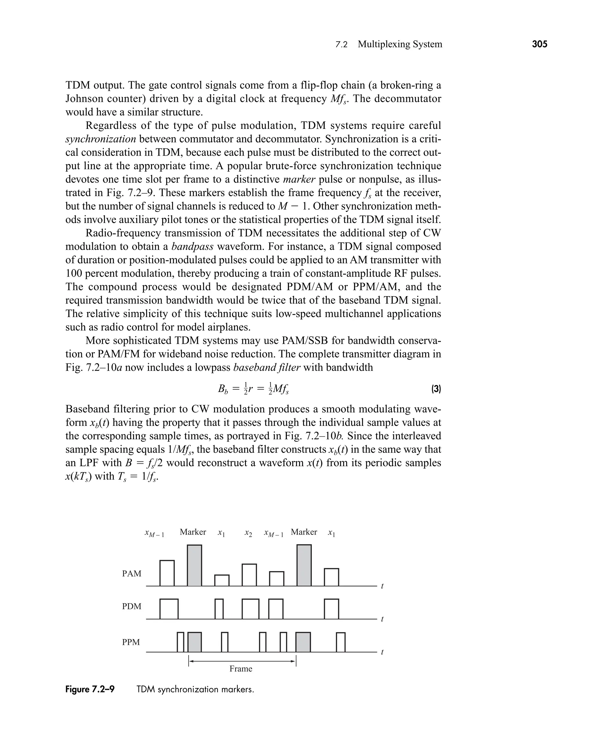
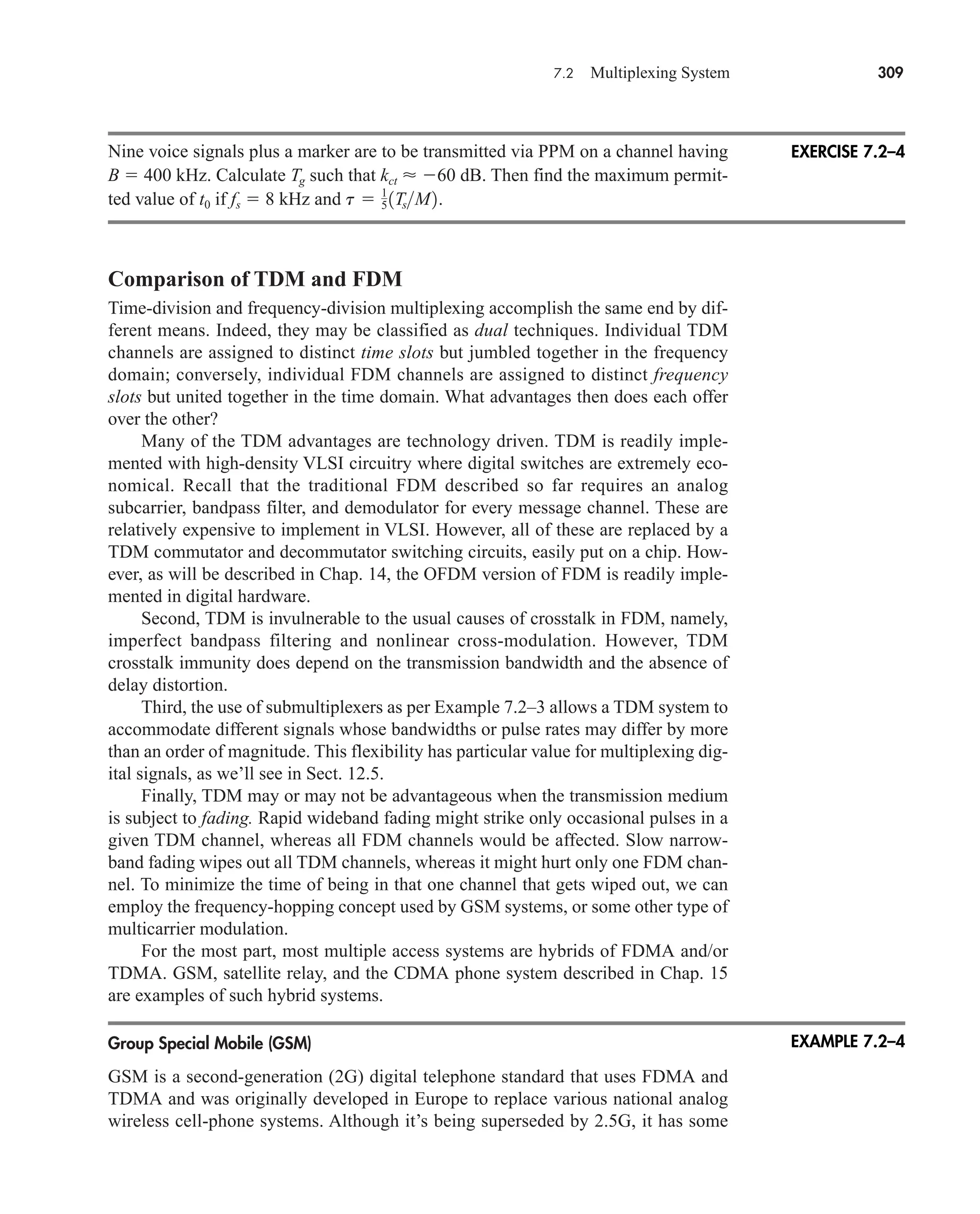
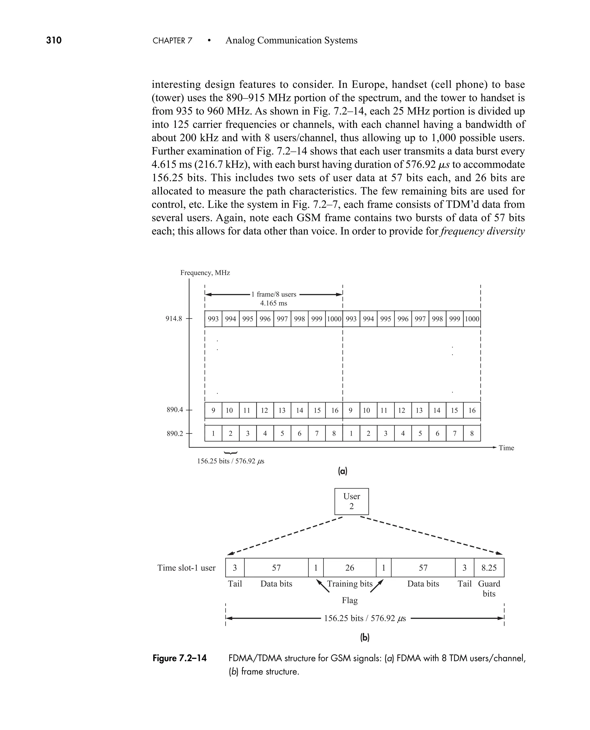
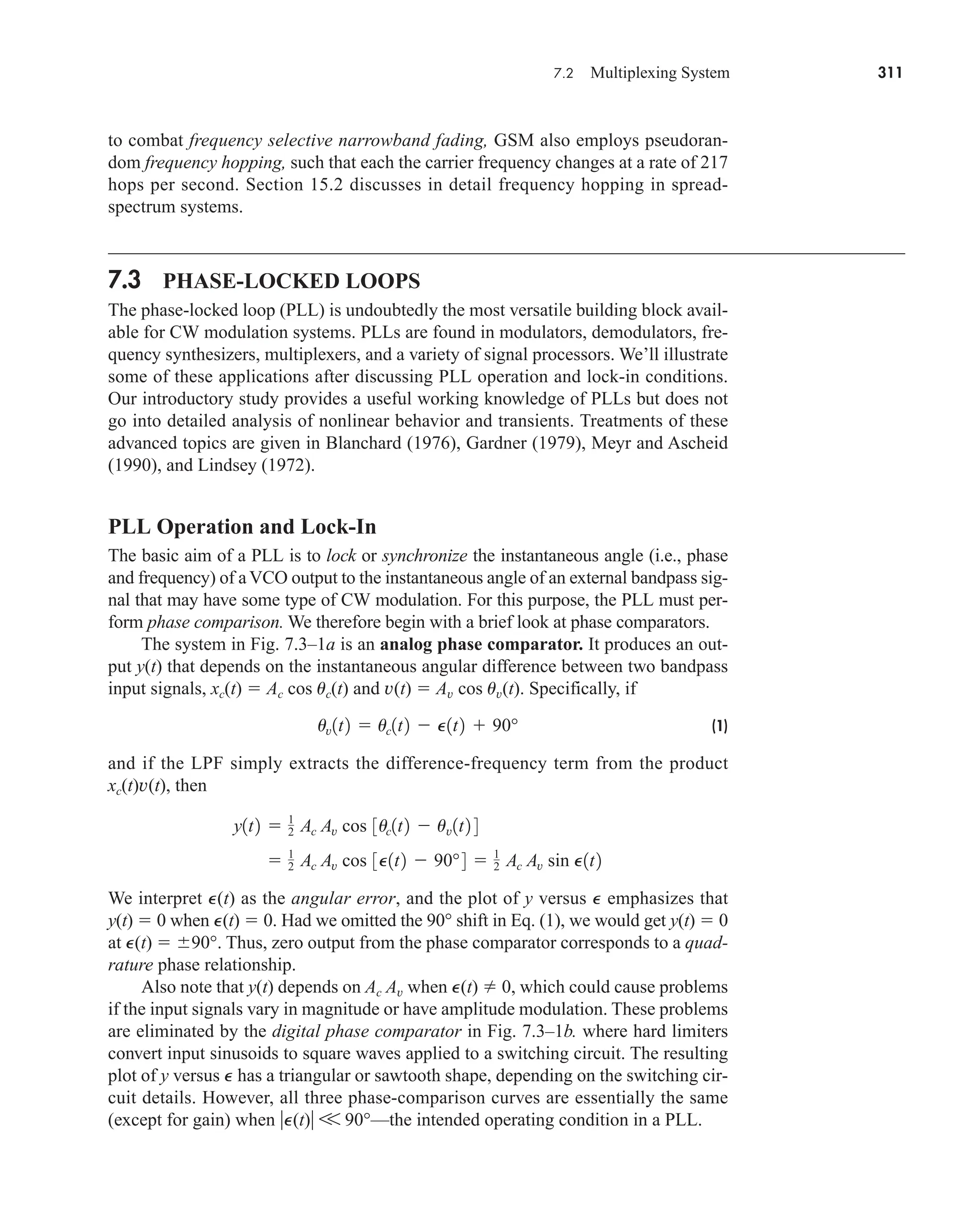
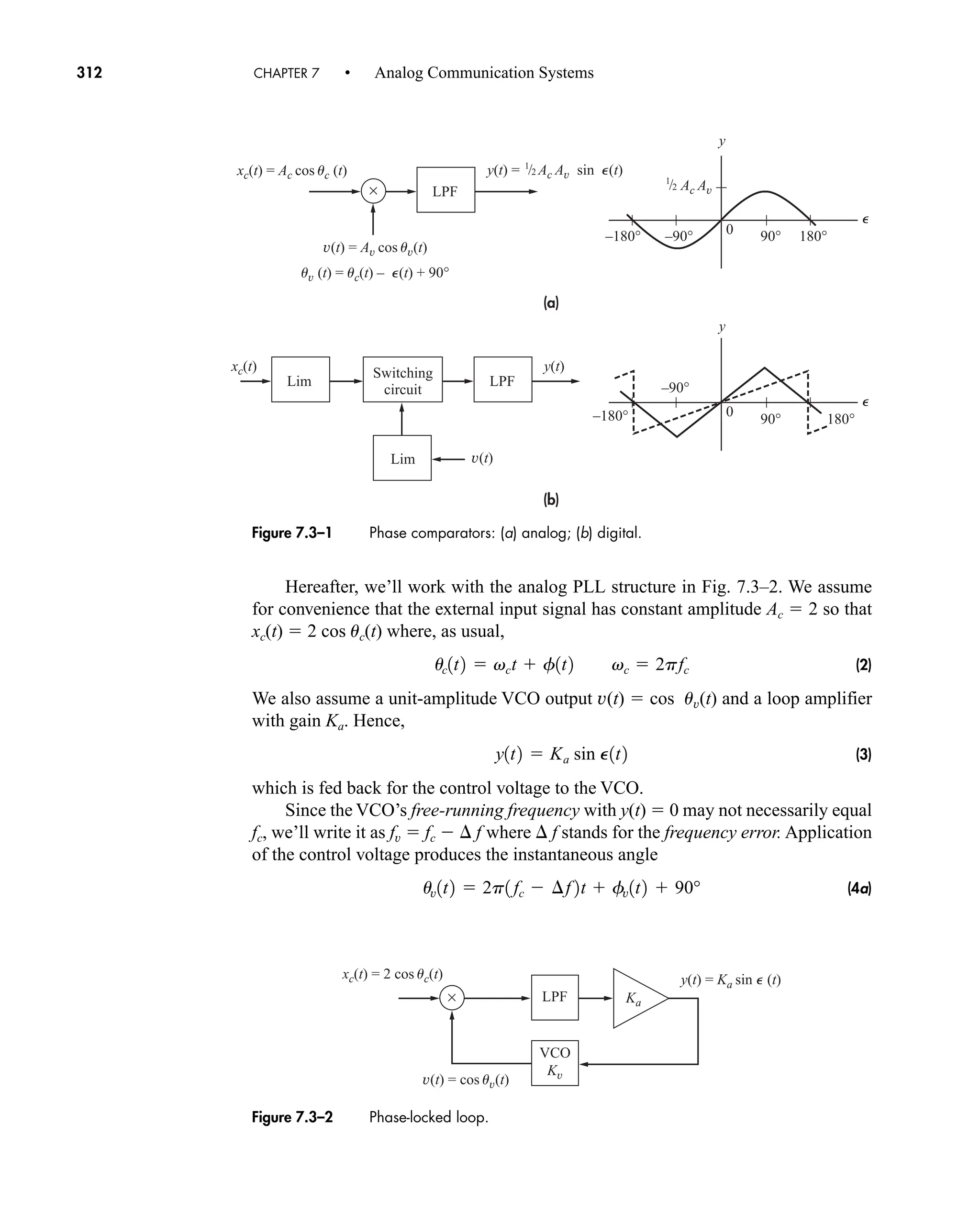
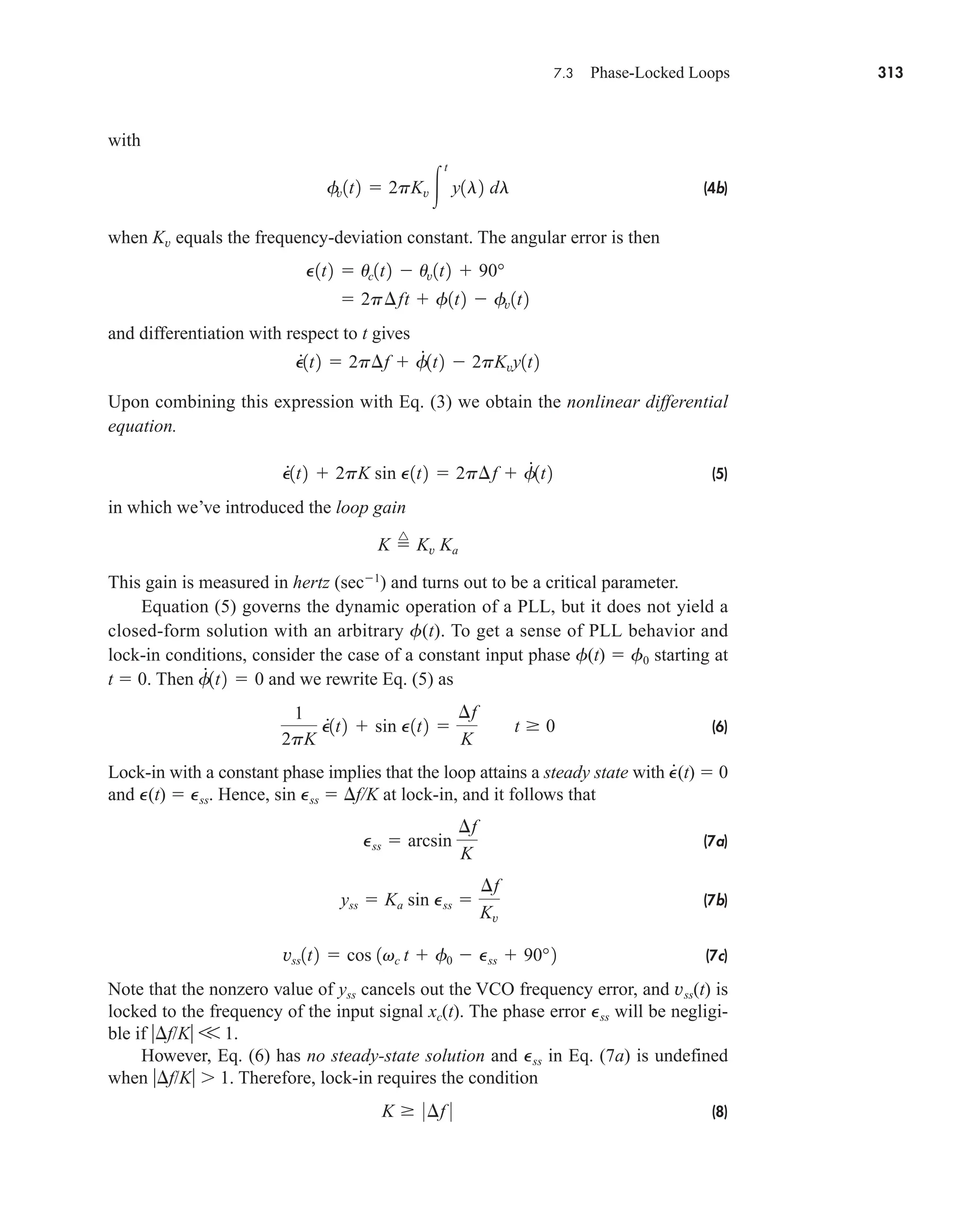
![×
–90°
t
t – T
∫
Main PD
VCO
2
T
Multiplier
(error signals)
Quad PD
x(t) cos Pss
x(t) cos vct
cos (vct – Pss + 90°)
x(t) sin Pss
yss ≈ –– Sx sin 2 Pss
Output
Figure 7.3–4 Costas PLL system for synchronous detection.
7.3 Phase-Locked Loops 315
used to generate a sinusoid synchronized with the pilot. To minimize clutter here,
we’ve lumped the phase comparator, lowpass filter, and amplifier into a phase dis-
criminator (PD) and we’ve assumed unity sinusoidal amplitudes throughout.
Initial adjustment of the tuning voltage brings the VCO frequency close to fc and
Pss 0, a condition sensed by the quadrature phase discriminator and displayed by
the lock-in indicator. Thereafter, the PLL automatically tracks any phase or fre-
quency drift in the pilot, and the phase-shifted VCO output provides the LO signal
needed for the synchronous detector. Thus, the whole unit acts as a narrowband pilot
filter with a virtually noiseless output.
Incidentally, a setup like Fig. 7.3–3 can be used to search for a signal at some
unknown frequency. You disconnect the VCO control voltage and apply a ramp gen-
erator to sweep the VCO frequency until the lock-in indicator shows that a signal has
been found. Some radio scanners employ an automated version of this procedure.
For synchronous detection of DSB without a transmitted pilot, Costas invented
the PLL system in Fig. 7.3–4. The modulated DSB waveform x(t) cos vct with band-
width 2W is applied to a pair of phase discriminators whose outputs are proportional
to x(t) sin Pss and x(t) cos Pss. Multiplication and integration over T W 1/W produces
the VCO control voltage
If f 0, the PLL locks with Pss 0 and the output of the quadrature discriminator
is proportional to the demodulated message x(t). Of course the loop loses lock if
x(t) 0 for an extended interval.
The frequency-offset loop in Fig. 7.3–5 translates the input frequency (and
phase) by an amount equal to that of an auxiliary oscillator. The intended output fre-
quency is now fc f1, so the free-running frequency of the VCO must be
The oscillator and VCO outputs are mixed and filtered to obtain the difference-
frequency signal cos [uv(t) (v1t f1)] applied to the phase discriminator. Under
locked conditions with Pss 0, the instantaneous angles at the input to the
discriminator will differ by 90. Hence, uv(t) (v1t f1) vct f0 90, and
the VCO produces cos [(vc v1)t f0 f1 90].
fv 1 fc f1 2 ¢f fc f1
yss T8x2
1t2 9 sin Pss cos Pss
T
2
Sx sin 2Pss
car80407_ch07_287-344.qxd 12/16/08 6:10 PM Page 315](https://image.slidesharecdn.com/communicationsystemsanintro-a-241115060943-61721fa8/75/Communication_Systems__An_Intro_-_A-_Bruce_Carlson_-pdf-337-2048.jpg)
![fv ≈ nfc
÷ n
VCO
PD
cos (nvct + nf0 + n90°)
cos (vct + f0)
cos [uv(t)/n]
Figure 7.3–6 PLL frequency multiplier.
cos uv(t)
cos [(vc + v1)t + f0 + f1 + 90°]
fv ≈ fc + f1
cos (vct + f0)
cos (v1t + f1)
PD
LPF
Mixer
Aux. osc.
VCO
Figure 7.3–5 Frequency-offset loop.
316 CHAPTER 7 • Analog Communication Systems
By likewise equating instantaneous angles, you can confirm that Fig. 7.3–6 per-
forms frequency multiplication. Like the frequency multiplier discussed in Sect. 5.2,
this unit multiplies the instantaneous angle of the input by a factor of n. However, it
does so with the help of a frequency divider which is easily implemented using a
digital counter. Commercially available divide-by-n counters allow you to select any
integer value for n from 1 to 10 or even higher. When such a counter is inserted in a
PLL, you have an adjustable frequency multiplier.
A frequency synthesizer starts with the output of one crystal-controlled master
oscillator; various other frequencies are synthesized therefrom by combinations of
frequency division, multiplication, and translation. Thus, all resulting frequencies
are stabilized by and synchronized with the master oscillator. General-purpose labo-
ratory synthesizers incorporate additional refinements and have rather complicated
diagrams, so we’ll illustrate the principles of frequency synthesis by an example.
Adjustable Local Oscillator Using a Frequency Synthesizer
Suppose a double-conversion SSB receiver needs fixed LO frequencies at 100 kHz
(for synchronous detection) and 1.6 MHz (for the second mixer), and an adjustable
LO that covers 9.90–9.99 MHz in steps of 0.01 MHz (for RF tuning). The custom-
tailored synthesizer in Fig. 7.3–7 provides all the required frequencies by dividing
down, multiplying up, and mixing with the output of a 10 MHz oscillator. You can
quickly check out the system by putting a frequency-multiplication block in place of
each PLL with a divider.
EXAMPLE 7.3–1
car80407_ch07_287-344.qxd 12/11/08 11:03 PM Page 316](https://image.slidesharecdn.com/communicationsystemsanintro-a-241115060943-61721fa8/75/Communication_Systems__An_Intro_-_A-_Bruce_Carlson_-pdf-338-2048.jpg)

![+
–
+
–
(a)
× h(t)
y(t)
v(t) = cos [vct + fv(t) + 90°]
f(t)
Φ( f )
Φv( f )
xc(t) = 2 cos [vct + f(t)]
Ka
t
∫
VCO
(b)
+ h(t) y(t)
Ka
2pKv
(c)
+ H( f ) Y( f )
Ka
Kv/jf
fv(t)
Figure 7.3–8 Linearized PLL models: (a) time domain; (b) phase; (c) frequency domain.
318 CHAPTER 7 • Analog Communication Systems
Fourier transformation finally takes us to the frequency-domain model in
Fig. 7.3–8c. where and so forth. Routine analysis
yields
(10)
which expresses the frequency-domain relationship between the input phase and out-
put voltage.
Now let xc(t) be an FM wave with and, accordingly,
Substituting for (f) in Eq. (10) gives
(11a)
where
(11b)
HL1 f 2
H1 f 2
H1 f 2 j1 fK2
Y1 f 2
f¢
Kv
HL1 f 2X1 f 2
£1 f 2 2pf¢ X1 f 21 j2pf 2 1 f¢jf 2X1 f 2
f
#
1t2 2pf¢ x1t2
Y1 f 2
Ka H1 f 2
1 Ka H1 f 21Kvjf 2
£1 f 2
1
Kv
jfKH1 f 2
jf KH1 f 2
£1 f 2
£1f2 3f1t2 4, H1f2 3h1t2 4,
car80407_ch07_287-344.qxd 12/16/08 6:10 PM Page 318](https://image.slidesharecdn.com/communicationsystemsanintro-a-241115060943-61721fa8/75/Communication_Systems__An_Intro_-_A-_Bruce_Carlson_-pdf-340-2048.jpg)
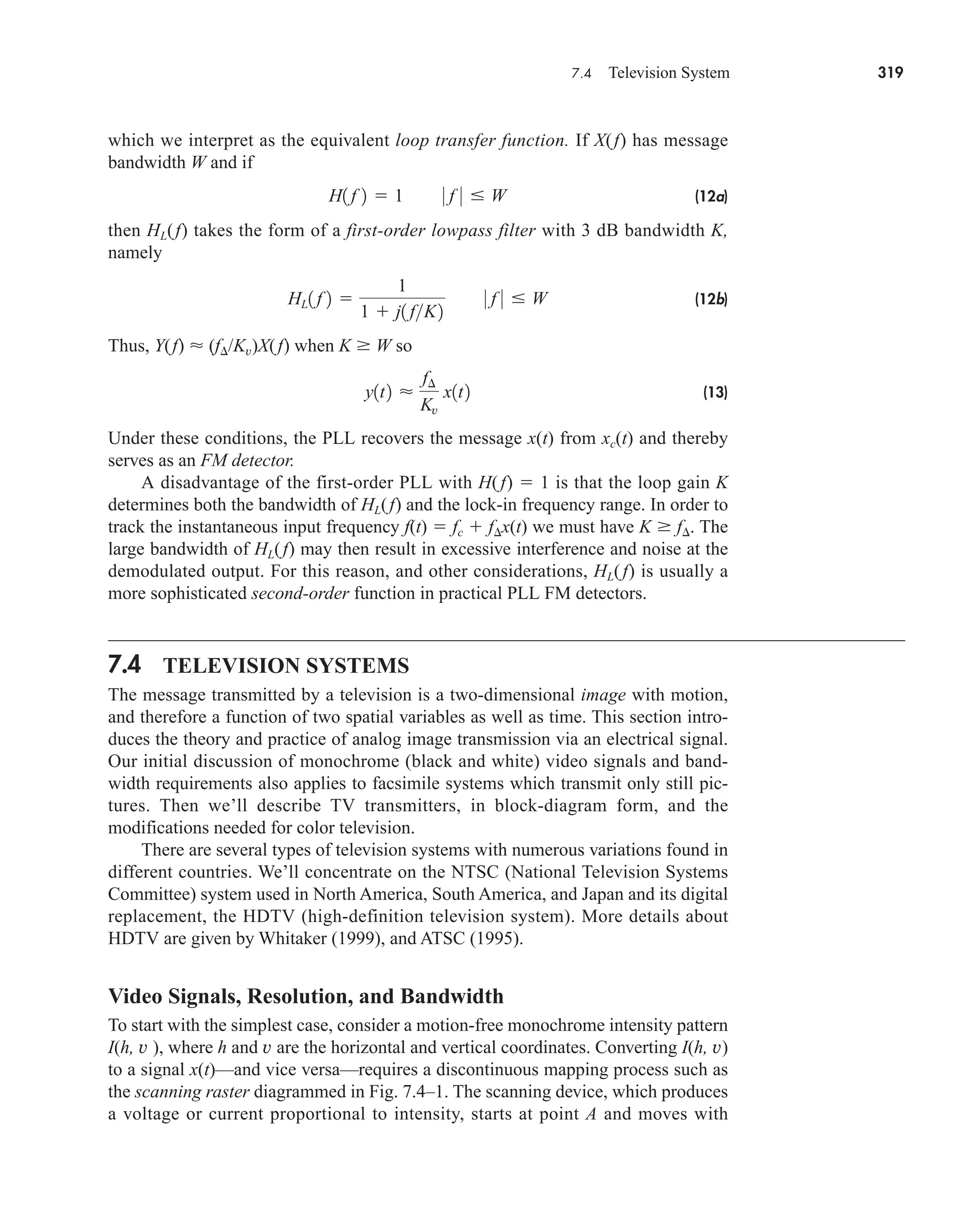
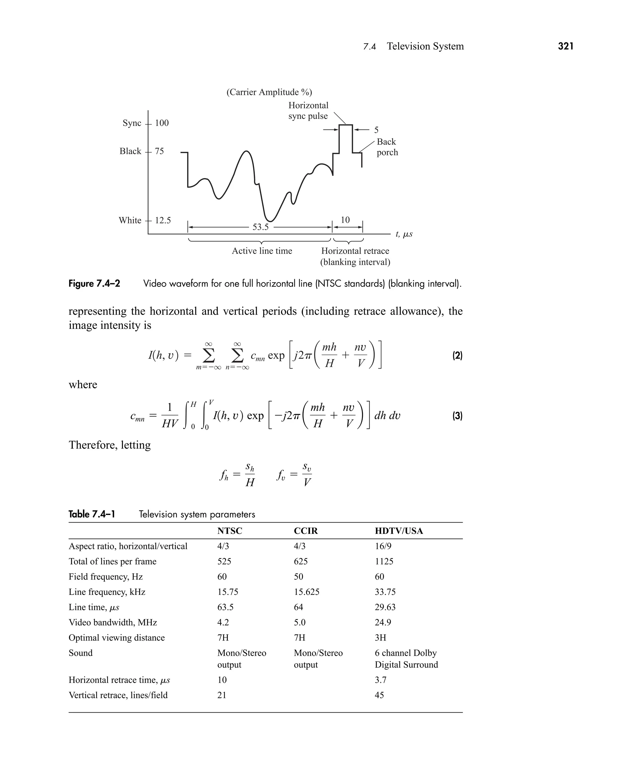
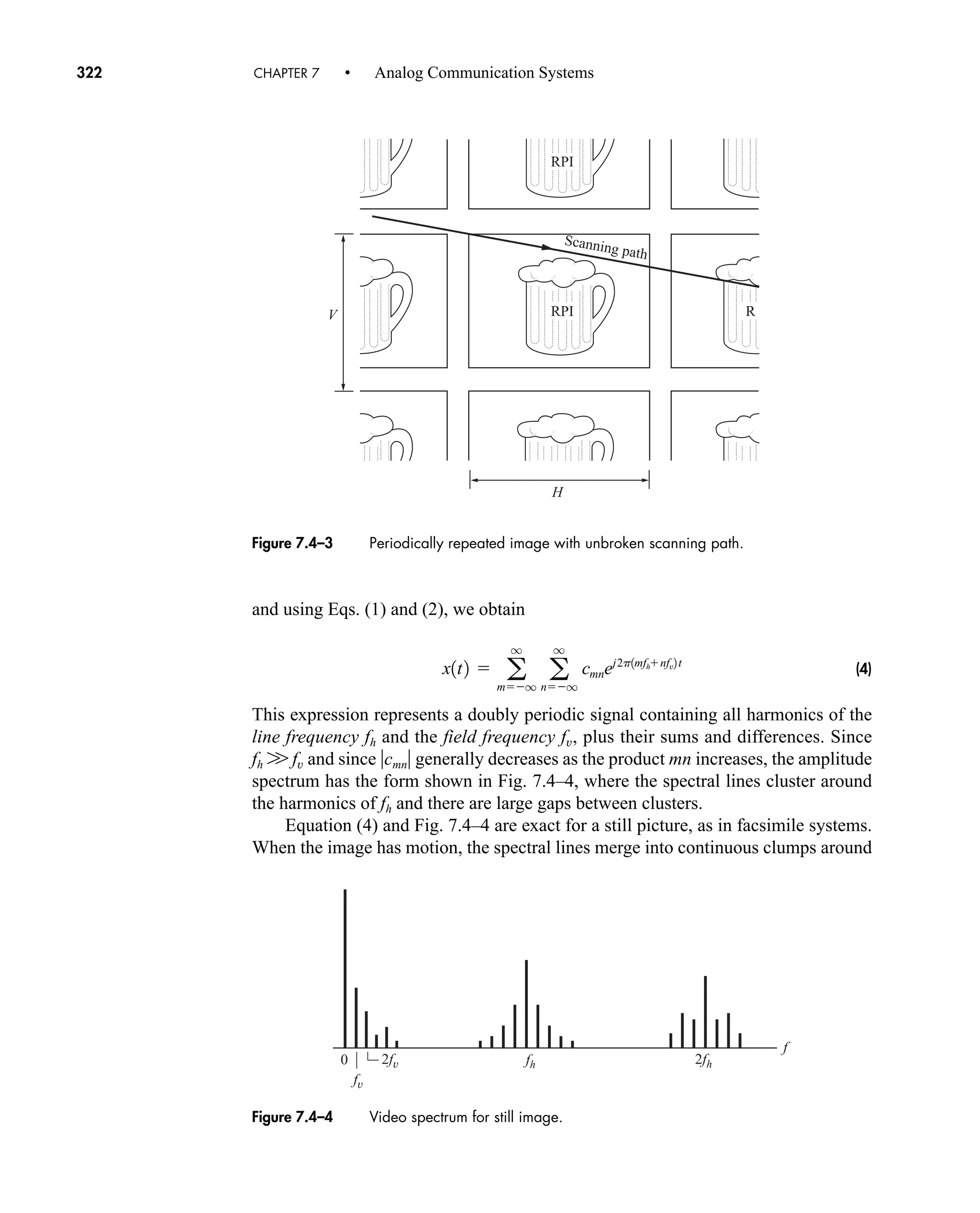
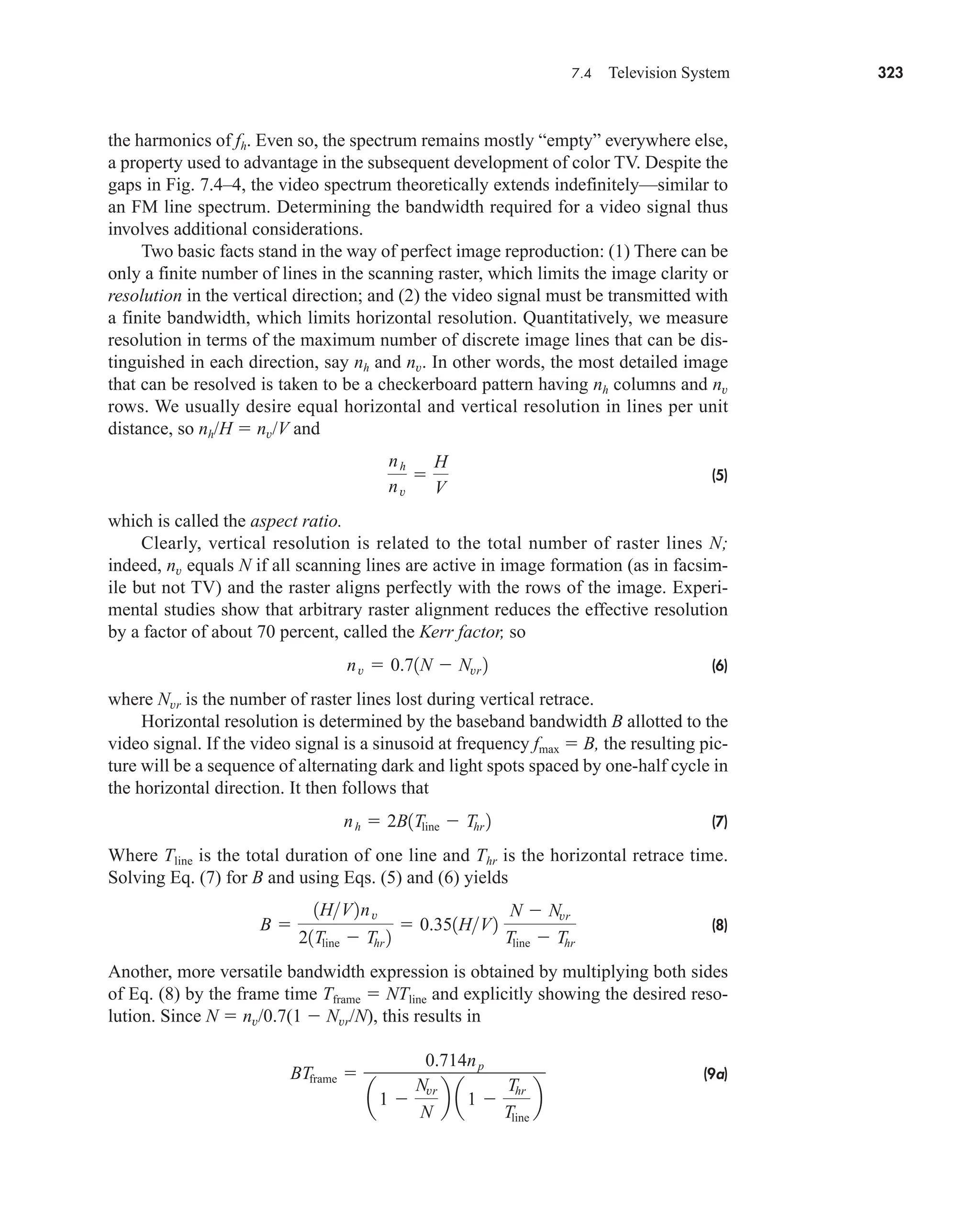
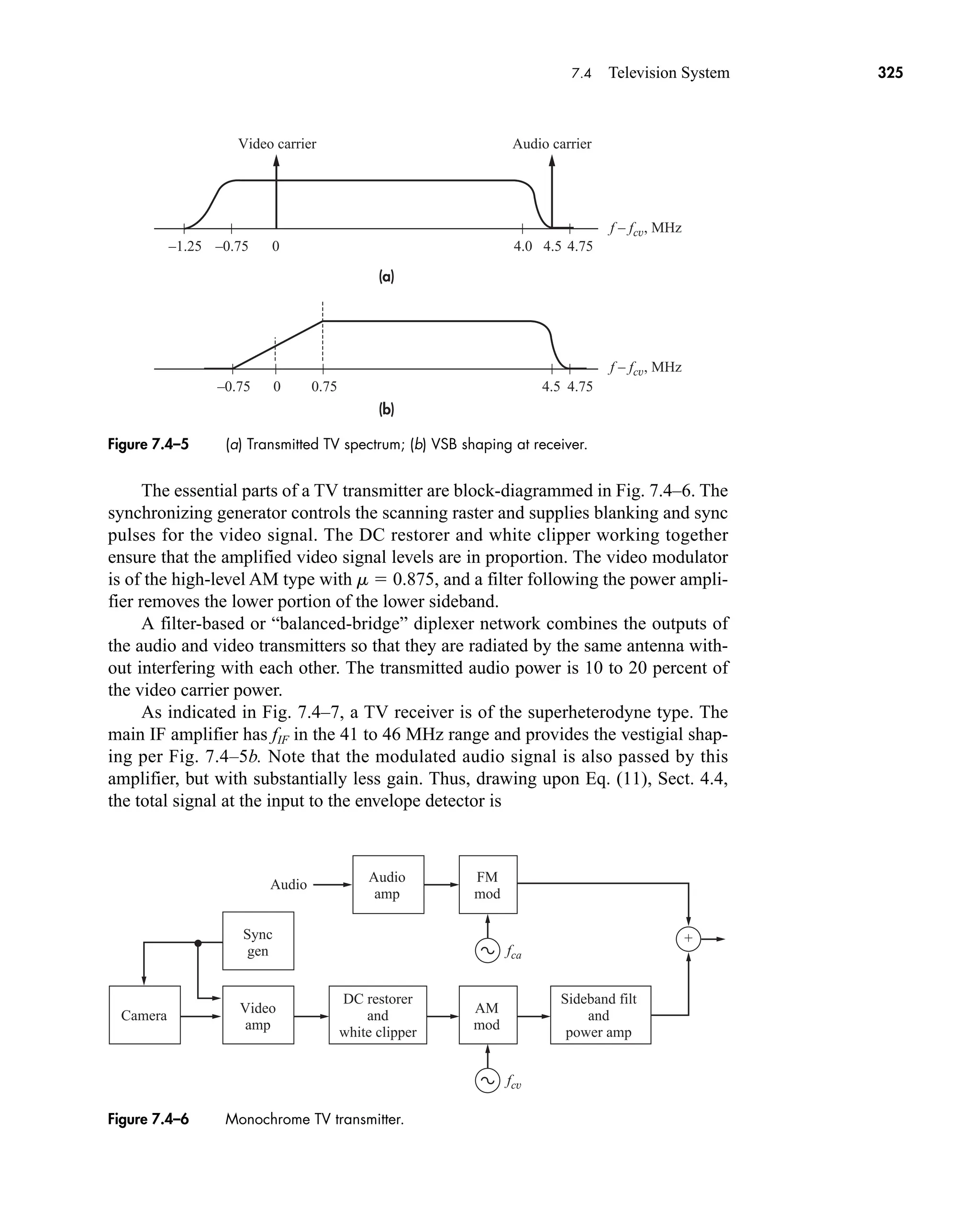
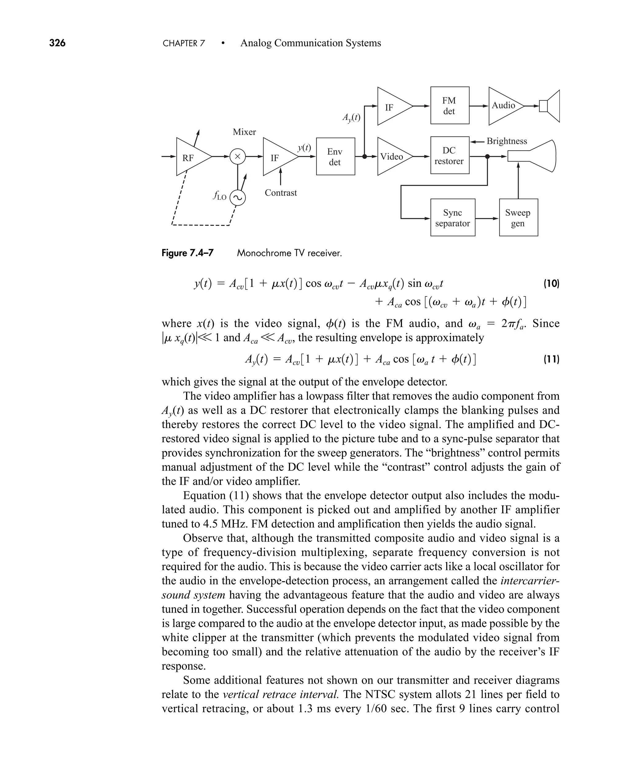
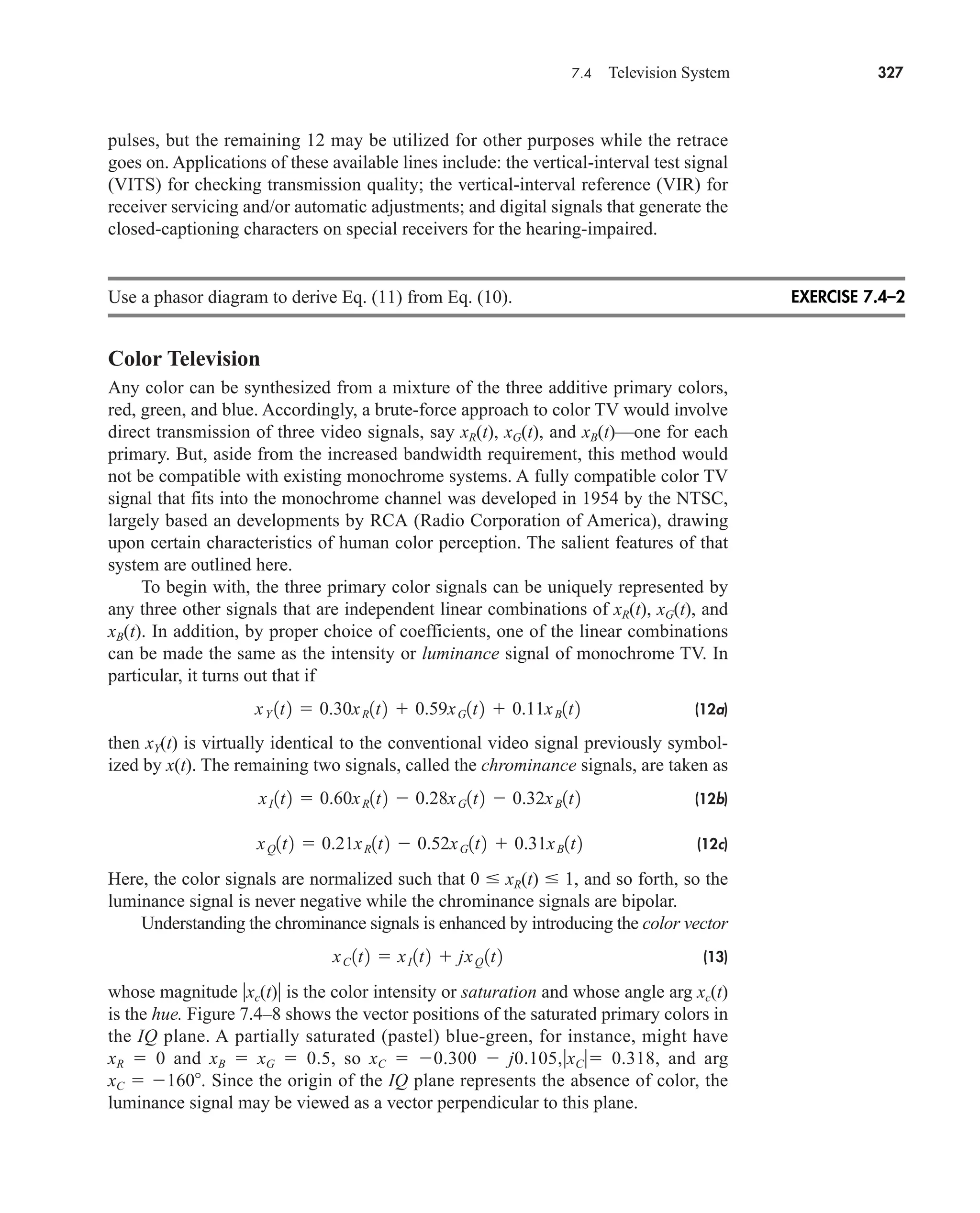
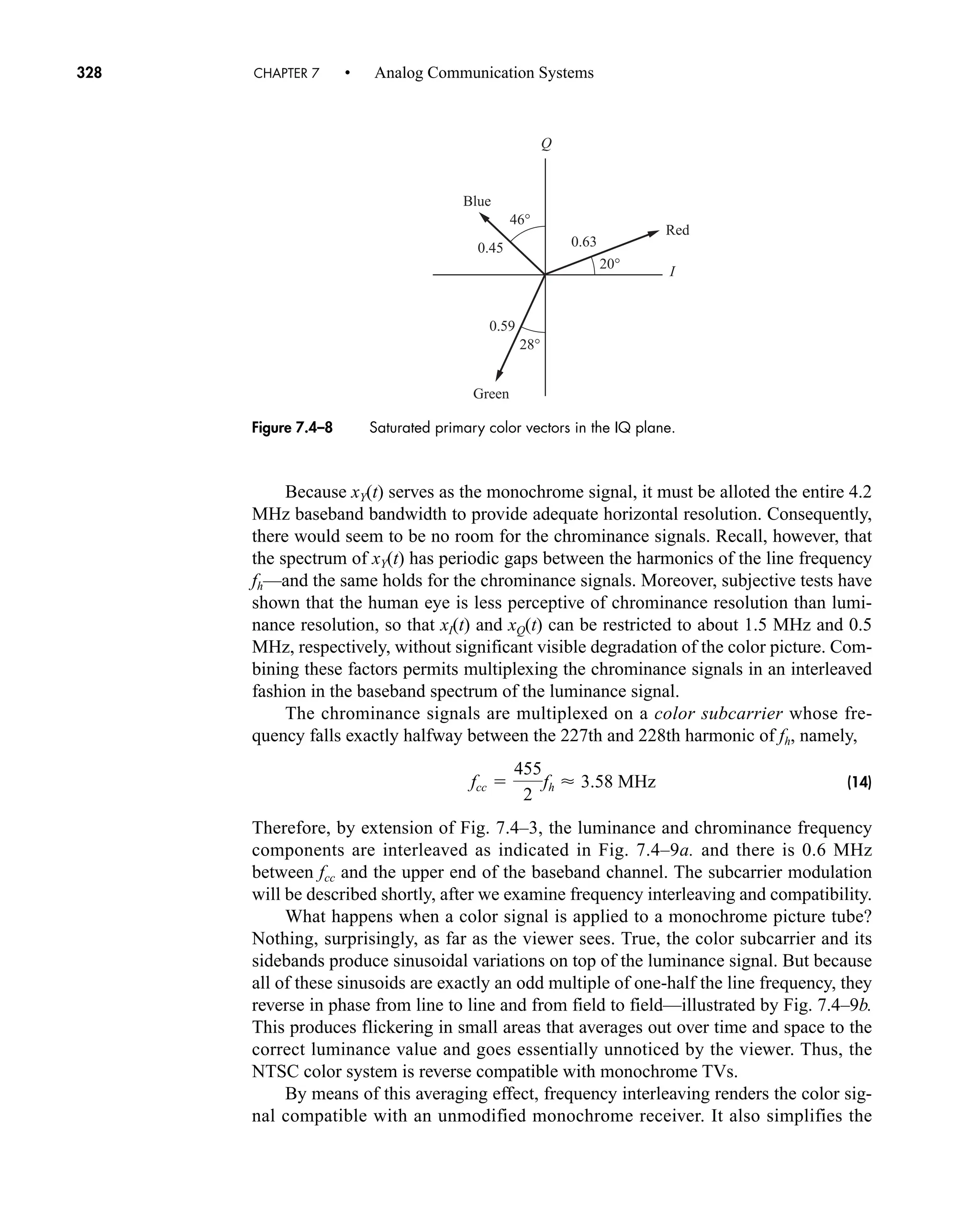
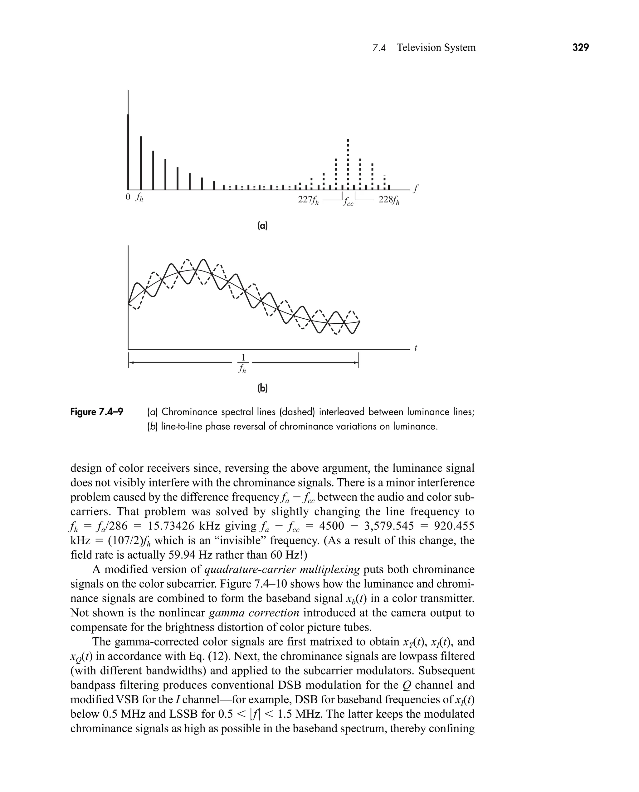
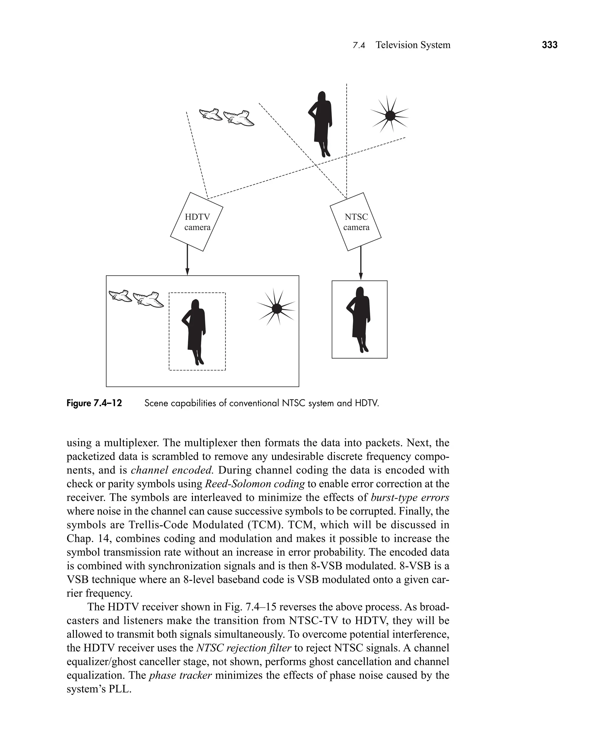
![338 CHAPTER 7 • Analog Communication Systems
7.1–7 Do Prob. 7.1–6 for LSSB modulation with W 6 kHz and
fc 7.14–7.26 MHz.
7.1–8 Sketch the spectrum of xc(t) cos 2p fLOt to demonstrate the sideband-
reversal effect in an SSB superhet when fLO fc fIF.
7.1–9 For automatic frequency control in an FM superhet, the LO is replaced
by a VCO that generates ALO cos u(t) with
.
u(t) 2p[fc fIF Kv(t)
P(t)] where P(t) is a slow and random frequency drift. The control volt-
age v(t) is derived by applying the demodulated signal to an LPF with
B V W. The demodulated signal is yD(t) where fIF(t) is
the instantaneous phase at the IF output. Analyze this AFC system by
finding yD(t) in terms of x(t) and P(t).
7.1–10* Consider a superhet that receives signals in the 50–54 MHz range with
fLO fc fIF. Assuming there is little filtering prior to the mixer, what
range of input signals will be received if the fIF is (a) 455 kHz, (b) 7
MHz?
7.1–11 Design a receiver that will receive USSB signals in the 50–54 MHz
range where fIF 100 MHz and does not exhibit sideband reversal.
Assume there is little filtering prior to the mixer. Specify fLO, the product
detector oscillator frequency, the center frequency of the IF bandpass
filter, and any image frequencies that will be received.
7.1–12 Consider a superhet with fLO fc fIF, fIF 455 kHz, and fc 2 MHz.
The RF amplifier is preceded by a first-order RLC bandpass filter with
f0 2 MHz and B 0.5 MHz. Assume the IF-BPF is nearly ideal and
that the mixer has unity gain. What is the minimum spurious frequency
input rejection ratio in dB?
7.1–13* Suppose the receiver in Prob. 7.1–12 has a LO with a second harmonic
whose voltage level is half that of the fundamental component. (a) What
input frequencies will be accepted, and at what power level in dB as
compared to the correct input? (b) Discuss all ways to minimize these
interfering inputs.
7.1–14 Consider a superhet that receives signals in the 7.0 to 8.0 MHz range
with fLO fc fIF, and fIF 455 kHz. The receiver’s RF amplifier has a
passband of 2 MHz, and its IF-BPF is nearly ideal and has a bandwidth
of 3 kHz. Design a frequency converter that has a fixed LO frequency
that will enable the reception of 50.0- to 51.0-MHz signals. Assume the
converter’s RF amplifier is relatively wideband. (a) If the incoming fre-
quency is supposed to be fc 50 MHz, what other spurious frequencies
will this receiver respond to? (b) Describe how to minimize these spuri-
ous responses.
7.1–15 What is the minimum value of fIF for a 825–850 MHz cell phone
receiver such that images from other cell phone signals would not be a
problem and thus a variable BPF at the front end would not be needed?
KDf
#
JF1t22p
car80407_ch07_287-344.qxd 12/16/08 6:10 PM Page 338](https://image.slidesharecdn.com/communicationsystemsanintro-a-241115060943-61721fa8/75/Communication_Systems__An_Intro_-_A-_Bruce_Carlson_-pdf-360-2048.jpg)
![340 CHAPTER 7 • Analog Communication Systems
7.2–2 Do Prob. 7.2–1 with AM subcarrier modulation.
7.2–3 Let fi be an arbitrary carrier in an FDM signal. Use frequency-translation
sketches to show that the BPFs in Fig. 7.2–2 are not necessary if the sub-
carrier modulation is DSB and the detector includes an LPF. Then show
that the BPFs are needed, in general, for SSB subcarrier modulation.
7.2–4* Ten signals with bandwidth W are to be multiplexed using SSB subcar-
rier modulation and a guard band Bg between channels. The BPFs at the
receiver have H(f) exp {[1.2( f f0)/W]2
}, where f0 equals the
center frequency for each subcarrier signal. Find Bg so that the adjacent-
channel response satisfies H(f) 0.1. Then calculate the resulting
transmission bandwidth of the FDM signal.
7.2–5 Design an FDMA system to accommodate the maximum number of
users on a 25 MHz channel with W 3 kHz and with crosstalk less than
30 dB. Assume that second-order Butterworth low-pass filters are used.
7.2–6 Suppose the voice channels in a group signal have Bg 1 kHz and are
separated at the receiver using BPFs with H( f ) {1 [2(f
f0)/B]2n
}1/2
. Make a careful sketch of three adjacent channels in the
group spectrum, taking account of the fact that a baseband voice signal
has negligible content outside 200 f 3200 Hz. Use your sketch to
determine values for B, f0, and n so that H( f) 0.1 outside the desired
passband.
7.2–7 Some FDM telemetry systems employ proportional bandwidth FM sub-
carrier modulation when the signals to be multiplexed have different
bandwidths. All subcarrier signals have the same deviation ratio but the
ith subcarrier frequency and message bandwidth are related by fi Wi/a
where a is a constant. (a) Show that the subcarrier signal bandwidth Bi is
proportional to fi, and obtain an expression for fi 1 in terms of fi to
provide a guard band Bg between channels. (b) Calculate the next three
subcarrier frequencies when f1 2 kHz, B1 800 Hz, and Bg 400 Hz.
7.2–8 Find the output signals of the quadrature-carrier system in Fig. 7.2–6
when the receiver local oscillator has a phase error f.
7.2–9 In one proposed system for FM quadraphonic multiplexing, the baseband
signal in Fig. 7.2–4 is modified as follows: The unmodulated signal is
x0(t) LF LR RF RR (for monophonic compatibility), the 38-kHz
subcarrier has quadrature-carrier multiplexing with modulating signals
x1(t) and x2(t), and the SCA signal is replaced by a 76-kHz subcarrier with
DSB modulation by x3(t) LF LR RF RR. What should be the
components of x1(t) for stereophonic compatibility? Now consider
x0(t) x1(t) x3(t) to determine the components of x2(t). Draw a block
diagram of the corresponding transmitter and quadraphonic receiver.
7.2–10‡
Suppose the transmission channel in Fig. 7.2–6 has linear distortion rep-
resented by the transfer function HC(f). Find the resulting spectrum at the
car80407_ch07_287-344.qxd 12/11/08 11:03 PM Page 340](https://image.slidesharecdn.com/communicationsystemsanintro-a-241115060943-61721fa8/75/Communication_Systems__An_Intro_-_A-_Bruce_Carlson_-pdf-362-2048.jpg)
![7.5 Questions and Problems 343
7.3–12* Consider the PLL model in Fig. 7.3–8c. where E(f) (f) v(f). (a)
Find E(f)/(f) and derive Eq. (10) therefrom. (b) Show that if the input is
an FM signal, then E(f) (f/K)HP(f)X(f) with HP(f) 1/[H(f) j(f/K)].
7.3–13* Suppose an FM detector is a linearized first-order PLL with H(f) 1.
Let the input signal be modulated by x(t) Am cos 2p fmt where
Am 1 and 0 fm W. (a) Use the relationship in Prob. 7.3–12b to
find the steady-state amplitude of P(t). (b) Since linear operation
requires P(t) 0.5 rad, so sin P P, show that the minimum loop
gain is K 2f.
7.3–14‡
Suppose an FM detector is a second-order PLL with loop gain K and
H(f) 1 K/j2f. Let the input signal be modulated by x(t) Am cos 2p fmt
where Am 1 and 0 fm W. (a) Use the relationship in Prob. 7.3–12b to
show that the steady-state amplitude of P(t) is maximum when
if and f W. Since linear operation requires P(t) 0.5 rad,
so sin P P, show that the minimum loop gain is
7.3–15‡
Consider the second-order PLL in Prob. 7.3–14. (a) Show that HL(f)
becomes a second-order LPF with HL maximum at f 0.556K and 3
dB bandwidth B 1.14K. (b) Use the loop-gain conditions in Probs.
7.3–13 and 7.3–14 to compare the minimum 3 dB bandwidths of a first-
order and second-order PLL FM detector when f/W 2, 5, and 10.
7.4–1 Explain the following statements: (a) A TV frame should have an odd
number of lines. (b) The waveform that drives the scanning path should
be a sawtooth, rather than a sinusoid or triangle.
7.4–2 Consider a scanning raster with very small slope and retrace time.
Sketch the video signal and its spectrum, without using Eq. (4), when the
image consists of: (a) alternating black and white vertical bars of width
H/4; (b) alternating black and white horizontal bars of height V/4.
7.4–3 Consider an image that’s entirely black (I 0) except for a centered
white rectangle (I 1.0) of width aH and height bV. (a) Show that
cmn ab sinc am sinc bn. (b) Sketch the resulting line spectrum
when a 1/2, b 1/4, and fv fh/100.
7.4–4* Calculate the number of pixels and the video bandwidth requirement for
a low-resolution TV system with a square image, 230 active lines, and
100-ms active line time.
7.4–5 Calculate the number of pixels and the video bandwidth requirement for
the HDTV system in Table 7.4–1 if Nvr V N and Thr 0.2Tline.
7.4–6* Calculate the number of pixels and the video bandwidth requirement for
the CCIR system in Table 7.4–1 if Nvr 48 and Thr 10 ms.
7.4–7 Horizontal aperture effect arises when the scanning process in a TV
camera produces the output.
K 22f¢W.
K 22 W.
fm K22
car80407_ch07_287-344.qxd 1/19/09 10:16 AM Page 343
Rev.Confirming Pages](https://image.slidesharecdn.com/communicationsystemsanintro-a-241115060943-61721fa8/75/Communication_Systems__An_Intro_-_A-_Bruce_Carlson_-pdf-365-2048.jpg)

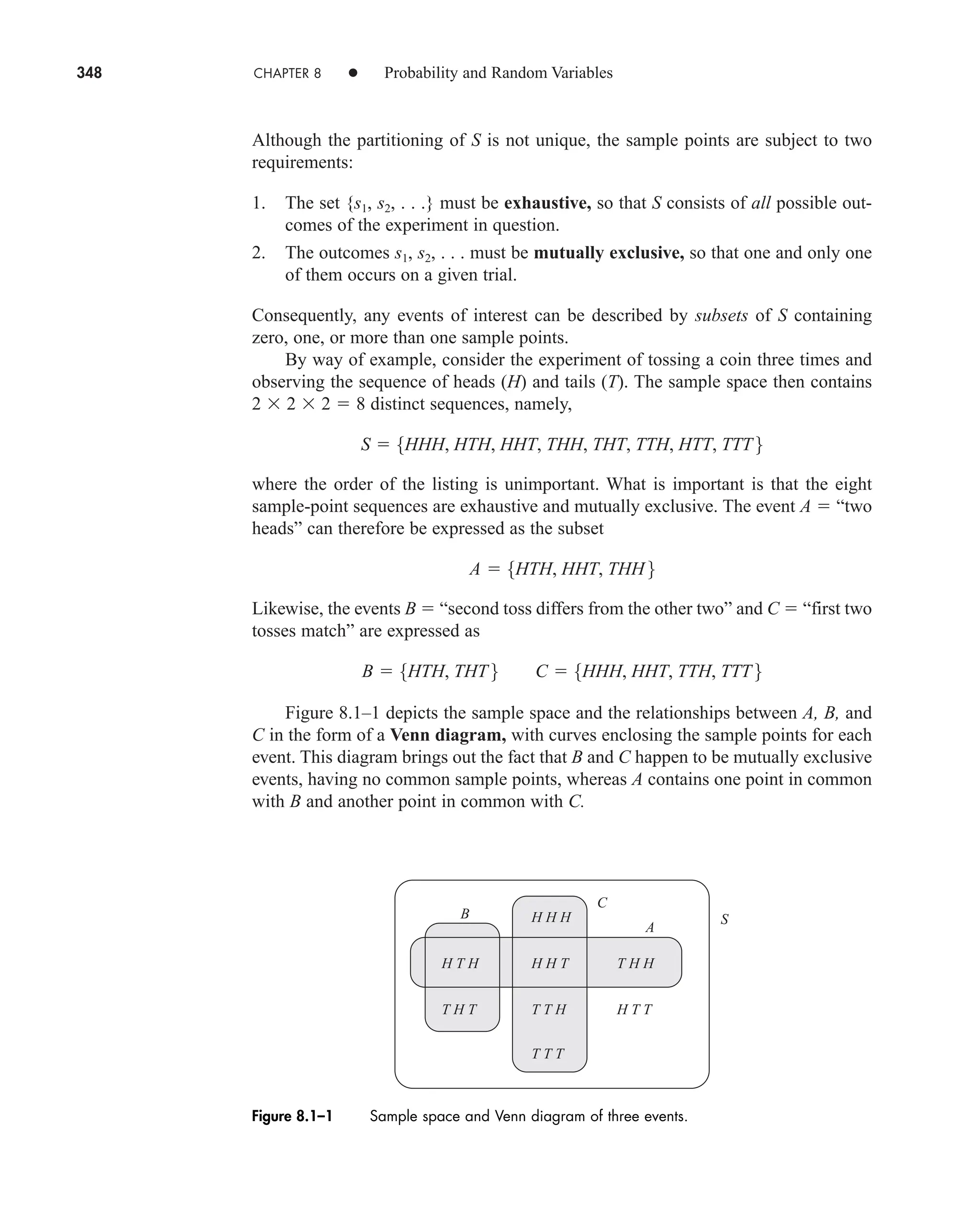

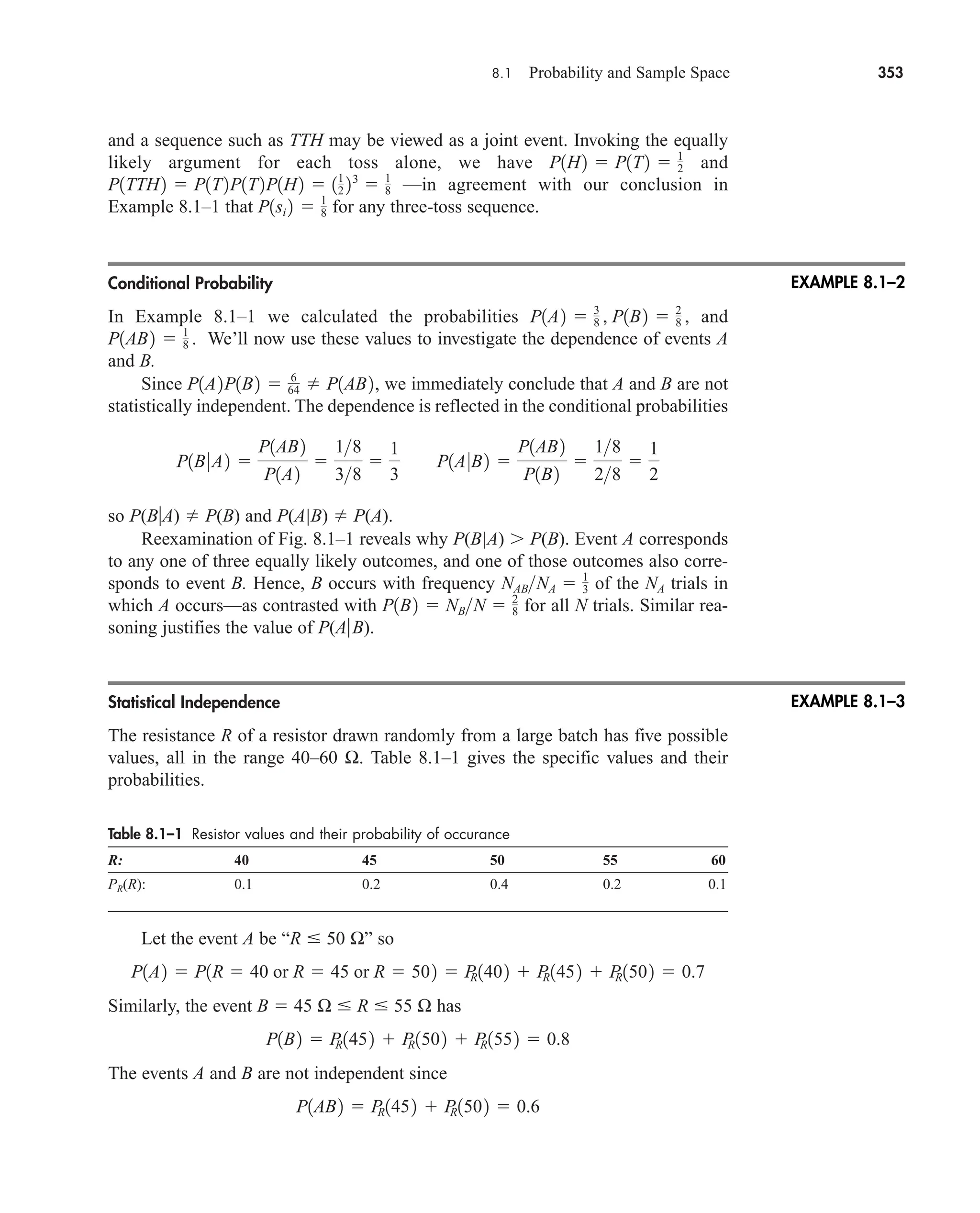
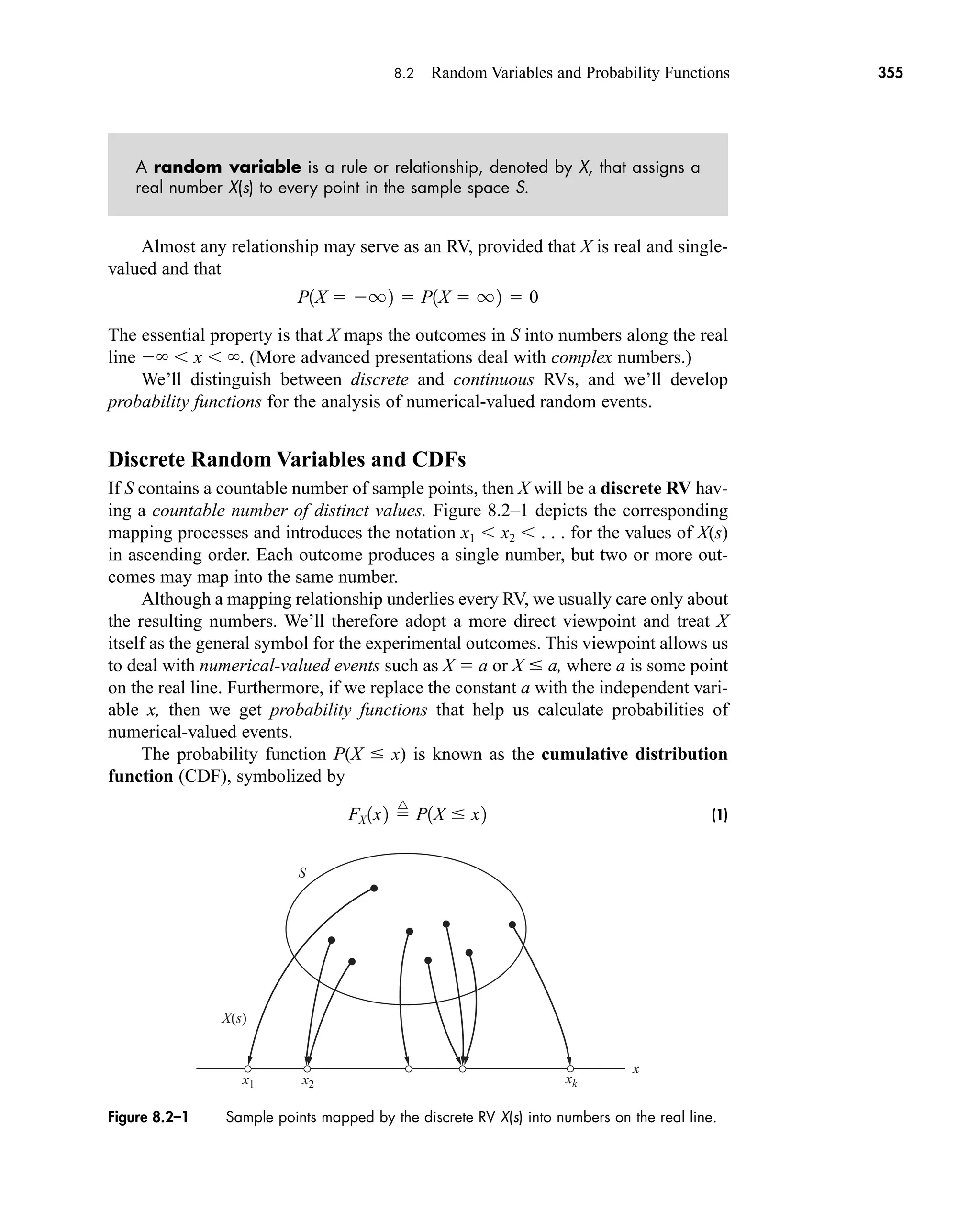
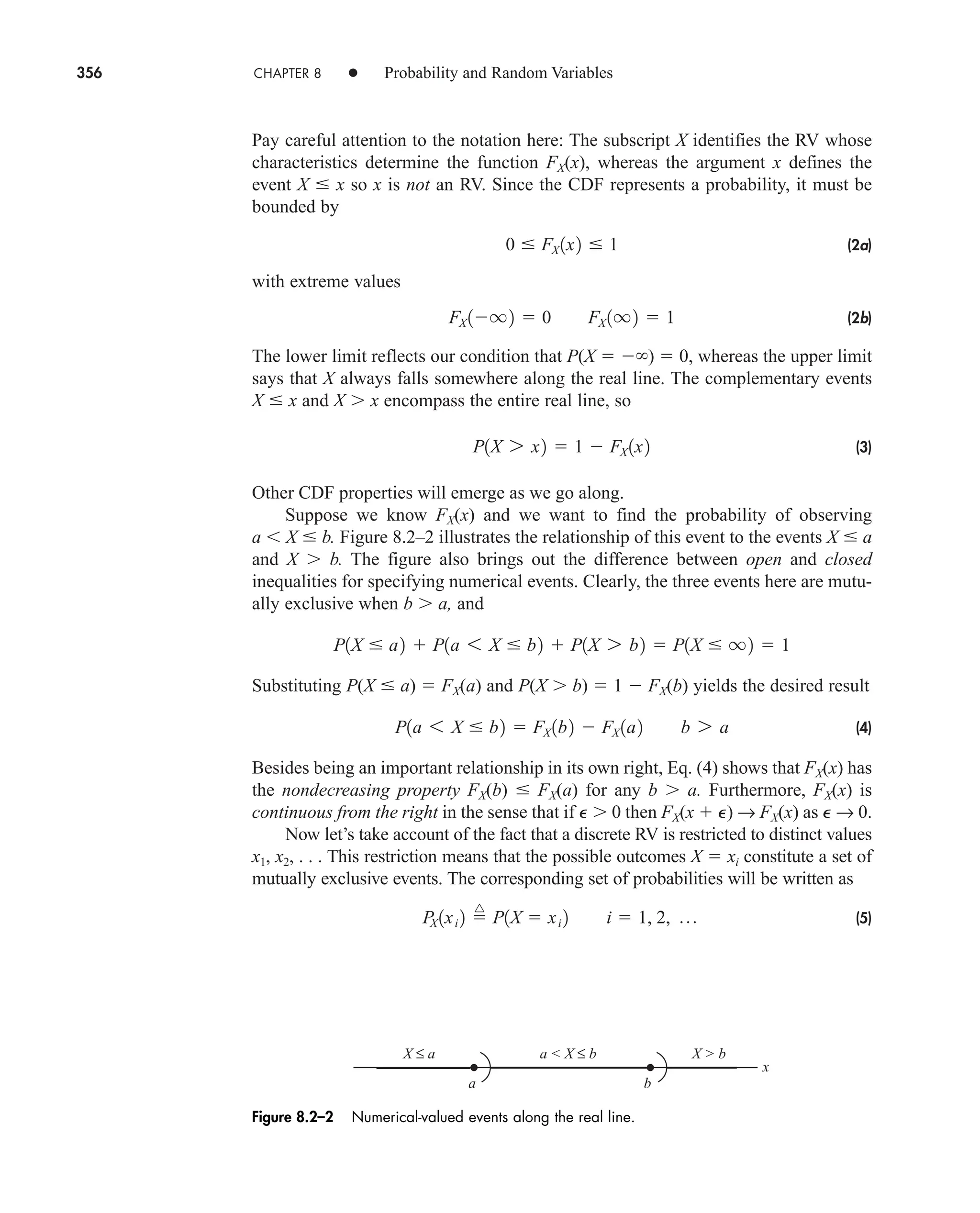
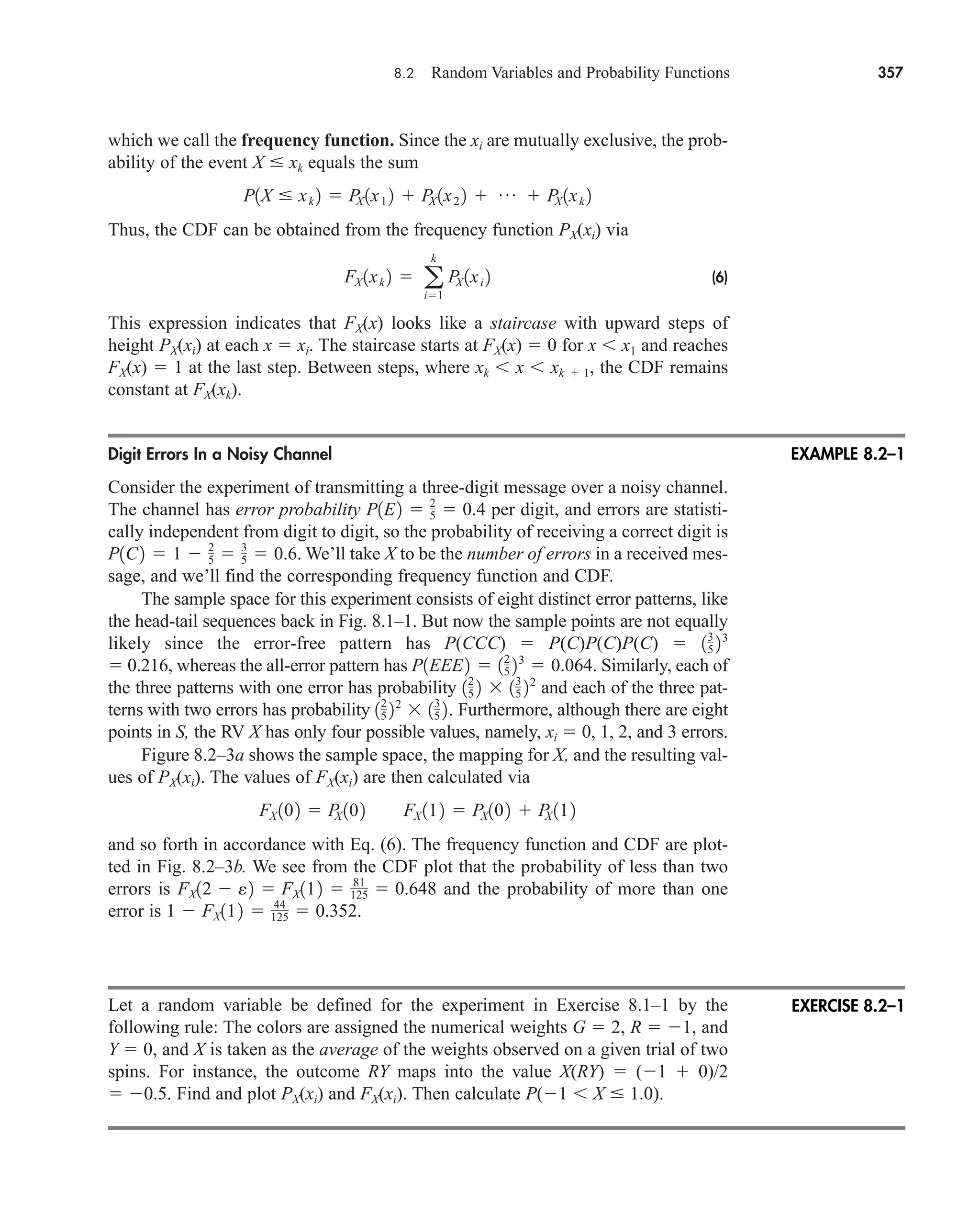
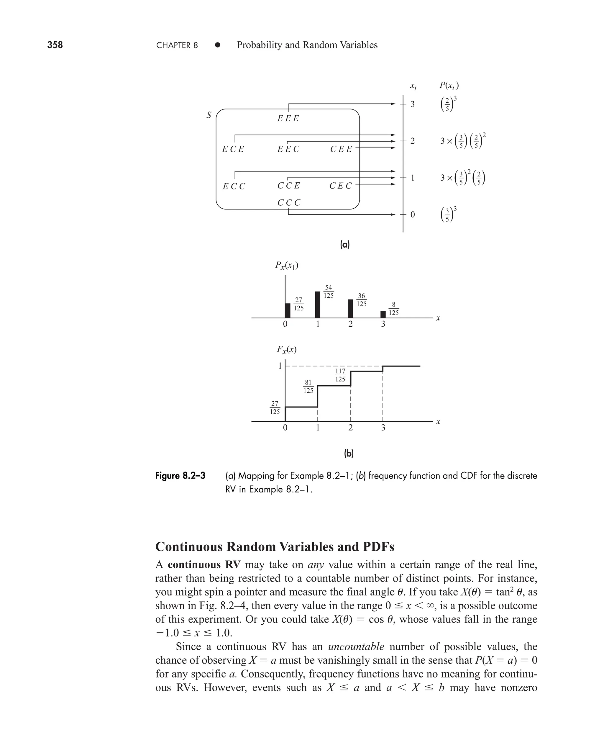
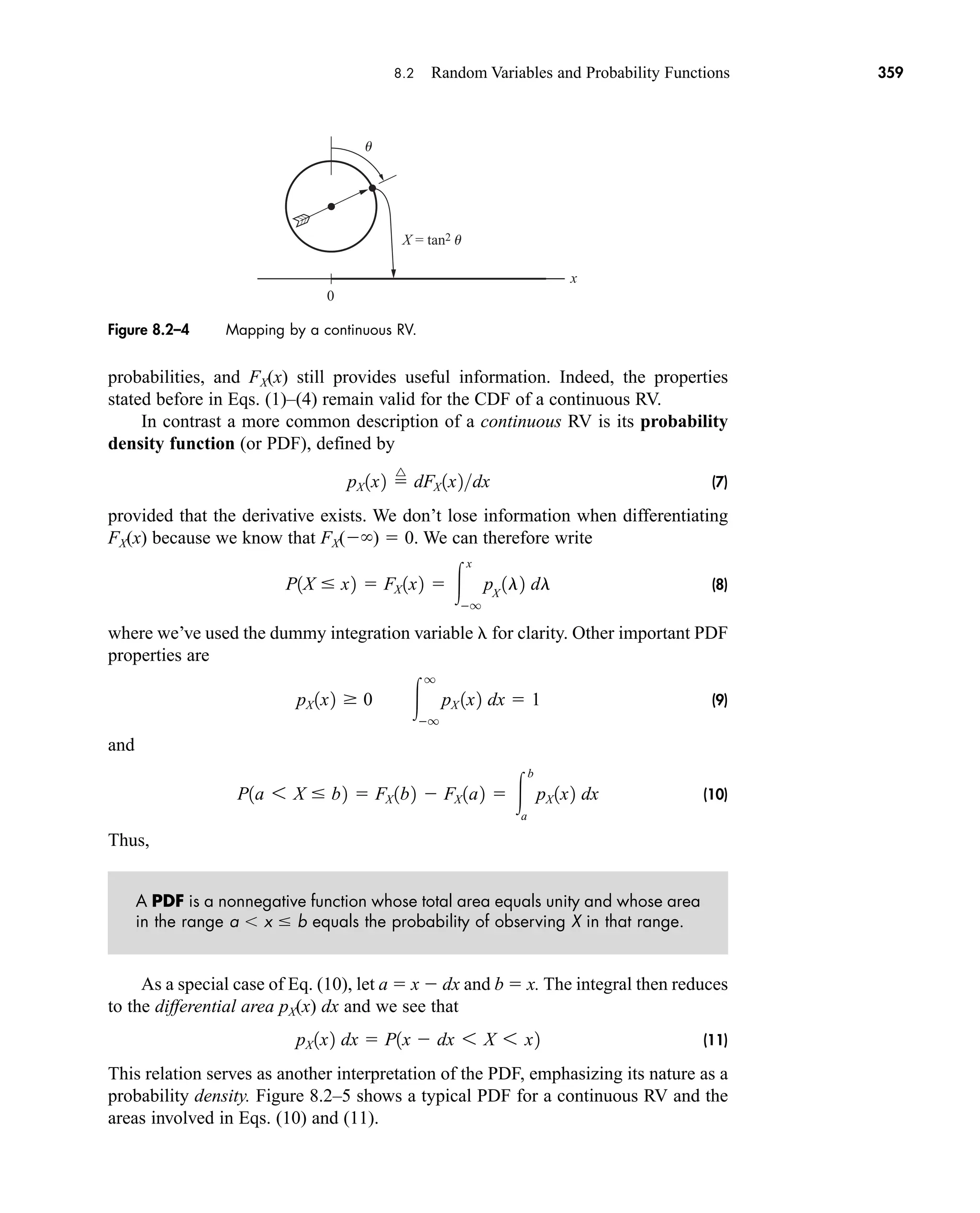
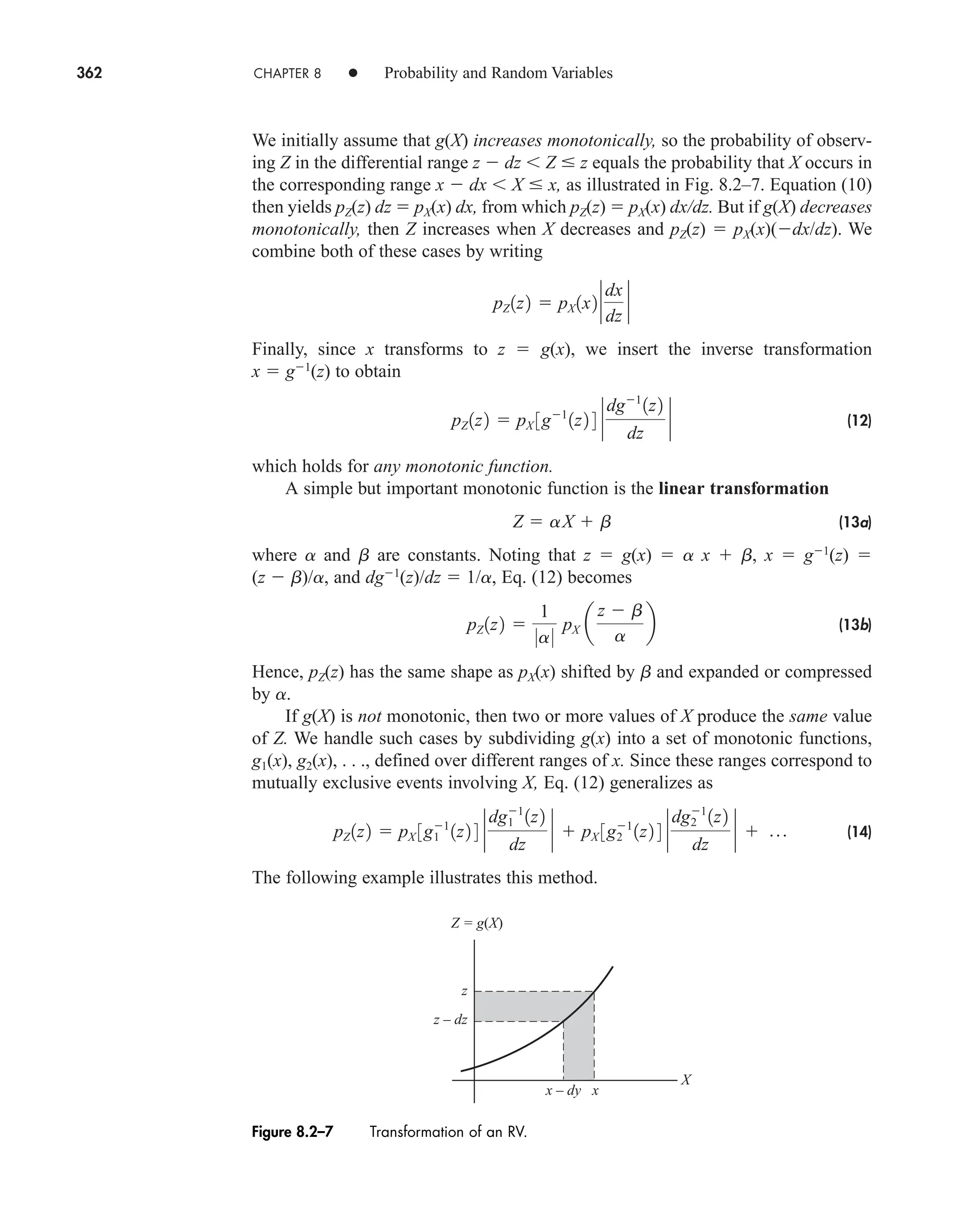
![8.2 Random Variables and Probability Functions 363
RV Transformation
Consider the transformation Z cos X with X being the uniformly distributed angle
from Example 8.2–2. The plot of Z versus X in Fig. 8.2–8a brings out the fact that Z
goes twice over the range 1 to 1 as X goes from 0 to 2p, so the transformation is
not monotonic.
To calculate pZ(z), we first subdivide g(x) into the two monotonic functions
which happen to be identical except for the defining ranges. For the range 0 x p,
we have with x g1
1 (z) cos1
z, so dg1
1 (z)/dz (1 z2
)1/2
and
pX[g1
1 (z)] over 1 z 1. The same results hold for p x 2p because
pX(x) still equals and g2(x) g1(x). Thus, from Eq. (14),
As illustrated in Fig. 8.2–8b, this PDF has peaks at z 1 because cos X occurs
more often near 1 than any other value when X is uniformly distributed over 2p
radians.
Find pZ(z) when and pX(x) is uniform over 0 x 4.
Joint and Conditional PDFs
Concluding our introduction to random variables, we briefly discuss the case of two
continuous RVs that can be observed simultaneously. A classic example of this
situation is the dart-throwing experiment, with X and Y taken as the rectangular coor-
dinates of the dart’s position relative to the center of the target.
Z 2X
pZ 1z2 2
1
2p
P 11 z212
P
1
p21 z2
1 z 1
1
2p
1
2p
pX1x2 1
2p
g21x2 cos x p 6 x 2p
g11x2 cos x 0 6 x p
EXAMPLE 8.2–3
(a) (b)
1/p
2p
p
1
–1
0 –1 0 1
g1 g2
Z = cos X
X z
pz(z)
Figure 8.2–8 Transformation of an RV where g(x) is not monotonic.
EXERCISE 8.2–3
car80407_ch08_345-390.qxd 1/13/09 4:07 PM Page 363
Rev.Confirming Pages](https://image.slidesharecdn.com/communicationsystemsanintro-a-241115060943-61721fa8/75/Communication_Systems__An_Intro_-_A-_Bruce_Carlson_-pdf-385-2048.jpg)
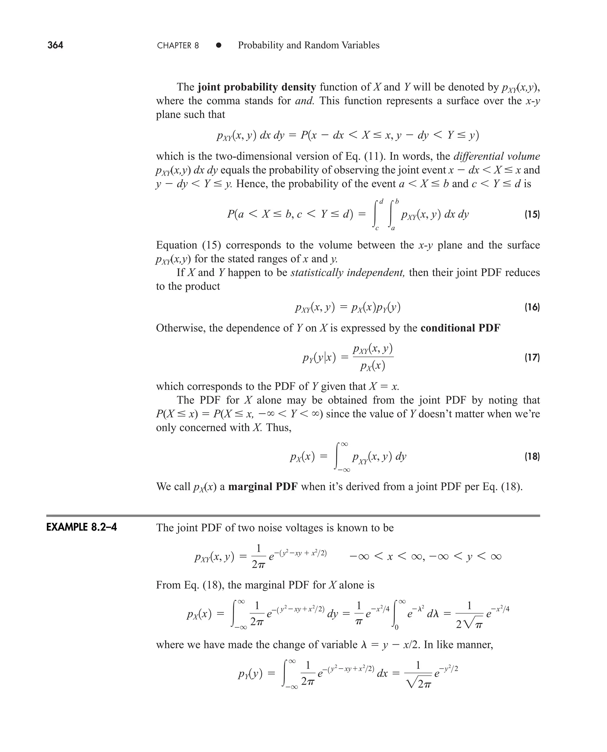
![8.3 Statistical Averages 365
Thus, X and Y are not independent since pX(x)pY(y) pXY(x,y). But Eq. (17) yields
the conditional PDFs
8.3 STATISTICAL AVERAGES
For some purposes, a probability function provides more information about an RV
than actually needed. Indeed, the complete description of an RV may prove to be an
embarrassment of riches, more confusing than illuminating. Thus, we often find it
more convenient to describe an RV by a few characteristic numbers. These numbers
are the various statistical averages presented here.
Means, Moments, and Expectation
The mean of the random variable X is a constant mX that equals the sum of the val-
ues of X weighted by their probabilities. This statistical average corresponds to an
ordinary experimental average in the sense that the sum of the values observed over
N W 1 trials is expected to be about NmX. For that reason, we also call mX the
expected value of X, and we write E[X] or to stand for the expectation operation
that yields mX.
To formulate an expression for the statistical average or expectation, we begin
by considering N independent observations of a discrete RV. If the event X xi
occurs Ni times, then the sum of the observed values is
(1a)
Upon dividing by N and letting N → , the relative frequency Ni/N becomes
P(X xi) PX(xi). Thus, the statistical average value is
(1b)
which expresses the mean of a discrete RV in terms of its frequency function PX(xi).
For the mean of a continuous RV, we replace PX(xi) with P(x dx X x)
pX(x) dx and pass from summation to integration so that
(2)
This expression actually includes Eq. (1b) as a special case obtained by writing the
discrete PDF as
pX 1x2 a
i
P
X 1xi 2d1x xi 2
mX
q
q
x pX
1x2 dx
mX a
i
xi P
X 1xi 2
N1x1 N2 x2p a
i
Ni xi
X
pY 1y0x2
1
2p
e
1y2
xyx2
4
2
pX 1x0y2
1
22p
e1y2
2 xyx2
2
2
car80407_ch08_345-390.qxd 12/11/08 5:55 PM Page 365](https://image.slidesharecdn.com/communicationsystemsanintro-a-241115060943-61721fa8/75/Communication_Systems__An_Intro_-_A-_Bruce_Carlson_-pdf-387-2048.jpg)
![366 CHAPTER 8 • Probability and Random Variables
Hence, when we allow impulses in the PDF, Eq. (2) applies to any RV—continuous,
discrete, or mixed. Hereafter, then, statistical averages will be written mostly in inte-
gral form with PDFs. The corresponding expressions for a strictly discrete RV are
readily obtained by substituting the frequency function in place of the PDF or, more
directly, by replacing the integration with the analogous summation.
When a function g(X) transforms X into another random variable Z, its expect-
ed value can be found from pX(x) by noting that the event X x transforms to
Z g(x), so
(3)
If g(X) Xn
, then E[Xn
] is known as the nth moment of X. The first moment, of
course, is just the mean value E[X] mX. The second moment E[X2
] or is called
the mean-square value, as distinguished from the mean squared Writing
out Eq. (3) with g(X) X2, we have
or, for a discrete RV,
The mean-square value will be particularly significant when we get to random sig-
nals and noise.
Like time averaging, the expectation in Eq. (3) is a linear operation. Thus, if a
and b are constants and if g(X) aX b, then
(4)
Although this result seems rather trivial, it leads to the not-so-obvious relation
since is a constant inside
Standard Deviation and Chebyshev’s Inequality
The standard deviation of X, denoted by sX, provides a measure of the spread of
observed values of X relative to mX. The square of the standard deviation is called the
variance, or second central moment, defined by
(5)
But a more convenient expression for the standard deviation emerges when we
expand (X mX)2
and invoke Eq. (4), so
E31X mX 22
4 E3X2
2mX X mX
2
4 X2
2mX X
mX
2
X2
mX
2
s2
X
^
E31X mX 22
4
E3X
X4.
X
E3X
X4 X
E3X4 X
2
E3aX b4 aX
b
X2
a
i
xi
2
PX 1xi 2
X2
q
q
x2
pX 1x2 dx
mX
2
X
2
.
X2
E3g1X2 4
q
q
g1x2pX 1x2 dx
car80407_ch08_345-390.qxd 1/13/09 4:07 PM Page 366
Rev.Confirming Pages](https://image.slidesharecdn.com/communicationsystemsanintro-a-241115060943-61721fa8/75/Communication_Systems__An_Intro_-_A-_Bruce_Carlson_-pdf-388-2048.jpg)
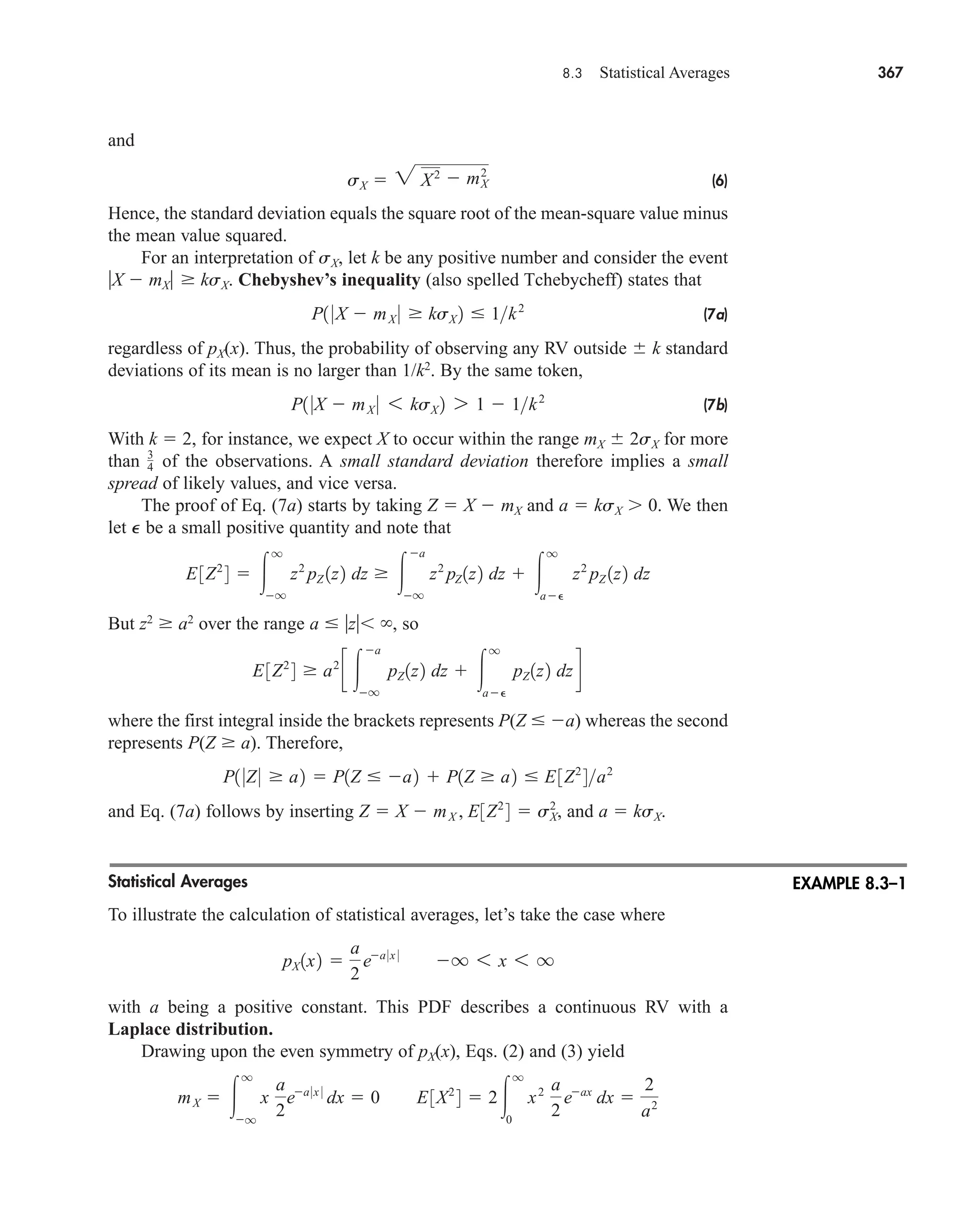
![368 CHAPTER 8 • Probability and Random Variables
Hence, from Eq. (6),
The probability that an observed value of a Laplacian RV falls within 2sX of
the mean is given by
as compared with the lower bound of 0.75 from Chebyshev’s inequality.
Let X have a uniform distribution over 0 X 2p, as in Example 8.2–2 (p. 360).
Calculate mX, and sX. What’s the probability of X mX 2sX?
Multivariate Expectations
Multivariate expectations involve two or more RVs, and they are calculated using
multiple integration over joint PDFs. Specifically, when g(X,Y) defines a function of
X and Y, its expected value is
(8)
However, we’ll restrict our attention to those cases in which the multiple integration
reduces to separate integrals.
First, suppose that X and Y are independent, so pXY(x,y) pX(x)pY(y). Assume
further that we can write g(X,Y) as a product in the form g(X,Y) gX(X)gY(Y). Equa-
tion (8) thereby becomes
(9)
If we take g(X,Y) XY, for instance, then gX(X) X and gY(Y) Y so E[XY]
E[X]E[Y] or
(10)
Hence, the mean of the product of independent RVs equals the product of their
means.
Next, consider the sum g(X,Y) X Y, where X and Y are not necessarily inde-
pendent. Routine manipulation of Eq. (8) now leads to E[X Y] E[X] E[Y] or
(11)
X Y X Y mX mY
XY X Y mX mY
E3gX 1X2 4E3gY 1Y 2 4
q
q
gX
1x2pX
1x2 dx
q
q
gY
1y2pY
1y2 dy
E3g1X, Y2 4
q
q
gX 1x2gY 1y2pX 1x2pY 1y2 dx dy
E3g1X, Y2 4
^
q
q
g1x, y2pXY 1x, y2 dx dy
X2
,
P1 0X 00 6 222a2
212a
212a
a
2
ea 0 x 0
dx 0.94
sX 2E3X2
4 m2
X 22a.
EXERCISE 8.3–1
car80407_ch08_345-390.qxd 1/13/09 4:07 PM Page 368
Rev.Confirming Pages](https://image.slidesharecdn.com/communicationsystemsanintro-a-241115060943-61721fa8/75/Communication_Systems__An_Intro_-_A-_Bruce_Carlson_-pdf-390-2048.jpg)
![8.3 Statistical Averages 369
Hence, the mean of the sum equals the sum of the means, irrespective of statistical
independence.
Finally, let Z X Y so we know that mZ mX mY. But what’s the variance
? To answer that question we calculate the mean-square value E[Z2
] via
Thus,
The last term of this result vanishes when Eq. (10) holds, so the variance of the sum
of independent RVs is
(12)
Equations (9) through (12) readily generalize to include three or more RVs.
Keep in mind, however, that only Eq. (11) remains valid when the RVs are not
independent.
Sample Mean and Frequency of Occurrence
Let X1, X2, . . . XN be sample values obtained from N independent observations of a
random variable X having mean mX and variance Each sample value is an RV,
and so is the sum
and the sample mean
and sample variance
We’ll investigate the statistical properties of m, and we’ll use them to reexamine the
meaning of probability.
From Eqs. (11) and (12) we have and sX
2
NsX
2
. Thus, whereas
Since the spread of the sample mean decreases with increasing N,
and m approaches mX as N → . Furthermore, from Chebyshev’s inequality, the
probability that m differs from mX by more than some positive amount e is upper-
bounded by
P1 0m mX 0 P2 sX
2
NP2
sm sX2N,
sm
2
E31m m
22
4
1
N2 E31Z Z 22
4
1
N 2 sZ
2
1
N
sX
2
m
ZN mX,
Z X1 X2 p XN NmX
sm
B
1
N a
N
i1
1xi m22
m ZN
Z X1 X2 p XN
sX
2
.
sZ
2
sX
2
sY
2
sZ
2
Z2
1mX mY 22
1X2
mX
2
2 1Y2
mY
2
2 21XY mxmY 2
Z2
E3X2
2XY Y2
4 X2
2XY Y2
sZ
2
EXAMPLE 8.3–2
car80407_ch08_345-390.qxd 12/11/08 5:55 PM Page 369](https://image.slidesharecdn.com/communicationsystemsanintro-a-241115060943-61721fa8/75/Communication_Systems__An_Intro_-_A-_Bruce_Carlson_-pdf-391-2048.jpg)
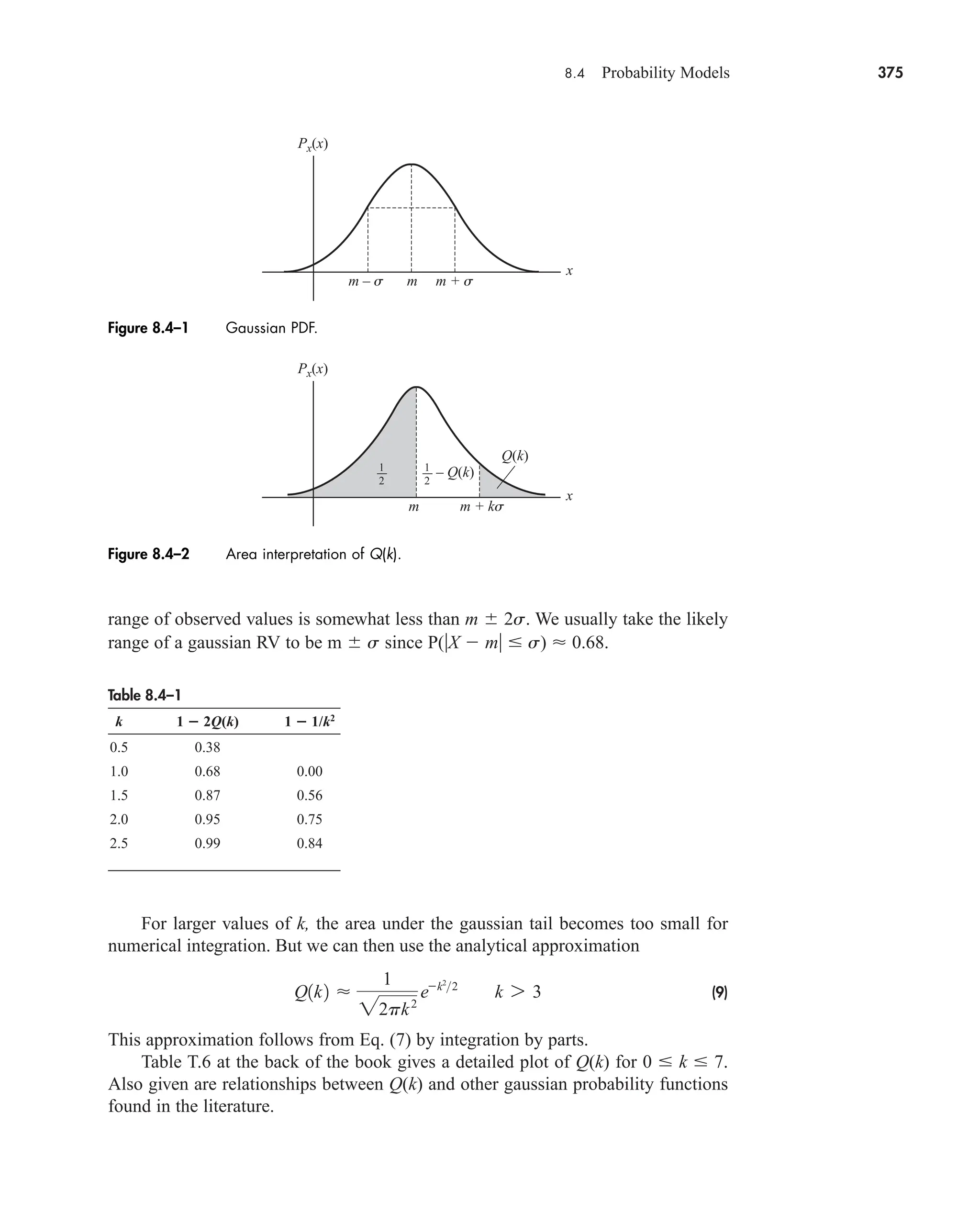
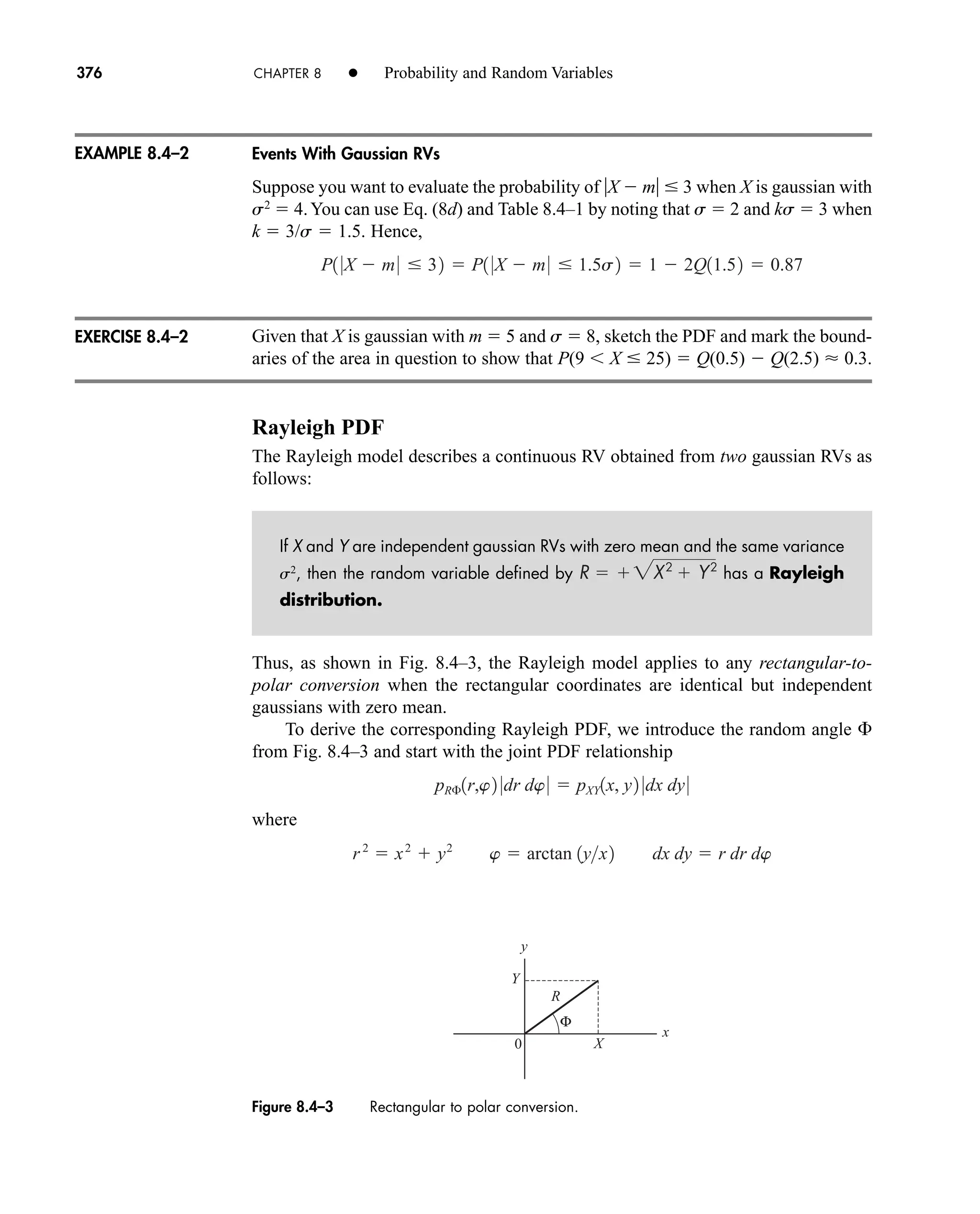
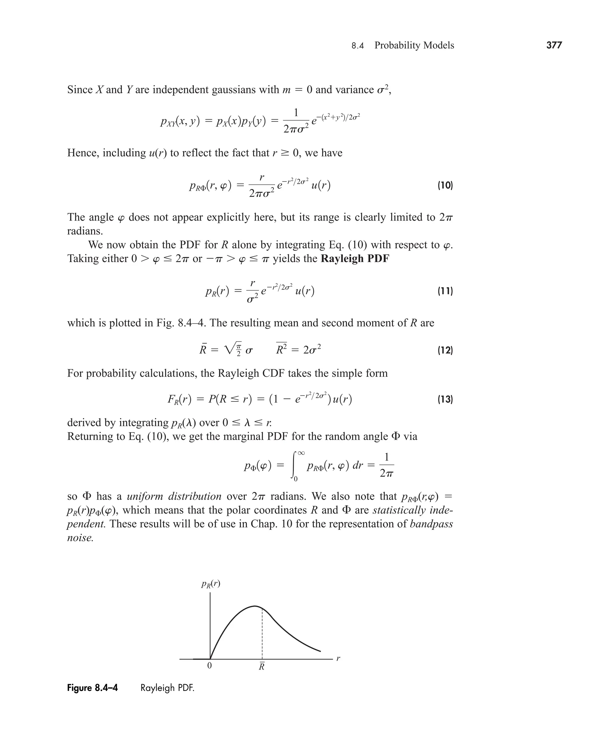
![378 CHAPTER 8 • Probability and Random Variables
Rayleigh Event
Suppose you throw darts at a target whose bull’s eye has a radius of 3 cm. If the rec-
tangular coordinates of the impact points are gaussianly distributed about the origin
with spread s 4 cm in either direction, then your probability of hitting the bull’s
eye is given by Eq. (13) as
Derive Eq. (13) from Eq. (11).
Bivariate Gaussian Distribution
Lastly, we want to investigate the joint PDF of two gaussian RVs that are neither
identically distributed nor independent. As preparation, we first introduce a general
measure of interdependence between any two random variables.
Let X and Y be arbitrarily distributed with respective means and variances
and The degree of dependence between them is expressed by the
correlation coefficient
(14)
where the expectation E[(X mX)(Y mY)] is called the covariance of X and Y. At
one extreme, if X and Y are statistically independent, then E[(X mX)(Y mY)]
E[(X mX)]E(Y mY)] 0 so the covariance equals zero and r 0. At the other
extreme, if Y depends entirely upon X in the sense that Y aX, then
and the covariance equals so r 1. Thus, the correlation coefficient ranges
over 1 r 1, and r reflects the degree of interdependence.
When X and Y are interdependent gaussian RVs, their joint PDF is given by the
bivariate gaussian model
(15a)
with
(15b)
This formidable-looking expression corresponds to a bell-shaped surface over the x-y
plane, the peak being at x mX and y mY.
If r 0, then the last term of Eq. (15b) disappears and pXY(x,y) pX(x)pY(y).
We thus conclude that
• Uncorrelated gaussian RVs are statistically independent.
f 1x, y2
1x mX 22
2sX
2
1y mY 22
2sY
2
1x mX 21y mY 2r
sX sY
pXY 1x, y2
1
2psX sY 21 r2
ef 1x, y211r2
2
asX
2
sY
2
1asX 22
r
^ 1
sX sY
E31X mX 21Y mY 2 4
sY
2
.
mX , mY , sX
2
,
P1R 32 1 e932
25%
EXAMPLE 8.4–3
EXERCISE 8.4–3
car80407_ch08_345-390.qxd 1/13/09 4:07 PM Page 378
Rev.Confirming Pages](https://image.slidesharecdn.com/communicationsystemsanintro-a-241115060943-61721fa8/75/Communication_Systems__An_Intro_-_A-_Bruce_Carlson_-pdf-400-2048.jpg)
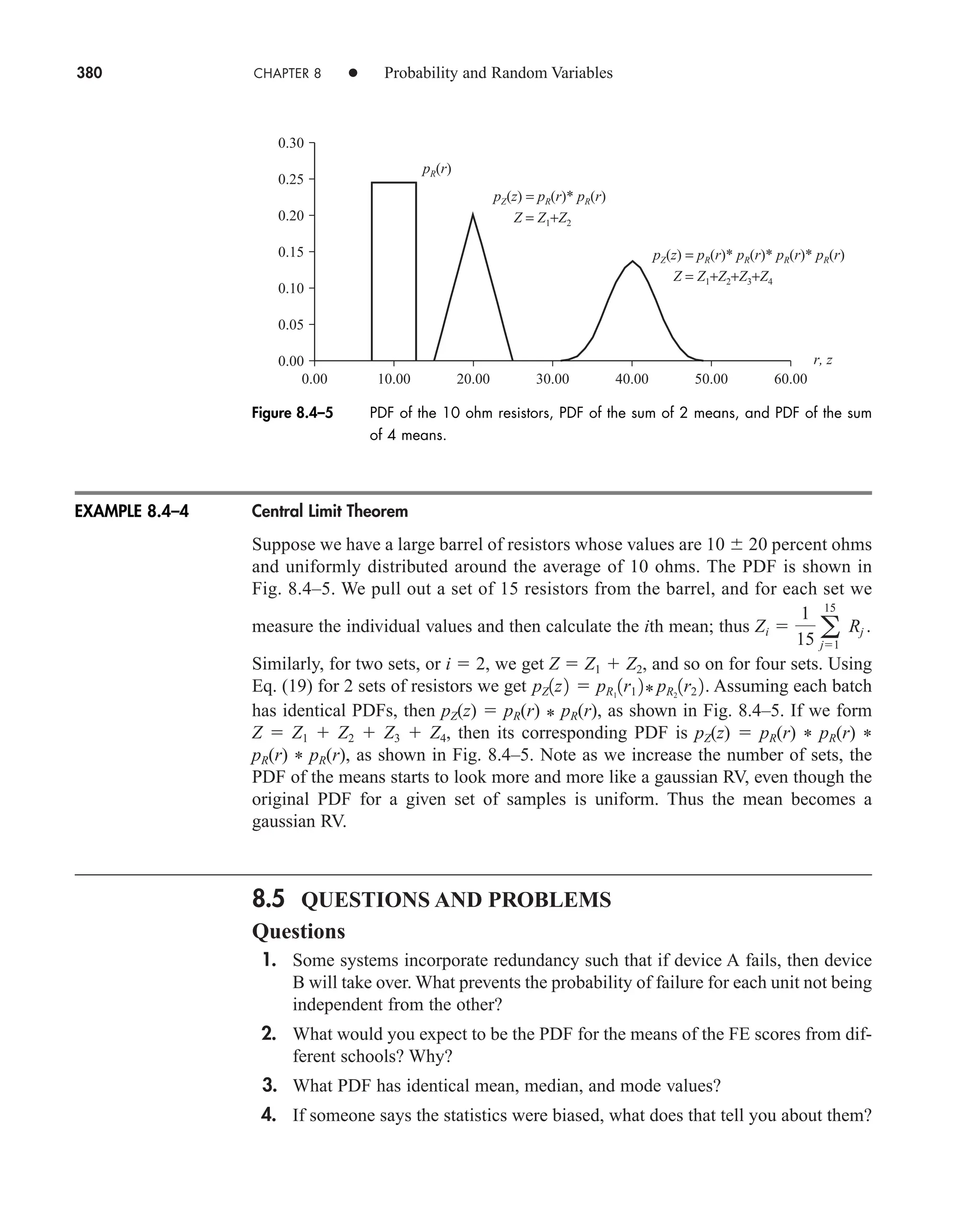
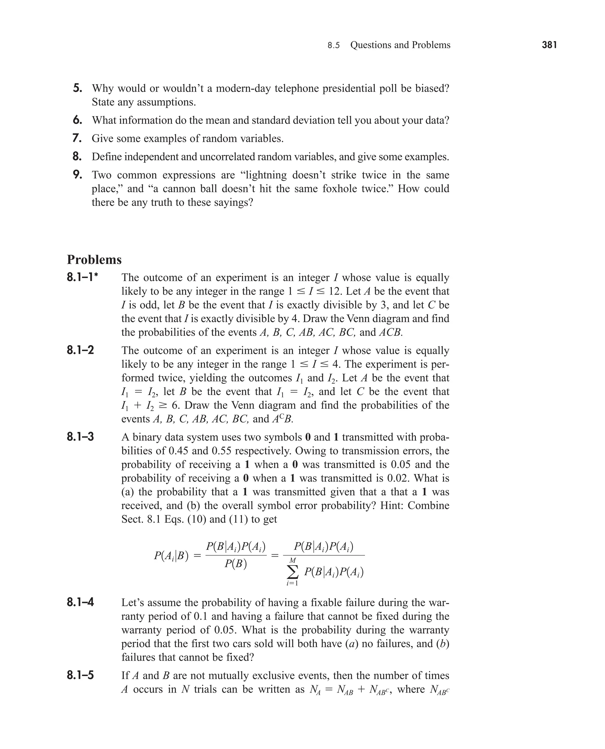
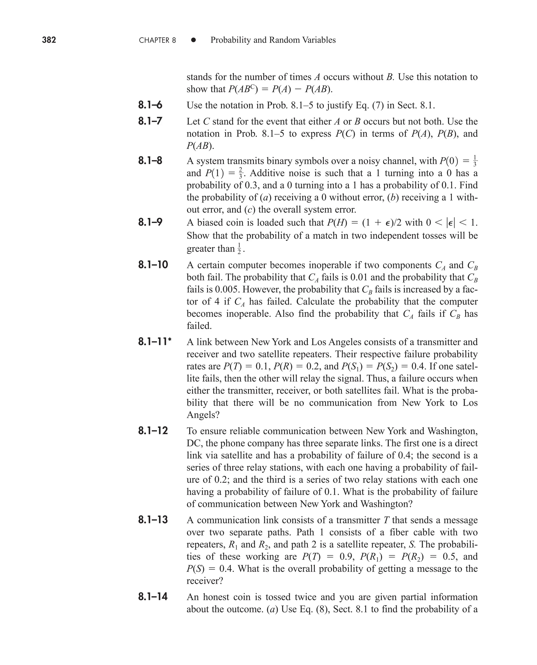
![384 CHAPTER 8 • Probability and Random Variables
8.2–6 Do Prob. 8.2–5 with
8.2–7 Given that FX(x) (p 2 tan1
x)/2p, find the CDF and PDF of the
random variable Z defined by Z 0 for X 0 and Z X for X 0.
8.2–8‡
Do Prob. 8.2–7 with Z –1 for X 0 and Z X for X 0.
8.2–9* Let pX(x) 2e2x
u(x). Find the PDF of the random variable defined by
the transformation Z 2X 5. Then sketch both PDFs on the same set
of axes.
8.2–10 Do Prob. 8.2–9 with Z –2X 1.
8.2–11 Let X have a uniform PDF over 1 x 3. Find and sketch the PDF
of Z defined by the transformation
8.2–12 Do Prob. 8.2–11 with Z X.
8.2–13‡
Do Prob. 8.2–11 with
8.2–14 Consider the square-law transformation Z X2
. Show that
8.2–15 Let pX(x) be a gaussian pdf with zero mean and sX. Find the PDF of the
random variable defined by the transformation of Y e2X
u(X).
8.2–16* Find pY(y) when pXY(x,y) yey(x 1)
u(x)u(y). Then show that X and Y
are not statistically independent, and find pX(x|y).
8.2–17 Do Prob. 8.2–16 with pXY(x,y) [(x y)2
/40]Π(x/2)Π(y/6).
8.2–18 Show that Explain why this must be true.
8.2–19 Obtain an expression for pY(yx) in terms of pX(xy) and pY(y).
8.3–1* Find the mean, second moment, and standard deviation of X when
pX(x) aeax
u(x) with a 0.
8.3–2 Find the mean, second moment, and standard deviation of X when
pX(x) a2
xeax
u(x) with a 0.
8.3–3 Find the mean, second moment, and standard deviation of X when
8.3–4 A discrete RV has two possible values, a and b. Find the mean, second
moment, and standard deviation in terms of p P(X a).
pX 1x2
22
p31 1x a244
q
q
px1x0y2 dx 1.
pZ 1z2
1
22z
3 pX 12z2 pX 12z 2 4u1z2
Z 20X 0 .
Z 2X 1.
FX 1x2 µ
0 x 0
K sin px40 0 6 x 10
K sin p4 x 7 10
car80407_ch08_345-390.qxd 12/16/08 6:12 PM Page 384](https://image.slidesharecdn.com/communicationsystemsanintro-a-241115060943-61721fa8/75/Communication_Systems__An_Intro_-_A-_Bruce_Carlson_-pdf-406-2048.jpg)
![8.5 Questions and Problems 385
8.3–5* A discrete RV has K equally likely possible values, 0, a, 2a,. . . (K 1)a.
Find the mean, second moment, and standard deviation.
8.3–6 Find the mean, second moment, and standard deviation of Y a cos X,
where a is a constant and X has a uniform PDF over u x u 2p.
8.3–7 Do Prob. 8.3–6 for the case when X has a uniform PDF over
u x u p.
8.3–8 Let Y aX b. Show that sY asX.
8.3–9* Let Y X b. What value of b minimizes E[Y2
]?
8.3–10‡
Let X be a nonnegative continuous RV and let a be any positive constant.
By considering E[X], derive Markov’s inequality P(X a) mX/a.
8.3–11 Use E[(X Y)2
] to obtain upper and lower bounds on E[XY] when X and
Y are not statistically independent.
8.3–12 The covariance of X and Y is defined as CXY E[(X mX)(Y mY)].
Expand this joint expectation and simplify it for the case when: (a) X and
Y are statistically independent; (b) Y is related to X by Y aX b.
8.3–13 Let received signal Y X N, where X and N are the desired signal and
zero- mean additive noise respectively. Assume that X and N are
independent, and statistics and mN are known. Determine an
estimator a that X aY minimizes the mean squared error ε2
E[(X aY)2
]
8.3–14 In linear estimation we estimate Y from X by writing aX b.
Obtain expressions for a and b to minimize the mean square error
8.3–15 Show that the nth moment of X can be found from its characteristic func-
tion via
8.3–16* Obtain the characteristic function of X when pX(x) aeax
u(x) with
a 0. Then use the relation in Prob. 8.3–15 to find the first three
moments.
8.3–17 Let X have a known PDF and let Y g(X), so
If this integral can be rewritten in the form
£Y 1n2
q
q
ejnl
h1l2 dl
£Y 1n2 E3ejng1X 2
4
q
q
e
jng1x2
pX
1x2 dx
E3Xn
4 jn
dn
£X1n2
dnn `
n 0
P2
E31Y Y
22
4.
Y
sN
2
, sX
2
, mX ,
car80407_ch08_345-390.qxd 12/11/08 5:55 PM Page 385](https://image.slidesharecdn.com/communicationsystemsanintro-a-241115060943-61721fa8/75/Communication_Systems__An_Intro_-_A-_Bruce_Carlson_-pdf-407-2048.jpg)
![386 CHAPTER 8 • Probability and Random Variables
then pY(y) h(y). Use this method to obtain the PDF of Y X2
when
pX(x)
8.3–18‡
Use the method in Prob. 8.3–17 to obtain the PDF of Y sin X when X
has a uniform PDF over x p/2.
8.3–19 Early component failures can be modeled by an exponential PDF with
pX(x) aeax
u(x), with the mean time to failure of mX 6 months.
(a) Derive the PDF function and determine and (b) determine the
probability of failure after 12 months.
8.4–1* Ten honest coins are tossed. What’s the likely range of the number of
heads? What’s the probability that there will be fewer than three heads?
8.4–2 Do Prob. 8.4–1 with biased coins having P(H) 3/5.
8.4–3 The one-dimensional random walk can be described as follows. An ine-
briated man walking in a narrow hallway takes steps of equal length l. He
steps forward with probability or backwards with probability
Let X be his distance from the starting point after 100 steps.
Find the mean and standard deviation of X.
8.4–4 A noisy transmission channel has per-digit error probability a 0.01.
Calculate the probability of more than one error in 10 received digits.
Repeat this calculation using the Poisson approximation.
8.4–5* A radioactive source emits particles at the average rate of 0.5 particles
per second. Use the Poisson model to find the probability that: (a) exact-
ly one particle is emitted in two seconds; (b) more than one particle is
emitted in two seconds.
8.4–6‡
Show that the Poisson distribution in Eq. (5), Sect. 8.4, yields E[I] m
and E[I2
] m2
m. The summations can be evaluated by writing the
series expansion for em
and differentiating it twice.
8.4–7 Observations of a noise voltage X are found to have a gaussian distribu-
tion with m 100 and s 2. Evaluate and the probability that X
falls outside the range m s.
8.4–8 A gaussian RV has and Evaluate the probabilities of the
events X 5 and 2 X 5.
8.4–9* A gaussian RV has E[X] 10 and E[X2
] 500. Find P(X 20),
P(10 X 20), P(0 X 20), and P(X 0).
8.4–10 When a binomial CDF has n W 1, it can be approximated by a gaussian
CDF with the same mean and variance. Suppose an honest coin is tossed
100 times. Use the gaussian approximation to find the probability that
(a) heads occurs more than 70 times; (b) the number of heads is between
40 and 60.
8.4–11 Let X be a gaussian RV with mean m and variance s2
. Write an expres-
sion in terms of the Q function for P(a X b) with a m b.
X2
13.
X 2
X2
1 a 1
4.
a 3
4
sX
2
,
2axeax 2
u1x2.
car80407_ch08_345-390.qxd 12/11/08 5:55 PM Page 386](https://image.slidesharecdn.com/communicationsystemsanintro-a-241115060943-61721fa8/75/Communication_Systems__An_Intro_-_A-_Bruce_Carlson_-pdf-408-2048.jpg)
![8.5 Questions and Problems 387
8.4–12 Consider a home burglar system that uses motion detectors such that
movement detected above a specific threshold will trigger an alarm.
There is always some random motion in the house, but an intruder
increases the level that triggers the alarm. The random motion has a
Rayleigh PDF with s 1.5 V2
. Testing shows that an intruder causes a
random motion with a voltage output intruder, that has a gaussian distri-
bution with a mean and standard deviation of 7.5 and 2.0 V respective-
ly. If the threshold is low enough, the random motion can reach a level
to trigger a false alarm. Determine the threshold level such that the
probability of a false alarm is P(FA) 0.005. Then calculate the
corresponding probability of detecting an intruder.
8.4–13* Consider the burglar system of Prob. 8.4–12. What would the threshold
be if we wanted the probability of detection to be greater than 0.99, and
what would be the corresponding false alarm probability?
8.4–14 A digital signal whereby a “1” → 5 volts, and a “0” → 0 volts is trans-
mitted over a channel that has been corrupted by zero-mean gaussian
noise with s 2 volts. Furthermore, the data is such that and
The detector’s threshold is such that, if the received signal is
above 3 volts, it is interpreted as a logic 1, otherwise it is considered a
logic 0. (a) Calculate the overall probability of error Pe for your system,
and (b) suggest ways to reduce Pe.
8.4–15 Do Prob 8.4–14 with the noise having a uniform PDF whose range is
4 volts.
8.4–16* Do Prob 8.4–14 with the noise having a PDF of
8.4–17 As course instructor you have decided that the final grades have to fit a
normal or gaussian distribution such that 5% of the class are assigned
grades of A and F, 20% are assigned grades B and D, and the remaining
50% are assigned a grade of C. If the class statistics are mX 60 and
s 15, what are the breakpoints for grades A–F?
8.4–18 A professional licensing exam is set up so that the passing grade is cal-
culated to be a score greater than 1.5 standard deviations below the mean.
What is the pass percentage for a given exam that has an average of 60
and standard deviation of 20? Assume grades have a normal distribution.
8.4–19 A random noise voltage X is known to be gaussian with E[X] 0 and
E[X2
] 9. Find the value of c such that X c for (a) 90 percent of the
time; (b) 99 percent of the time.
8.4–20 Write to show that the approximation in
Eq. (9), Sect. 8.4, is an upper bound on Q(k). Then justify the approxi-
mation for k W 1.
el2
2
dl 11l2d1el2
2
2
pN1n2
1
2
e0x0
.
P102
1
4
.
P112
3
4
car80407_ch08_345-390.qxd 12/11/08 5:55 PM Page 387](https://image.slidesharecdn.com/communicationsystemsanintro-a-241115060943-61721fa8/75/Communication_Systems__An_Intro_-_A-_Bruce_Carlson_-pdf-409-2048.jpg)
![388 CHAPTER 8 • Probability and Random Variables
8.4–21 Let X be a gaussian RV with mean m and variance s2
. (a) Show that
E[(X m)n] 0 for odd n. (b) For even n, use integration by parts to
obtain the recursion relation
Then show for n 2, 4, 6, . . . that
8.4–22 Let X be a gaussian RV with mean m and variance s2
. Show that its
characteristic function is
8.4–23 Let Z X Y, where X and Y are independent gaussian RVs with differ-
ent means and variances. Use the characteristic function in Prob. 8.4–22
to show that Z has a gaussian PDF. Then extrapolate your results for
where the Xi are mutually independent gaussian RVs.
8.4–24 A random variable Y is said to be log-normal if the transformation
X ln Y yields a gaussian RV. Use the gaussian characteristic function
in Prob. 8.4–22 to obtain E[Y] and E[Y2
] in terms of mX and Do not
find the PDF or characteristic function of Y.
8.4–25 Let Z X2
, where X is a gaussian RV with zero mean and variance s2
.
(a) Use Eqs. (3) and (13), Sect. 8.3, to show that
(b) Apply the method in Prob. 8.3–17 to find the first three moments of Z.
What statistical properties of X are obtained from these results?
8.4–26 The resistance R of a resistor drawn randomly from a large batch is
found to have a Rayleigh distribution with Write the PDF pR(r)
and evaluate the probabilities of the events R 6 and 4.5 R 5.5.
8.4–27 The noise voltage X at the output of a rectifier is found to have a
Rayleigh distribution with Write the PDF pX(x) and evaluate
P(X 3), P(X 4), and P(3 X 4).
8.4–28 Certain radio channels suffer from Rayleigh fading such that the
received signal power is a random variable Z X2
and X has a Rayleigh
distribution. Use Eq. (12), Sect. 8.2, to obtain the PDF
where m E[Z]. Evaluate the probability P(Z km) for k 1 and
k 0.1.
pZ 1z2
1
m
ezm
u1z2
X2
18.
R2
32.
£Z 1n2 11 j2s2
n212
sX
2
.
Z
1
n a
n
i1
Xi
£X 1n2 es2
n2
2
e jmn
.
E31X m2n
4 1 # 3 # 5 p 1n 12sn
E31X m2n
4 1n 12s2
E31X m2n2
4
car80407_ch08_345-390.qxd 12/11/08 5:55 PM Page 388](https://image.slidesharecdn.com/communicationsystemsanintro-a-241115060943-61721fa8/75/Communication_Systems__An_Intro_-_A-_Bruce_Carlson_-pdf-410-2048.jpg)
![8.5 Questions and Problems 389
8.4–29‡
Let R1 and R2 be independent Rayleigh RVs with E[R1
2
] E[R2
2
] 2s2
.
(a) Use the characteristic function from Prob. 8.4–18 to obtain the PDF of
A R1
2
. (b) Now apply Eq. (15), Sect. 8.3, to find the PDF of W R1
2
R2
2
.
8.4–30 Let the bivariate gaussian PDF in Eq. (15), Sect. 8.4, have mX mY 0
and sX sY s. Show that pY(y) and pX(xy) are gaussian functions.
8.4–31 Find the PDF of Z X 3Y when X and Y are gaussian RVs with
mX 6, mY –2, sX sY 4, and E[XY] 22.
8.4–32 Let X Y2
, so X and Y are not independent. Nevertheless, show that they
are uncorrelated if the PDF of X has even symmetry.
car80407_ch08_345-390.qxd 12/11/08 5:55 PM Page 389](https://image.slidesharecdn.com/communicationsystemsanintro-a-241115060943-61721fa8/75/Communication_Systems__An_Intro_-_A-_Bruce_Carlson_-pdf-411-2048.jpg)

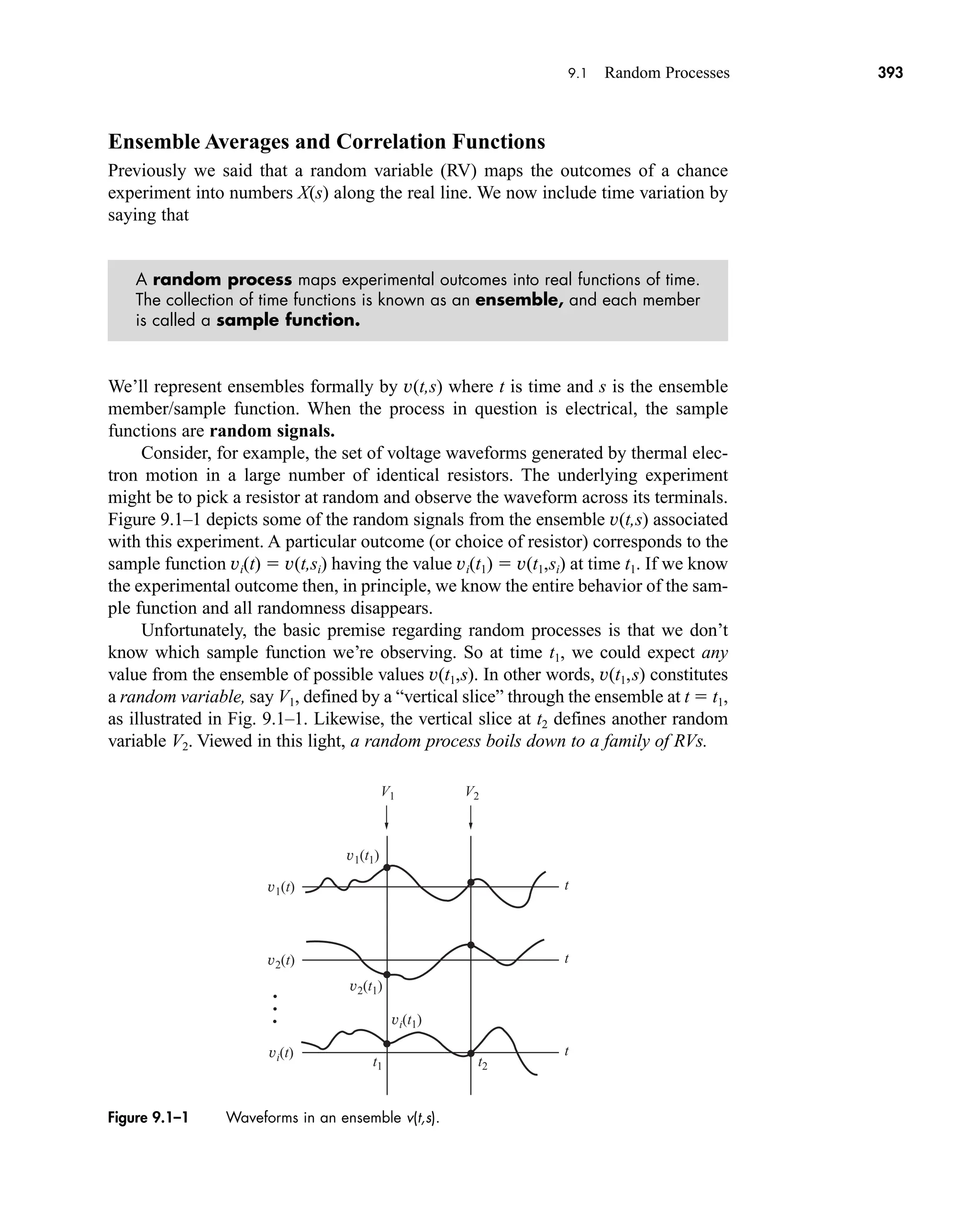
![394 CHAPTER 9 • Random Signals and Noise
Now let’s omit s and represent the random process by v(t), just as we did when
we used X for a single random variable. The context will always make it clear
when we’re talking about random processes rather than nonrandom signals, so
we’ll not need a more formal notation. (Some authors employ boldface letters or
use V(t) for the random process and for the random variables.) Our streamlined
symbol v(t) also agrees with the fact that we hardly ever know nor care about the
details of the underlying experiment. What we do care about are the statistical
properties of v(t).
For a given random process, the mean value of v(t) at arbitrary time t is
defined as
(1)
Here, E[v(t)] denotes an ensemble average obtained by averaging over all the sam-
ple functions with time t held fixed at an arbitrary value. Setting t t1 then yields
which may differ from
To investigate the relationship between the RVs V1 and V2 we define the
autocorrelation function
(2)
where the lowercase subscript has been used to be consistent with our previous work
in Chapter 3. This function measures the relatedness or dependence between V1 and
V2. If they happen to be statistically independent, then However, if
t2 t1, then V2 V1 and More generally, setting t2 t1 t yields
which is the mean-square value of v(t) as a function of time.
Equations (1) and (2) can be written out explicitly when the process in question
involves an ordinary random variable X in the functional form
Thus, at any time ti, we have the RV transformation Vi g(X,ti). Consequently,
knowledge of the PDF of X allows you to calculate the ensemble average and the
autocorrelation function via
(3a)
(3b)
Equations (3a) and (3b) also generalize to the case of a random process defined in
terms of two or more RVs. If v(t) g(X,Y,t), for instance, then Eq. (3b) becomes
Rv(t1,t2) E[g(X,Y,t1)g(X,Y,t2)].
Rv 1t1, t2 2 E3g1X, t1 2g1X, t2 2 4
q
q
g1x, t1 2g1x, t2 2pX 1x2 dx
v1t2 E3g1X, t2 4
q
q
g1x, t2pX 1x2 dx
v1t2 g1X, t2
Rv 1t, t2 E3v2
1t2 4 v2
1t2
Rv1t1, t2 2 V2
1.
Rv 1t1, t2 2 V1V2.
Rv 1t1, t2 2
^
E3v1t1 2v1t2 2 4
V2.
E3v1t1 2 4 V1,
v1t2
^
E3v1t2 4
V
ti
car80407_ch09_391-438.qxd 12/17/08 5:20 PM Page 394
Confirming Pages](https://image.slidesharecdn.com/communicationsystemsanintro-a-241115060943-61721fa8/75/Communication_Systems__An_Intro_-_A-_Bruce_Carlson_-pdf-416-2048.jpg)
![396 CHAPTER 9 • Random Signals and Noise
Likewise, for w(t),
Taking the crosscorrelation of v(t) with w(t), we get
If X and Y happen to be independent, then and
so the processes are uncorrelated.
Randomly Phased Sinusoid
Suppose you have an oscillator set at some nonrandom amplitude A and frequency v0,
but you don’t know the phase angle until you turn the oscillator on and observe the
waveform. This situation can be viewed as an experiment in which you pick an oscil-
lator at random from a large collection with the same amplitude and frequency but no
phase synchronization. A particular oscillator having phase angle wi generates the
sinusoidal sample function vi(t) A cos (v0t wi), and the ensemble of sinusoids
constitutes a random process defined by
where is a random angle presumably with a uniform PDF over 2p radians. We’ll
find the mean value and autocorrelation function of this randomly phased sinusoid.
Since v(t) is defined by transformation of , we can apply Eqs. (3a) and (3b)
with g(, t) A cos (v0t ) and p(w) 1/2p for 0 w 2p. As a
preliminary step, let n be a nonzero integer and consider the expected value of
cos (a n). Treating a as a constant with respect to the integration over w,
Of course, with n 0, E[cos a] cos a because cos a does not involve the random
variable .
Now we find the mean value of v(t) by inserting g(, t) with a v0t into
Eq. (3a), so
which shows that the mean value equals zero at any time. Next, for the autocorre-
lation function, we use Eq. (3b) with a1 v0t1 and a2 v0t2. Trigonometric
expansion then yields
1A2
22 E3cos 1a1 a2 2 cos 1a1 a2 2£ 2 4
Rv1t1, t2 2 E3A cos 1a1 £ 2 A cos 1a2 £ 2 4
v1t2 E3g1£, t2 4 AE3cos 1v0t £2 4 0
3sin 1a 2pn2 sin a42pn 0 n 0
E3cos 1a n£ 2 4
q
q
cos 1a n£2 p£ 1w2 dw
2p
0
cos 1a n£ 2
1
2p
dw
v1t2 A cos 1v0t £2
Rvw1t1, t2 2 t1t2Y t2X Y 1t1 X 21t2Y 2 v1t1 2 w1t2 2
XY X Y
Rvw1t1, t2 2 E31t1 X2t2Y 4 E3t1t2Y t2XY 4 t1t2Y t2XY
w1t2 E3tY4 tY Rw 1t1, t2 2 E3t1Yt2Y 4 t1t2Y2
EXAMPLE 9.1–2
car80407_ch09_391-438.qxd 12/17/08 5:20 PM Page 396
Confirming Pages](https://image.slidesharecdn.com/communicationsystemsanintro-a-241115060943-61721fa8/75/Communication_Systems__An_Intro_-_A-_Bruce_Carlson_-pdf-418-2048.jpg)
![9.1 Random Processes 397
and hence
Finally, setting t2 t1 t gives
so the mean-square value stays constant over time.
Let v(t) X 3t where X is an RV with and Show that
and Rv(t1, t2) 5 9t1t2.
Ergodic and Stationary Processes
The randomly phased sinusoid in Example 9.1–2 illustrates the property that some
ensemble averages may equal the corresponding time averages of an arbitrary sam-
ple function. To elaborate, recall that if g[vi(t)] is any function of vi(t), then its time
average is given by
With vi(t) a cos (v0t wi), for instance, time averaging yields vi(t) 0 E[v(t)]
and
Using a time average instead of an ensemble average has strong practical appeal
when valid, because an ensemble average involves every sample function rather than
just one. We therefore say that
A random process is ergodic if all time averages of sample functions equal
the corresponding ensemble averages.
This means that we can take time averages of one sample function to determine or
at least estimate ensemble averages.
The definition of ergodicity requires that an ergodic process has
g[vi(t)] E{g[v(t)]} for any vi(t) and any function g[vi(t)]. But the value of
g[vi(t)] must be independent of t, so we conclude that
All ensemble averages of an ergodic process are independent of time.
6vi
2
1t2 7 1
2 a2
E3v2
1t2 4.
6 g3vi1t2 4 7 lim
TS q
1
T
T2
T2
g3vi 1t2 4 dt
v1t2 3t
X2
5.
X 0
v2
1t2 Rv 1t, t2 A2
2
Rv1t1, t2 2 1A2
22 cos v0 1t1 t2 2
1A2
22 5cos 1a1 a2 2 06
1A2
225E3cos 1a1 a2 2 4 E3cos 1a1 a2 2£ 2 46
EXERCISE 9.1–1
car80407_ch09_391-438.qxd 12/17/08 5:20 PM Page 397
Confirming Pages](https://image.slidesharecdn.com/communicationsystemsanintro-a-241115060943-61721fa8/75/Communication_Systems__An_Intro_-_A-_Bruce_Carlson_-pdf-419-2048.jpg)
![398 CHAPTER 9 • Random Signals and Noise
The randomly phased sinusoid happens to ergodic, whereas the process in Exercise
9.1–1 is not, since E[v(t)] varies with time.
When a random signal comes from an ergodic source, the mean and mean-
square values will be constants. Accordingly, we write
(8)
where mV and denote the mean and variance of v(t). Then, observing that any
sample function has vi(t) E[v(t)] and we can interpret
certain ensemble averages in more familiar terms as follows:
1. The mean value mV equals the DC component vi(t) .
2. The mean squared equals the DC power vi(t) 2
.
3. The mean-square value equals the total average power
4. The variance equals the AC power, meaning the power in the time-varying
component.
5. The standard deviation sV equals the RMS value of the time-varying compo-
nent.
These relations help make an electrical engineer feel more at home in the world
of random processes.
Regrettably, testing a given process for ergodicity generally proves to be a
daunting task because we must show that g[vi(t)] E{g[v(t)]} for any and all
g[v(t)]. Instead, we introduce a useful but less stringent condition by saying that
A random process is wide-sense stationary (WSS) when the mean E[v(t)]
is independent of time [i.e., stationary) and the autocorrelation function Rv(t1,t2)
depends only on the time difference t1 t2.
In contrast to WSS, we say that
A random process is said to be strictly stationary when the statistics are the
same regardless of any shift in the time origin.
“Strictly stationary” for stochastic systems is analogous to “time-invariant” for
deterministic systems.
Expressed in mathematical form, wide-sense stationarity requires that
(9)
Any ergodic process satisfies Eq. (9) and thus is wide-sense stationary. However,
stationarity does not guarantee ergodicity because any sample function of an ergodic
E3v1t2 4 mV Rv1t1, t2 2 Rv 1t1 t2 2
sV
2
6vi
2
1t27.
v2
mV
2
6vi
2
1t27 E3v2
1t2 4,
sV
2
E3v1t2 4 v
mV E3v2
1t2 4 v2
sV
2
mV
2
car80407_ch09_391-438.qxd 1/13/09 4:16 PM Page 398
Rev.Confirming Pages](https://image.slidesharecdn.com/communicationsystemsanintro-a-241115060943-61721fa8/75/Communication_Systems__An_Intro_-_A-_Bruce_Carlson_-pdf-420-2048.jpg)
![9.1 Random Processes 399
process must be representative of the entire ensemble. Furthermore, an ergodic process
is strictly stationary in that all ensemble averages are independent of time. Hereafter,
unless otherwise indicated, the term stationary will mean wide-sense stationary per
Eq. (9).
Although a stationary process is not necessarily ergodic, its autocorrelation
function is directly analogous to the autocorrelation function of a deterministic sig-
nal. We emphasize this fact by letting t t1 t2 and taking either t1 t or t2 t to
rewrite Rv(t1 t2) as
(10)
Equation (10) then leads to the properties
(11a)
(11b)
(11c)
so the autocorrelation function Rv(t) of a stationary process has even symmetry
about a maximum at t 0, which equals the mean-square value.
For t 0, Rv(t) measures the statistical similarity of v(t) and v(t t). On the
one hand, if v(t) and v(t t) become independent as t S , then
(12)
On the other hand, if the sample functions are periodic with period T0, then
(13)
and Rv(t) does not have a unique limit as tS .
Returning to the randomly phased sinusoid, we now see that the stationarity
conditions in Eq. (9) are satisfied by E[v(t)] 0 and Rv(t1, t2)
(A2
/2) cos v0(t1 t2) Rv(t1 t2). We therefore write Rv(t) (A2
/2) cos v0t, which
illustrates the properties in Eqs. (11a)–(11c). Additionally, each sample function
vi(t) A cos (v0t wi) has period T0 2p/v0 and so does Rv(t), in agreement with
Eq. (13).
Finally, we define the average power of a random process v(t) to be the ensem-
ble average of v2
(t) , so
(14)
This definition agrees with our prior observation that the average power of an
ergodic process is since an ergodic process has
and E[v2
(t)] E[v2
(t)] when E[v2
(t)] is independent of time. If the process is
stationary but not necessarily ergodic, then E[v2
(t)] Rv(0) and Eq. (14) reduces to
(15)
All stationary processes of practical interest have Rv(0) 0, so most of the sample
functions are power signals rather than finite-energy signals.
P Rv 102
E3v2
1t2 4 6vi
2
1t27
6 vi
2
1t27 v2
,
P
^
E36v2
1t274 6E3v2
1t2 47
Rv 1t nT0 2 Rv 1t2 n 1, 2, p
Rv 1 q2 v
2
mV
2
0Rv 1t2 0 Rv 102
Rv 102 v2
s2
V mV
2
Rv 1t2 Rv 1t2
Rv1t2 E3v1t2v1t t2 4 E3v1t t2v1t2 4
car80407_ch09_391-438.qxd 12/17/08 5:20 PM Page 399
Confirming Pages](https://image.slidesharecdn.com/communicationsystemsanintro-a-241115060943-61721fa8/75/Communication_Systems__An_Intro_-_A-_Bruce_Carlson_-pdf-421-2048.jpg)
![(a)
(b)
vi(t)
Td
ak
a0
a1
t1 t2
kD + Td (k + 1)D + Td
D
D
a2
t
t
D
0
Figure 9.1–2 Random digital wave: (a) sample function; (b) kth pulse interval.
400 CHAPTER 9 • Random Signals and Noise
Random Digital Wave
The random digital wave comes from an ensemble of rectangular pulse trains like the
sample function in Fig. 9.1–2a. All pulses have fixed nonrandom duration D, but
the ensemble involves two random variables, as follows:
1. The delay Td is a continuous RV uniformly distributed over 0 td D, indi-
cating that the ensemble consists of unsynchronized waveforms.
2. The amplitude ak of the kth pulse is a discrete RV with mean E[ak] 0 and vari-
ance s2
, and the amplitudes in different intervals are statistically independent so
E[ajak] E[aj]E[ak] 0 for j k.
Note that we’re using the lowercase symbol ak here for the random amplitude, and
that the subscript k denotes the sequence position rather than the amplitude value.
We’ll investigate the stationarity of this process, and we’ll find its autocorrelation
function.
Consider the kth pulse interval defined by kD Td t (k 1)D Td and
shown in Fig. 9.1–2b. Since v(ti) ak when ti falls in this interval, and since all such
intervals have the same statistics, we conclude that
Being independent of time, these results suggest a stationary process. To complete
the test for wide-sense stationarity, we must find Rv(t1, t2). However, since the prob-
ability function for the pulse amplitudes is not known, our approach will be based
on the expectation interpretation of the ensemble average E[v(t1)v(t2)] when t1 and
t2 fall in the same or different pulse intervals.
Clearly, t1 and t2 must be in different intervals when t2 t1 D, in which case
v(t1) aj and v(t2) ak with j k so
E3v1t1 2v1t2 2 4 E3ajak 4 0 0t2 t1 0 7 D
E3v1t2 4 E3ak 4 0 E3v2
1t2 4 E3ak
2
4 s2
EXAMPLE 9.1–3
car80407_ch09_391-438.qxd 12/17/08 5:20 PM Page 400
Confirming Pages](https://image.slidesharecdn.com/communicationsystemsanintro-a-241115060943-61721fa8/75/Communication_Systems__An_Intro_-_A-_Bruce_Carlson_-pdf-422-2048.jpg)
![9.1 Random Processes 401
But if t2 t1 D, then either t1 and t2 are in adjacent intervals and E[v(t1)v(t2)] 0,
or else t1 and t2 are in the same interval and
We therefore let A stand for the event “t1 and t2 in adjacent intervals” and write
From Fig. 9.1–2b, the probability P(A) involves the random delay Td as well as t1
and t2. For t1 t2 as shown, t1 and t2 are in adjacent intervals if t1 kD Td t2, and
Including the other case when t2 t1, the probability of t1 and t2 being in adjacent
intervals is
and hence,
Combining this result with our previous result for t2 t1 D, we have
Since Rv(t1,t2) depends only on the time difference t1 t2, the random digital wave
is wide-sense stationary.
Accordingly, we now let t t1 t2 and express the correlation function in the
compact form
where ( ) is the triangle function. The corresponding plot of Rv(t) in Fig. 9.1–3
deserves careful study because it further illustrates the autocorrelation properties
stated in Eqs. (11a)–(11c), with mV 0 and
The average power of this process is then given by Eq. (15) as
However, the process is not ergodic and the average power of a particular sample
function could differ from P. By way of example, if vi(t) happens to have ak a0 for
all k, then We use P as the “best” prediction for the
value of because we don’t know the behavior of vi(t) in advance.
6vi
2
1t27
6vi
2
1t27 6a0
2
7 a0
2
P.
P Rv 102 s2
v2
sV
2
mV
2
s2
.
t
D
Rv 1t2 s2
¶a
t
D
b
0 0 t2 t1 0 7 D
Rv 1t1,t2 2 s2
a1
0t2 t1 0
D
b 0 t2 t1 0 6 D
E3v1t1 2v1t2 2 4 s2
31 0t2 t1 0D4 0t2 t1 0 6 D
P1A2
0t2 t1 0
D
P1t1 kD 6 T
d 6 t2 kD2
t2kD
t1kD
1
D
dtd
t2 t1
D
s2
31 P1A2 4 0t2 t1 0 6 D
E3v1t1 2v1t2 2 4 E3ajak 4P1A2 E3ak
2
4 31 P1A2 4
E3v1t1 2v1t2 2 4 E3ak
2
4 s2
.
car80407_ch09_391-438.qxd 12/22/08 2:44 PM Page 401
Rev. Confirming Pages](https://image.slidesharecdn.com/communicationsystemsanintro-a-241115060943-61721fa8/75/Communication_Systems__An_Intro_-_A-_Bruce_Carlson_-pdf-423-2048.jpg)
![0
s2
D
– D
Rv(t)
Figure 9.1–3 Autocorrelation of the random digital wave.
402 CHAPTER 9 • Random Signals and Noise
Let v(t) be a stationary process and let z(t1, t2) v(t1) v(t2). Use the fact that
E[z2
(t1, t2)] 0 to prove Eq. (11c).
Gaussian Processes
A random process is called a gaussian process if all marginal, joint, and condi-
tional PDFs for the random variables Vi v(ti) are gaussian functions. But instead
of finding all these PDFs, we usually invoke the central-limit to determine if a given
process is gaussian. Gaussian processes play a major role in the study of communi-
cation systems because the gaussian model applies to so many random electrical
phenomena—at least as a first approximation.
Having determined or assumed that v(t) is gaussian, several important and
convenient properties flow therefrom. Specifically, more advanced investigations
show that:
1. The process is completely described by E[v(t)] and Rv(t1, t2).
2. If Rv(t1, t2) E[v(t1)]E[v(t2)], then v(t1) and v(t2) are uncorrelated and statisti-
cally independent.
3. If v(t) satisfies the conditions for wide-sense stationarity, then the process is also
strictly stationary and ergodic.
4. Any linear operation on v(t) produces another gaussian process.
These properties greatly simplify the analysis of random signals, and they will be
drawn upon frequently hereafter. Keep in mind, however, that they hold in general
only for gaussian processes.
By considering Rw(t1, t2), determine the properties of w(t) 2v(t) 8 when v(t) is
a gaussian process with E[v(t)] 0 and Rv1t1, t2 2 9e5 0t1t2 0
.
EXERCISE 9.1–2
EXERCISE 9.1–3
car80407_ch09_391-438.qxd 12/22/08 2:44 PM Page 402
Rev. Confirming Pages](https://image.slidesharecdn.com/communicationsystemsanintro-a-241115060943-61721fa8/75/Communication_Systems__An_Intro_-_A-_Bruce_Carlson_-pdf-424-2048.jpg)
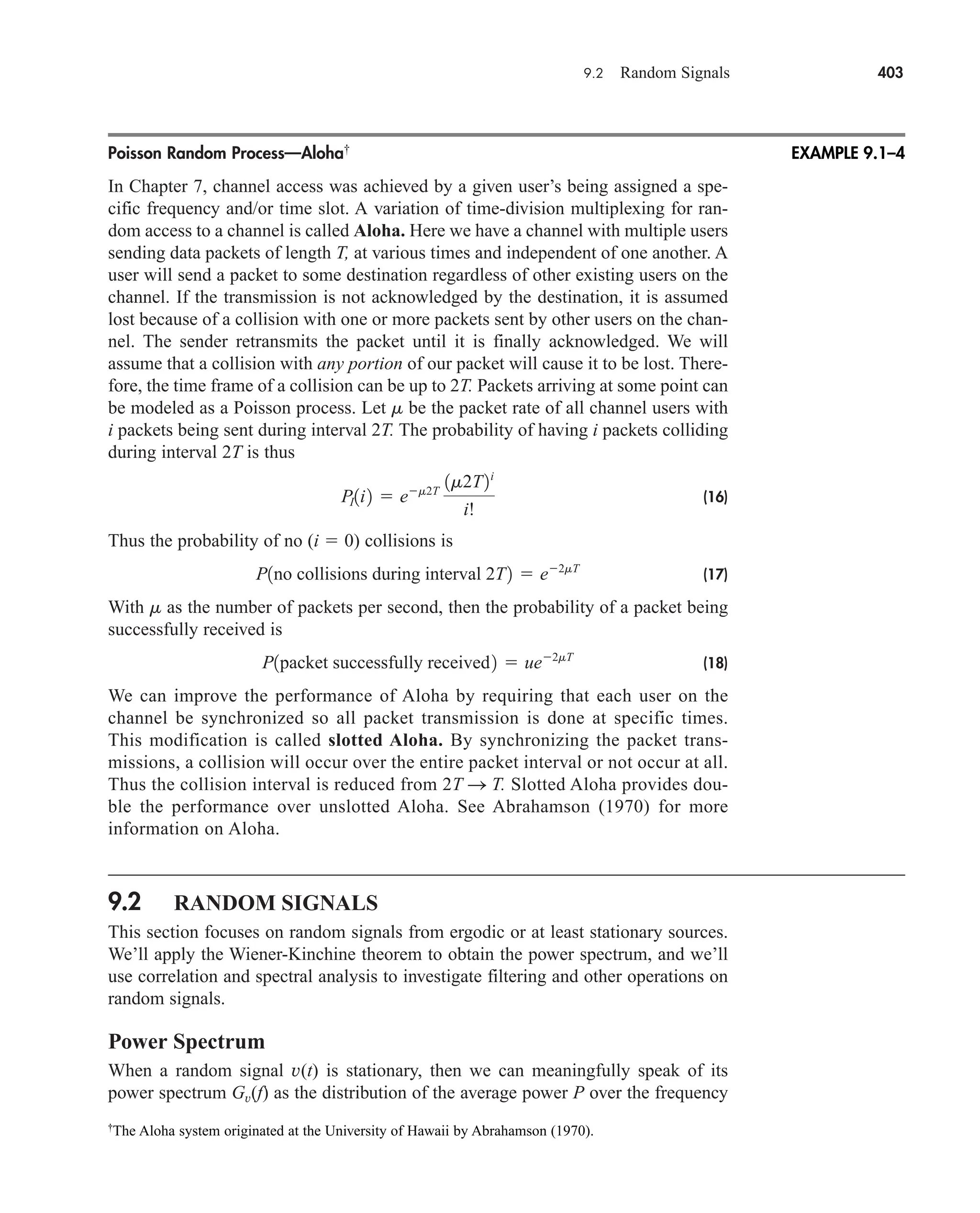
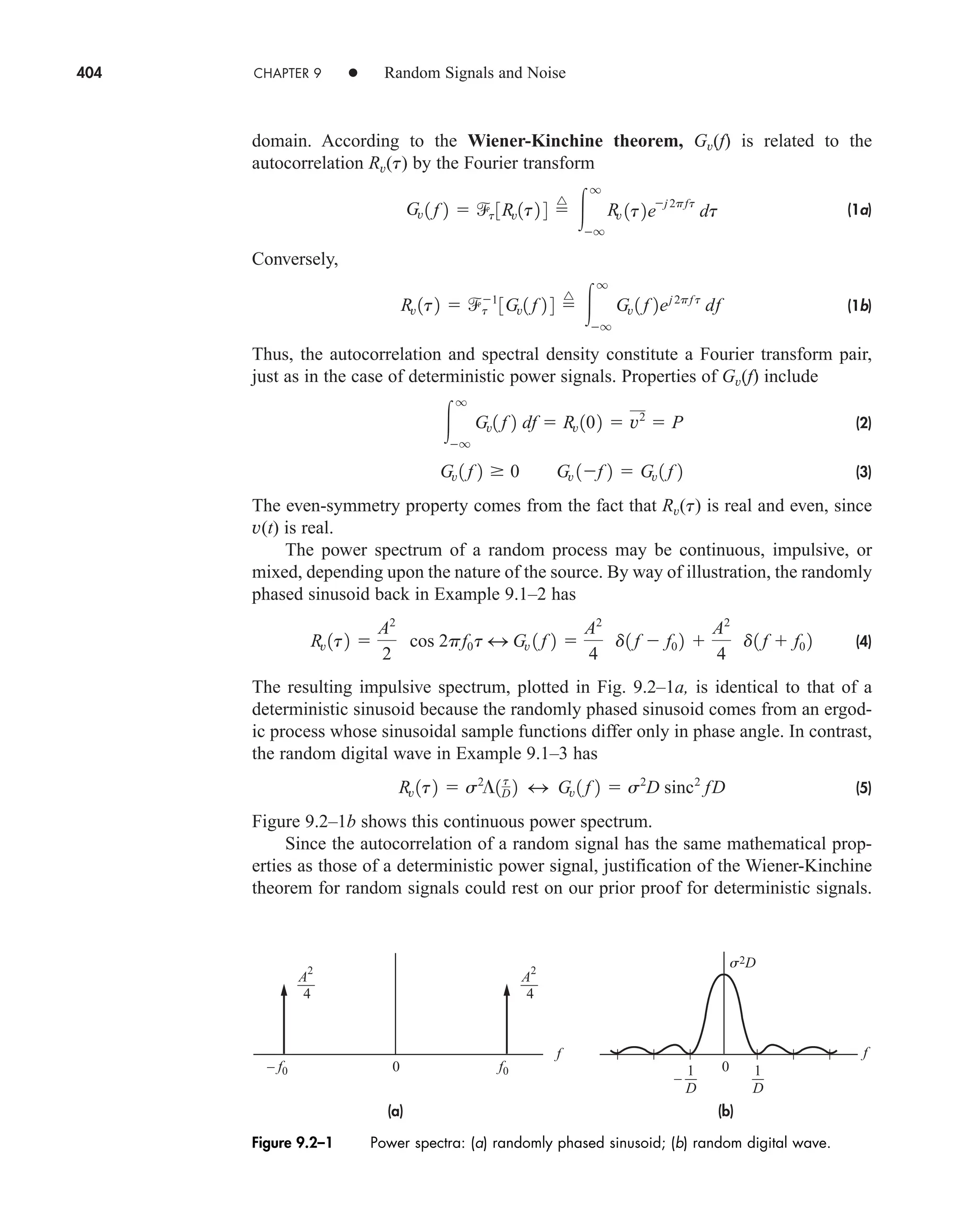
![9.2 Random Signals 405
However, an independent derivation based on physical reasoning provides addition-
al insight and a useful alternative definition of power spectrum.
Consider the finite-duration or truncated random signal
Since each truncated sample function has finite energy, we can introduce the
Fourier transform
(6)
Then VT(f,si)2
is the energy spectral density of the truncated sample function vT(t,si).
Furthermore, drawing upon Rayleigh’s energy theorem in the form
the average power of v(t) becomes
Accordingly, we now define the power spectrum of v(t) as
(7)
which agrees with the properties in Eqs.(2) and (3).
Conceptually, Eq. (7) corresponds to the following steps: (1) calculate the ener-
gy spectral density of the truncated sample functions; (2) average over the ensemble;
(3) divide by T to obtain power; and (4) take the limit T S . Equation (7) provides
the basis for experimental spectra estimation. For if we observe a sample function
v(t,si) for a long time T, then we can estimate Gv(f) from
The spectral estimate is called the periodogram because it originated in the
search for periodicities in seismic records and similar experimental data.
Now, to complete our derivation of the Wiener-Kinchine theorem, we outline the
proof that Gv(f) in Eq. (7) equals T[Rv(t)]. First, we substitute Eq. (6) into
and interchange integration and expectation to get
E30V
T 1 f, s2 024
T2
T2
E3v1t2v1l2 4ejv1tl2
dt dl
E3 0VT1f, s2 02
4 E3VT1f, s2VT
*1f, s2 4
G
v1 f 2
Gv
1 f 2
1
T
ƒVT 1 f,si 2ƒ 2
Gv 1 f 2
^
lim
TSq
1
T
E3 ƒV
T 1 f, s2 ƒ 24
lim
TSq
Ec
1
T
q
q
ƒV
T 1 f, s2 ƒ 2
df d
q
q
lim
TSq
1
T
E3ƒV
T 1 f, s2 ƒ 24 df
P lim
TSq
T2
T2
E3v2
1t2 4 dt
T2
T2
v2
1t2 dt
q
q
vT
2
1t2 dt
q
q
0VT 1 f, s2 02
df
VT 1 f, s2
q
q
vT
1t2ejvt
dt
T2
T2
v1t2ejvt
dt
vT 1t2
^
e
v1t2 0t0 6 T2
0 0t0 7 T2
car80407_ch09_391-438.qxd 12/17/08 5:20 PM Page 405
Confirming Pages](https://image.slidesharecdn.com/communicationsystemsanintro-a-241115060943-61721fa8/75/Communication_Systems__An_Intro_-_A-_Bruce_Carlson_-pdf-427-2048.jpg)
![406 CHAPTER 9 • Random Signals and Noise
in which
Next, let t t l and m t so the double integration is performed over the region
of the tm plane shown in Fig. 9.2–2. Integrating with respect to m for the two cases
t 0 and t 0 then yields
Finally, since t t for t 0, we have
(8)
Therefore,
which confirms that Gv(f) t[Rv(t)].
Random Telegraph Wave
Figure 9.2–3a represents a sample function of a random telegraph wave. This signal
makes independent random shifts between two equally likely values, A and 0. The
number of shifts per unit time is governed by a Poisson distribution, with m being
the average shift rate.
We’ll find the power spectrum given the autocorrelation function
Rv1t2
A2
4
1e2m 0t 0
12
lim
TSq
1
T
E3 0V
T 1 f, s2 024
q
q
Rv 1t2ejvt
dt
E 3 0V
T 1 f, s2 024 T
T
T
a1
0t0
T
bRv1t2ejvt
dt
0
T
Rv 1t2ejvt
1T t2dt
T
0
Rv 1t2ejvt
1T t2dt
E3 0V
T 1 f, s2 024
0
T
Rv1t2ejvt
a
tT2
T2
dmbdt
T
0
Rv 1t2ejvt
a
T2
tT2
dmbdt
E3v1t2v1l2 4 Rv1t, l2 Rv 1t l2
Figure 9.2–2 Integration region in the tm plane.
T/2
–T/2
m = t + T/2
m = t – T/2
–T T
m
t
0
EXAMPLE 9.2–1
car80407_ch09_391-438.qxd 12/22/08 2:44 PM Page 406
Rev. Confirming Pages](https://image.slidesharecdn.com/communicationsystemsanintro-a-241115060943-61721fa8/75/Communication_Systems__An_Intro_-_A-_Bruce_Carlson_-pdf-428-2048.jpg)
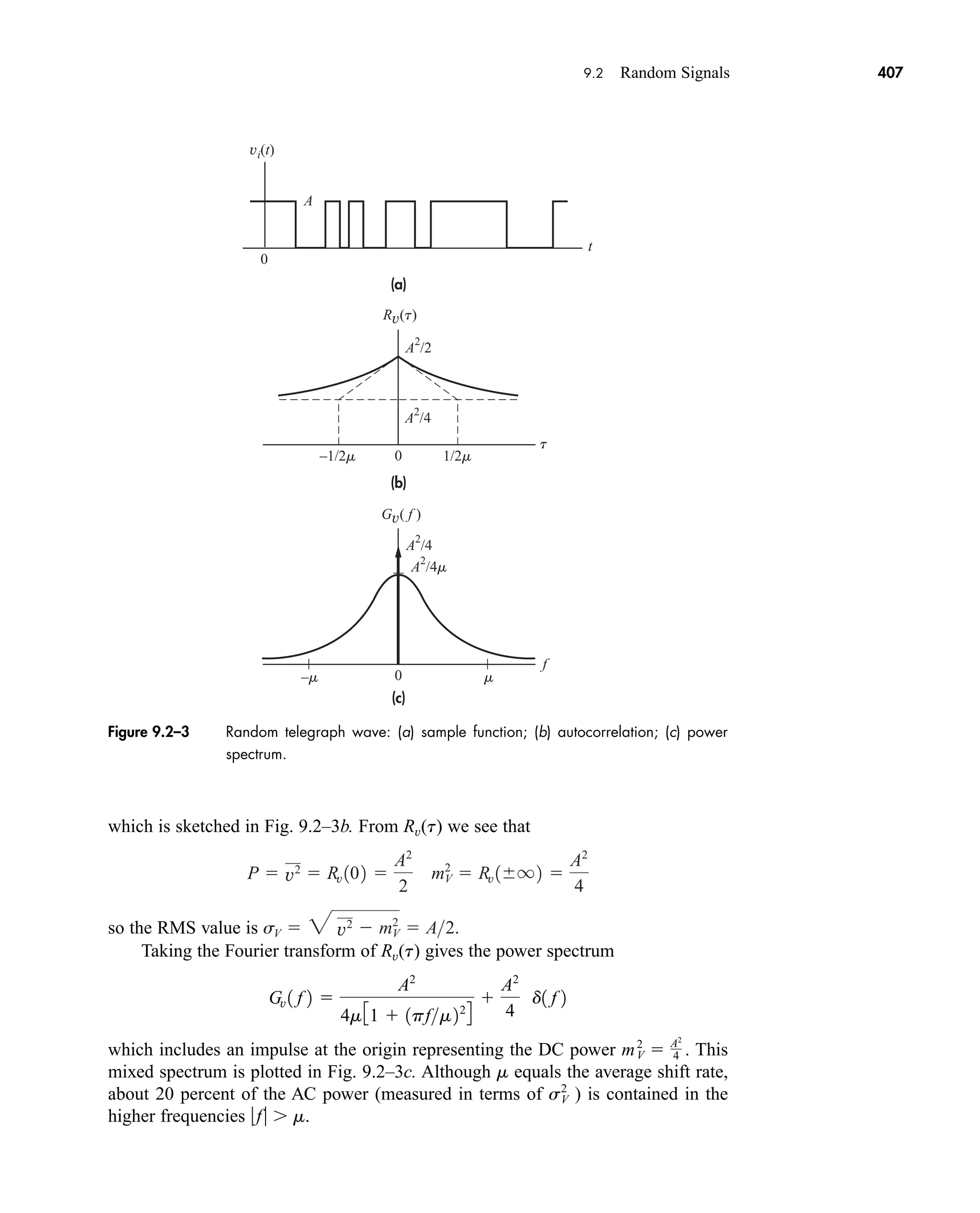
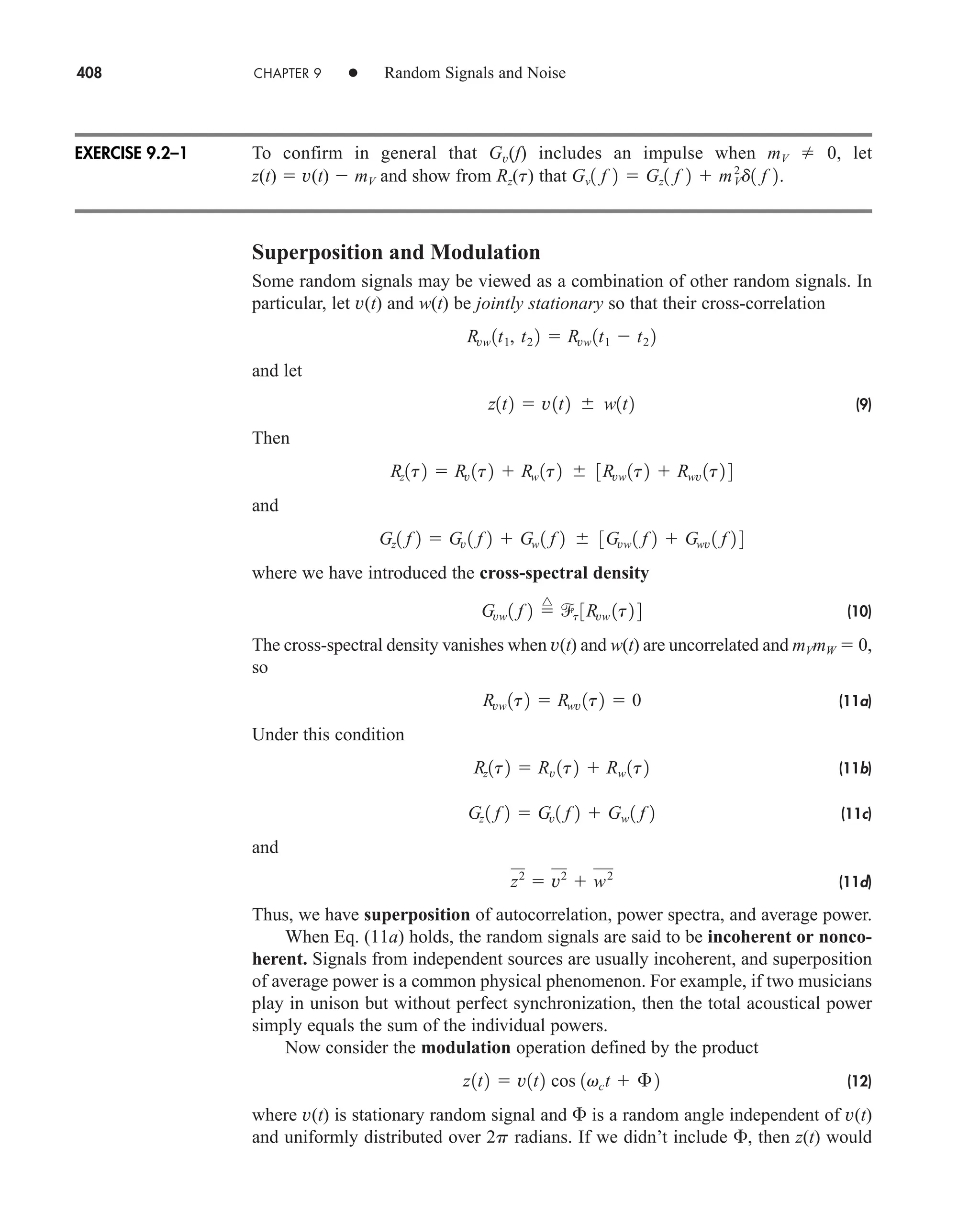
![9.2 Random Signals 409
be nonstationary; including merely recognizes the arbitrary choice of the time ori-
gin when v(t) and cos vct come from independent sources.
Since modulation is a time-varying process, we must determine Rz(t) from
Rz(t1, t2) E[z(t1)z(t2)] by taking the joint expectation with respect to both v and .
After trigonometric expansion we get
Thus, with t t1 t2,
(13a)
and Fourier transformation yields
(13b)
Not surprisingly, modulation translates the power spectrum of v(t) up and down by
fc units.
Modulation is a special case of the product operation
(14)
If v(t) and w(t) are independent and jointly stationary, then
(15a)
and
(15b)
which follows from the convolution theorem.
Derive Eq. (13b) from Eq. (15b) by making a judicious choice for w(t).
Filtered Random Signals
Figure 9.2–4 represents a random signal x(t) applied to the input of a filter (or any
LTI system) having transfer function H(f) and impulse response h(t). The resulting
output signal is given by the convolution
(16)
Since convolution is a linear operation, a gaussian input produces a gaussian output
whose properties are completely described by mY and Ry(t). These output statistics
can be found from H(f) or h(t), and they will be useful even in the nongaussian case.
y1t2
q
q
h1l2x1t l2dl
Gz1 f 2 Gv1 f 2*Gw1 f 2
Rz1t2 Rv1t2Rw 1t2
z1t2 v1t2w1t2
Gz1 f 2 1
4 3Gv1 f fc 2 Gv1 f fc 2 4
Rz1t2 1
2Rv1t2 cos 2pfct
1
2Rv1t1, t2 2 cos vc 1t1 t2 2
Rz1t1, t2 2 1
2 E 3v1t1 2v1t2 2 45cos vc1t1 t2 2 E3cos 1vct1 vct2 2£ 2 46
EXERCISE 9.2–2
car80407_ch09_391-438.qxd 12/17/08 5:21 PM Page 409
Confirming Pages](https://image.slidesharecdn.com/communicationsystemsanintro-a-241115060943-61721fa8/75/Communication_Systems__An_Intro_-_A-_Bruce_Carlson_-pdf-431-2048.jpg)
![410 CHAPTER 9 • Random Signals and Noise
We’ll assume that h(t) is real, so both x(t) and y(t) are real. We’ll also assume
that x(t) is a stationary power signal and that the system is stable. Under these con-
ditions, y(t) will be a stationary power signal and the output-input cross-correlation
is a convolution with the impulse response, namely,
(17a)
The proof of this relation starts with Ryx(t1,t2) E[y(t1)x(t2)]. Inserting y(t1) from
Eq. (16) and exchanging the order of operations yields
Then, since x(t) is stationary,
Finally, letting t2 t1 t,
so Ryx(t) h(t)*Rx(t). Proceeding in the same fashion, the output autocorrelation is
found to be
(17b)
which also establishes the fact that y(t) is at least wide-sense stationary.
From Eq. (17b), it follows that the power spectra are related by
(18)
Consequently,
(19a)
(19b)
Furthermore, the mean value of the output is
(20)
mY c
q
q
h1l2dldmX H102mX
y2
Ry 102
q
q
0H1 f 202
Gx1 f 2 df
Ry1t2 t
1
3 0H1 f 202
Gx1 f 2 4
Gy1 f 2 0H1 f 202
Gx1 f 2
Ry1t2 h1t2*Ryx 1t2 h1t2*h1t2*Rx 1t2
Ryx 1t1, t1 t2 Ryx 1t2
q
q
h1l2Rx1t l2 dl
E3x1t1 l2x1t2 2 4 Rx 1t1 l, t2 2 Rx 1t1 l t2 2
Ryx 1t1, t2 2
q
q
h1l2E3x1t1 l2x1t2 2 4dl
Ryx 1t2 h1t2*Rx 1t2
h(t)
x(t)
Rx(t)
Gx( f )
y(t)
Ry(t)
Gy( f )
H( f )
Figure 9.2–4 Random signal applied to a filter.
car80407_ch09_391-438.qxd 12/17/08 5:21 PM Page 410
Confirming Pages](https://image.slidesharecdn.com/communicationsystemsanintro-a-241115060943-61721fa8/75/Communication_Systems__An_Intro_-_A-_Bruce_Carlson_-pdf-432-2048.jpg)
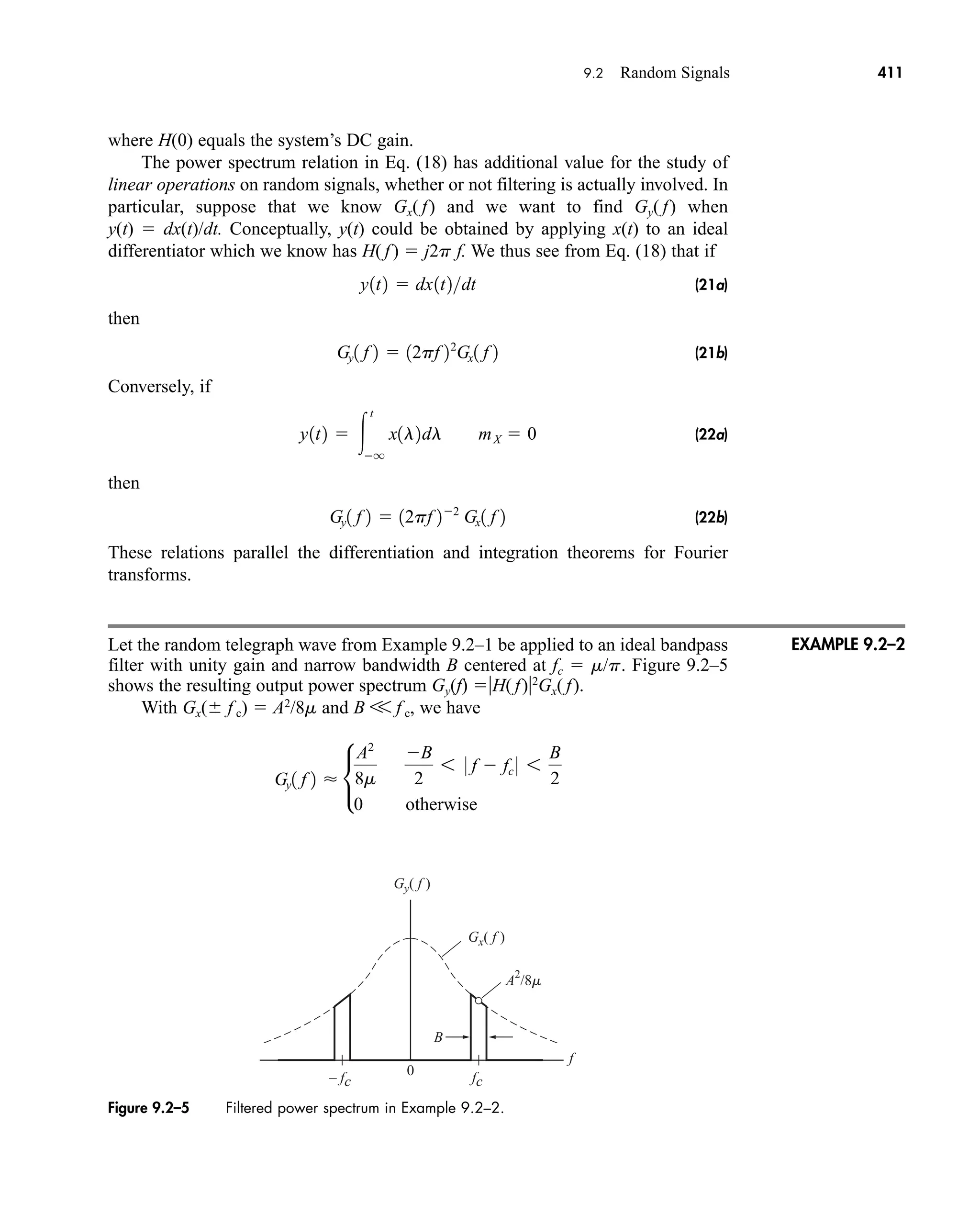
![412 CHAPTER 9 • Random Signals and Noise
and the output power equals the area under Gy(f), namely
whereas Moreover, since H(0) 0, we know from Eq. (20) that mY 0
even though mX A/2. Note that we obtained these results without the added labor
of finding Ry(t).
Hilbert Transform of a Random Signal
The Hilbert transform was previously defined as the output of a quadrature
phase-shifting filter having
Since HQ( f)2
1, we now conclude that if x(t) is a random signal and y(t)
then
Thus, Hilbert transformation does not alter the values of mX or
However, from Eq. (17a),
where stand for the Hilbert transform of Rx(t). It can also be shown that
We’ll apply these results in the next chapter.
Let the random digital wave described by Eq. (5) be applied to a first-order LPF with
H( f) [1 j( f/B)]1
and B V 1/D. Obtain approximate expressions for Gy( f)
and Ry(t).
9.3 NOISE
Unwanted electric signals come from a variety of sources, generally classified as either
human interference or naturally occurring noise. Human interference is produced by
other communication systems, ignition and commutator sparking, AC hum, and so
forth. Natural noise-generating phenomena include atmospheric disturbances, extra-
terrestrial radiation, and random electron motion. By careful engineering, the effects
Rxx̂1t2 R̂x1t2
R̂x 1t2
Rx̂x 1t2 hQ1t2*Rx1t2 R̂
x 1t2
x2
.
Gx̂ 1 f 2 Gx 1 f 2 Rx̂ 1t2 t
1
3Gx̂ 1 f 2 4 Rx 1t2
x̂1t2,
hQ 1t2
1
pt
HQ 1 f 2 j sgn f
x̂1t2
x2
A2
2.
y2
2B a
A2
8m
b
A2
B
4m
V
A2
4p
EXAMPLE 9.2–3
EXERCISE 9.2–3
car80407_ch09_391-438.qxd 12/17/08 5:21 PM Page 412
Confirming Pages](https://image.slidesharecdn.com/communicationsystemsanintro-a-241115060943-61721fa8/75/Communication_Systems__An_Intro_-_A-_Bruce_Carlson_-pdf-434-2048.jpg)
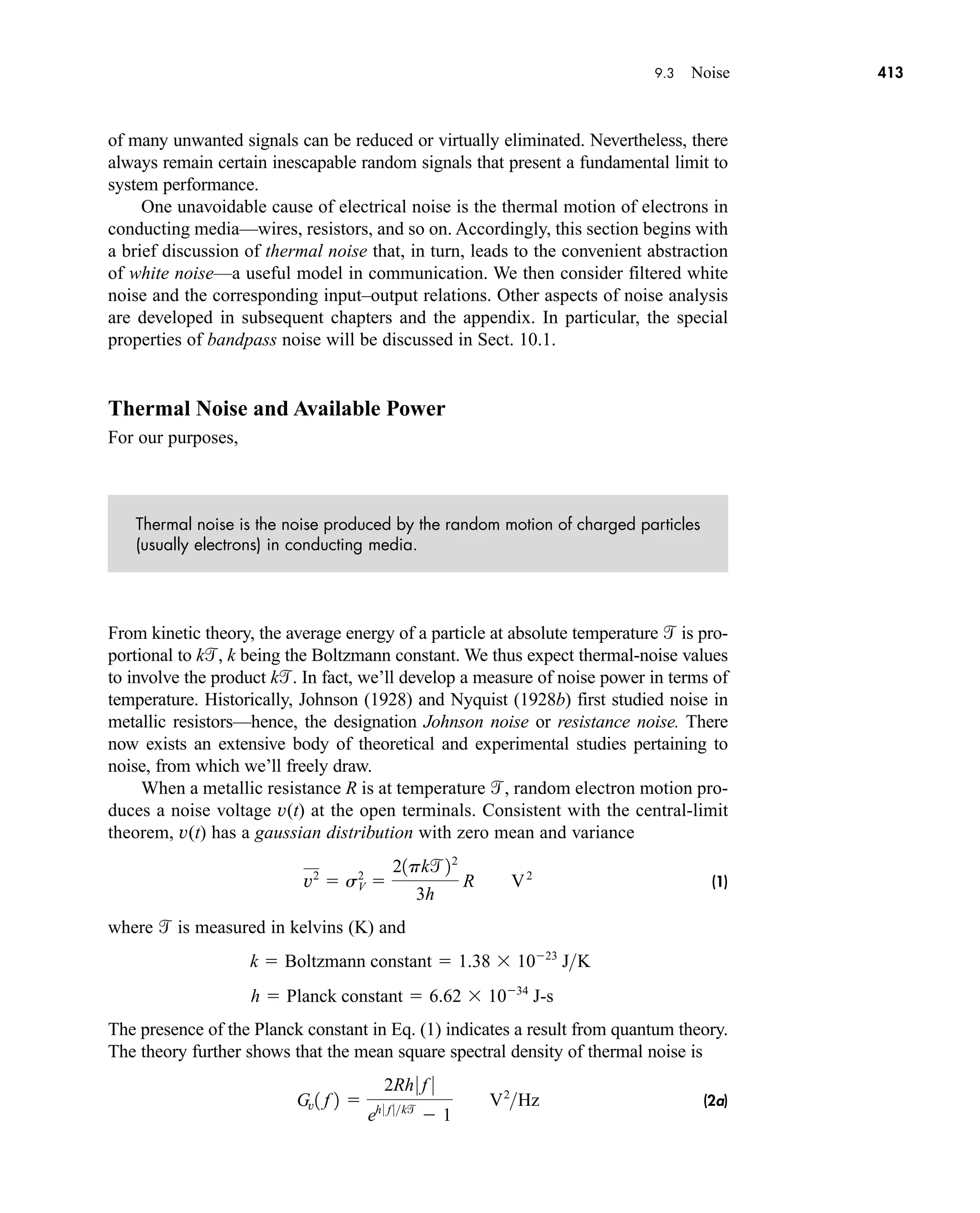
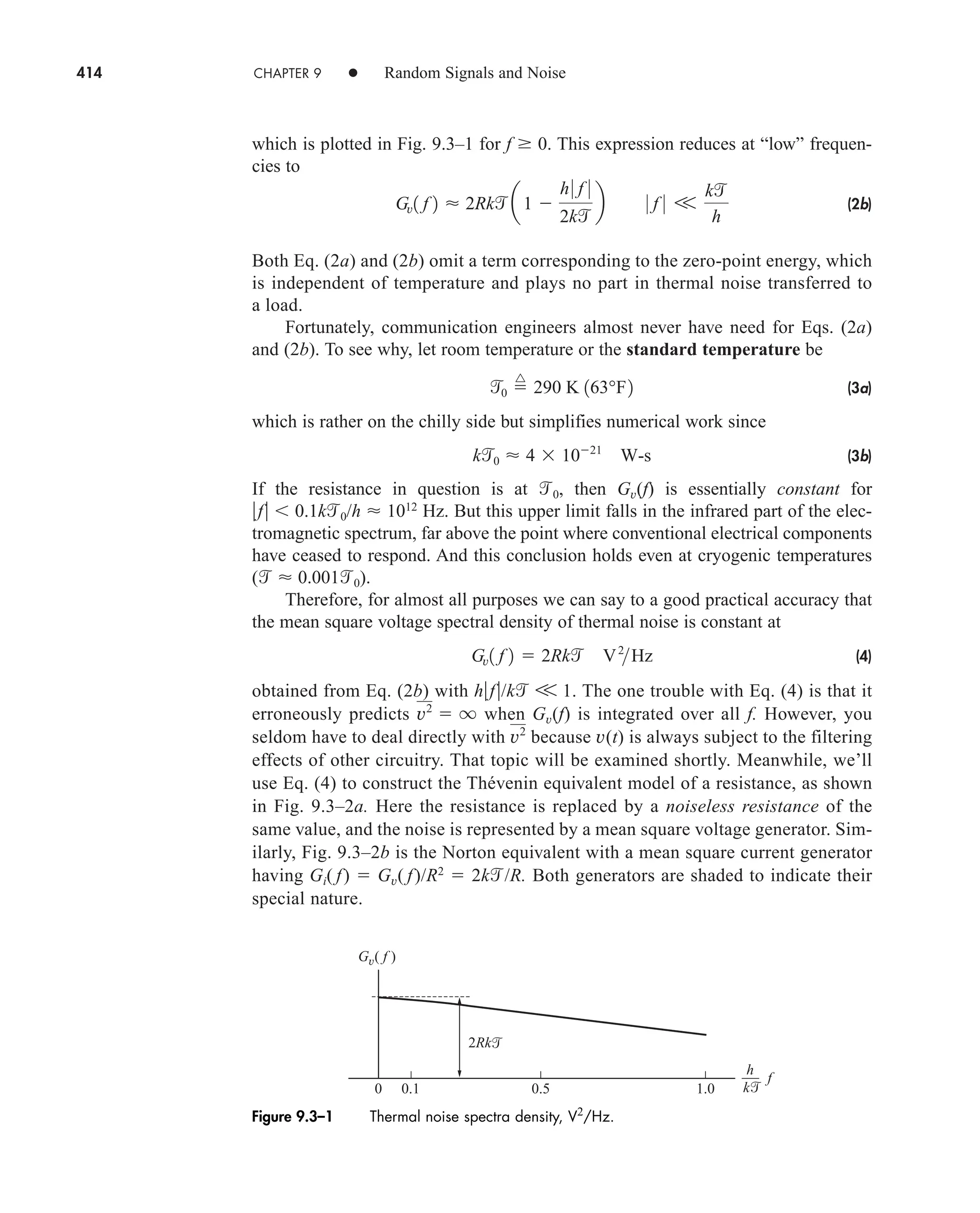
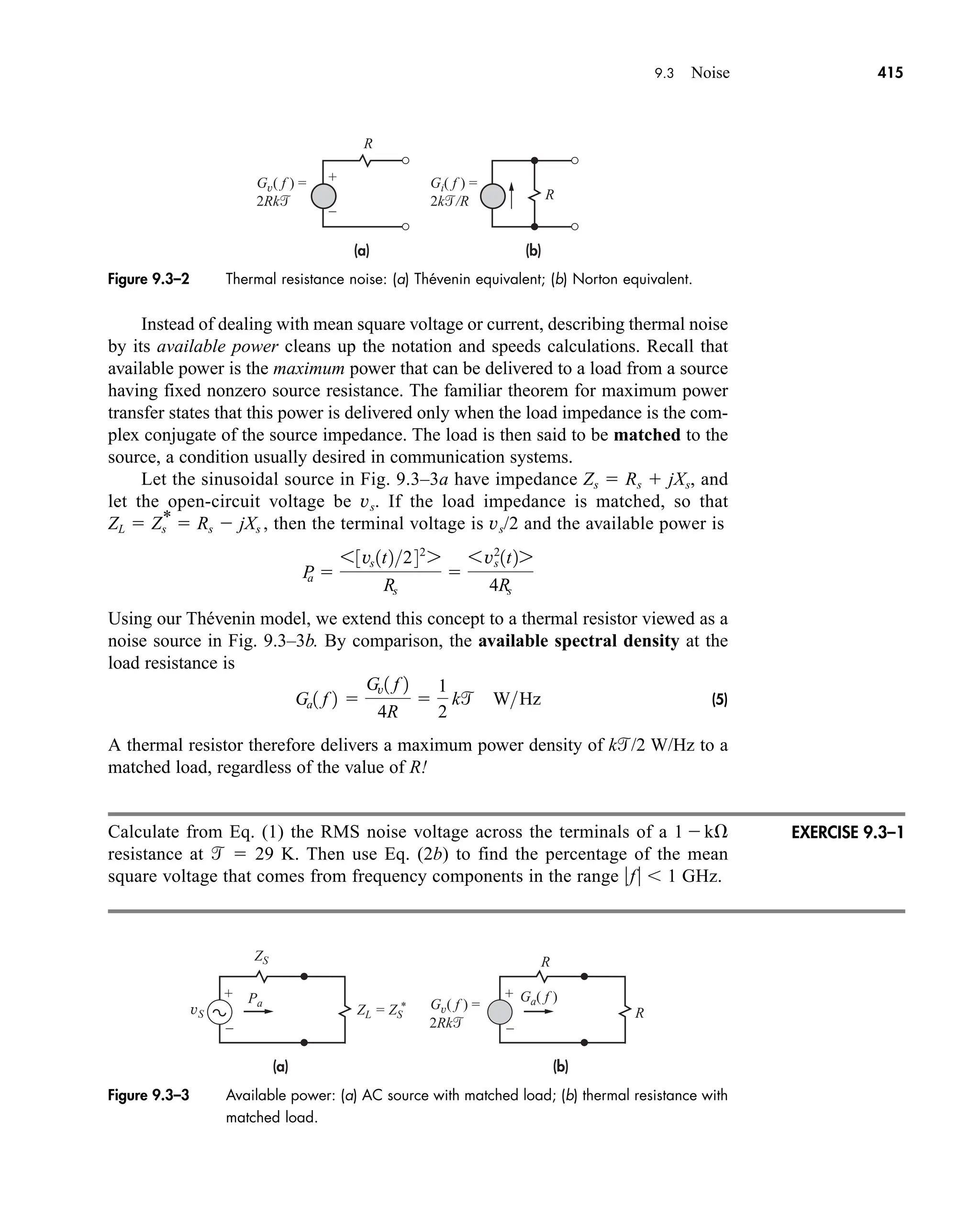
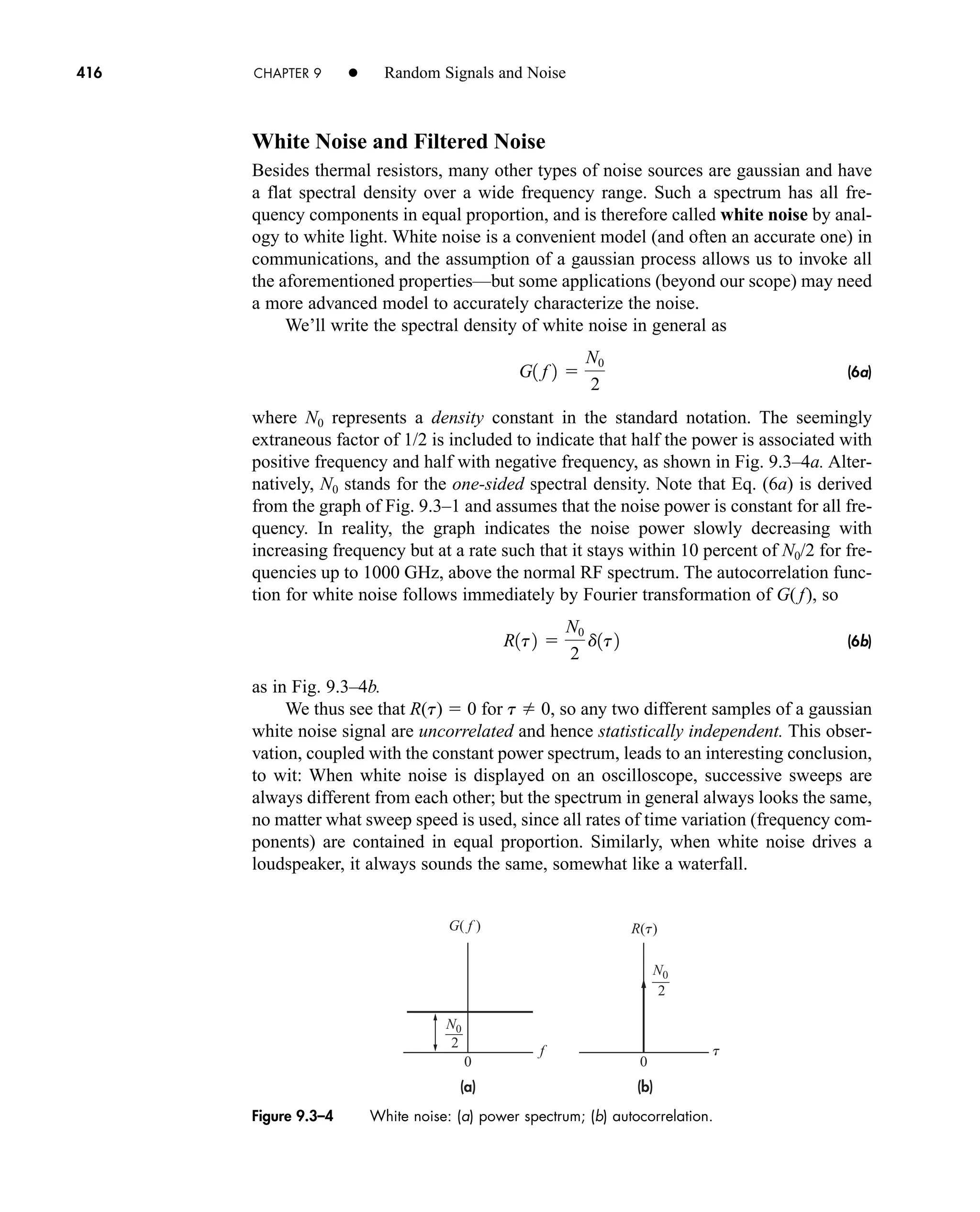
![418 CHAPTER 9 • Random Signals and Noise
(10a)
which are plotted in Fig. 9.3–5. Besides the spectral shaping, we see that lowpass fil-
tering causes the output noise to be correlated over time intervals of about 1/2B. We
also see that
(10b)
so the output power is directly proportional to the filter’s bandwidth.
Thermal Noise in an RC Network
To pull together several of the topics so far, consider the RC network in Fig. 9.3–6a
with the resistor at temperature . Replacing this thermal resistor with its Thévenin
model leads to Fig. 9.3–6b, a white-noise mean square voltage source with
Gx( f) 2Rk V2
/Hz applied to a noiseless RC LPF. Since H( f)2
[1 ( f/B)2
]1,
the output spectral density is
(11a)
The inverse transform then yields
(11b)
Ry1t2 2RkpBe2pB0 t 0
k
C
e0t 0RC
Gy1 f 2 0H1 f 2 0 2
Gx1 f 2
2Rk
1 1 fB22 B
1
2pRC
y2
N0B
Gy1 f 2
N0
2
ß a
f
2B
b Ry 1t2 N0B sinc 2Bt
Figure 9.3–5 White noise passed by an ideal LPF: (a) power spectrum; (b) autocorrelation.
(a) (b)
–B B
f
Gy( f )
0
2
N0
N0B
2B
1
–
2B
1
t
0
Ry(t)
(a) (b)
Gx( f ) =
y2 = k/C
2Rk
C C
R
R
+
–
Figure 9.3–6 (a) RC network with resistance noise; (b) noise equivalent model.
EXAMPLE 9.3–1
car80407_ch09_391-438.qxd 12/17/08 5:21 PM Page 418
Confirming Pages](https://image.slidesharecdn.com/communicationsystemsanintro-a-241115060943-61721fa8/75/Communication_Systems__An_Intro_-_A-_Bruce_Carlson_-pdf-440-2048.jpg)
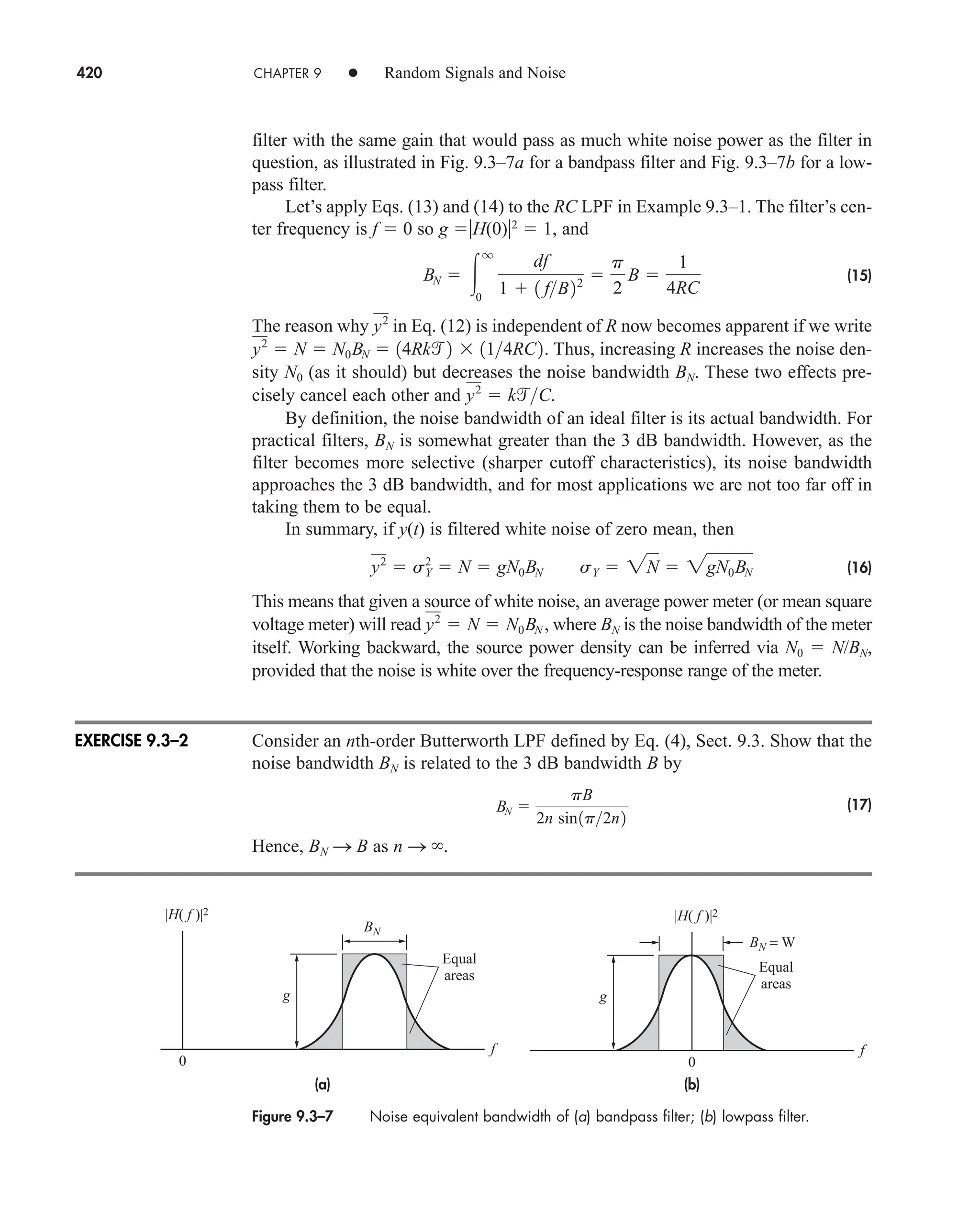
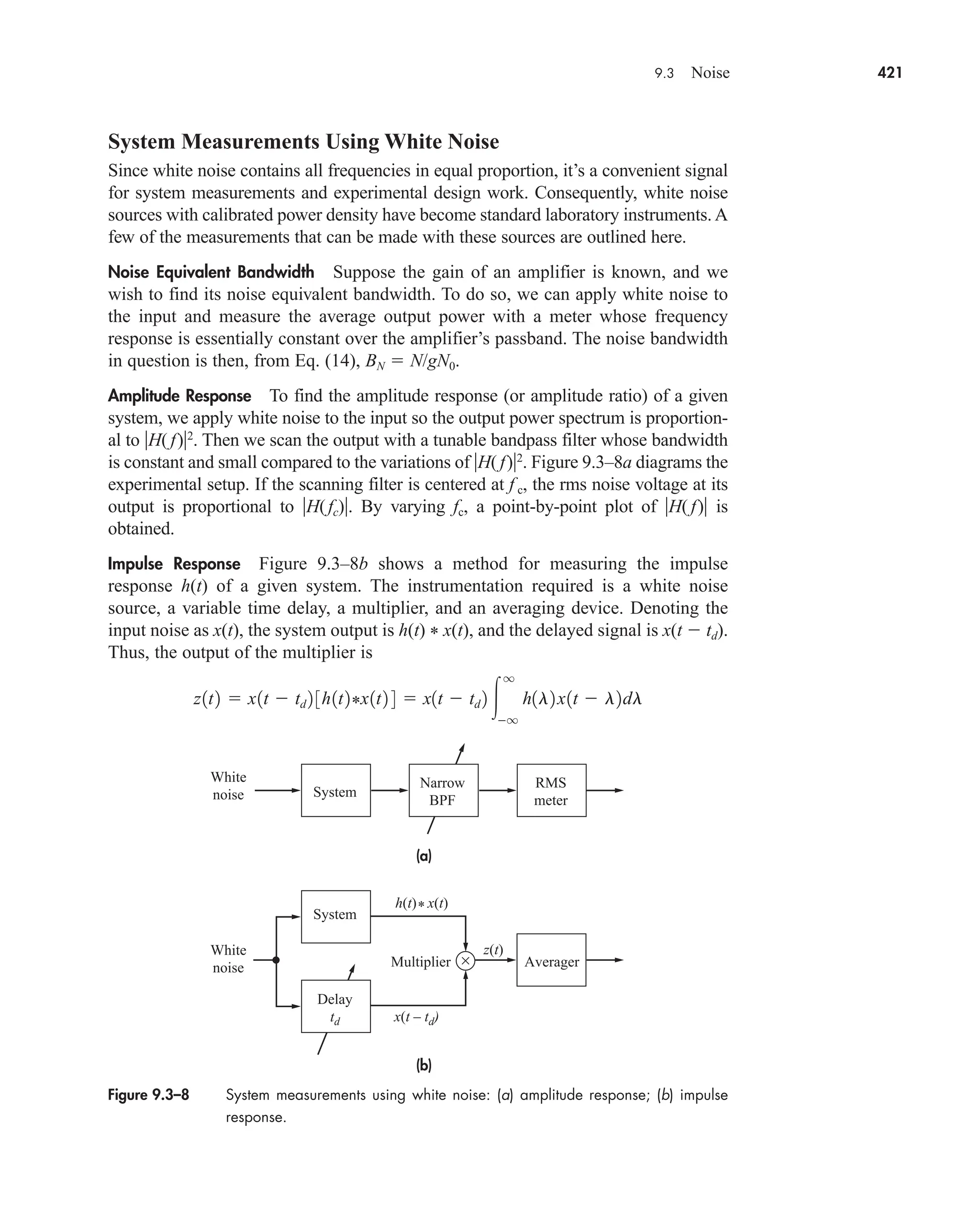
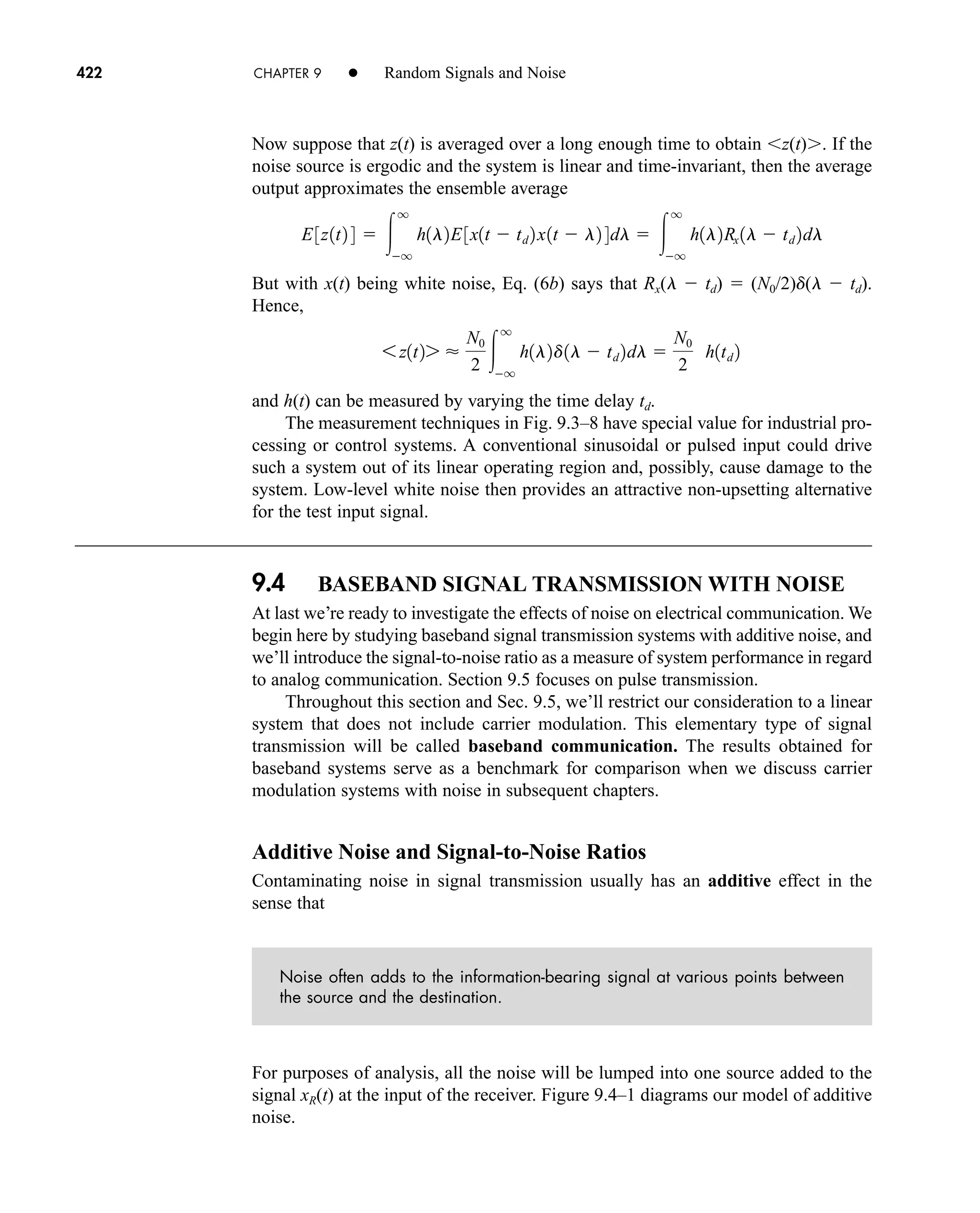
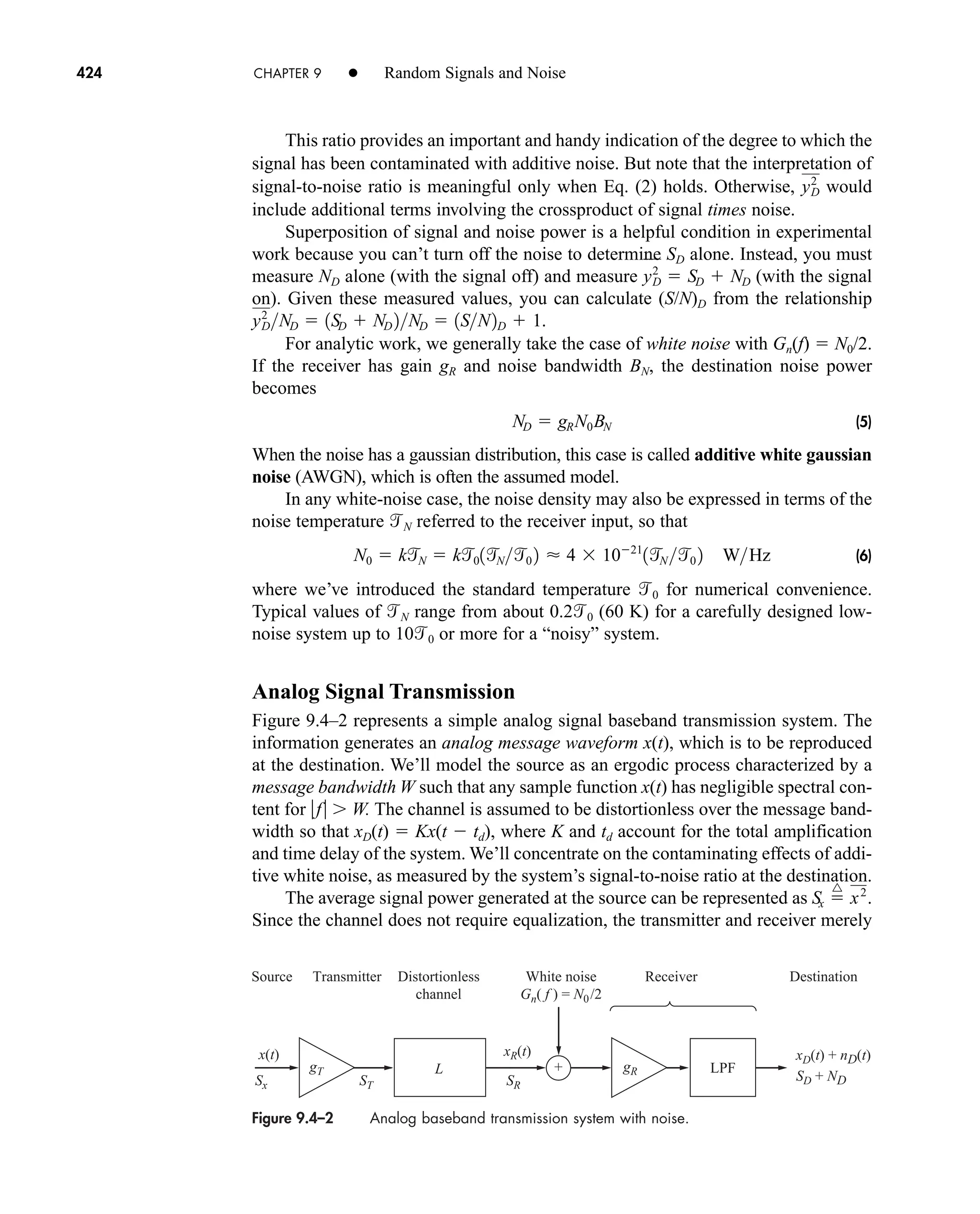
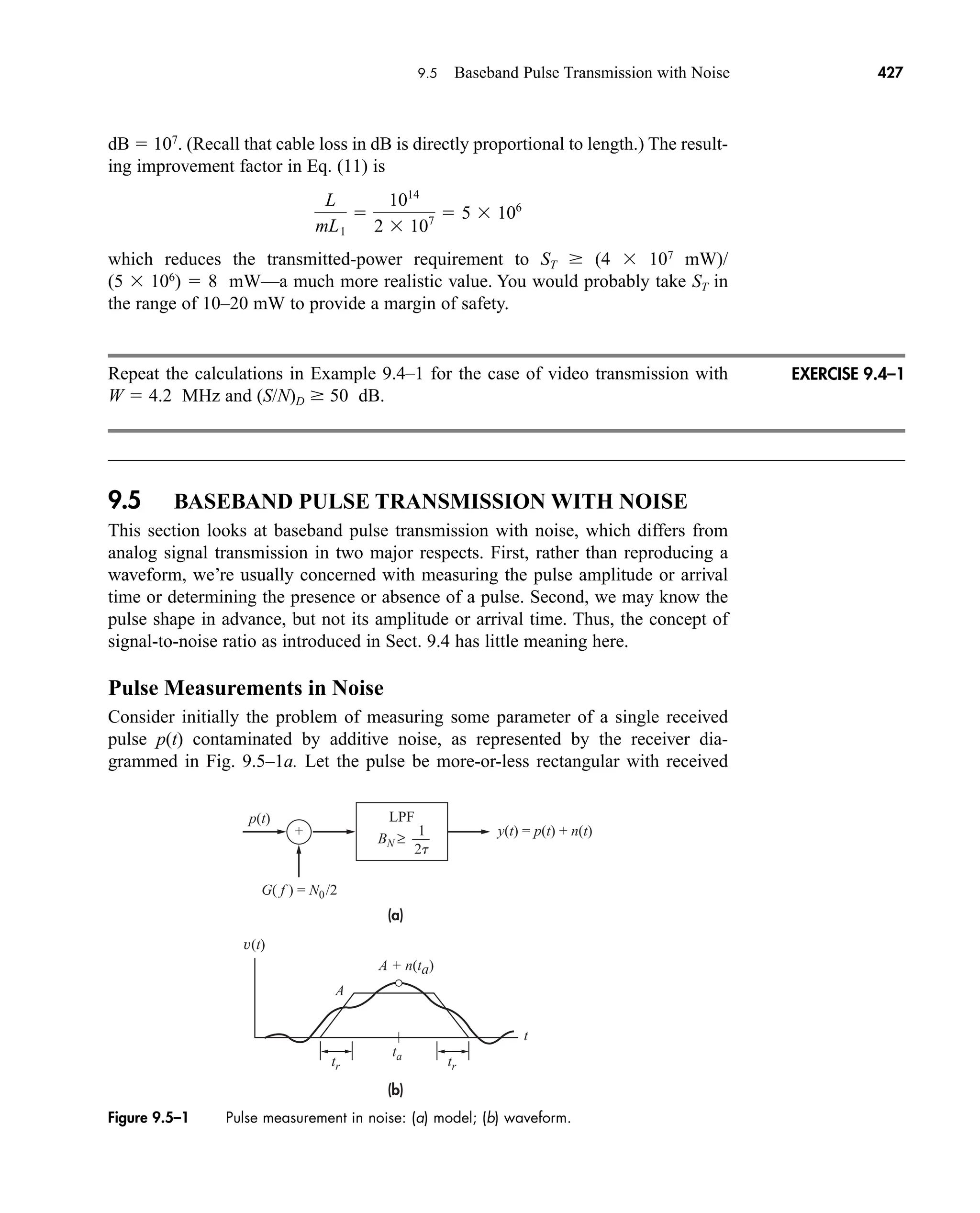
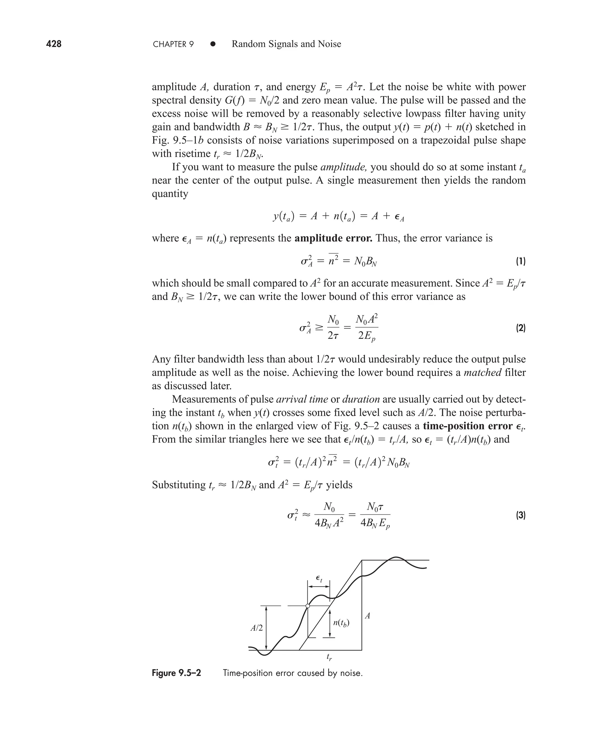
![9.5 Baseband Pulse Transmission with Noise 429
which implies that we can make st arbitrarily small by letting BN S so that tr S 0.
But the received pulse actually has a nonzero risetime determined by the
transmission bandwidth BT. Hence,
(4)
and the lower bound is obtained with filter bandwidth BN BT—in contrast to the
lower bound on sA obtained with BN 1/2t.
Suppose a 10-ms pulse is transmitted on a channel having BT 800 kHz and
N0 Ep/50. Calculate sA/A and st/t when: (a) BN 1/2t; (b) BN Bt.
Pulse Detection and Matched Filters
When we know the pulse shape, we can design optimum receiving filters for
detecting pulses buried in additive noise of almost any known spectral density
Gn(f). Such optimum filters, called matched filters, have extensive applications in
digital communication, radar systems, and the like.
Figure 9.5–3a will be our model for pulse detection. The received pulse has
known shape p(t) but unknown amplitude Ap and arrival time t0, so the received
signal is
(5a)
Thus, the Fourier transform of xR(t) will be
(5b)
where P(f) [p(t)]. The total received pulse energy is
(5c)
Ep
q
q
0XR1 f 2 02
df Ap
2
q
q
0P1 f 2 02
df
XR1 f 2 ApP1 f 2ejvt0
xR1t2 Ap p1t t0 2
s2
t
N0
4BT A2
N0t
4BT Ep
EXERCISE 9.5–1
Figure 9.5–3 Pulse detection in noise: (a) model; (b) filtered output.
(b)
(a)
Gn( f )
xR(t) =
App(t – t0)
t0 + td
A + n
y(t)
y(t)
H( f )
+ t
car80407_ch09_391-438.qxd 12/22/08 2:44 PM Page 429
Rev. Confirming Pages](https://image.slidesharecdn.com/communicationsystemsanintro-a-241115060943-61721fa8/75/Communication_Systems__An_Intro_-_A-_Bruce_Carlson_-pdf-451-2048.jpg)
![9.6 Questions and Problems 433
8. Explain why in an antenna-transmission line-receiver system the best SNR
performance requires that the preamp be located nearest to the antenna.
9. Give a real-world example of why amplifying a signal in the latter stages of the
receiver (e.g., the IF or AF stages) does not necessarily improve reception quality.
10. Can an amplifier at the receiver’s input improve the signal-to-noise ratio? Why
or why not?
11. Give an analogy to an Aloha system.
12. Many instrumentation systems suffer when the sensor amplifier suffers from 1/f
noise. How can we mitigate against this?
13. Why would thermal noise have a gaussian distribution?
Problems
9.1–1* The random variable X has a uniform distribution over 0 x 2. Find
Rv(t1, t2), and for the random process v(t) 6eXt
.
9.1–2 Do Prob. 9.1–1 with v(t) 6 cos Xt.
9.1–3 Let X and Y be independent RVs. Given that X has a uniform distribution
over 1 x 1 and that and find Rv(t1, t2), and
for the random process v(t) (Y 3Xt)t.
9.1–4 Do Prob. 9.1–3 with v(t) YeXt
.
9.1–5 Do Prob. 9.1–3 with v(t) Y cos Xt.
9.1–6‡ Let v(t) A cos (2pFt ) where A is a constant and F and are
RVs. If has a uniform distribution over 2p radians and F has an arbi-
trary PDF pF(f), show that
Also find and
9.1–7* Let X and Y be independent RVs, both having zero mean and variance s2
.
Find the crosscorrelation function of the random processes
9.1–8 Consider the process v(t) defined in Prob. 9.1–7. (a) Find and
Rv(t1, t2) to confirm that this process is wide-sense stationary. (b) Show,
from E[v2
(t)] and that the process is not ergodic.
9.1–9 Let v(t) A cos (v 0t ), where A and are independent RVs and
has a uniform distribution over 2p radians. (a) Find and Rv(t1, t2) to
v1t2
6vi
2
1t27,
v1t2
w1t2 Y cos v0t X sin v0t
v1t2 X cos v0t Y sin v0t
v2
1t2 .
v1t2
Rv 1t1, t2 2
A2
2
q
q
cos 2pl1t1 t2 2pF 1l2 dl
v2
1t2
v1t2,
Y2
6,
Y 2
v2
1t2
v1t2 ,
car80407_ch09_391-438.qxd 12/17/08 5:21 PM Page 433
Confirming Pages](https://image.slidesharecdn.com/communicationsystemsanintro-a-241115060943-61721fa8/75/Communication_Systems__An_Intro_-_A-_Bruce_Carlson_-pdf-455-2048.jpg)
![434 CHAPTER 9 • Random Signals and Noise
confirm that this process is wide-sense stationary. (b) Show, from
E[v2
(t)] and that the process is not ergodic.
9.1–10* Let z(t) v(t) v(t T), where v(t) is a stationary nonperiodic process
and T is a constant. Find the mean and variance of z(t) in terms of Rv(t).
9.1–11 Do Prob. 9.1–10 with z(t) v(t) v(t T).
9.1–12 Let v(t) and w(t) be two independent processes. Show that they will be
uncorrelated.
9.2–1* A certain random signal has 9. Find the power spec-
trum and determine the signal’s dc value, average power, and rms value.
9.2–2 Do Prob. 9.2–1 with Rv(t) 32sinc2
8t 4cos 8t.
9.2–3 Consider the signal defined in Prob. 9.1–6. Show that Gv( f)
(A2
/4)[pF( f) pF(f)]. Then simplify this expression for the case when
F f0, where f0 is a constant.
9.2–4 Consider the spectral estimate Use Eq. (8) to show
that What happens in the limit as
T S ?
9.2–5‡
Let v(t) be a randomly phased sinusoid. Show that Eq. (7) yields Gv(f)
in Eq. (4).
9.2–6 Modify Eqs. (11b)–(11d), for the case when v(t) and w(t) are independ-
ent stationary signals with mVmW 0. Show from your results that
Rz ( ) (mV mW)2
and that
9.2–7 Let v(t) and w(t) be jointly stationary, so that Rvw(t1, t2) Rvw(t1 t2).
Show that
What’s the corresponding relationship between the cross-spectral densities?
9.2–8 Let z(t) v(t) v(t T), where v(t) is a stationary random signal and
T is a constant. Start with Rz(t1, t2) to find Rz(t) and Gz( f) in terms of
Rv(t) and Gv( f).
9.2–9 Do Prob. 9.2–8 with z(t) v(t) v(t T).
9.2–10 Let z(t) A cos (2pf1t 1) cos (2pf2t 2), where A, f1, and f2
are constants, and 1 and 2 are independent RVs, both uniformly dis-
tributed over 2p radians. Find Gz( f) and simplify it for the case f1 f2.
9.2–11 Confirm that Ry(t) h(t) * Ryx(t).
9.2–12* Let y(t) dx(t)/dt. Find R y(t) and Ryx(t) in terms of Rx(t) by taking the
inverse transforms of Gy( f) and Gyx( f).
9.2–13 Let y(t) x(t) ax(t T), where a and T are constants. Obtain expres-
sions for Gy( f) and Ry(t).
Rwv 1t2 Rvw1t2
z2
7 0.
E 3Gv
1 f 2 4 1T sinc2
f T2 * Gv 1 f 2
G
v1 f 2 0VT 1 f, s2 02
T.
Rv1t2 16e18t22
6vi
2
1t27,
car80407_ch09_391-438.qxd 12/22/08 2:44 PM Page 434
Rev. Confirming Pages](https://image.slidesharecdn.com/communicationsystemsanintro-a-241115060943-61721fa8/75/Communication_Systems__An_Intro_-_A-_Bruce_Carlson_-pdf-456-2048.jpg)


![9.6 Questions and Problems 437
9.4–4 Consider an AWGN baseband transmission system with W 10 kHz.
Express (S/N)D in a form like Eq. (8), when the receiving filter is: (a) a
first-order LPF with B 15 kHz; (b) a second-order Butterworth LPF
with B 12 kHz.
9.4–5 Consider a baseband system with (S/D)D 30 dB, W 3 kHz,
ST 100 W. What is new value of W if the system were changed so that
(S/N)D 10 dB, and W 100 Hz?
9.4–6 Consider a baseband system carrying a voice messages with a given
(S/N)D, and W over a wireless link at a carrier frequency fc. Let’s assume
the noise figure of the receiver and channel cannot be changed. Describe
all possible means to increase the (S/N)D.
9.4–7* Consider a baseband transmission system with additive white noise and
a distorting channel having HC(f)2
1/{L[1 (f/W)2
]}. The distortion
is equalized by a receiving filter with HR(f)2
[K/HC(f)]2
(f/2W).
Obtain an expression for (S/N)D in the form like Eq. (10).
9.4–8 Do Prob. 9.4–7 with HC(f)2
1/{L[1 (2f/W)4
]}.
9.4–9 A baseband signal with W 5 kHz is transmitted 40 km via a cable
whose loss is a 3 dB/km. The receiver has N 100. (a) Find ST
needed to get (S/N)D 60 dB. (b) Repeat the calculation assuming a
repeater at the midpoint.
9.4–10 A cable transmission system with L 240 dB has m 6 equal-length
repeater sections and (S/N)D 30 dB. Find the new value of (S/N)D if
(a) m is increased to 12; (b) m is decreased to 4.
9.4–11* The cable for a 400 km repeater system has a 0.5 dB/km. Find the
minimum number of equal-length repeater sections needed to get
(S/N)D 30 dB if ST/N0W 80 dB.
9.4–12 If all other parameters of a cable transmission system are fixed, show
that the number of equal-length repeater sections that maximizes (S/N)D
is m 0.23L dB.
9.4–13 Given a cable system with a 2 dB/km, l 3000 km, (S/D)D 30 dB,
N 50, and W 3 kHz. What is the minimum number of repeater
links to enable ST 100 W?
9.4–14‡
The open-circuit signal voltage output of an oscillator is A cos 2pf0t. The
oscillator has a noiseless source resistance R and internally generated
thermal noise at temperature N. A capacitance C is connected across
the output terminals to improve the signal-to-noise ratio. Obtain an
expression for S/N in terms of C, and find the value of C that maximizes
S/N.
9.5–1* A baseband pulse transmission system has BN 1/t, N 0, and
Ep 1020
J. Find (sA/A)2
.
car80407_ch09_391-438.qxd 12/17/08 5:21 PM Page 437
Confirming Pages](https://image.slidesharecdn.com/communicationsystemsanintro-a-241115060943-61721fa8/75/Communication_Systems__An_Intro_-_A-_Bruce_Carlson_-pdf-459-2048.jpg)
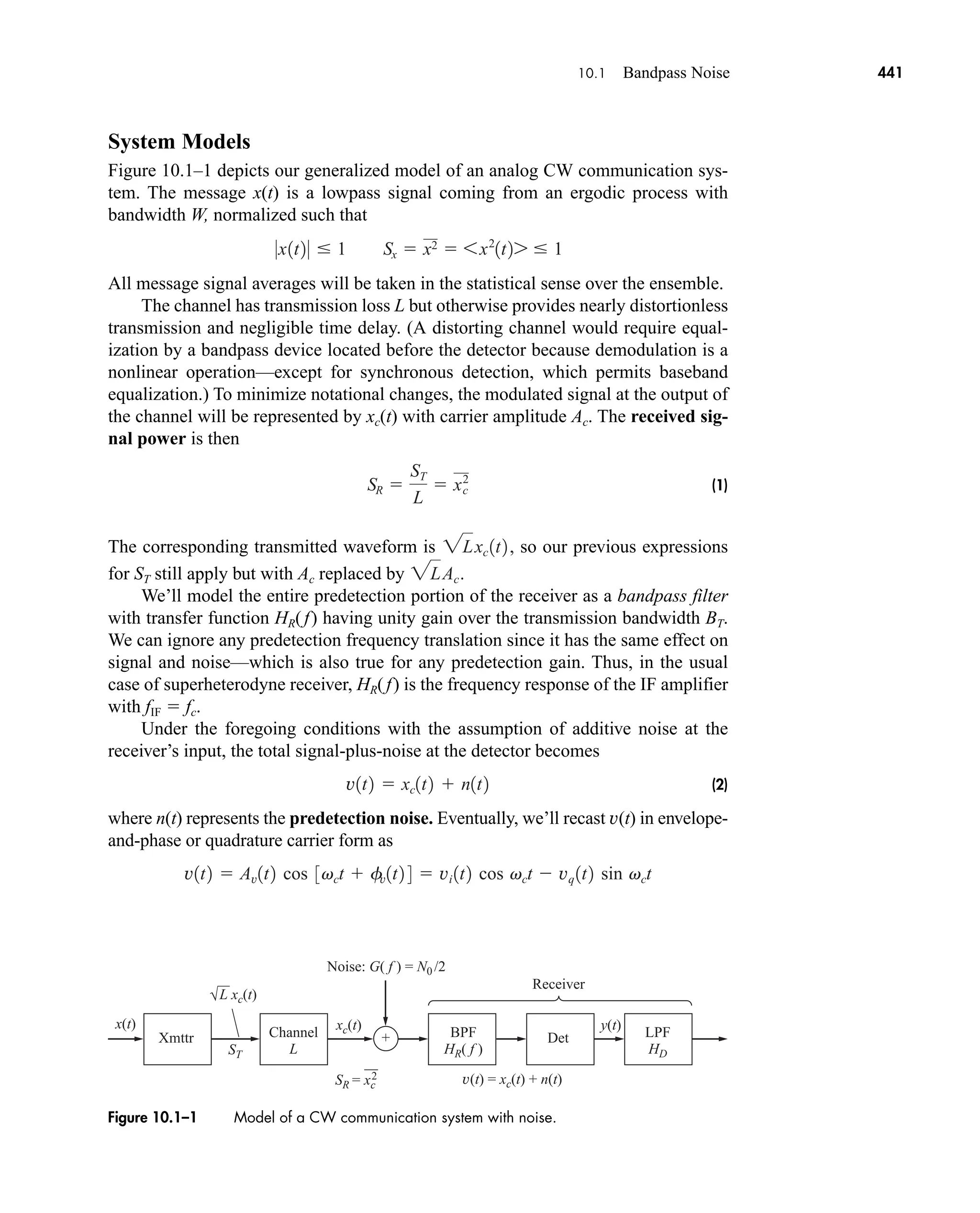
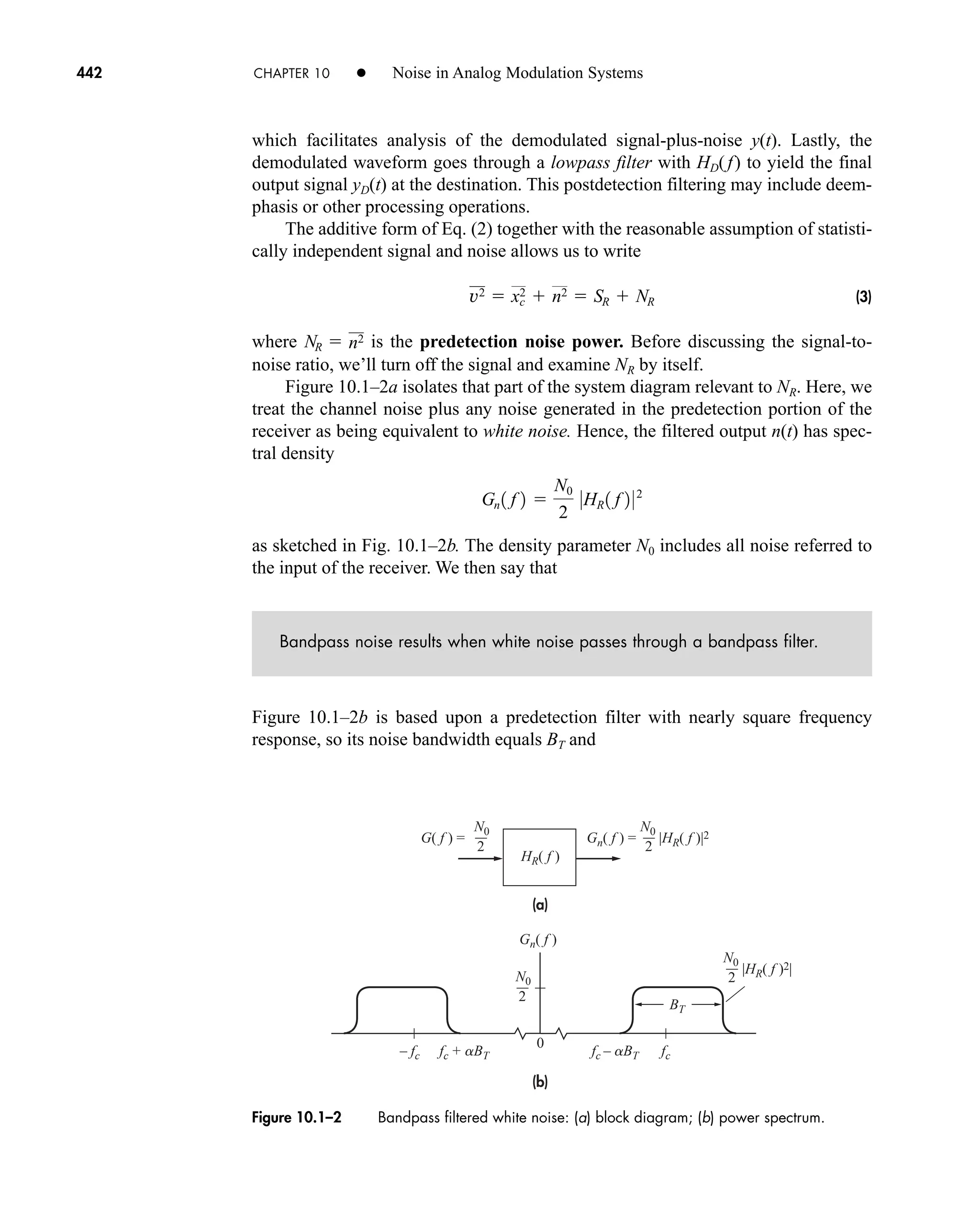
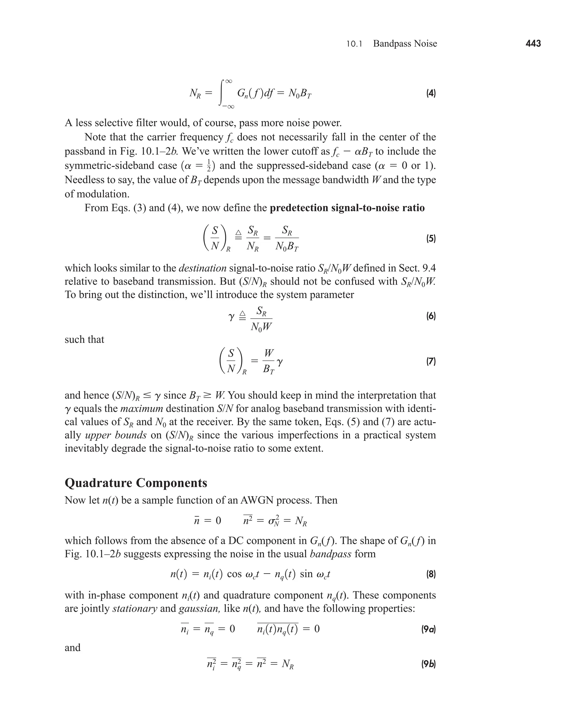
![(a)
(b)
(c)
Gn( f – fc) [1 – u( f + fc)]
– (1 – a)BT (1 – a)BT
– aBT
– BT /2
– BT BT
BT /2
aBT
Gn( f + fc)u( f + fc)
f
f
f
0
0
0
N0 /2
N0 /2
N0
N0
N0 /2
Figure 10.1–3 Lowpass power spectra of the quadrature components of bandpass noise:
(a) general case; (b) symmetric-sideband case; (c) suppressed-sideband case.
444 CHAPTER 10 • Noise in Analog Modulation Systems
Equation (9a) means that the random variables ni(t) and nq(t) are independent at any
instant t, so their joint probability density function is the product of identical gauss-
ian PDF’s.
The power spectral densities of the quadrature components are identical
lowpass functions related to Gn(f) by
(10)
where the term Gn(f fc)u(f fc) simply stands for the positive frequency portion of
Gn(f) translated downward and Gn(f fc)[1 u(f fc)] stands for the negative-
frequency portion translated upward. These terms then overlap and add for f aBT,
as illustrated by Fig. 10.1–3a. Figure 10.1–3b shows the complete overlap in the
symmetric-sideband case (a 1/2), and Fig. 10.1–3c shows the lack of overlap in the
suppressed-sideband case (a 0 or 1). When Gn(f) has local symmetry around fc, as
reflected in Fig. 10.1–3b, the quadrature components are uncorrelated processes.
Sketch Gn(f) and when HR(f) has the VSB shaping shown in Fig. 10.1–4 for
f 0 (this is similar to the actual case in analog television).
Gni
1 f 2
Gni
1 f 2 Gnq
1 f 2 Gn 1 f fc 2u1 f fc 2 Gn 1 f fc 2 31 u1 f fc 2 4
EXERCISE 10.1–1
car80407_ch10_439-478.qxd 12/17/08 5:22 PM Page 444
Confirming Pages](https://image.slidesharecdn.com/communicationsystemsanintro-a-241115060943-61721fa8/75/Communication_Systems__An_Intro_-_A-_Bruce_Carlson_-pdf-466-2048.jpg)
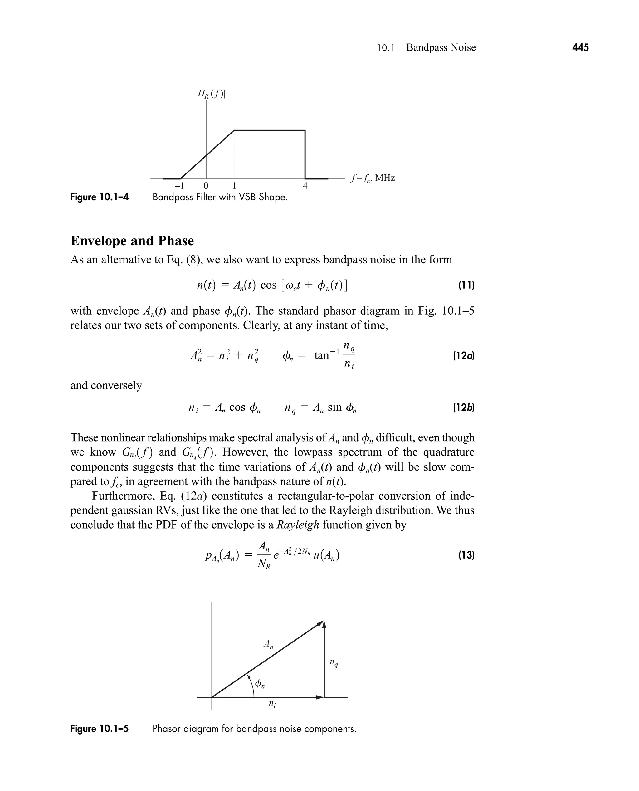
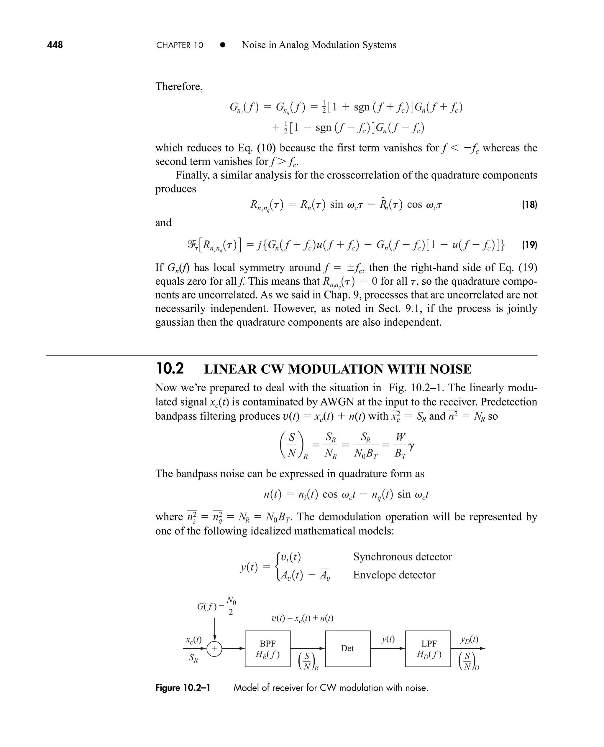
![450 CHAPTER 10 • Noise in Analog Modulation Systems
The preceding analysis is readily adapted to the case of an AM signal
xc(t) Ac[1 x(t)] cos vct, in which we’ve taken m 1 for simplicity. If the syn-
chronous detector includes an ideal DC block, then yD(t) will be as given in Eq. (2),
so and But when we account for the unmodulated carrier power
in we find that SD 2SxSR/(1 Sx) and
(5)
This ratio is bounded by (S/N)D g/2 since Sx 1.
Full-load tone modulation corresponds to Sx 1/2 and (S/N)D g/3, which is
about 5 dB below that of DSB with the same parameters. More typically, however,
Sx 0.1 and AM would be some 10 dB inferior to DSB. AM broadcasting stations
usually combat this effect with special techniques such as volume compression and
peak limiting of the modulating signal to keep the carrier fully modulated most of
the time. These techniques actually distort x(t).
For SSB modulation (or VSB with a small vestige) we have
with BT W and Synchronous
detection rejects the quadrature component of both the signal and noise, leaving
(6)
so Since fc falls at either edge of an ideal predetection filter,
has the shape of Fig. 10.1–3c. Hence,
(7)
and . Therefore,
(8)
which shows that SSB yields the same noise performance as analog baseband or
DSB transmission.
Finally, consider VSB plus carrier. If the vestigial band is small compared to W,
then the predetection and postdetection noise will be essentially the same as SSB.
But the signal will be essentially the same as AM with all the information-bearing
power in one sideband. Hence,
(9)
assuming that BT W and m 1.
To summarize the results in Eqs. (2)–(9), we state the following general proper-
ties of synchronously detected linear modulation with noise:
1. The message and noise are additive at the output if they are additive at the detec-
tor input.
a
S
N
b
D
Sx
1 Sx
a
S
N
b
R
Sx
1 Sx
g VSB C
a
S
N
b
D
a
S
N
b
R
g SSB
ND ni
2 N0W
Gni
1 f 2
N0
2
ß1 f2W 2
Gni
1 f 2
SD Ac
2
˛Sx4 SR .
yD 1t2 1
2 Ac x1t2 ni 1t2
SR Ac
2
˛Sx4.
1Ac22 3x1t2 cos vct x̂1t2 sin vct4
xc1t2
a
S
N
b
D
2Sx
1 Sx
a
S
N
b
R
Sx
1 Sx
g AM
SR Ac
2
11 Sx 22
ND ni
2.
SD Ac
2
Sx
car80407_ch10_439-478.qxd 12/17/08 5:22 PM Page 450
Confirming Pages](https://image.slidesharecdn.com/communicationsystemsanintro-a-241115060943-61721fa8/75/Communication_Systems__An_Intro_-_A-_Bruce_Carlson_-pdf-472-2048.jpg)
![Ac [1 + x]
fv
nq
ni
Av
Figure 10.2–2 Phasor diagram for AM plus noise with (S/N)R W 1.
10.2 Linear CW Modulation with Noise 451
2. If the predetection noise spectrum is reasonably flat over the transmission band,
then the destination noise spectrum is essentially constant over the message
band.
3. Relative to (S/N)D, suppressed-sideband (SSB) modulation has no particular
advantage over double-sideband modulation because the coherence property of
double sideband compensates for the reduced predetection noise power of sin-
gle sideband.
4. Making due allowance for the “wasted” power in unsuppressed-carrier systems,
all types of linear modulation have the same performance as baseband transmis-
sion on the basis of average transmitted power and fixed noise density.
These statements presume nearly ideal systems with fixed average power.
Comparisons based on peak envelope power indicate that SSB yields a postde-
tection S/N about 3 dB better than DSB and 9 dB better than AM, assuming a rea-
sonably smooth modulating signal. But SSB is inferior to DSB if the message has
pronounced discontinuities causing large envelope “horns,” or peaks.
Suppose the predetection filter for a USSB signal actually passes fc W/4 f
fc W. Use Fig. 10.1–3a to sketch the postdetection noise power spectrum. Then
show that (S/N)D will be about 1 dB less than the value predicted by Eq. (8).
Envelope Detection and Threshold Effect
Inasmuch as AM is normally demodulated by an envelope detector, we should exam-
ine how this differs from synchronous detection when noise is present. At the detec-
tor input we have
(10)
where we’re still taking m 1. The phasor construction of Fig. 10.2–2 shows that
the resultant envelope and phase are
(11)
fv 1t2 tan1
nq1t2
Ac 31 x1t2 4 ni 1t2
Av 1t2 25Ac 31 x1t2 4 ni 1t262
3nq1t2 42
v1t2 Ac 31 x1t2 4 cos vct 3ni 1t2 cos vct nq 1t2 sin vct4
EXERCISE 10.2–1
car80407_ch10_439-478.qxd 12/17/08 5:22 PM Page 451
Confirming Pages](https://image.slidesharecdn.com/communicationsystemsanintro-a-241115060943-61721fa8/75/Communication_Systems__An_Intro_-_A-_Bruce_Carlson_-pdf-473-2048.jpg)
![452 CHAPTER 10 • Noise in Analog Modulation Systems
Clearly, further understanding calls for some simplifications, so let’s assume that the
signal is either very large or very small compared to the noise.
Taking the signal to dominate, say then Ac[1 x(t)] will be large
compared to ni(t) and nq(t), at least most of the time. The envelope can then be
approximated by
(12)
which shows the envelope modulation due to noise, similar to interference modula-
tion. An ideal envelope detector reproduces the envelope minus its DC component, so
which is identical to that of a synchronous detector. The postdetection S/N is then as
previously given in Eq. (5). Likewise, Eq. (9) will hold for envelope detection of
VSB C.
However, bear in mind that these results hold only when Since
is proportional to SR/N0BT, an equivalent requirement is (S/N)R W 1. (There is no
such condition with synchronous detection.) Thus, providing that the predetection
signal-to-noise ratio is large, envelope demodulation in the presence of noise has the
same performance quality as synchronous demodulation.
At the other extreme, with (S/N)R V 1, the situation is quite different. For if
the noise dominates in a fashion similar to strong interference, and we can
think of xc(t) as modulating n(t) rather than the reverse. To expedite the analysis of this
case, n(t) is represented in envelope-and-phase form n(t) An(t) cos [vct fn(t)],
leading to the phasor diagram of Fig. 10.2–3. In this figure the noise phasor is the ref-
erence because we are taking n(t) to be dominant. The envelope is then approximated
by the horizontal component, so
(13)
from which
(14)
where
The principal output component is obviously the noise envelope An(t), as expected.
Furthermore, there is no term in Eq. (14) strictly proportional to the message x(t).
An 2pNR2.
y1t2 An 1t2 Acx1t2 cos f
n 1t2 An
Av1t2 An 1t2 Ac 31 x1t2 4 cos f
n 1t2
Ac
2
V n2,
Ac
2
n2
Ac
2
W n2.
yD 1t2 Av 1t2 Av Ac x1t2 ni 1t2
Av 1t2 Ac 31 x1t2 4 ni 1t2
Ac
2
W n2,
An
Ac [1 + x]
Ac [1 + x] cos fn
– fn
Av
Figure 10.2–3 Phasor diagram for AM plus noise with (S/N)R V 1.
car80407_ch10_439-478.qxd 1/13/09 4:19 PM Page 452
Rev.Confirming Pages](https://image.slidesharecdn.com/communicationsystemsanintro-a-241115060943-61721fa8/75/Communication_Systems__An_Intro_-_A-_Bruce_Carlson_-pdf-474-2048.jpg)
![454 CHAPTER 10 • Noise in Analog Modulation Systems
When noise dominates, however, the switching is controlled by the noise peaks and
synchronism is lost. The latter effect never occurs in true synchronous detectors,
where the locally generated carrier can always be much greater than the noise.
Use Eq. (14), Sect. 10.1, to derive the threshold level in Eq. (15a). Specifically, show
that if Sx 1, then P(Ac An) 0.99 requires (S/N)R 4 ln 10 10.
10.3 ANGLE CW MODULATION WITH NOISE
This section deals with noise in analog PM and FM systems. The demodulation
operation will be represented by
As we saw in Chap. 5, the inherent nonlinear nature of angle modulation leads to
analytic difficulties—all the more so when noise must be considered. We’ll therefore
begin with the large signal condition (S/N)R W 1 to determine the postdetection
noise characteristics and signal-to-noise ratios for PM and FM. Our efforts here pay
off in results that quantify the valuable wideband noise reduction property, a prop-
erty further enhanced by postdetection FM deemphasis filtering.
Importantly, wideband noise reduction involves a threshold effect that, unlike the
AM case, may pose a significant performance limitation. We’ll qualitatively discuss
operation near threshold, and take a brief look at the FM feedback receiver as one
technique for threshold extension.
Postdetection Noise
The predetection portion of an angle modulation receiver has the structure previ-
ously diagrammed in Fig. 10.2–1. The received signal is
where f(t) f x(t) for a PM wave or for an FM wave. In either
case, the carrier amplitude remains constant so
(1)
and (S/N)R is often called the carrier-to-noise ratio (CNR). The predetection BPF is
assumed to have a nearly ideal response with bandwidth BT centered at fc.
Figure 10.3–1 portrays our model for the remaining portion of the receiver, with
the detector input v(t) xc(t) n(t) Av(t) cos [vct fv(t)]. The limiter suppresses
SR 1
2 Ac
2
a
S
N
b
R
Ac
2
2N0BT
f
#
1t2 2pf¢x1t2
xc1t2 Ac cos 3vct f1t2 4
y1t2 c
f
v1t2 Phase detector
1
2p f
#
v1t2 Frequency detector
EXERCISE 10.2–2
car80407_ch10_439-478.qxd 6/1/09 7:54 AM Page 454
Rev. Confirming Pages](https://image.slidesharecdn.com/communicationsystemsanintro-a-241115060943-61721fa8/75/Communication_Systems__An_Intro_-_A-_Bruce_Carlson_-pdf-476-2048.jpg)
![fv – f fn – f
Ac
An
Av
Figure 10.3–2 Phasor diagram of angle modulation plus noise.
N0BT y(t) =
v(t) = xc(t) + n(t) = Av(t) cos [vct + fv(t)]
fv(t) PM
fv(t) FM
BPF
HD( f )
Discriminator
Limiter
= ––––––
1
2p
Ac/2
2
R
( )
N
S
yD(t)
.
Figure 10.3–1 Model for detection of angle modulation plus noise.
10.3 Angle CW Modulation with Noise 455
any amplitude variation represented by Av(t). To find the signal and noise contained
in fv(t), we express n(t) in envelope-and-phase form and write
(2)
The phasor construction of Fig. 10.3–2 then shows that
(3)
The first term of fv(t) is the signal phase by itself, but the contaminating second term
involves both noise and signal. Clearly, this expression is very unclear and we can’t
go much further without some simplifications.
A logical simplification comes from the large-signal condition (S/N)R W 1, so
Ac W An(t) most of the time and we can use the small-argument approximation for
the inverse tangent function. A less obvious simplification ignores f(t) in Eq. (3),
replacing fn(t) f(t) with fn(t) alone. We justify this step for purposes of noise
analysis by recalling that fn has a uniform distribution over 2p radians; hence, in the
sense of ensemble averages, fn f differs from fn only by a shift of the mean
value. With these two simplifications Eq. (3) becomes
(4)
where
(5)
in which we’ve substituted nq An sin fn and SR Ac
2
2.
c1t2
^ An sin f
n1t2
Ac
1
22SR
nq 1t2
fv1t2 f1t2 c1t2
fv1t2 f1t2 tan1
An 1t2 sin 3fn 1t2 f1t2 4
Ac An 1t2 cos 3fn 1t2 f1t2 4
v1t2 Ac cos 3vct f1t2 4 An 1t2 cos 3vct f
n 1t2 4
car80407_ch10_439-478.qxd 6/1/09 7:54 AM Page 455
Rev. Confirming Pages](https://image.slidesharecdn.com/communicationsystemsanintro-a-241115060943-61721fa8/75/Communication_Systems__An_Intro_-_A-_Bruce_Carlson_-pdf-477-2048.jpg)
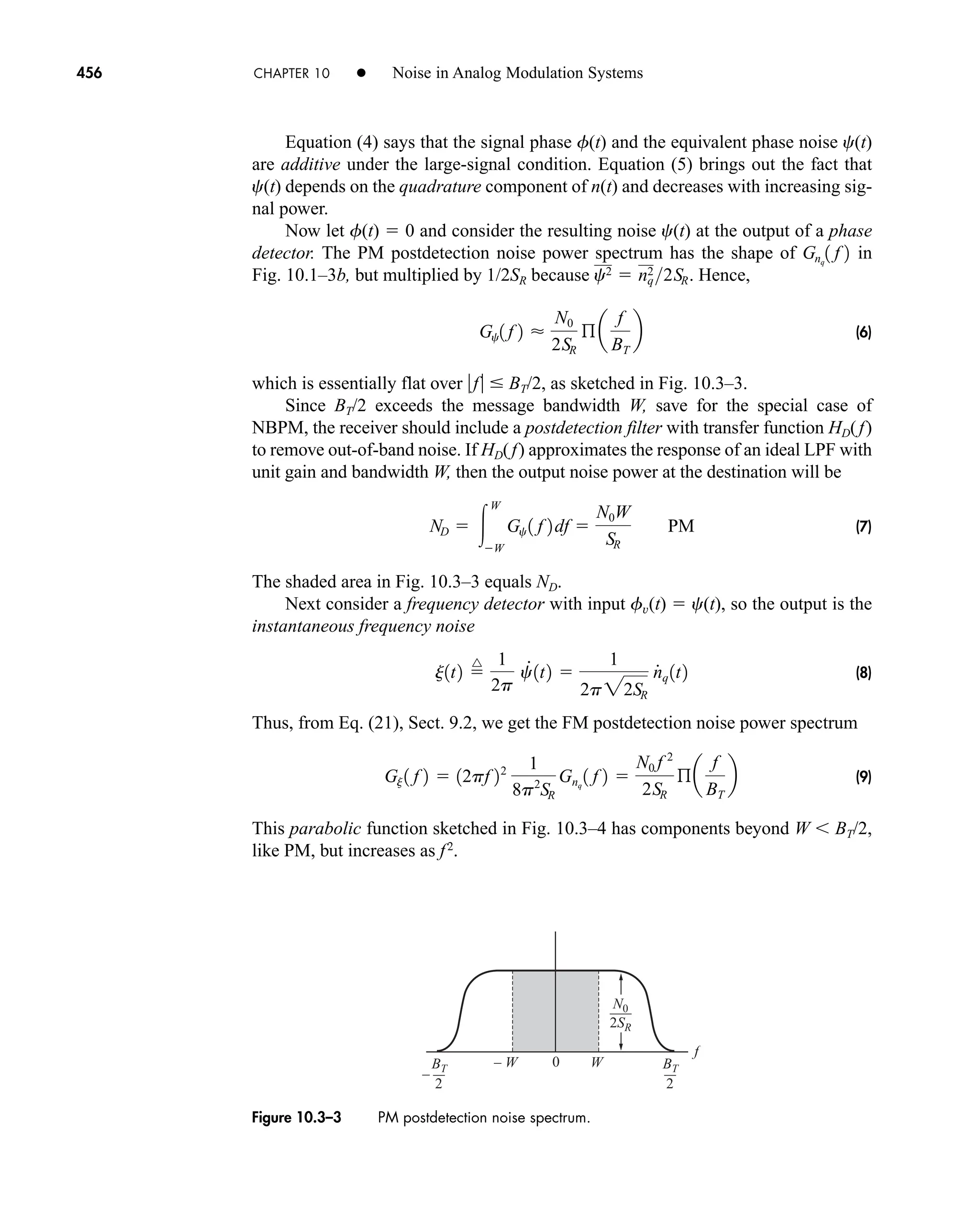
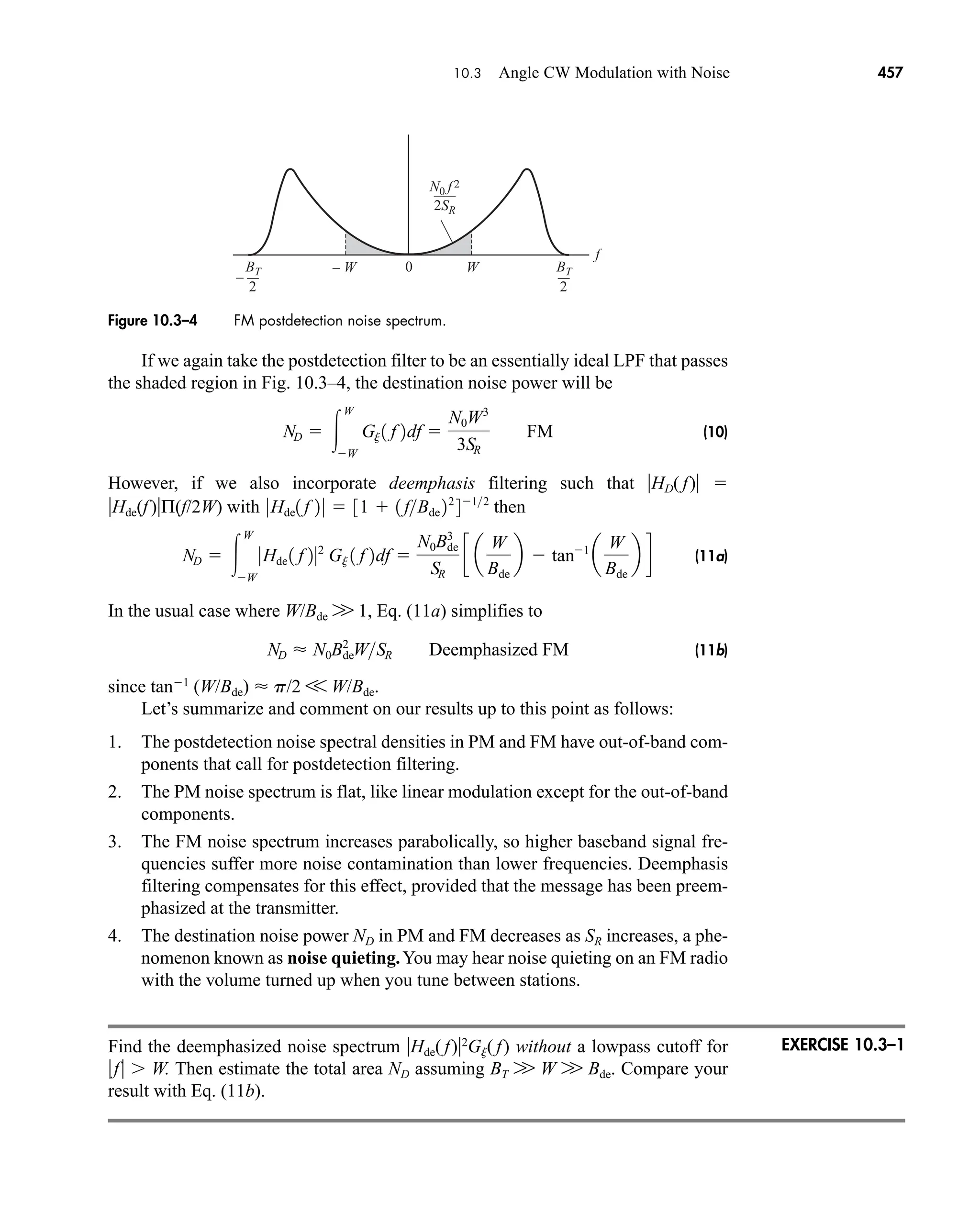
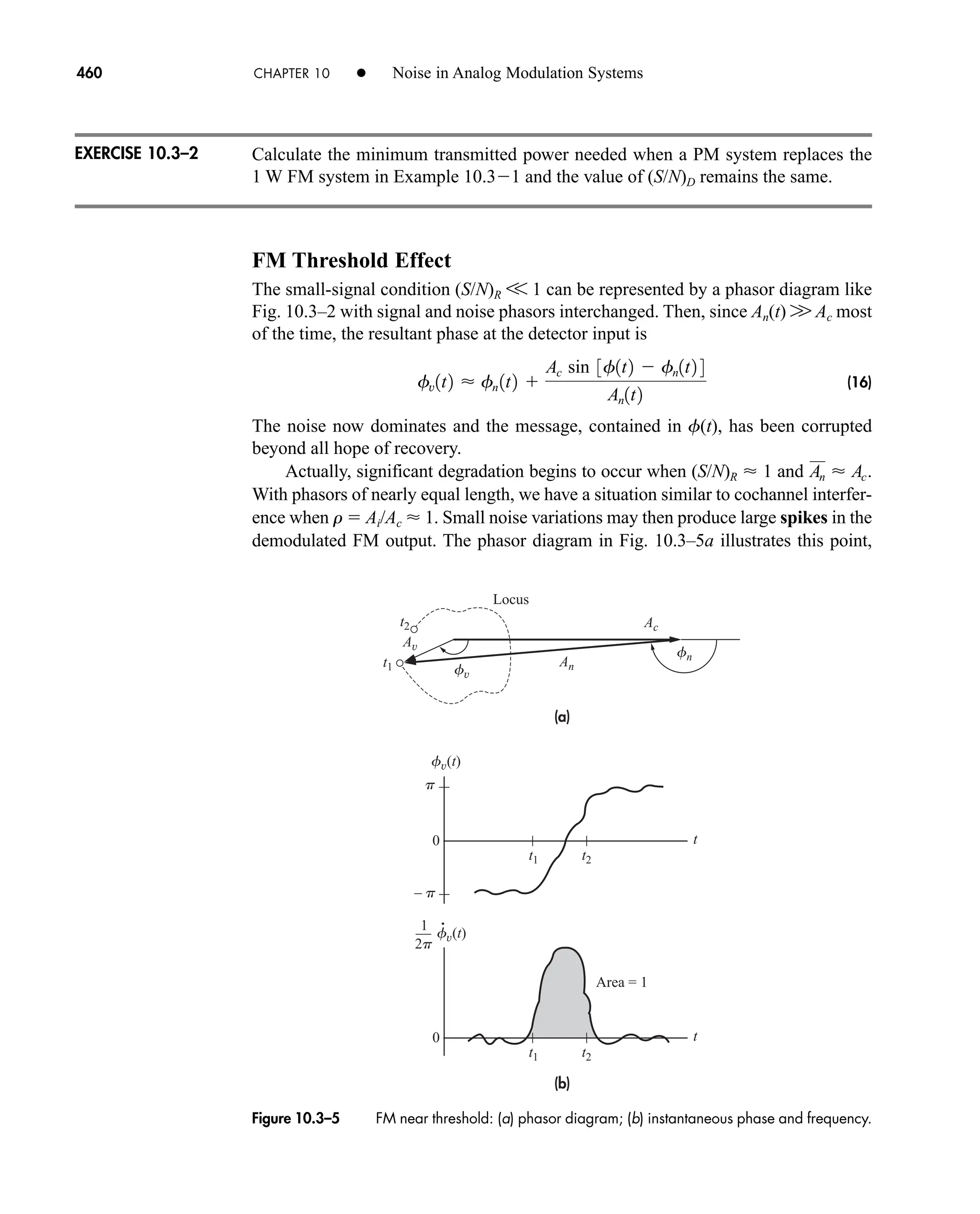
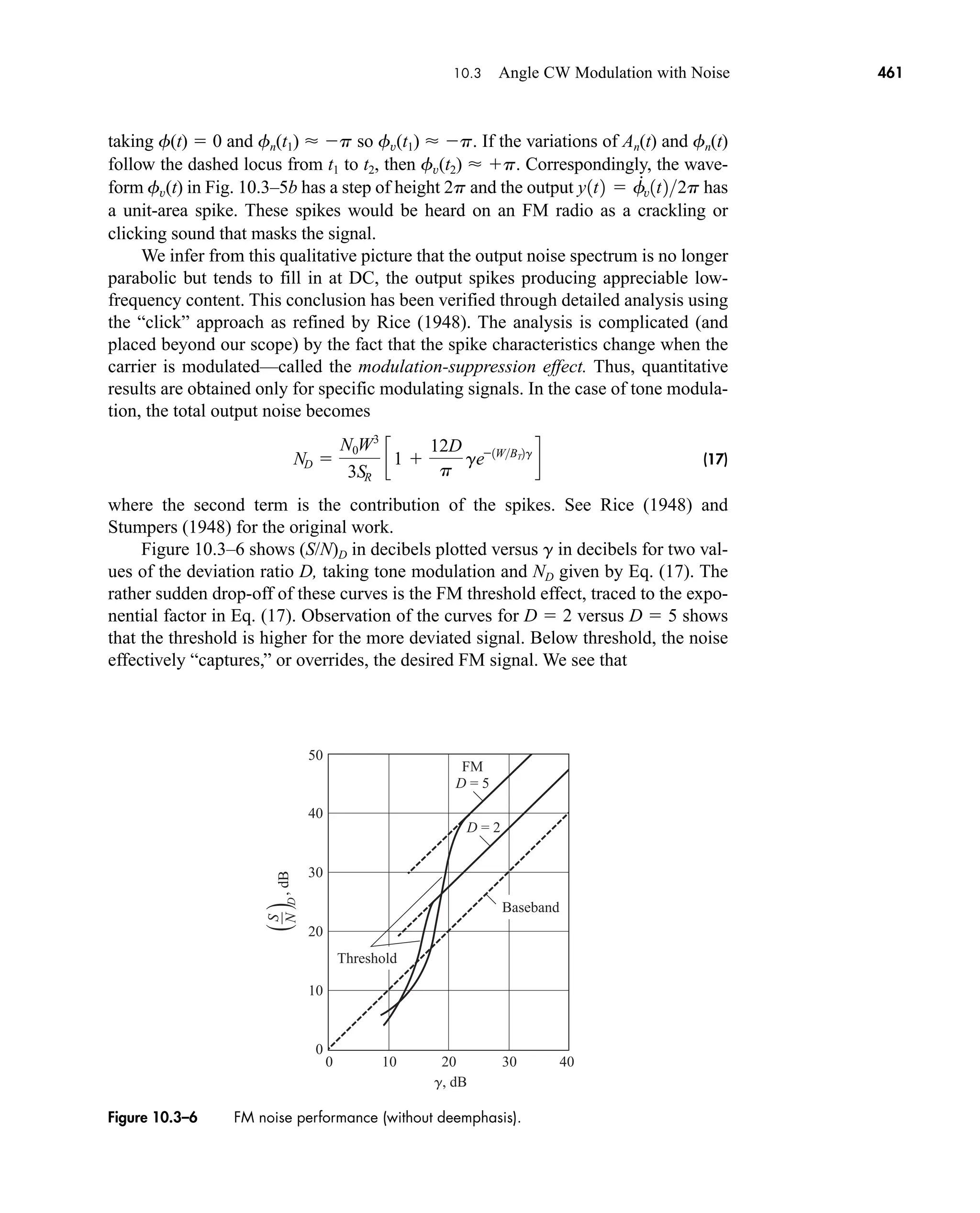
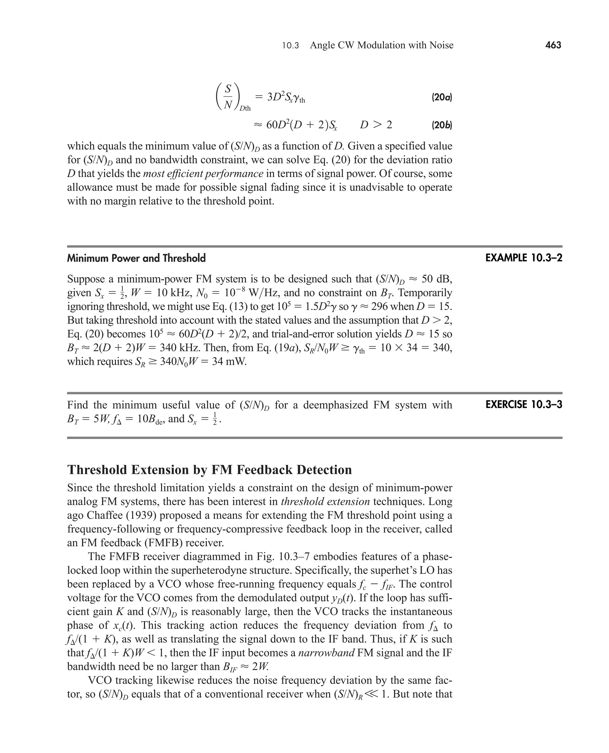
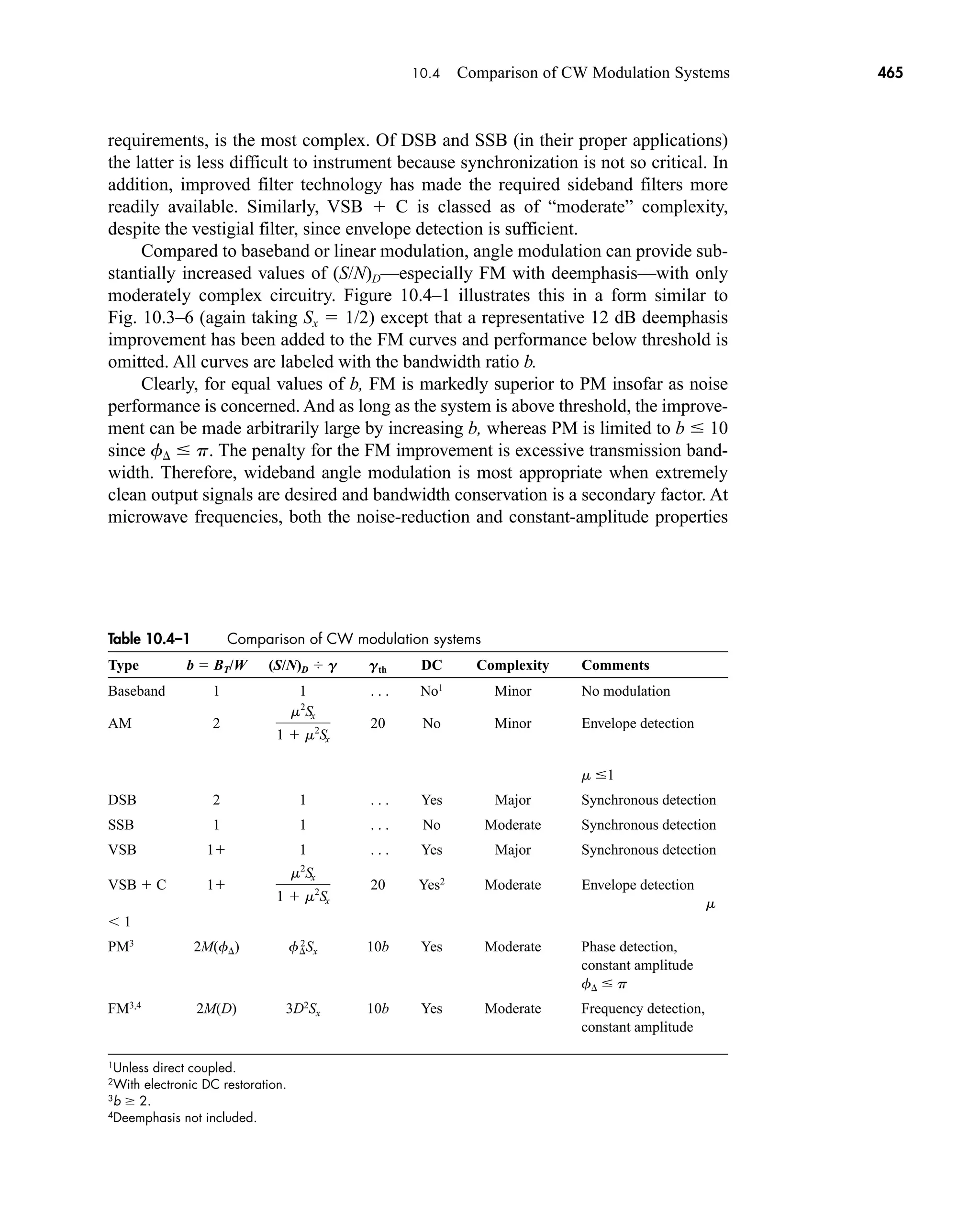
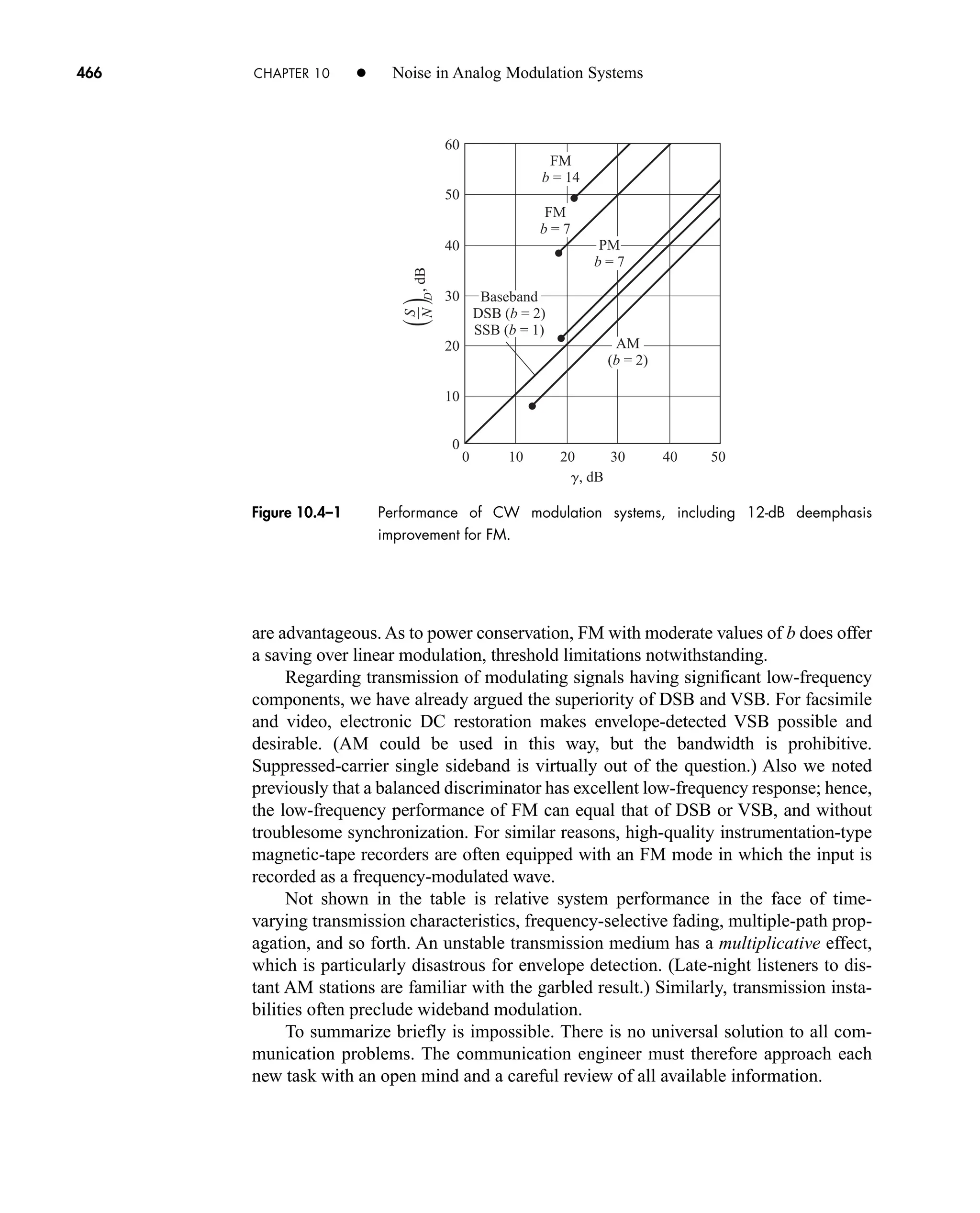
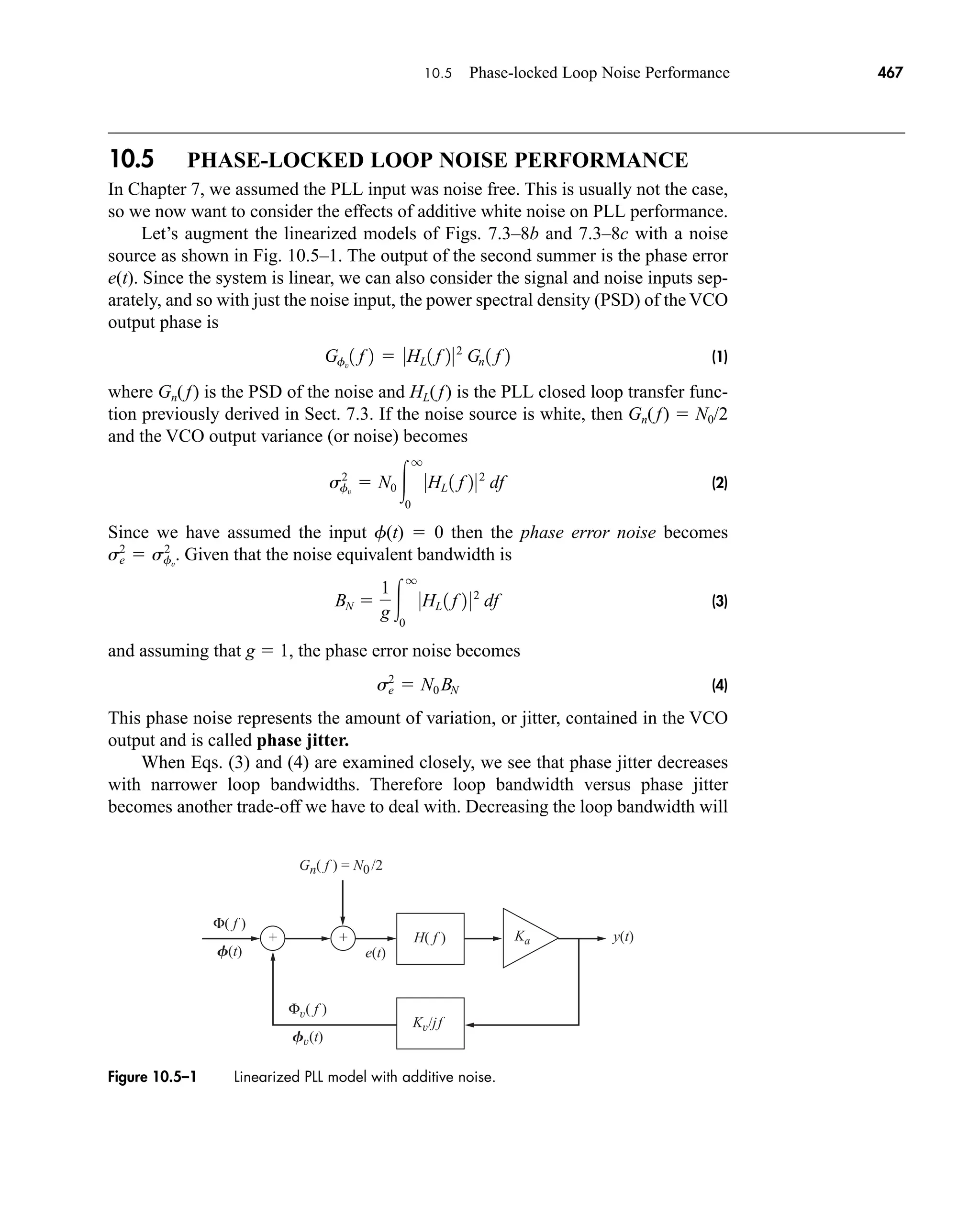
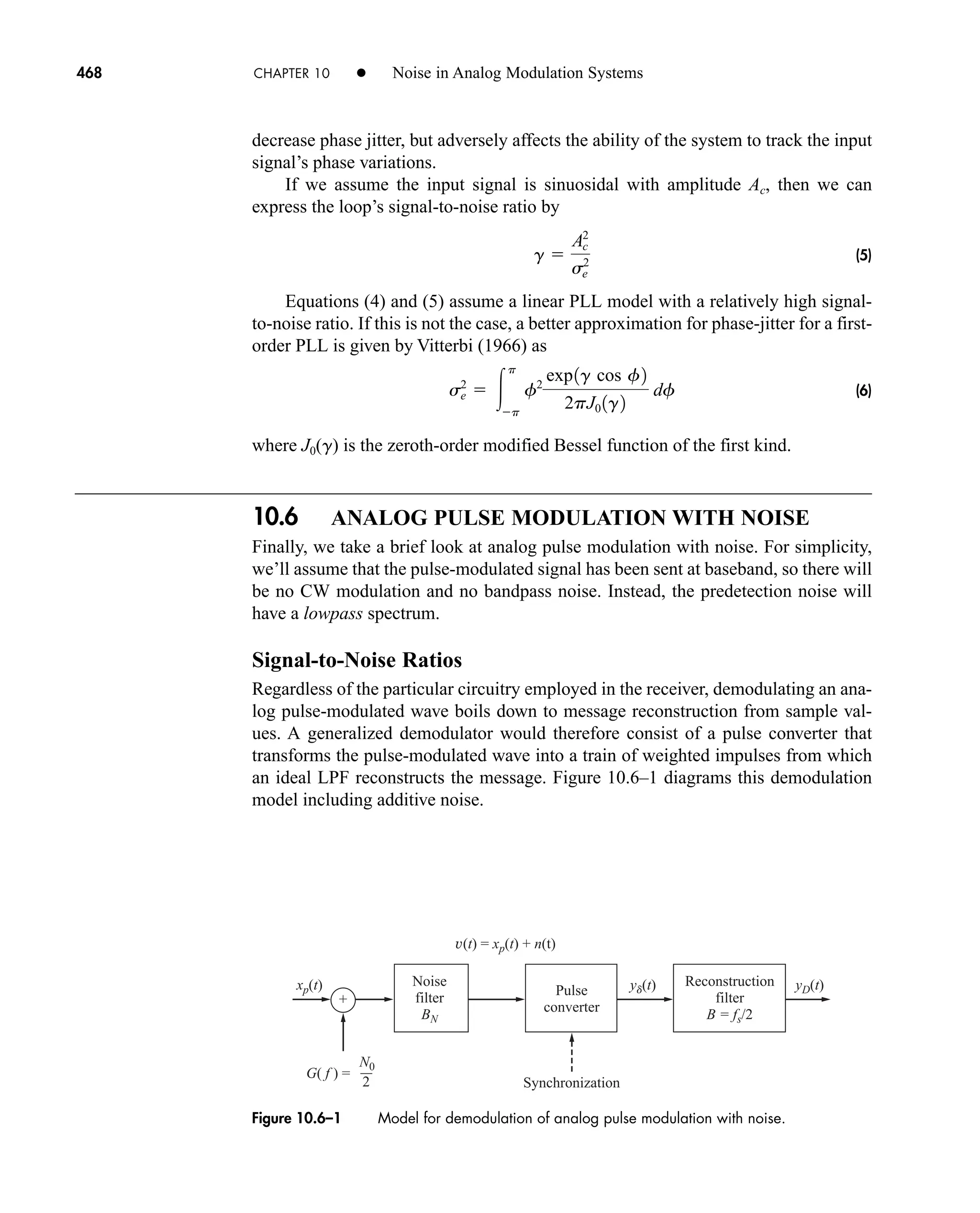
![10.6 Analog Pulse Modulation with Noise 469
A noise-limiting filter at the input passes the received pulsed signal xp(t) plus
lowpass noise n(t), so v(t) xp(t) n(t). The converter measures the amplitude,
duration, or position of each pulse in v(t) and generates
(1)
where mp is the modulation constant relating x(kTs) to xp(t) and k is the measurement
error induced by the noise. We’ll assume for convenience that the reconstruction fil-
ter has bandwidth B fs/2, gain K Ts 1/2B, and zero time delay. Hence, the
impulse-train input yd(t) produces the final output
(2a)
with
(2b)
which represents the noise at the destination.
Since the errors k are proportional to sample values of the lowpass noise n(t)
spaced by Ts, and since the noise-limiting filter has BN 1/Ts, the values of k will be
essentially uncorrelated and will have zero mean. We can therefore write the destina-
tion noise power as and the signal power is
Hence,
(3)
which expresses the destination signal-to-noise ratio in terms of the error variance s2
caused by reconstruction from noisy samples. Our next task is to determine and
s2
for specific types of analog pulse modulation.
A PAM signal contains the message samples in the modulated pulse amplitude
A0[1 mx(kTs)], so the modulation constant is mp A0m A0. From Sect. 9.5,
the amplitude error variance is Thus, under the best conditions
of maximum modulation (m 1) and minimum noise bandwidth (BN 1/2t),
we have
where t is the pulse duration.
When m 1 and x(t) has no DC component, the average energy per modulated
pulse is Multiplying this average energy by the
pulse rate fs gives the received signal power We thus obtain our
final result in the form
SR fs˛A0
2
11 Sx 2t.
A0
2
31 x1kTs 2 42
˛
t A0
2
11 Sx 2t.
a
S
N
b
D
2A0
2
t
N0
Sx
s2
sA
2
N0BN .
mp
2
a
S
N
b
D
SD
ND
mp
2
s2 Sx
SD m2
px2 mp
2
Sx.
ND nD
2 Pk
2 s2
nD 1t2 a
k
Pk sinc 1 fs t k2
yD 1t2 a
k
3mp x1kTs 2 Pk 4 sinc 1 fst k2 mp x1t2 nD 1t2
yd1t2 a
k
3mpx1kTs 2 Pk 4d1t kTs 2
car80407_ch10_439-478.qxd 12/17/08 5:22 PM Page 469
Confirming Pages](https://image.slidesharecdn.com/communicationsystemsanintro-a-241115060943-61721fa8/75/Communication_Systems__An_Intro_-_A-_Bruce_Carlson_-pdf-491-2048.jpg)
![10.7 Questions and Problems 473
property (a) Let and
show that we can write
(b) Use this result to show that
10.1–5 A tuned circuit with Q fc/BT W 1 approximates the local-symmetry
property in Prob. 10.1–4, and has HR( f) 1/[1 j2(f fc)/BT] for f 0.
(a) Find Gp(f). (b) Evaluate by calculating
10.1–6 Let y(t) 2n(t) cos (vct u), where n(t) is bandpass noise centered at fc.
Show that y(t) consists of a lowpass component and a bandpass compo-
nent. Find the mean value and variance of each component in terms of
the properties of n(t).
10.1–7* Bandpass gaussian noise with sN 2 is applied to an ideal envelope detec-
tor, including a DC block. Find the PDF of the output y(t) and calculate sY.
10.1–8 Bandpass gaussian noise with variance is applied to an ideal square-
law device, producing Find and the PDF of y(t).
10.1–9 Let Assuming that v(t) is Fourier trans-
formable, show that Vp( f) [vp(t)] V(f fc)u(f fc). Then sketch
Vp( f), taking V( f) as in Fig. P10.1–1 with fc f1 b.
10.1–10* Let HR( f) in Fig. 10.1–2 be an ideal BPF with unit gain and let so
fc is the center frequency. Find Rn(t) and by taking the inverse
transform of Gn( f) and (j sgn f)Gn( f). Then obtain from Eq.
(17) and confirm that it equals the inverse transform of
10.1–11 Do Prob. 10.1–10 with a 0, so fc is the lower cutoff frequency.
10.1–12 Suppose Gn(f) has local symmetry around fc, as detailed in Prob. 10.1–4.
Write the inverse transforms of and Gn( f ) to show that
Then show from Eq. (17) that
10.1–13 Derive Eq. (17) starting from E[nq(t)nq(t t)].
10.1–14 Derive Eq. (18) starting from E[nq(t)nq(t t)].
10.1–15 Let Gn(f) have local symmetry around fc. Prove that for
all t using: (a) the correlation relations in Prob. 10.1–12; (b) the spectral
relations in Prob. 10.1–4.
10.1–16* Let HR(f) in Fig. 10.1–2 be an ideal BPF with unit gain and let a 0, so
fc is the lower cutoff frequency. Use Eq. (19) to find
10.1–17 Do Prob. 10.1–16 with a 1/4, so the lower cutoff frequency is
fc BT/4.
10.1–18 What is the expression for the output of a synchronous detector if the
input is bandpass gaussian noise?
Rninq
1t2.
Rninq
1t2 0
R̂n1t2 Rni
1t2 sin vct.
Rni
1t2 cos vct.
Rn 1t2
Gni
1 f 2
Gni
1 f 2.
Rni
1t2
R̂n1t2
a 1
2
v/p1t2 1
2 3v1t2 jv̂1t2 4ejvct
.
y, y2
,
y1t2 An
2
1t2.
sN
2
ni
2
.
n2
Gni
1 f 2 2G/p1 f 2.
Gn1 f 2 G/p 1 f fc 2 G/p1 f fc 2 e
G/p 1 f fc 2 f 7 0
G/p 1 f fc 2 f 6 0
G/p1 f 2
^
1N022 0H/p1 f 202
0H/p1f 20 0H/p1 f 20.
car80407_ch10_439-478.qxd 12/17/08 5:22 PM Page 473
Confirming Pages](https://image.slidesharecdn.com/communicationsystemsanintro-a-241115060943-61721fa8/75/Communication_Systems__An_Intro_-_A-_Bruce_Carlson_-pdf-495-2048.jpg)
![474 CHAPTER 10 • Noise in Analog Modulation Systems
10.2–1* A DSB signal plus noise is demodulated by synchronous detection. Find
(S/N)D in dB given that SR 20 nW, W 5 MHz, and N 100.
10.2–2 An AM signal plus noise is demodulated by synchronous detection. Find
(S/N)D in dB given that Sx 0.4, SR 20 nW, W 5 MHz, m 1, and
N 100.
10.2–3 A DSB signal plus noise is demodulated by a product detector with
phase error f . Take the local oscillator signal to be 2 cos (vct f ) and
show that (S/N)D g cos2
f .
10.2–4 Rewrite Eqs. (4b) and (5) in terms of gp Sp/N0W, where Sp is the peak
envelope power of the DSB or AM signal.
10.2–5* Let xc(t) have quadrature multiplexing, where x1(t) and x2(t) are inde-
pendent signals and Assume an ideal receiver with AWGN and
two synchronous detectors. Find the output signal plus noise for each
channel, and express (S/N)D in terms of g.
10.2–6 Explain why an SSB receiver should have a nearly rectangular BPF with
bandwidth BT W, whereas predetection filtering is not critical for DSB.
10.2–7 Modify Eq. (8) for LSSB when HR(f )2
has the shape in Fig. P10.1–1
with f2 fc and 2b W.
10.2–8 Some receivers have additive “one-over-f”(1/f) noise with power spectral
density G( f ) N0 fc/2f for f 0. Obtain the resulting expressions for
(S/N)D in terms of g and W/fc for USSB and DSB modulation. Compare
your results when W/fc 1/5 and 1/50.
10.2–9‡
When a demodulated signal includes multiplicative noise or related
effects, the postdetection S/N cannot be defined unambiguously. An
alternative performance measure is then the normalized mean-square
error where K is chosen such that
KyD(t) x(t) in absence of multiplicative effects. Find yD(t) and show
that when a USSB signal with AWGN is
demodulated by a product detector whose local-oscillator signal is 2 cos
[vct f(t)], where f(t) is a slowly drifting random phase. Hint:
and since is an odd function.
10.2–10 Explain why an AM receiver should have a nearly rectangular BPF with
bandwidth BT 2W for envelope detection, whereas predetection filter-
ing is not critical for synchronous detection.
10.2–11* An AM system with envelope detection is operating at the threshold
point. Find the power gain in dB needed at the transmitter to get up to
(S/N)D 40 dB with full-load tone modulation.
10.2–12 An AM system with envelope detection has (S/N)D 30 dB under full-
load tone-modulation conditions with W 8 kHz. If all bandwidths are
R̂x 1t2
x x̂ R̂x 102 0
x̂2
x2
P2
231 cos f 4 1g
P2
^
E53x1t2 KyD 1t2 42
6Sx
x2
1
x2
2
.
car80407_ch10_439-478.qxd 12/17/08 5:22 PM Page 474
Confirming Pages](https://image.slidesharecdn.com/communicationsystemsanintro-a-241115060943-61721fa8/75/Communication_Systems__An_Intro_-_A-_Bruce_Carlson_-pdf-496-2048.jpg)
![476 CHAPTER 10 • Noise in Analog Modulation Systems
10.3–10* Obtain an expression like Eq. (20) for PM, and determine the upper
bound on (S/N)D at threshold.
10.3–11 Consider the FMFB receiver in Fig. 10.3–7. Let v(t) be a noise-free FM
signal with deviation ratio D and take the VCO output to be 2 cos
[(vc vIF)t KfD(t)] where Show that the deviation
ratio of the IF signal is DIF D/(1 K).
10.3–12 Let’s assume you are allowed to broadcast without a license if you stay
below the ambient level of radiation is 75 nW/MHz. Measurements have
determined that in the general listening area, an ordinary DSB transmis-
sion is received with (S/N)R 30 dB, W 3 kHz, and SR 1 mW.
Design an FM system that will enable unlicensed broadcasting for
W 3 kHz messages.
10.3–13 What is the maximum value of N0 for an FM cell phone whereby
ST 3 W, f 12 kHz, W 3 kHz, Sx 0.5, f 850 MHz, and cell to
tower distance is 1.6 kM?
10.4–1* An analog communication system has W 10 kHz, N0
1015
W/Hz, and transmission loss L 100 dB. Calculate ST needed to
get (S/N)D 40 dB when the modulation is (a) SSB; (b) AM with m 1
and m 0.5; (c) PM with f p; (d) FM with D 1, 5, and 10. Omit
deemphasis in the FM case, but check for threshold limitations.
10.4–2 Do Prob. 10.4–1 with and W 20 kHz.
10.4–3 An analog communication system has W 10 kHz, ST 10
W, and N0 1013
W/Hz. Calculate the path length corresponding to
(S/N)D 40 dB for a transmission cable with loss factor a 1 dB/km
when the modulation is (a) SSB; (b) AM with m 1; (c) FM with D 2
and 8.
10.4–4 Do Prob. 10.4–3 for line-of-sight radio transmission at fc 300 MHz
with antenna gains of 26 dB at transmitter and receiver.
10.4–5* A signal with is transmitted via AM with m 1 and (S/N)D
13 dB. If the modulation is changed to FM (without deemphasis) and the
bandwidths are increased accordingly while other parameters remain
fixed, what’s the largest usable deviation ratio and the resulting value of
(S/N)D?
10.4–6‡
A frequency-division multiplexing system has USSB subcarrier modula-
tion and FM carrier modulation without preemphasis. There are K
independent input signals, each having bandwidth W0, and the subcarrier
frequencies are fk (k 1)W0, k 1, 2, . . . K. The baseband signal at
the FM modulator is xb(t) Σ akxk(t), where the ak are constants and
xk(t) is the kth subcarrier signal, each having The discriminator
at the receiver is followed by a bank of BPFs and synchronous detectors.
xk
2
1.
x2 12
x2 12,
x2 1
x2 12,
f
#
D1t2 2pyD1t2.
car80407_ch10_439-478.qxd 12/17/08 5:22 PM Page 476
Confirming Pages](https://image.slidesharecdn.com/communicationsystemsanintro-a-241115060943-61721fa8/75/Communication_Systems__An_Intro_-_A-_Bruce_Carlson_-pdf-498-2048.jpg)


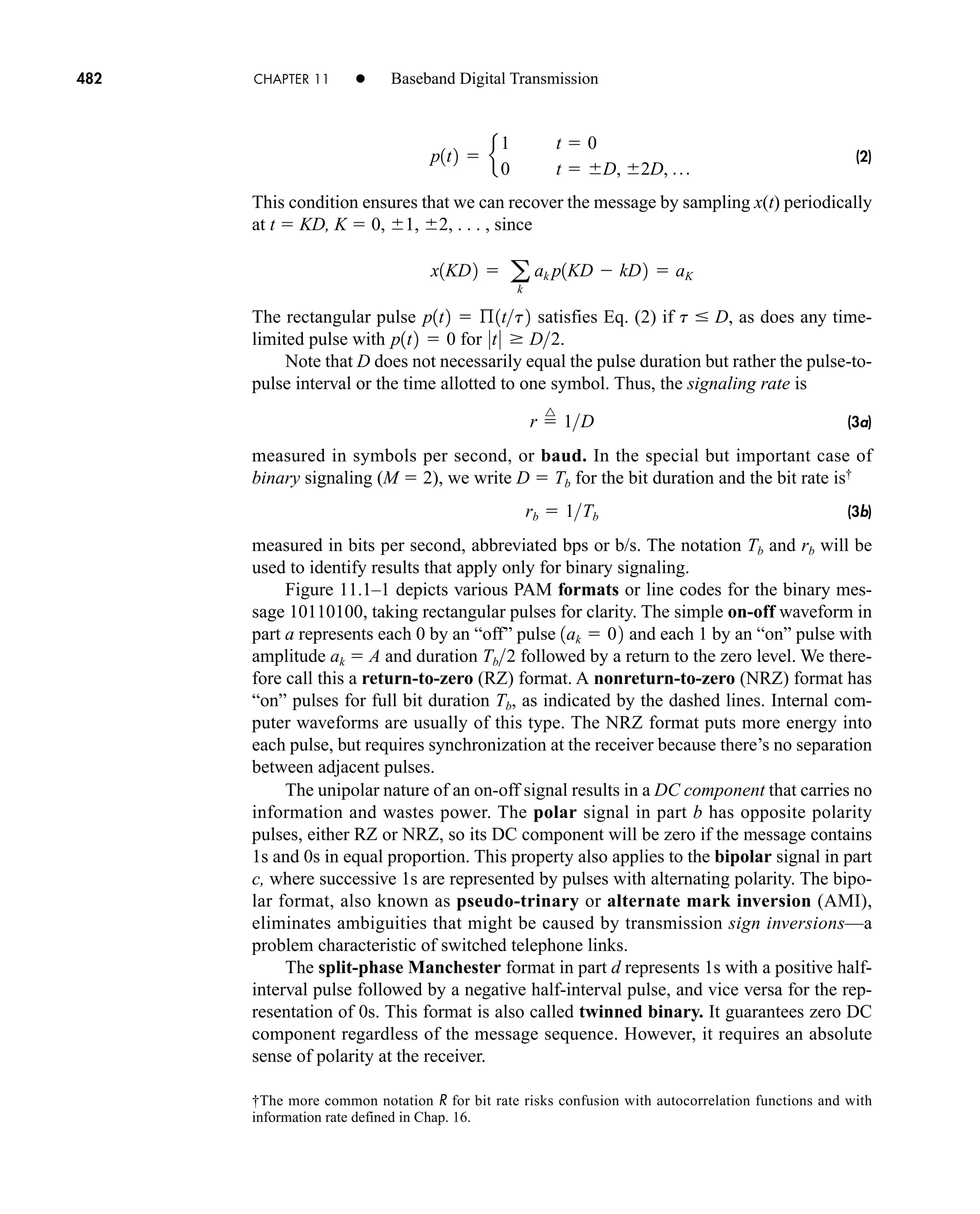
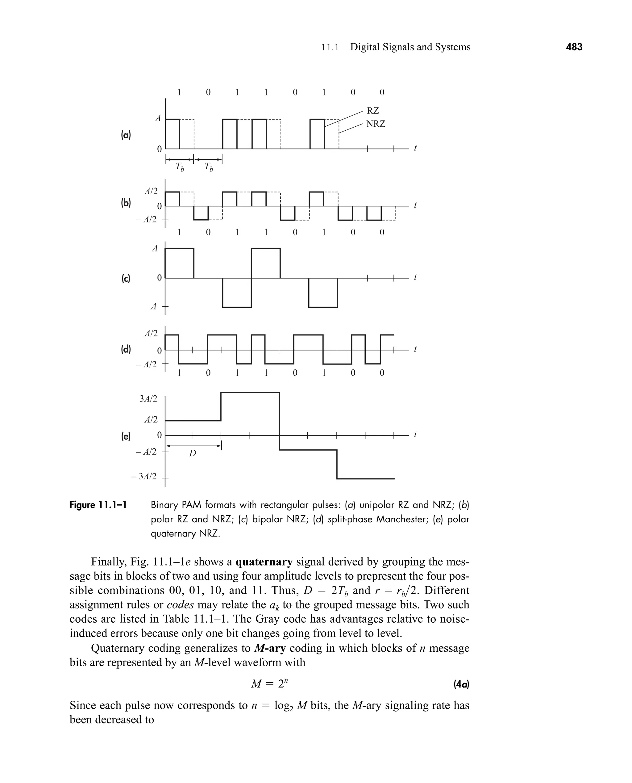
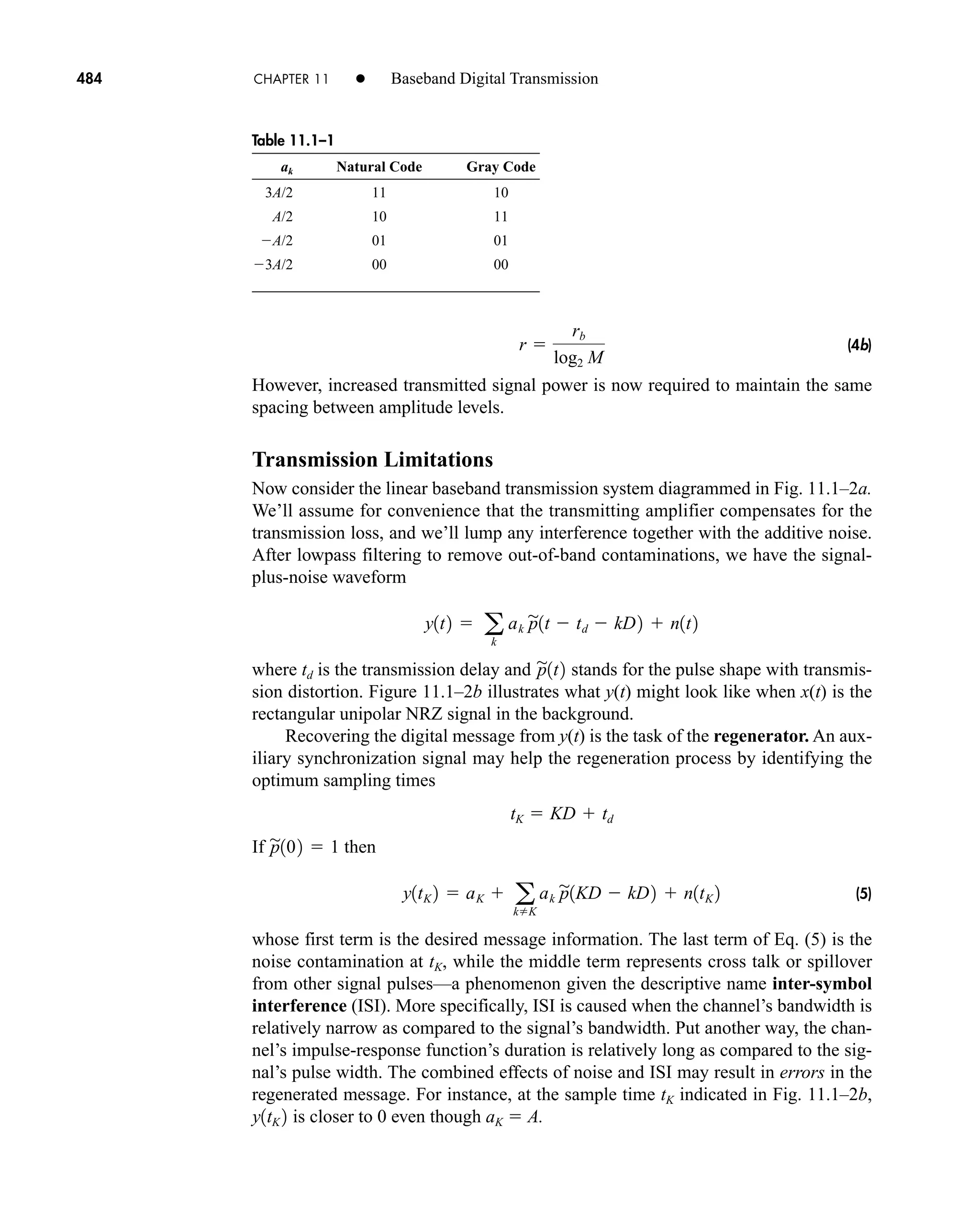
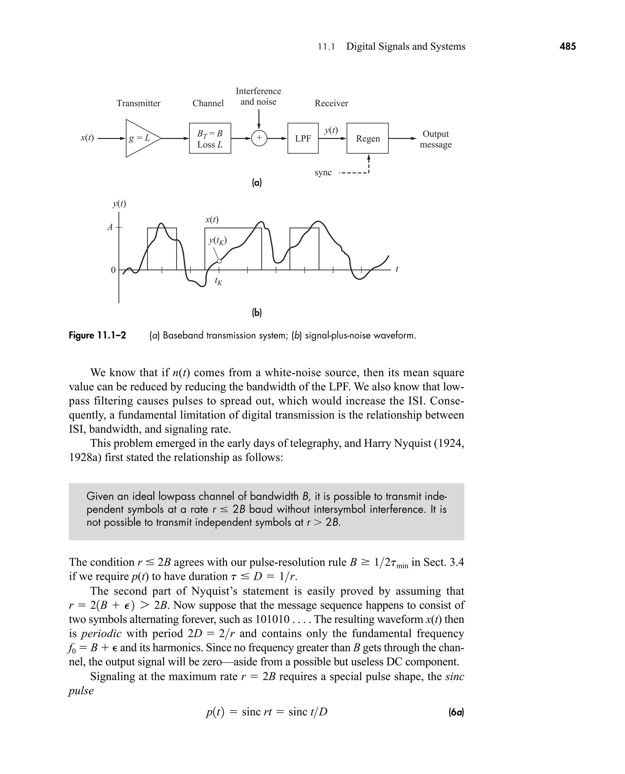
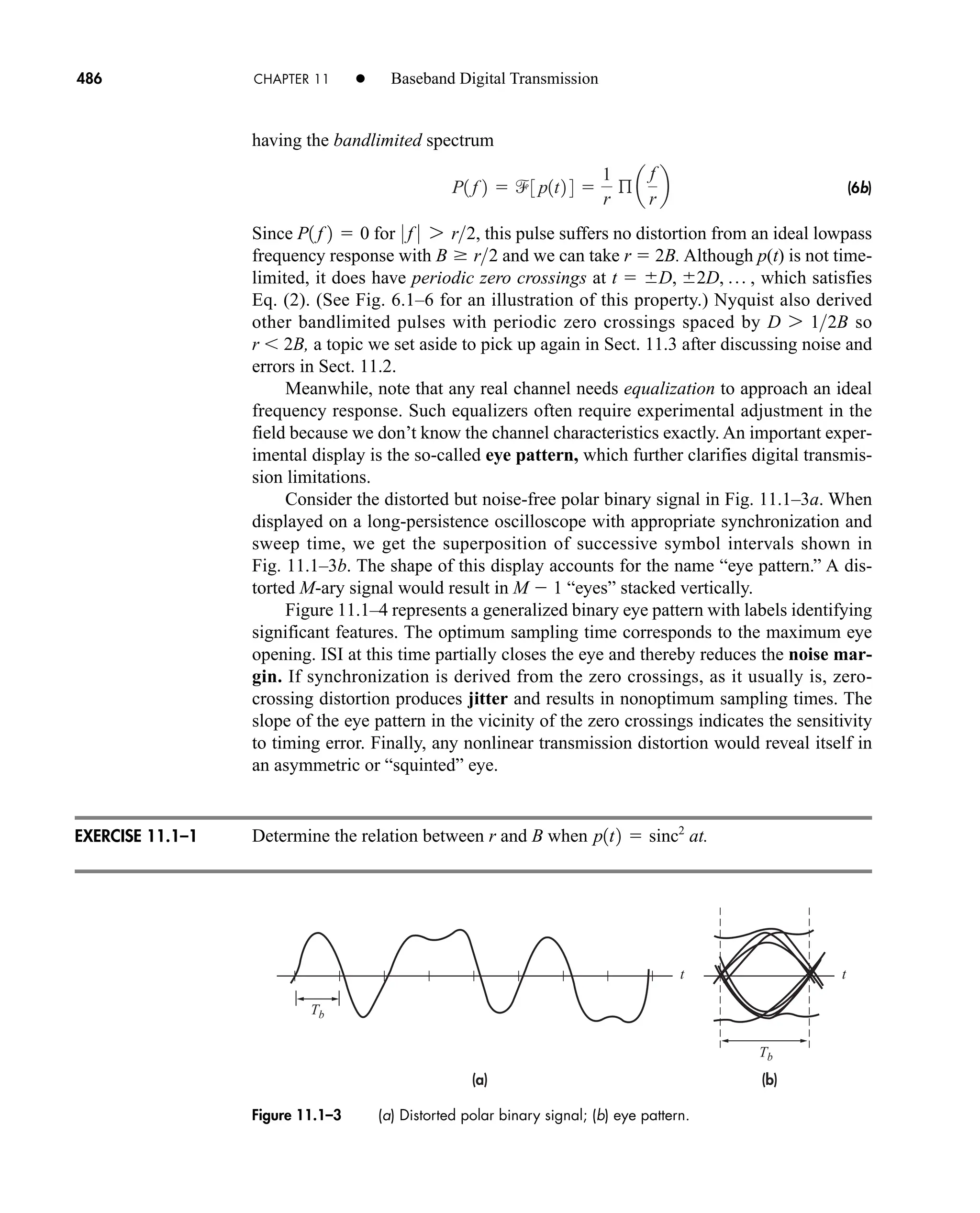
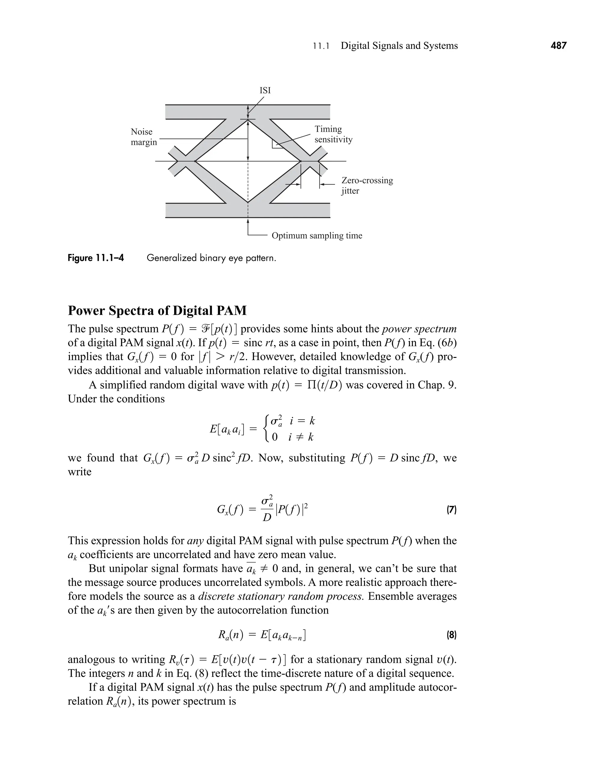
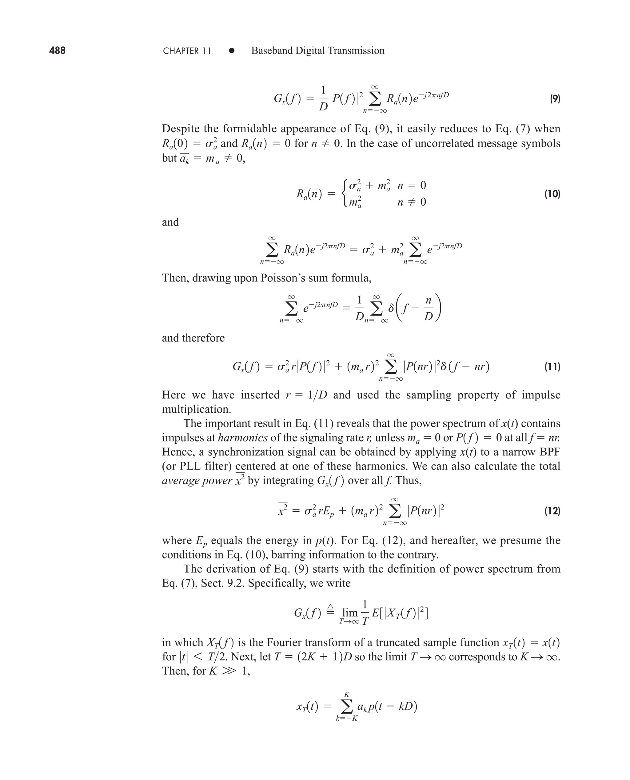
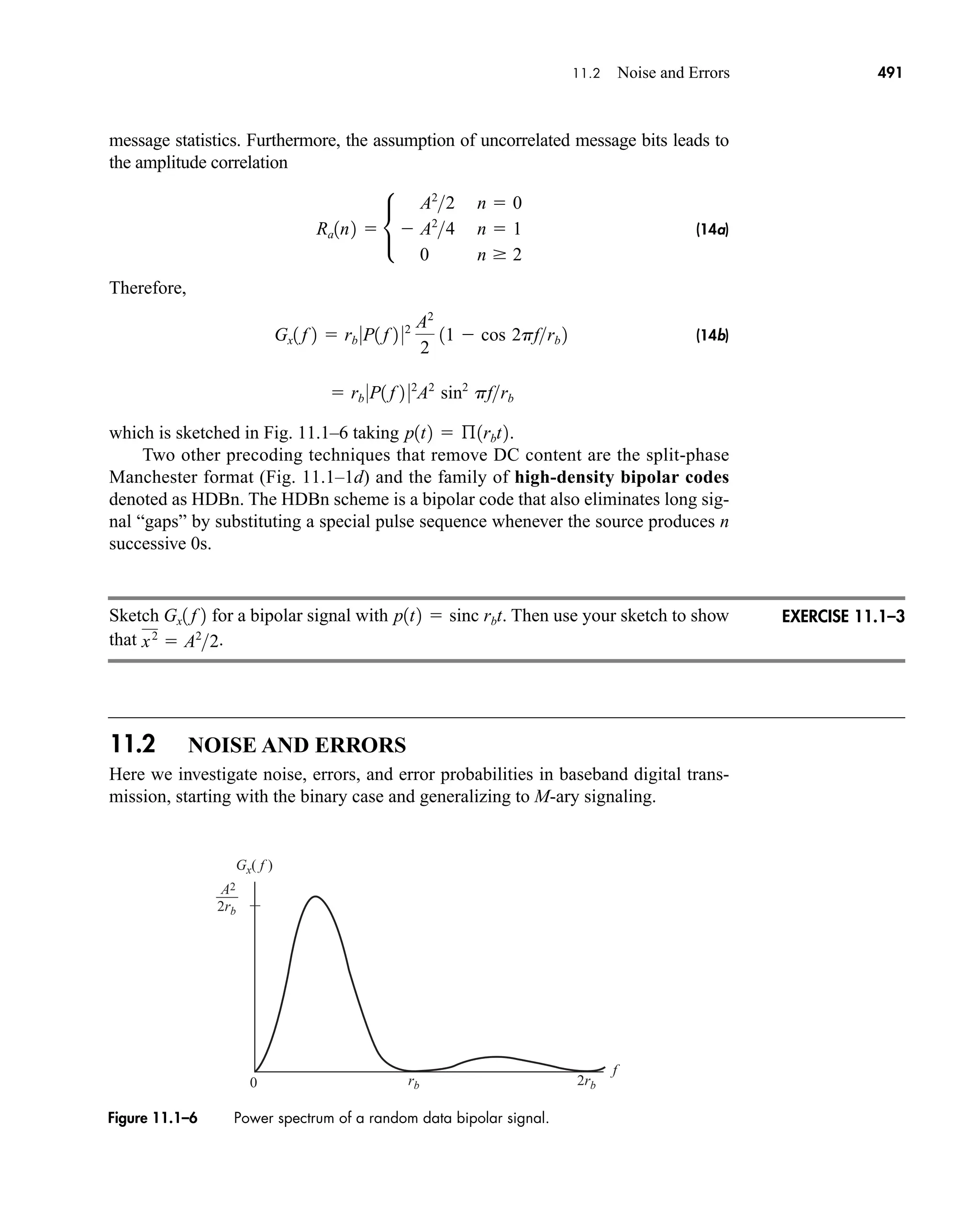
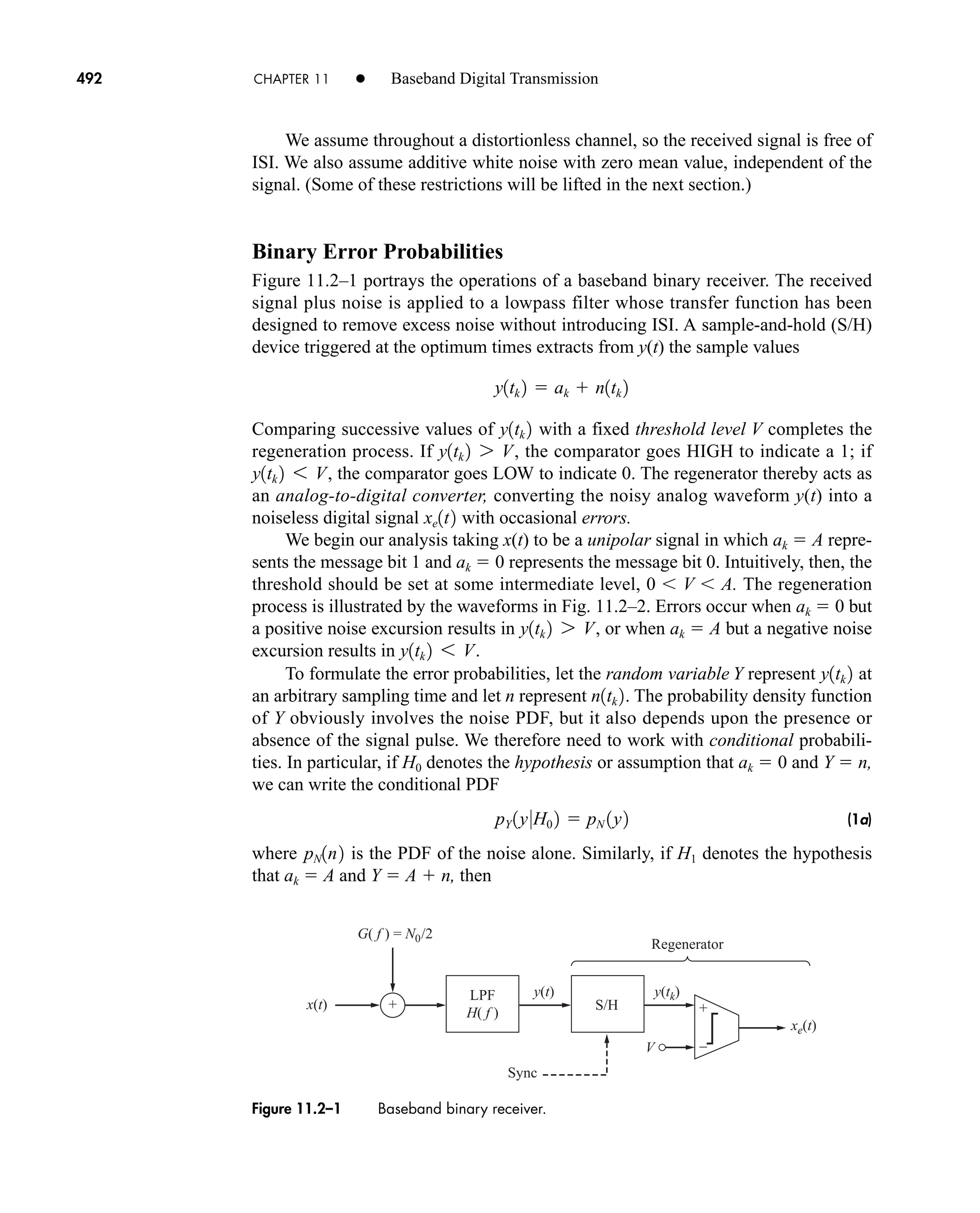
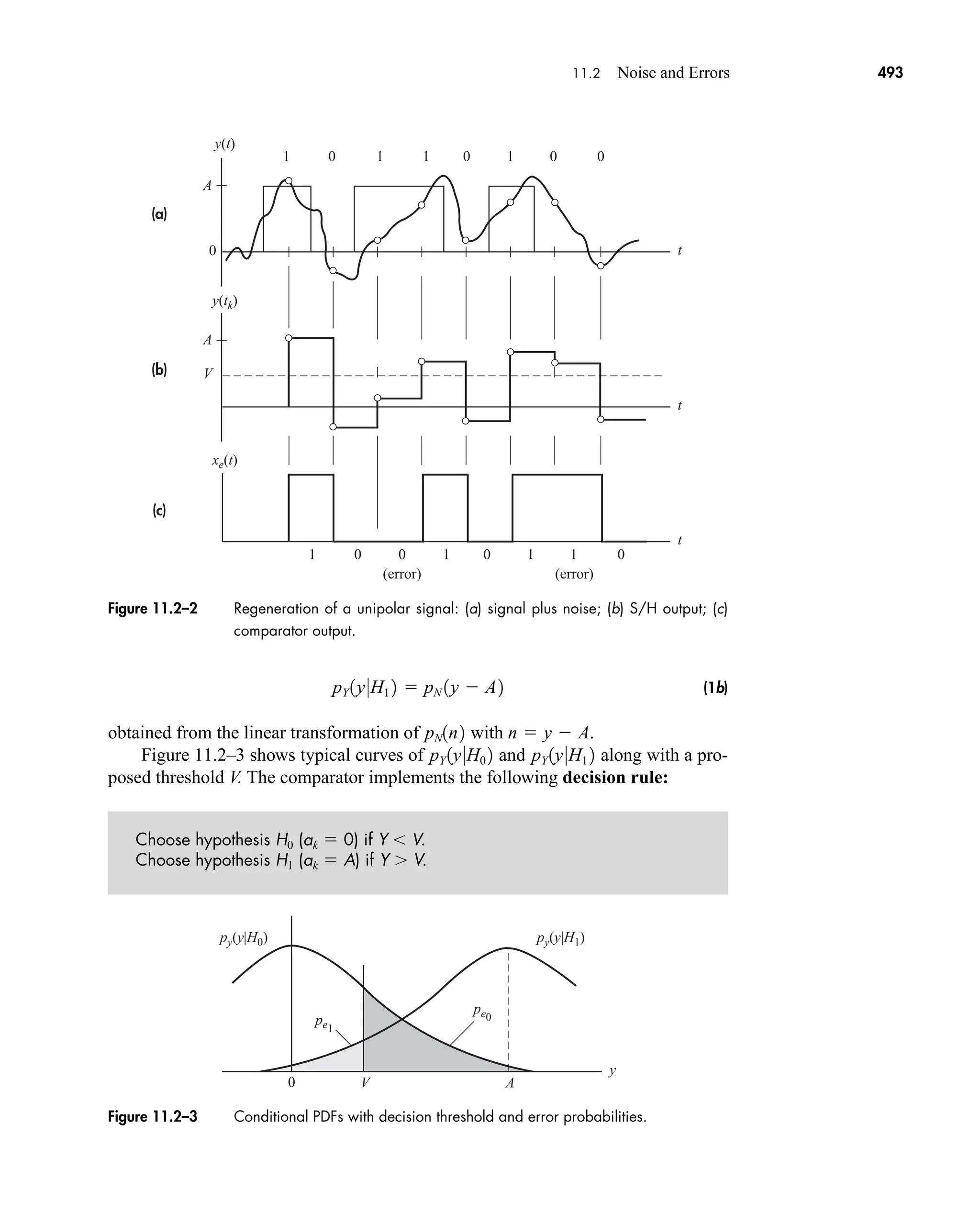
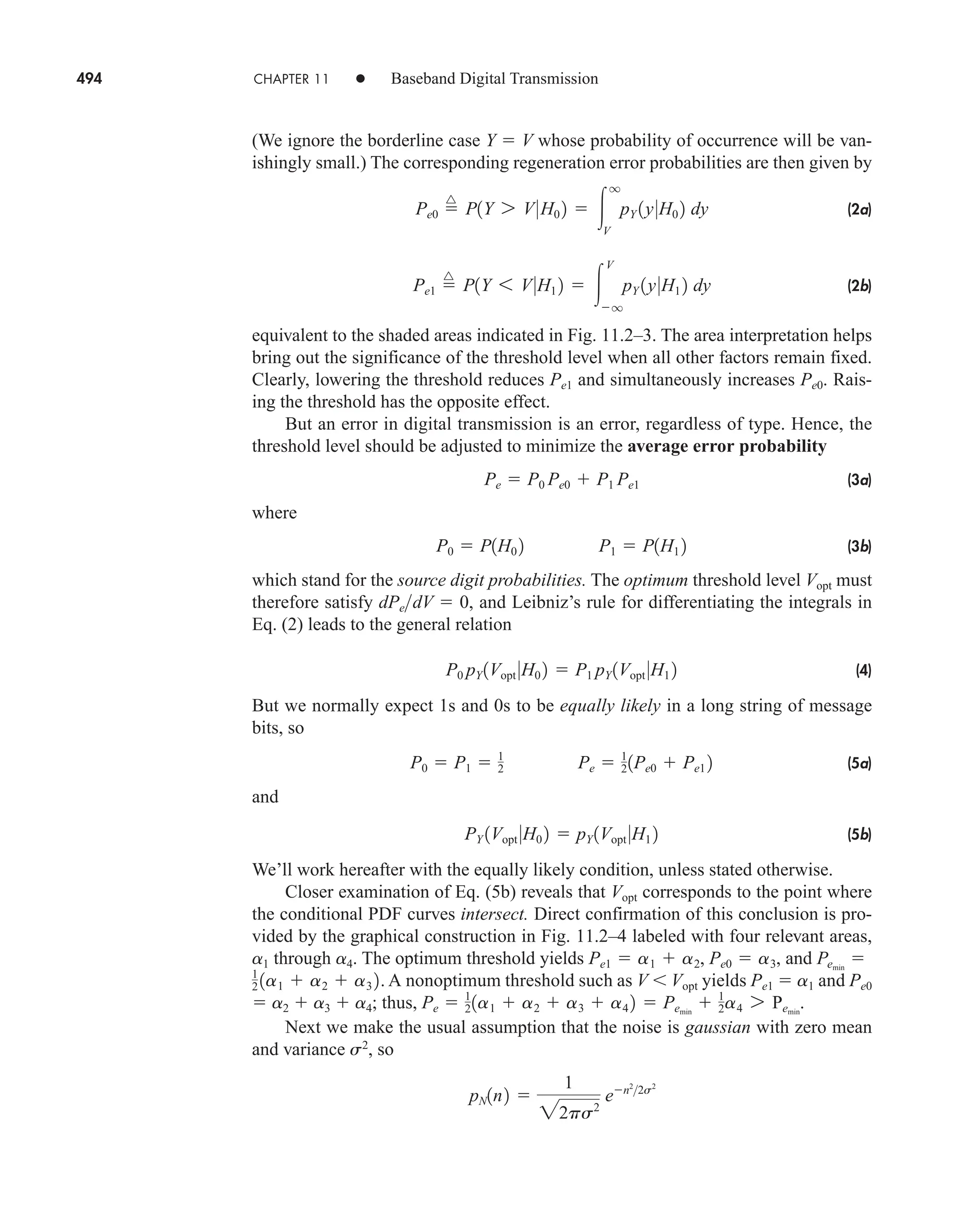
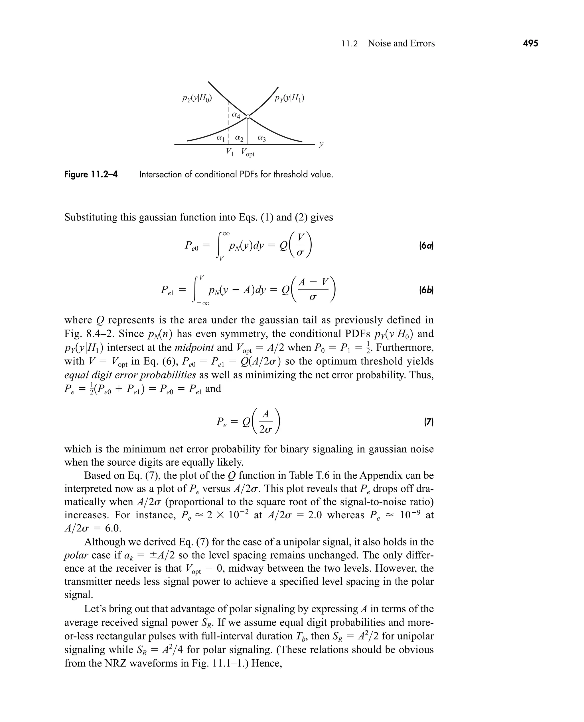
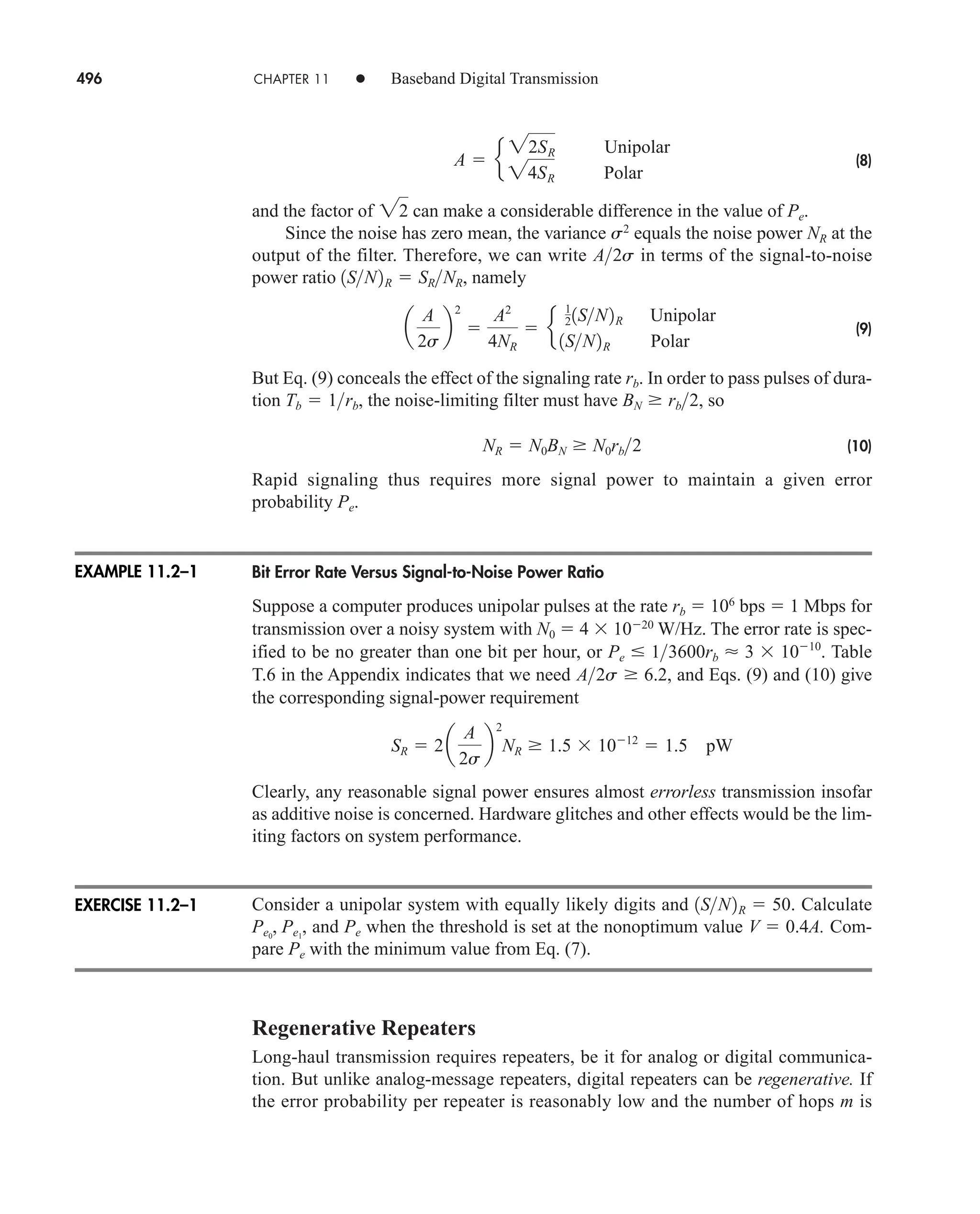
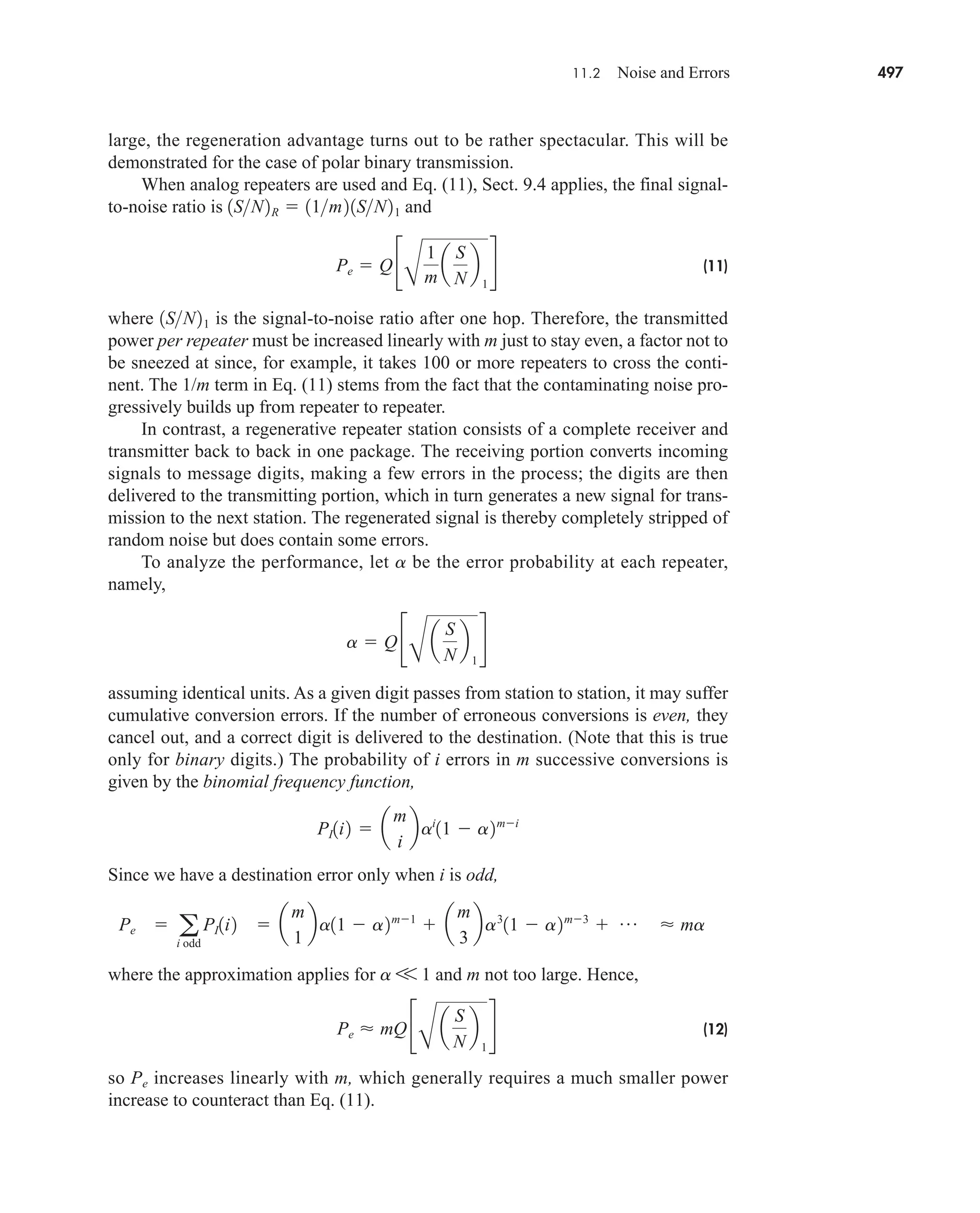
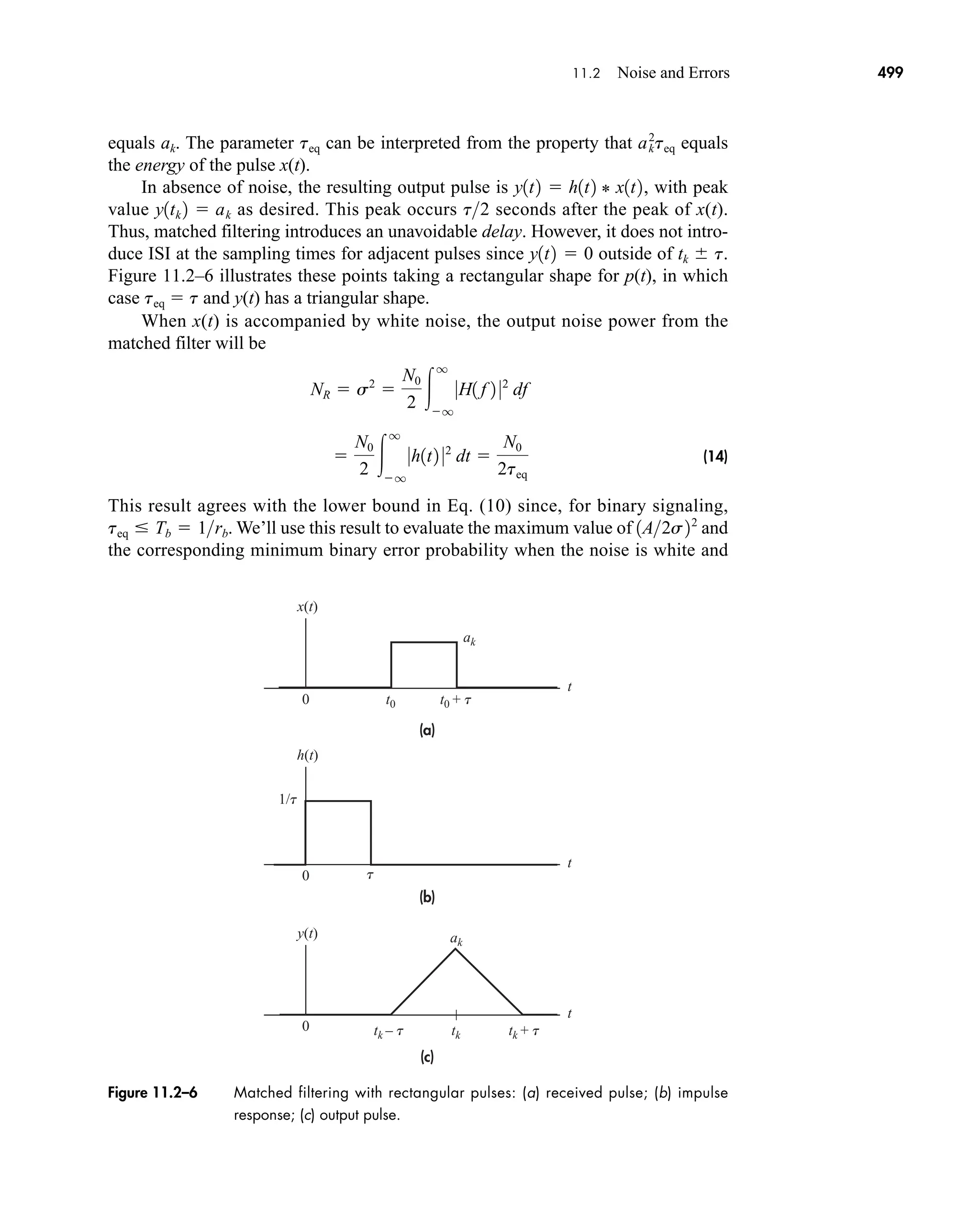
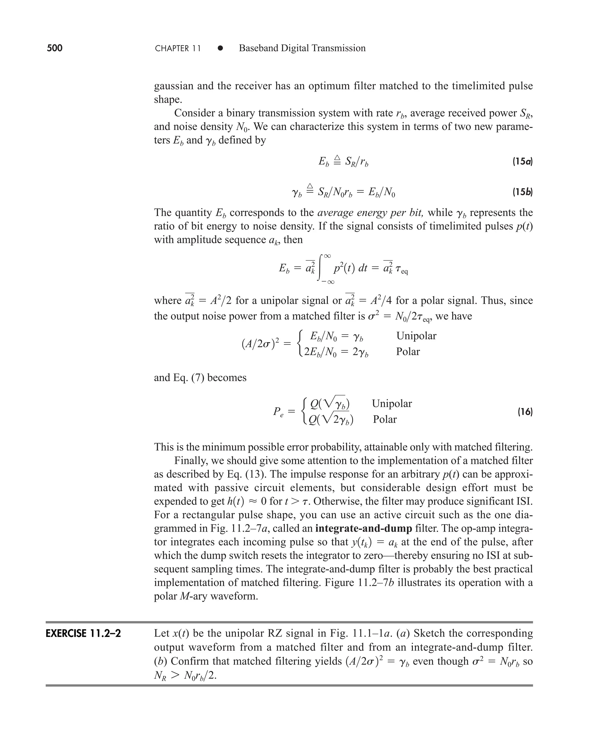
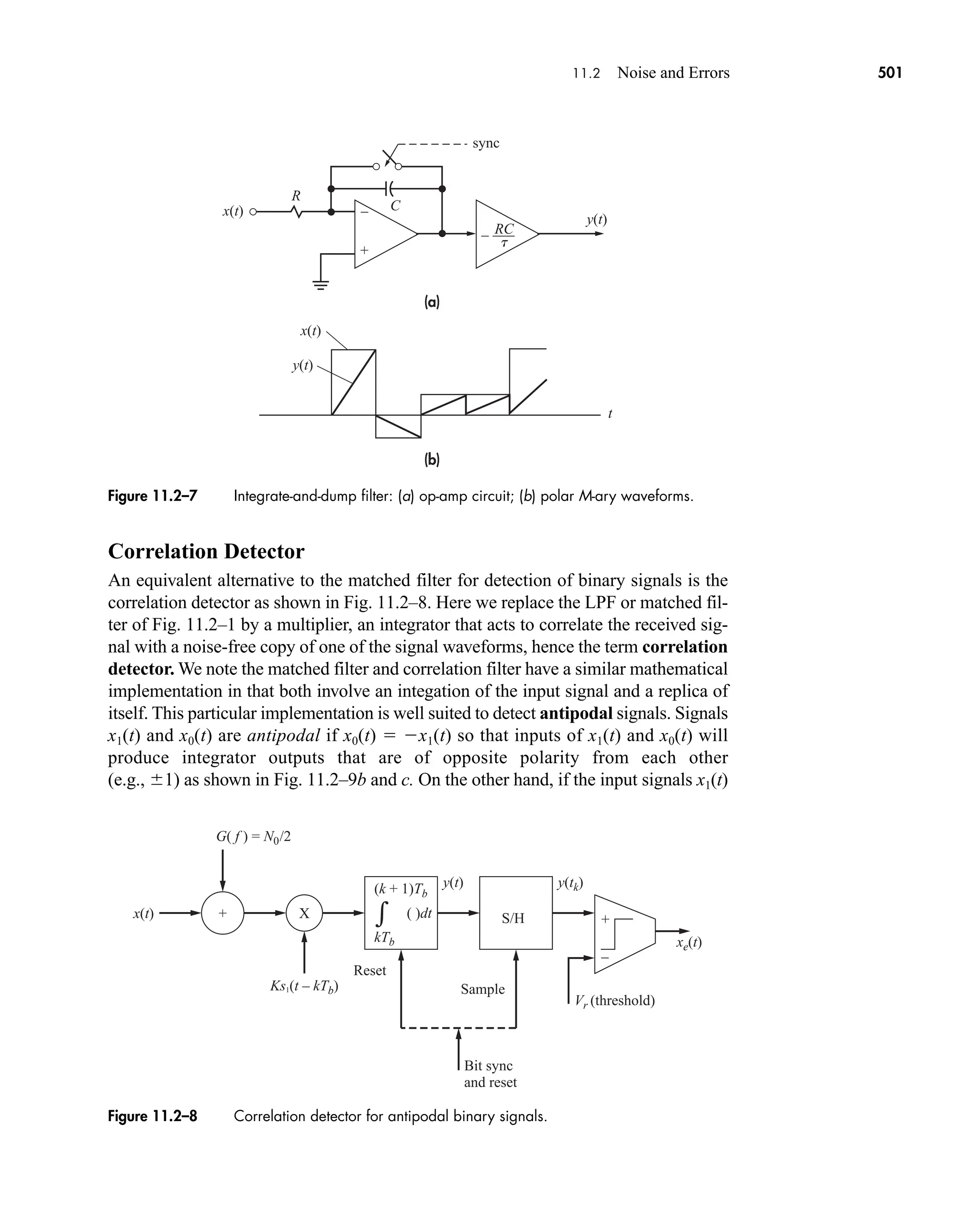
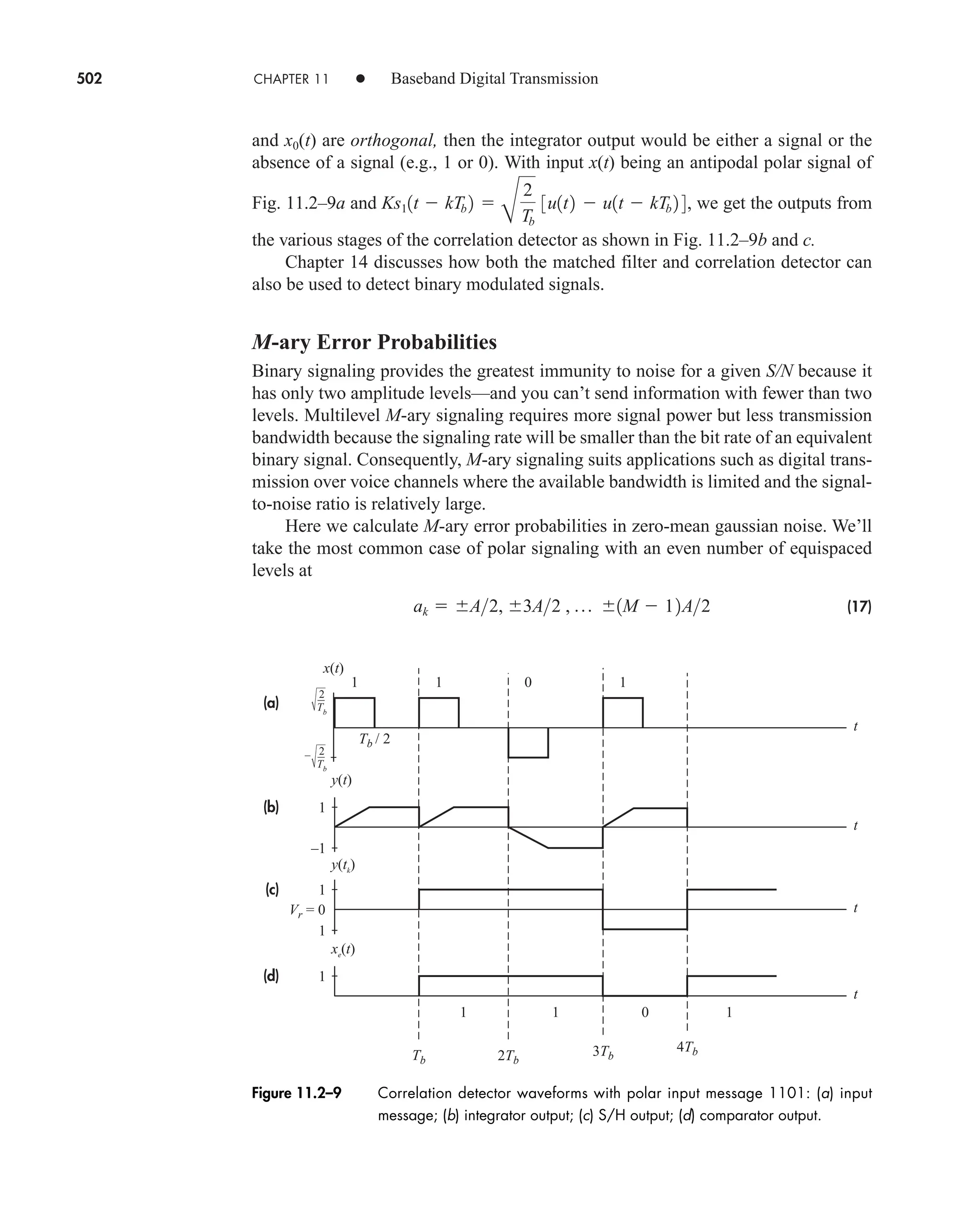
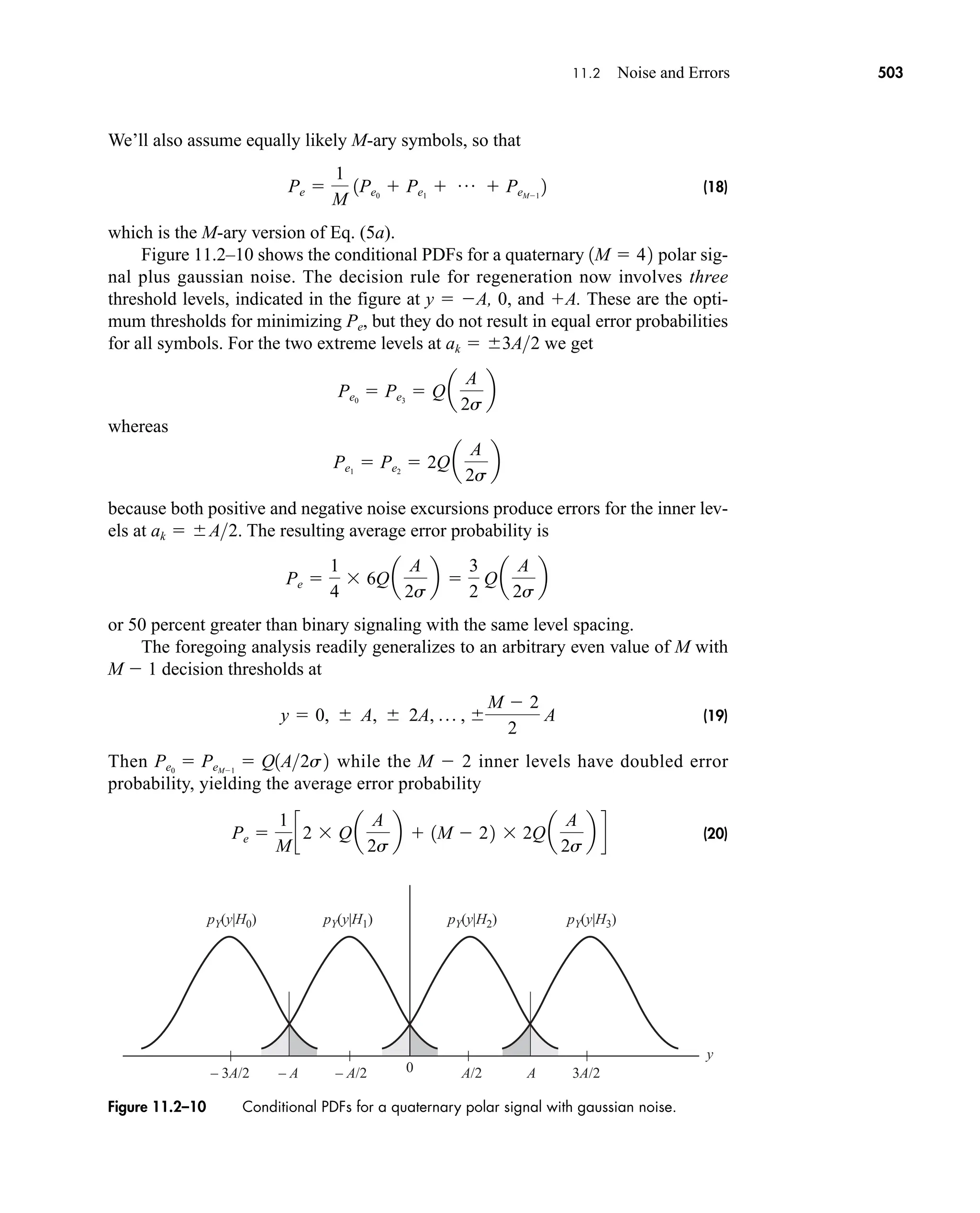
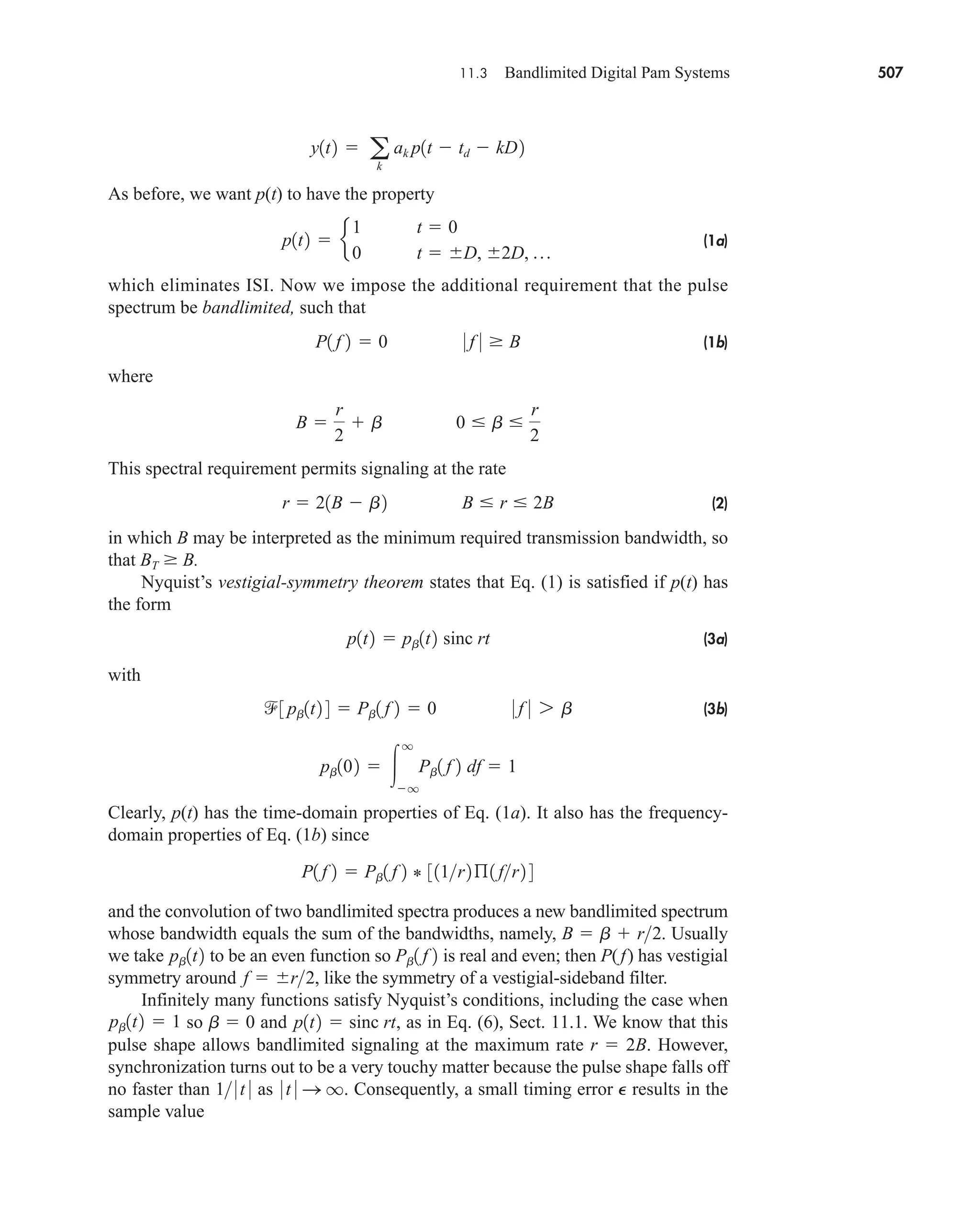
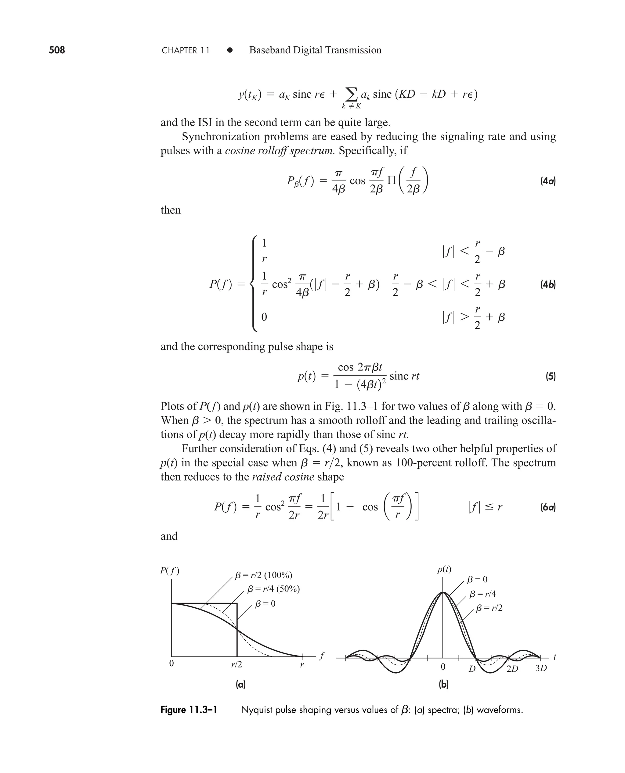
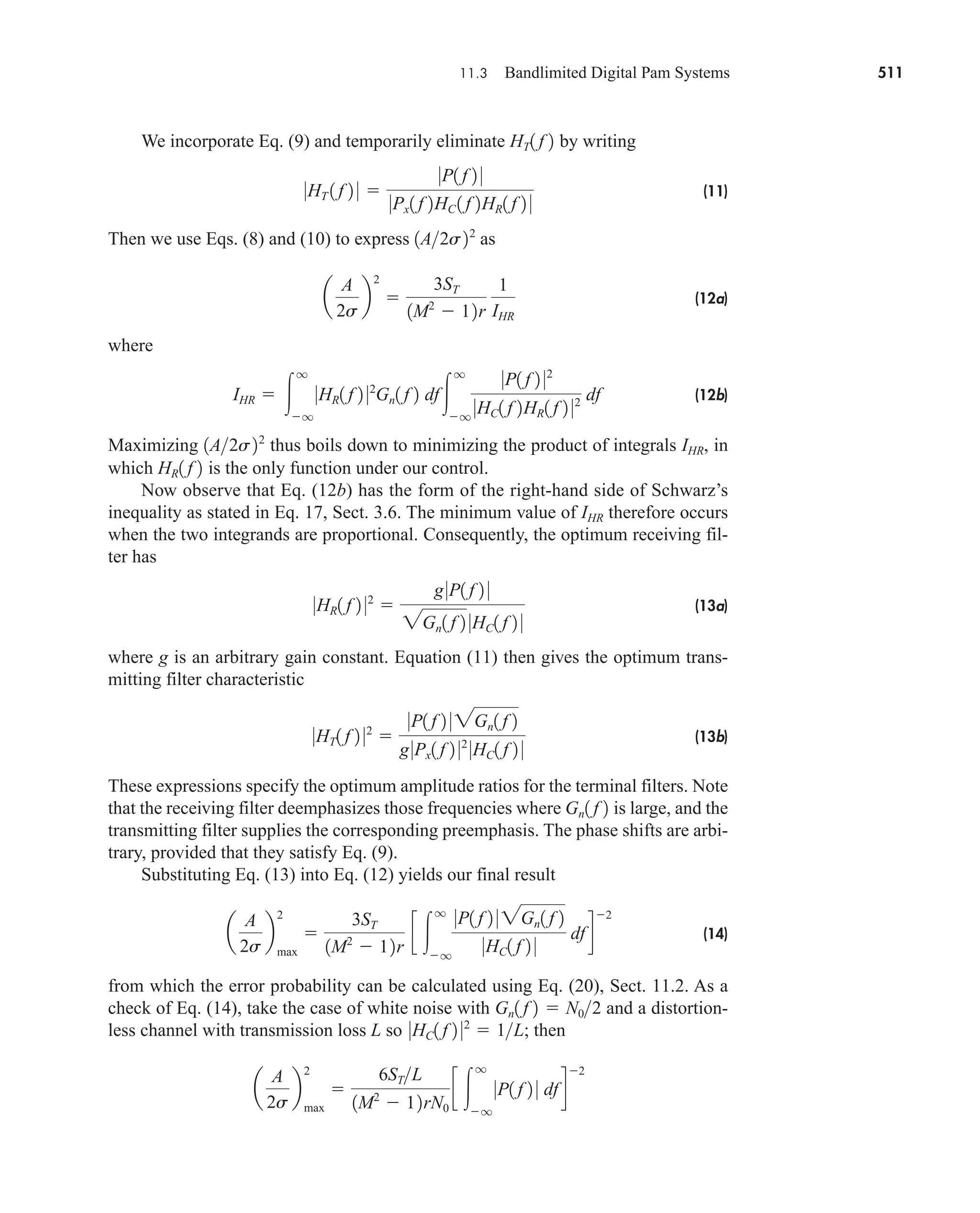
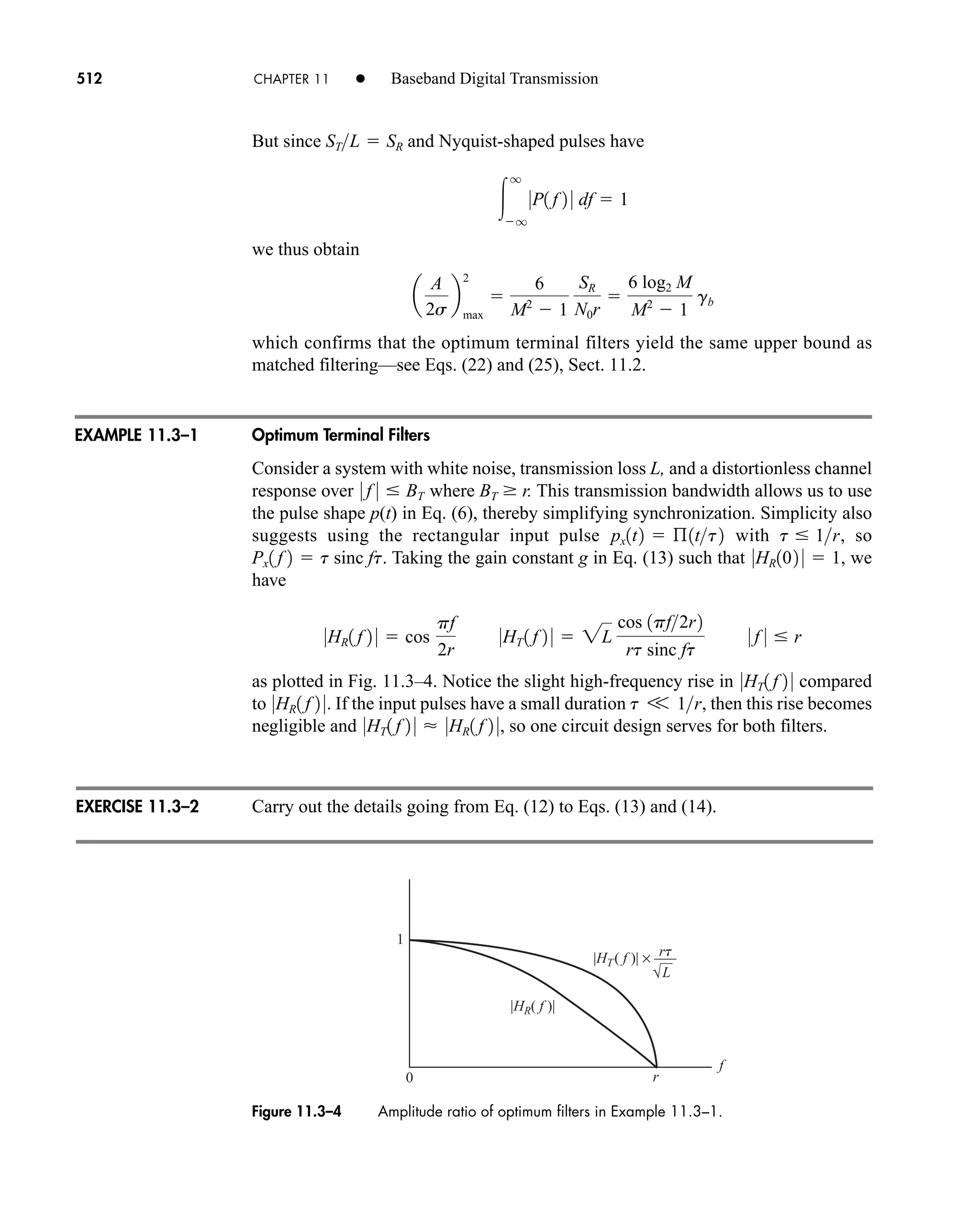
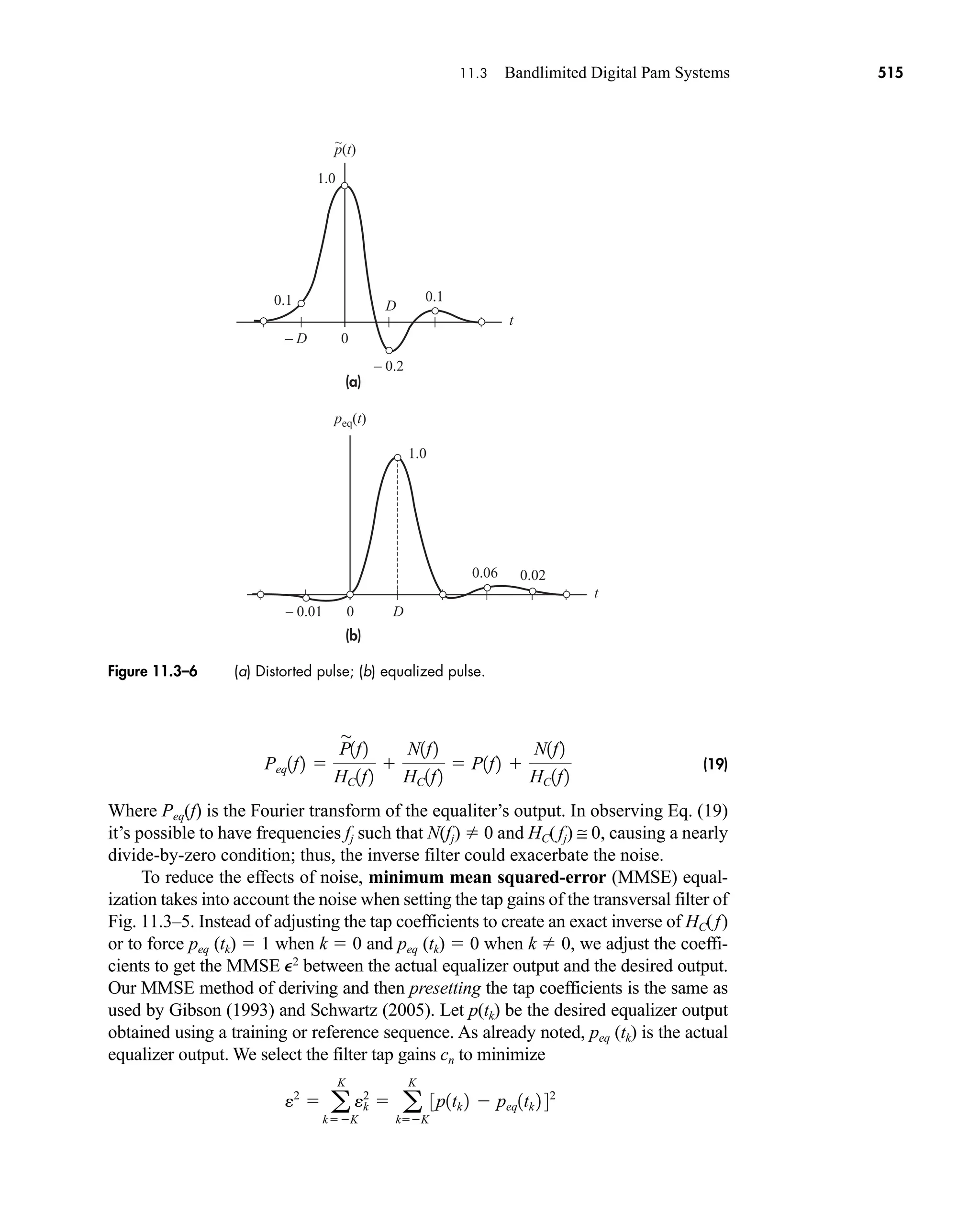
![516 CHAPTER 11 • Baseband Digital Transmission
(20)
with cm the particular coefficient we want to calculate. To get the MMSE we take the
partial derivative of Eq. (20) with respect to cm, setting it to zero, and then we get
(21)
Note, in taking the derivative with respect to cm, that cm is the coefficient for
Rearranging terms, Eq. (21) becomes
and then
(22)
To implement Eq. (22), we will use the [0,0 . . 1, 0, 0. . . 0] output of Eq. (17) to obtain
p(tk). The unqualized signal samples are obtained by measuring the filter outputs.
As you will observe in doing Probs. 11.3–20 and 11.3–21, using Eq. (17) to get p(tk)
for Eq. (22) is not the same as implementing the zero forcing algorithm previously
discussed. With 2N 1 equations and 2N 1 unknowns we can then compute the
2N 1 tap coefficients. Also, when setting up the terms of Eq. (22), each of the
2N 1 equations corresponds to a fixed value of m. For example, let’s say we want to
implement a three-tap equalization filter of Example 11.3–2; Eq. (22) is set up as follows
(Gibson, 1993):
The ci coefficients are then obtained by solving the above equations using the given
values of , and p(tk). An alternative approach to this MMSE method discussed
in the literature uses the signal’s autocorrelation and cross-correlation statistics.
During the transmission, the channel characteristics may vary, and it would be
desirable to have the filter track these changes in order to update the coefficients and
thus create an adaptive equalizer. This can work if the channel is a switched telephone
link or some other path with slowly changing conditions. The reference signal p(tk)
p
'
k , p
'
k ; 1
c1 a
k
p
'
k1p
'
k1 c0 a
k
p
'
k p
'
k1 c1 a
k
p
'
k1
2
a
k
p1tk 2p
'
k1
m 1
c1 a
k
p
'
k1p
'
k c0 a
k
p
'
k
2
c1 a
k
p
'
k1p
'
k a
k
p1tk 2p
'
k
m 0
c1 a
k
p
'
k1
2
c0 a
k
p
'
k p
'
k1 c1 a
k
p
'
k1 p
'
k1 a
k
p1tk 2p
'
k1
m 1
p
'
kn
a
N
nN
cn a
K
kK
p
'
kn˛
p
'
km a
K
kK
p1tk 2p
'
km
a
K
kK
a
N
nN
cn p
'
kn˛p
'
km a
K
kK
p1tk 2p
'
km
p
'
km .
0e2
0cm
0 2 a
K
kK
cp1tk 2 a
N
nN
cn p
'
kn dp
'
km
a
K
kK
cp1tk 2 a
N
nN
cn p
'
kn d
2
car80407_ch11_479-542.qxd 9/1/09 9:55 AM Page 516](https://image.slidesharecdn.com/communicationsystemsanintro-a-241115060943-61721fa8/75/Communication_Systems__An_Intro_-_A-_Bruce_Carlson_-pdf-538-2048.jpg)
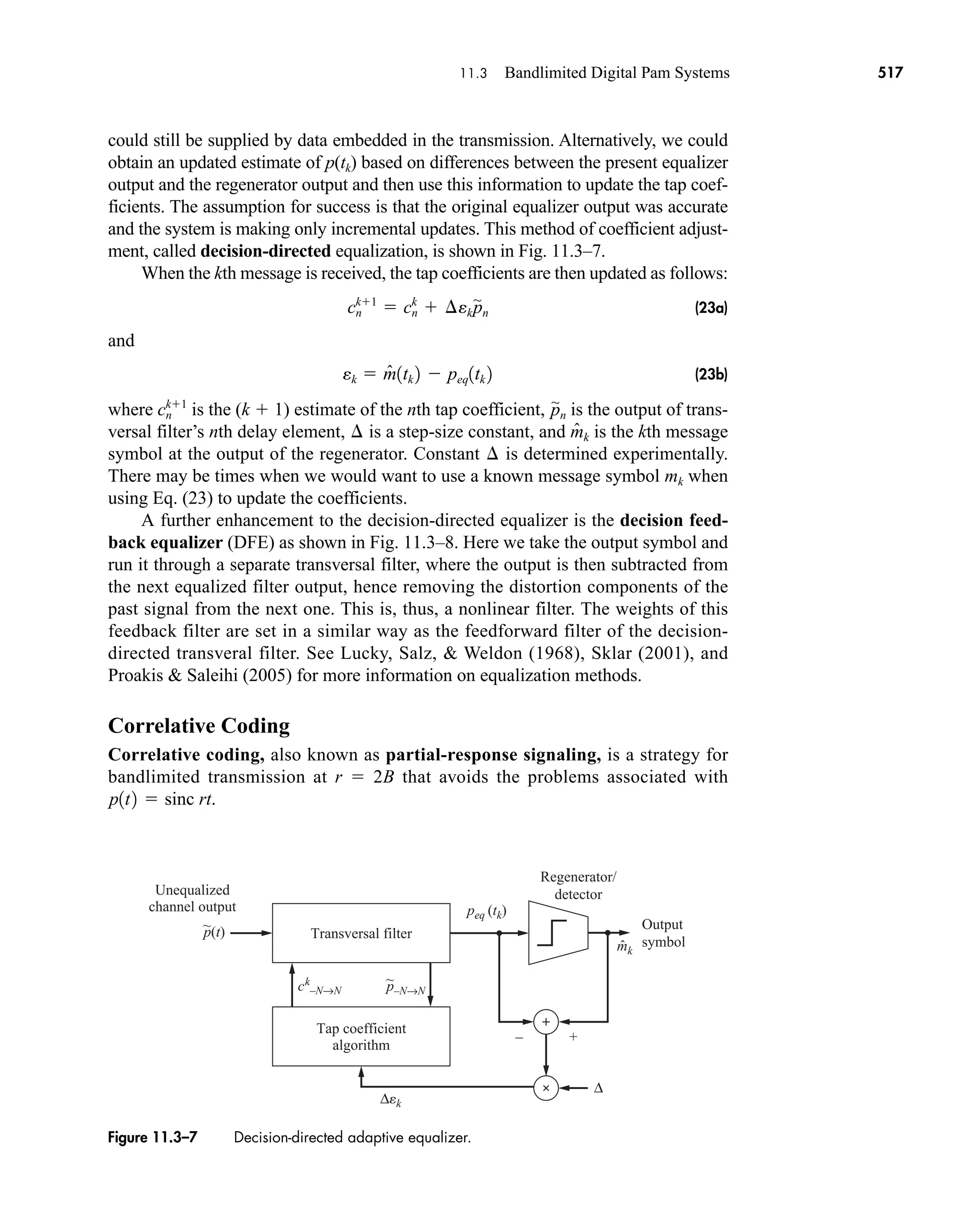
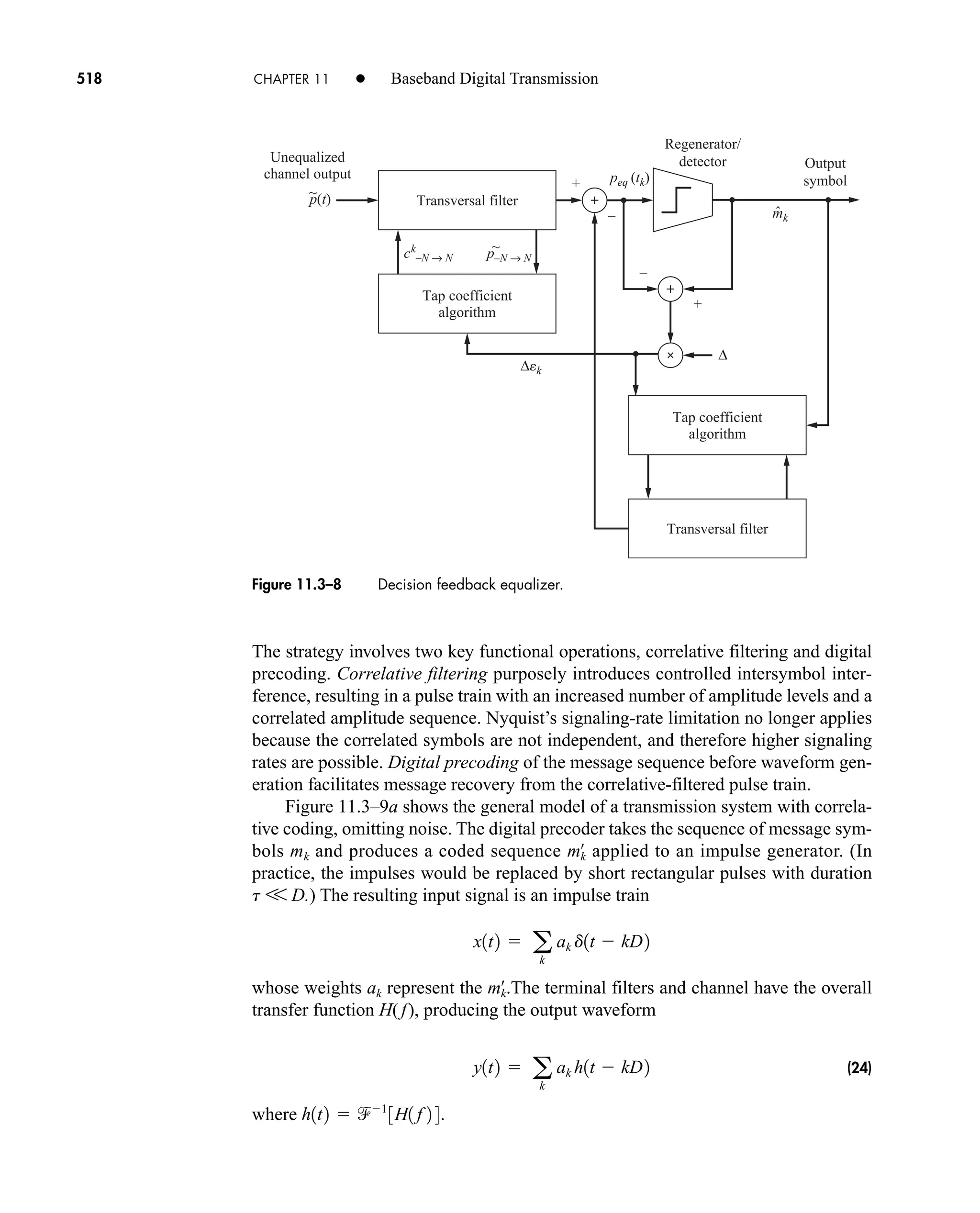
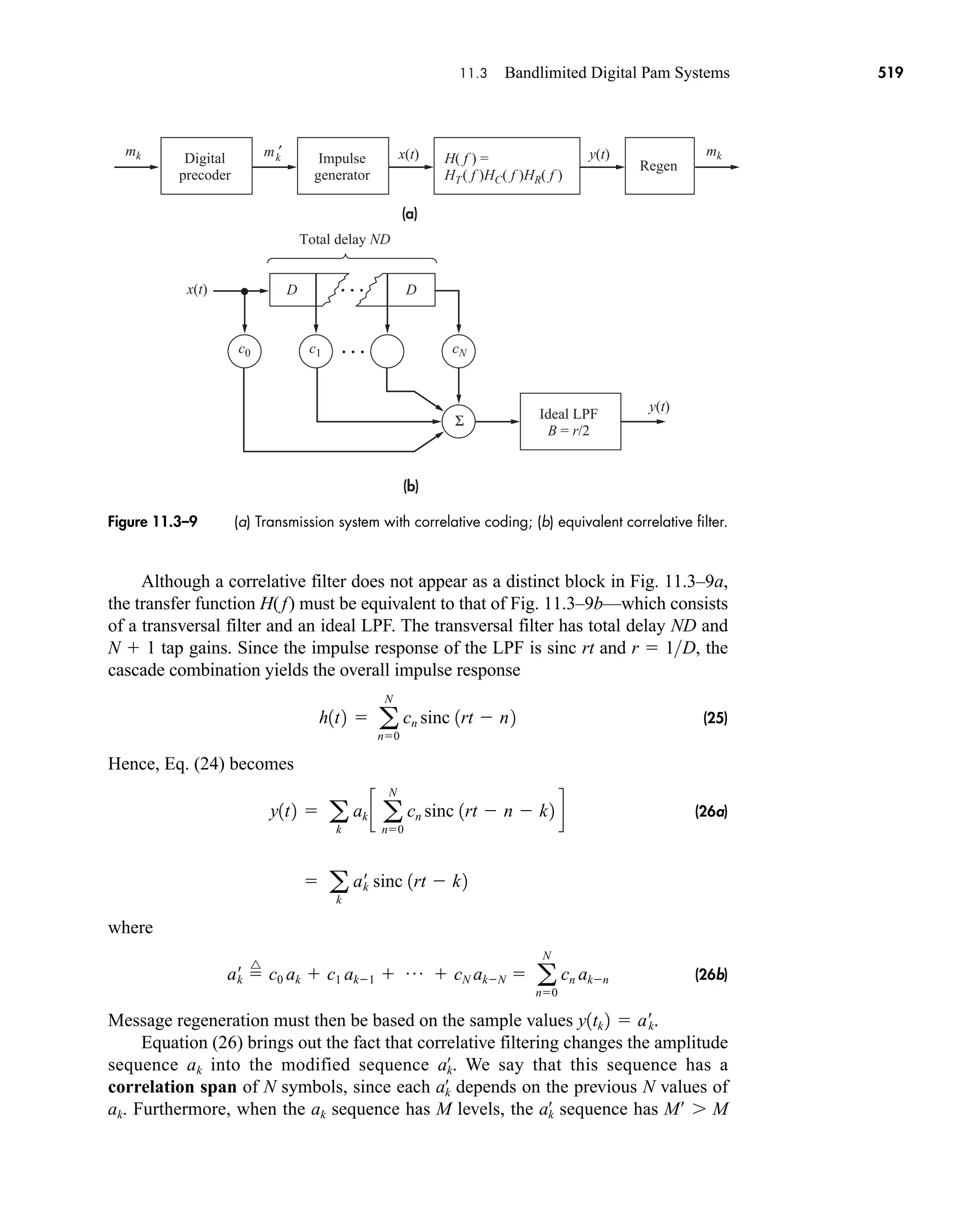
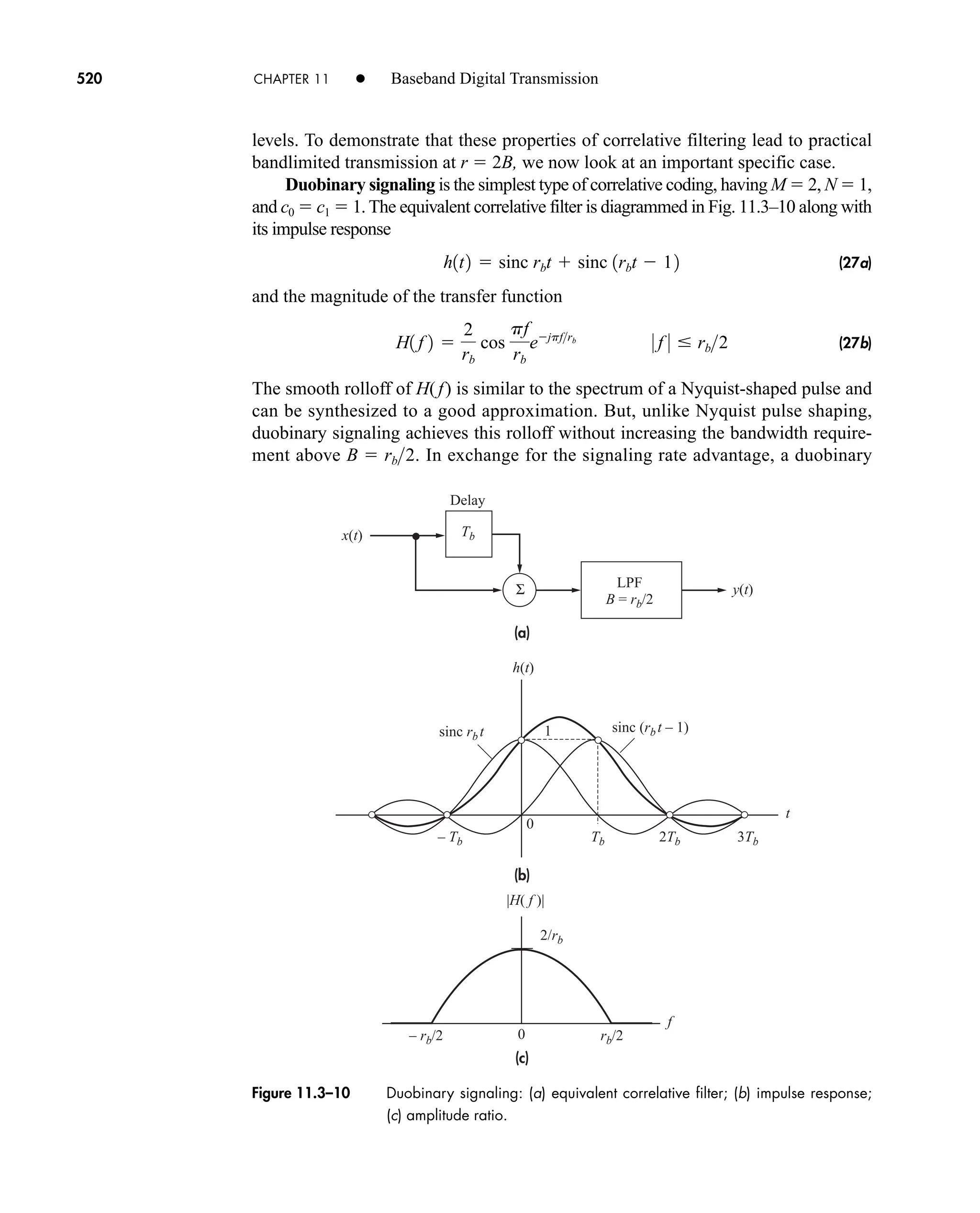
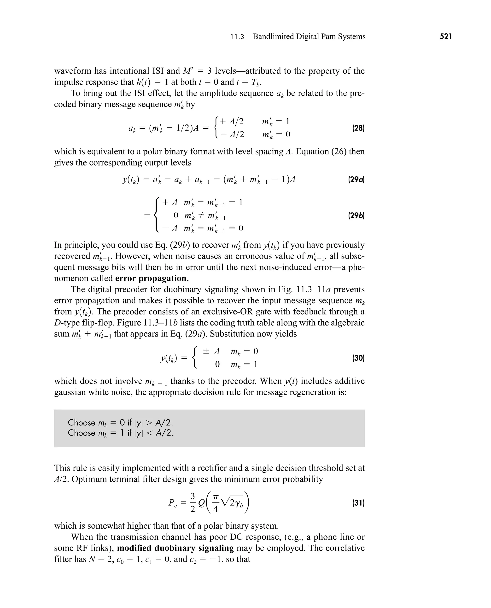
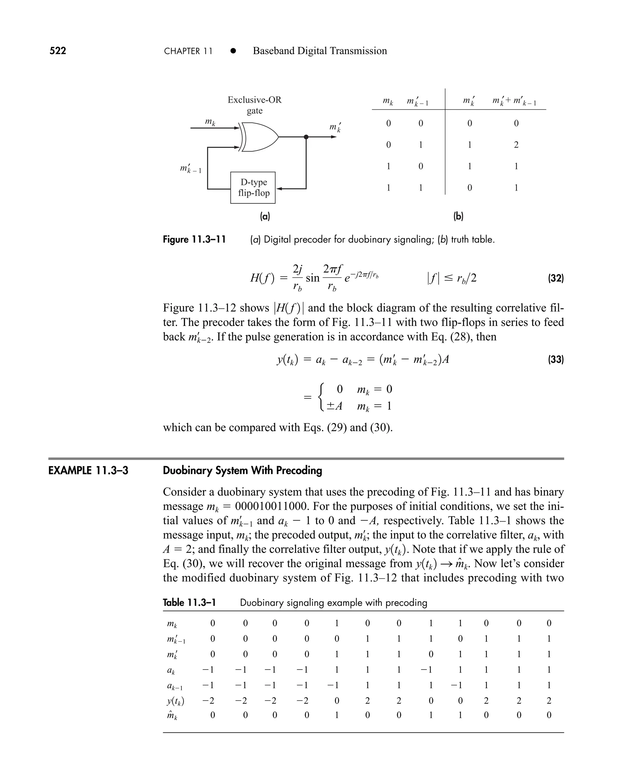
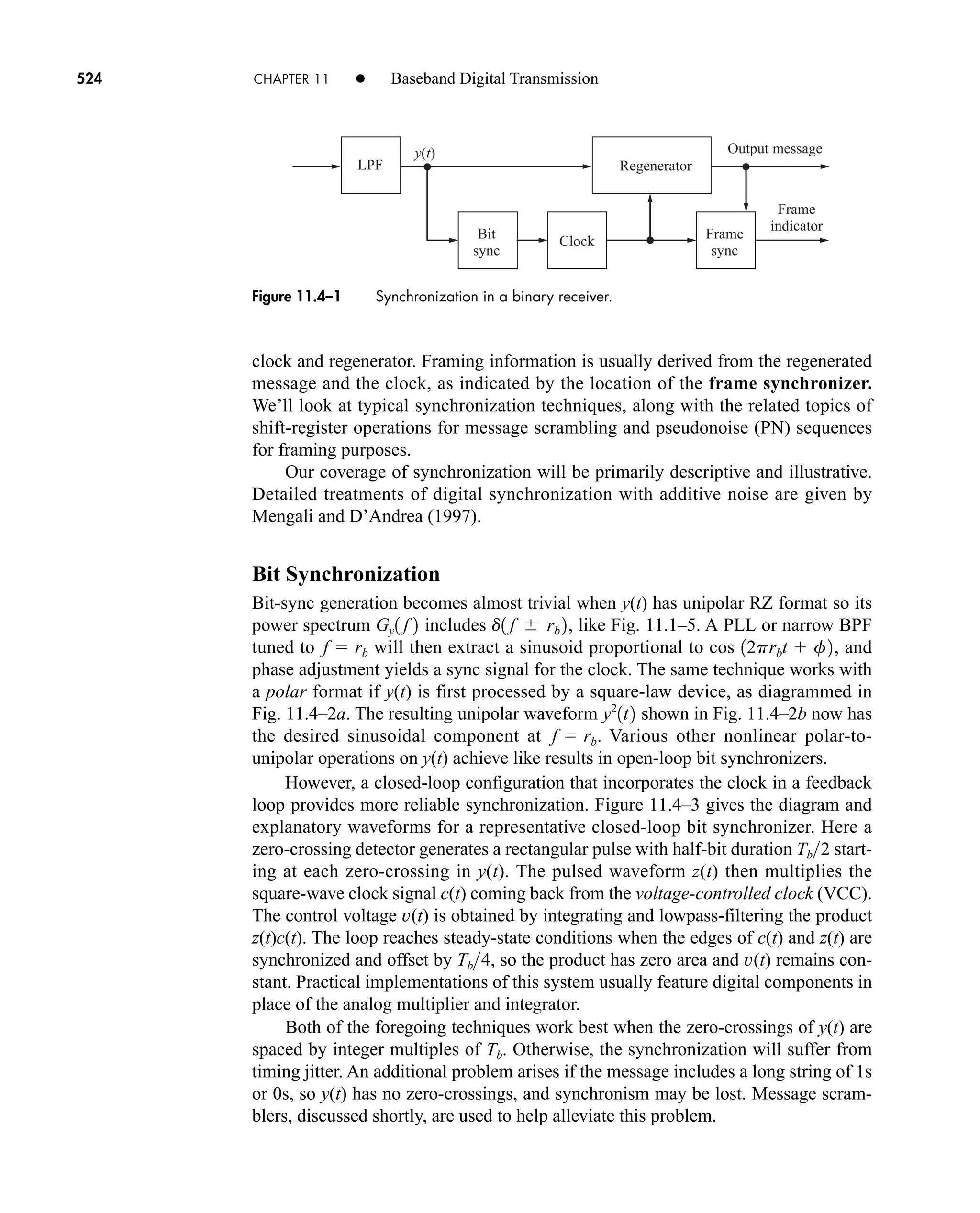
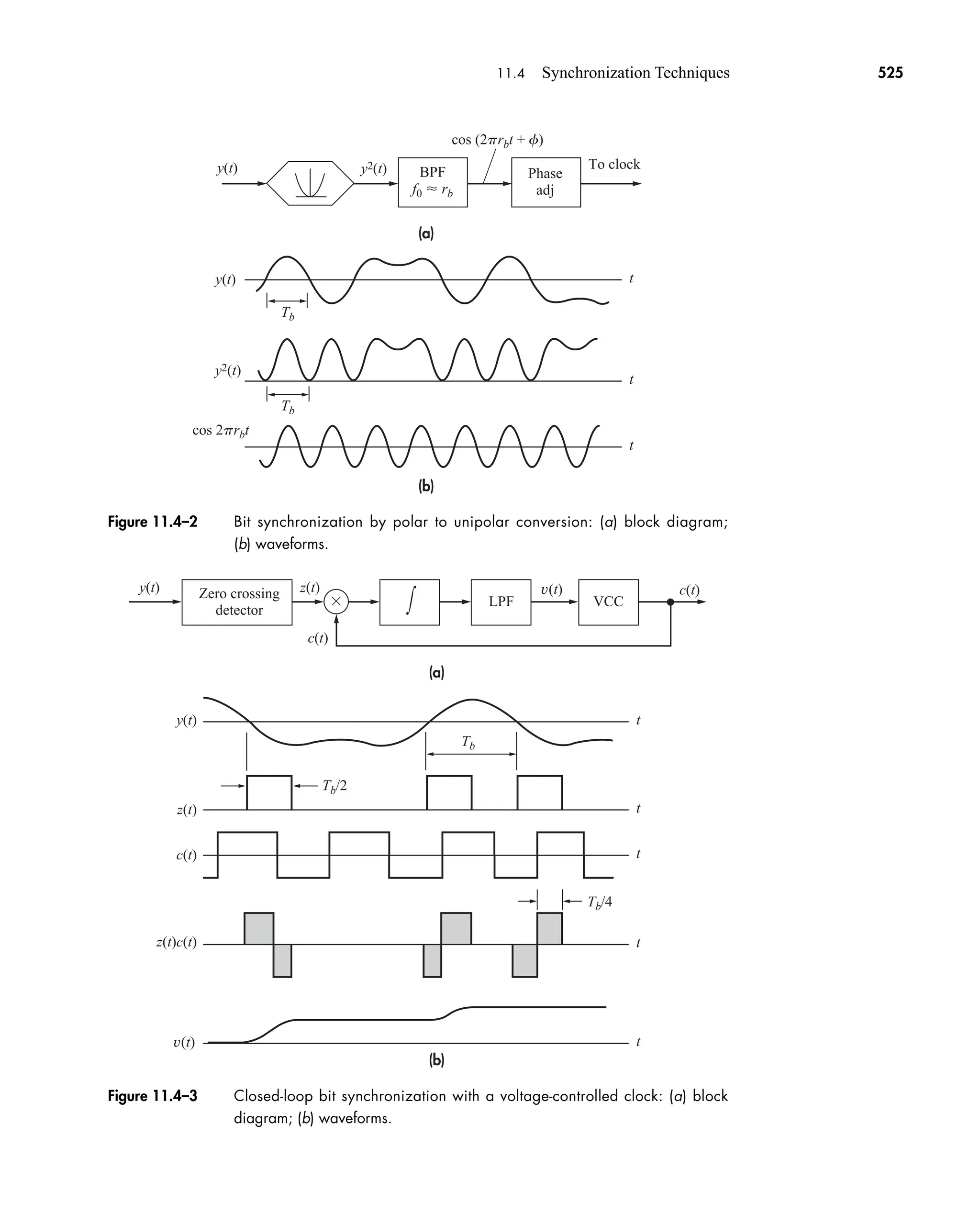
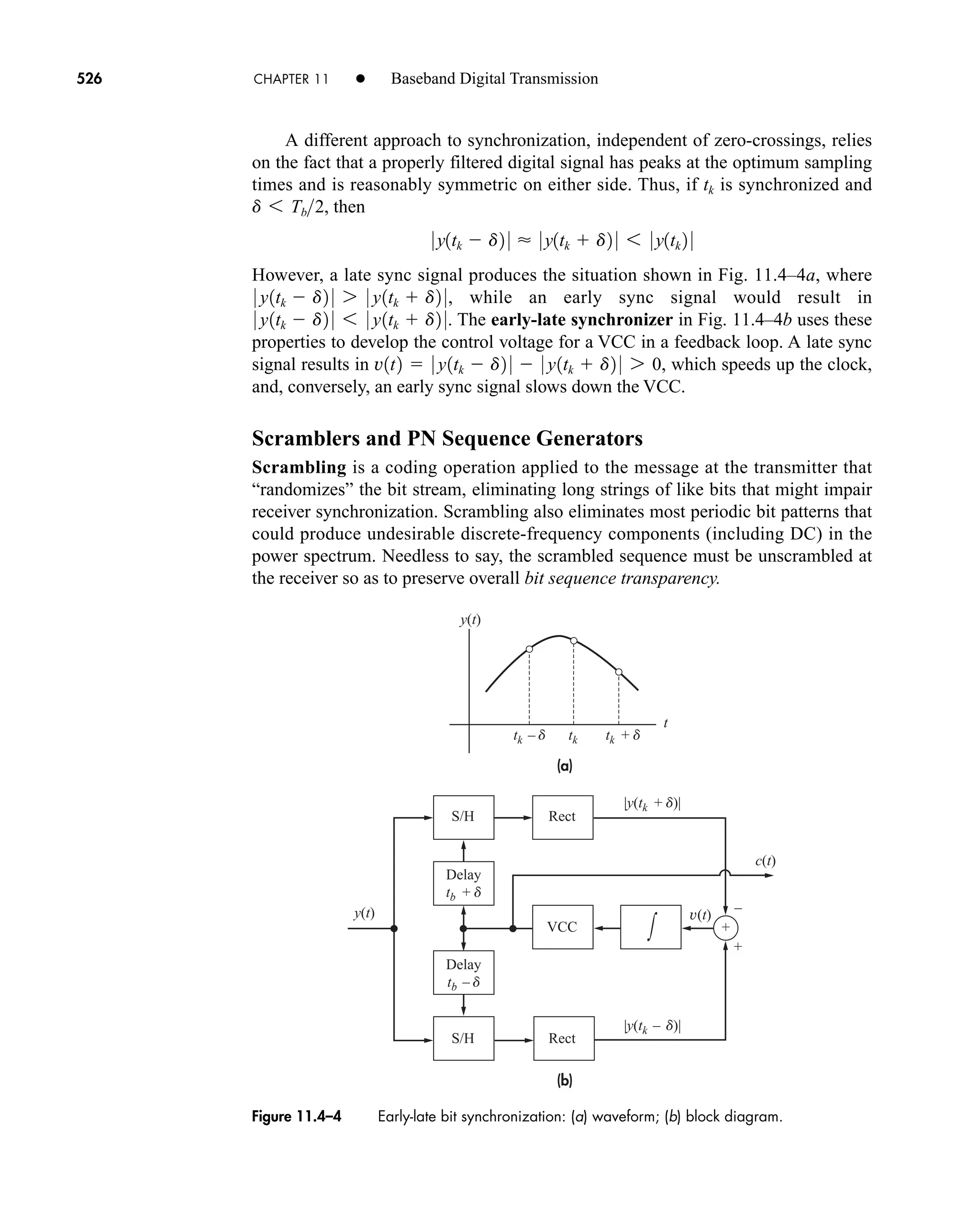
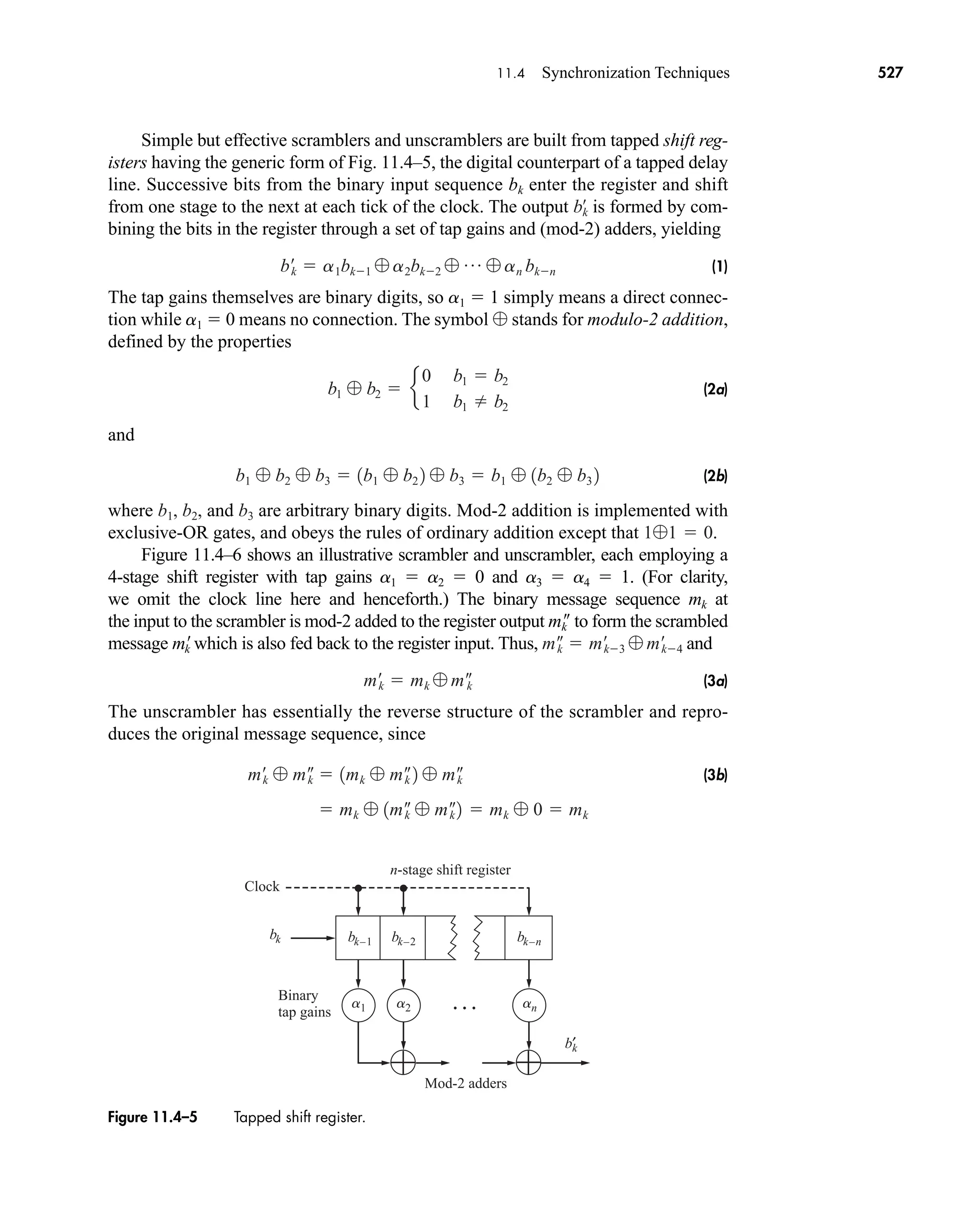
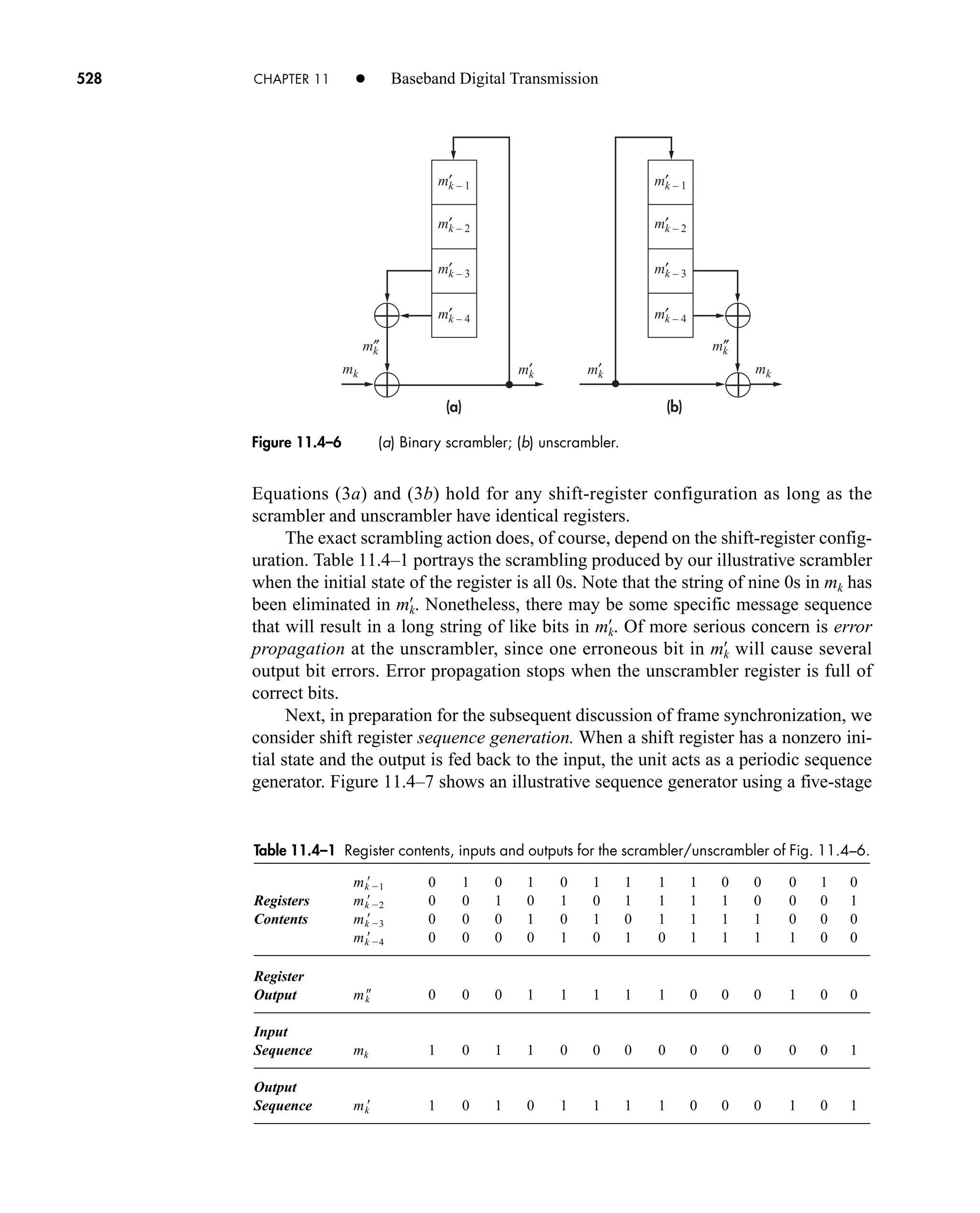
![+
m1
1
m2
1
m3
1
Output sequence
111010...
m4
1
m5
1
Figure 11.4–7 Shift register sequence generator with [5, 2] configuration.
11.4 Synchronization Techniques 529
shift register where the second and fifth cells are tapped and mod-2 added, and the
result is fed back to the first stage so
(4)
and the sequence output is m5. For shorthand purposes this can also be referred to as
a [5, 2] configuration. If the initial state of the register is 11111, it then produces a
31-bit sequence 1111100110100100001010111011000, which repeats periodically
thereafter. In general
(5)
If the appropriate feedback tap connections are made, then an n-bit register can
produce a maximal-length (ML) sequence per Eq. (5). (Figure 11.4–7 is, in fact, an
ML sequence generator with n 5 and N 31.) An ML sequence has the following
properties:
1. Balance. The number of ones generated is one more than the number of zeros
generated.
2. Run. A run is a sequence of a single type of digit. An ML sequence will have
one-half of its runs of length 1, one-quarter of its runs of length 2, one-eighth of
its runs of length 3, and so on.
3. Autocorrelation. Its autocorrelation function has properties similar to the corre-
lation properties of random noise, in that there is a single autocorrelation peak.
4. The mod-2 addition of an ML sequence and any shifted version of it results in a
shifted version of the original sequence.
5. Except for the zero state, all of the 2n
possible states will exist during the
sequence generation.
Maximal-length sequences are all also called pseudonoise (PN) sequences. The
name pseudonoise comes from the correlation properties of PN sequences. To
develop this point, let a PN sequence sk be used to form a binary polar NRZ signal
(6)
where p(t) is a rectangular pulse and the amplitude of the kth pulse is
(7)
c1t2 2sk 1 e
1 sk 1
1 sk 0
s1t2 a
k
12sk 12p1t kTc 2
N 2n
1
m1 m2 m5
car80407_ch11_479-542.qxd 12/17/08 6:35 PM Page 529
Confirming Pages](https://image.slidesharecdn.com/communicationsystemsanintro-a-241115060943-61721fa8/75/Communication_Systems__An_Intro_-_A-_Bruce_Carlson_-pdf-551-2048.jpg)
 v(T)/N
0 1110100 7.00 1.00
1110100
1 1110100 1.00 0.14
0111010
2 1110100 1.00 0.14
0011101
3 1110100 1.00 0.14
1001110
4 1110100 1.00 0.14
0100111
5 1110100 1.00 0.14
1010011
6 1110100 1.00 0.14
1101001
0 1110100 7.00 1.00
1110100
530 CHAPTER 11 • Baseband Digital Transmission
The signal s(t) is deterministic and periodic, with period NTc, and has a periodic
autocorrelation function given by
(8)
which is plotted in Fig. 11.4–8. If N is very large and Tc very small, then
(9)
so the PN signal acts essentially like white noise with a small DC component. This
noiselike correlation property leads to practical applications in test instruments, radar
ranging, spread-spectrum communications (described in Chap. 15), and digital framing.
When we do use PN generators to operate on a data stream, to avoid significant DC con-
tent in the PN sequence and minimize information loss to the signal we are operating
on, we use the function c(t) instead of the polar for our scrambling sequence.
Autocorrelation of a [3,1] Shift Register
A 3-bit, [3, 1] shift register configuration with values of 111 produces a periodic ML
sequence of 1110100 with N 7. A simple way used by Dixon (1994) to calculate
the autocorrelation function for the comparable c(t) sequence is to compare the orig-
inal sk sequence to each of its N 1 shifted versions (t 0 to 6Tc). Then, for each
pair, let v(t) be the difference between the number of bit matches and mismatches,
so the autocorrelation function is and hence the results shown in
Table 11.4–2.
R33, 141t2 v1t2N
sk
Rs1t2 Tcd1t2 1N 0t0 NTc2
Rc1t2 31N 12¶1tTc 2 14N 0t0 NTc2
EXAMPLE 11.4–1
car80407_ch11_479-542.qxd 12/17/08 6:35 PM Page 530
Confirming Pages](https://image.slidesharecdn.com/communicationsystemsanintro-a-241115060943-61721fa8/75/Communication_Systems__An_Intro_-_A-_Bruce_Carlson_-pdf-552-2048.jpg)