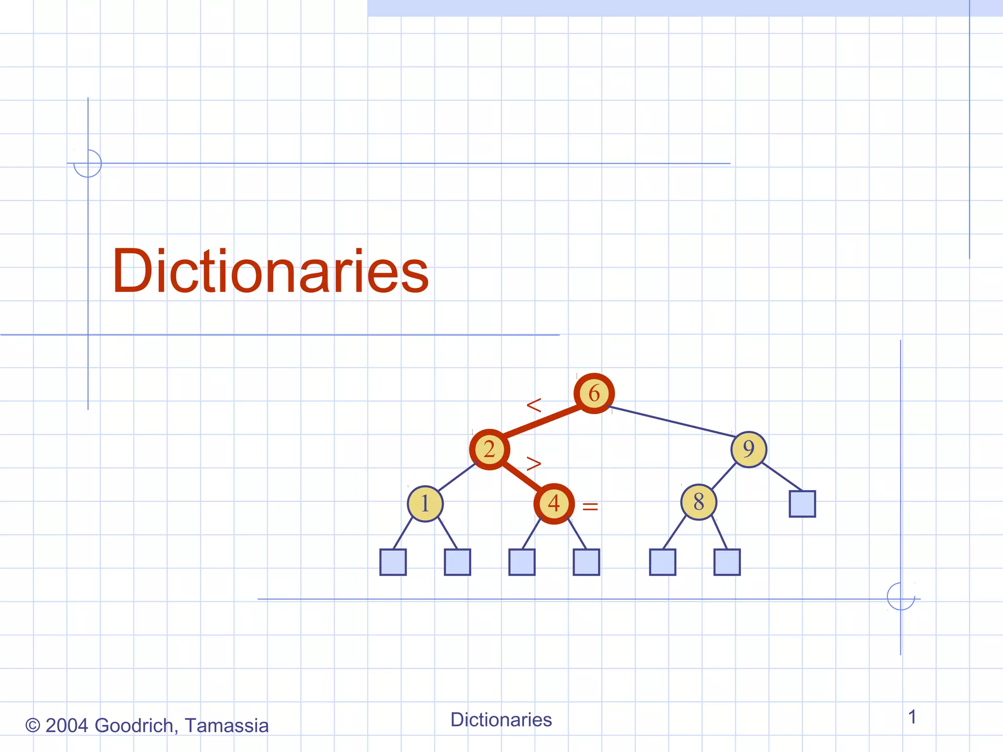
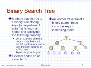
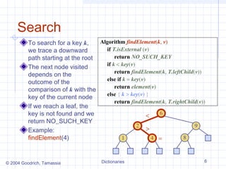
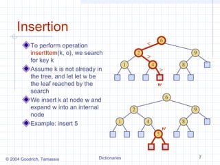
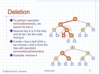
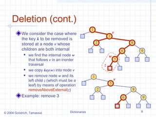
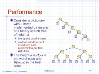
The document describes different data structures that can be used to implement dictionaries, including log files, lookup tables, binary search trees, and hash tables. It explains the basic operations for each structure, such as search, insertion, and deletion times. Binary search trees provide efficient search times of O(log n) on average but can degrade to O(n) in the worst case. Hash tables provide expected constant time for search, insertion, and deletion if collisions are handled well.

1. Dictionaries
< 6
2 9
>
1 4 = 8
© 2004 Goodrich, Tamassia Dictionaries 1

2. Dictionary ADT
The dictionary ADT models a Dictionary ADT methods:
searchable collection of key-  findElement(k): if the
element items dictionary has an item with
The main operations of a key k, returns its element,
dictionary are searching, else, returns the special
element NO_SUCH_KEY
inserting, and deleting items  insertItem(k, o): inserts item
Multiple items with the same key (k, o) into the dictionary
are allowed  removeElement(k): if the
Applications: dictionary has an item with
 address book key k, removes it from the
 credit card authorization dictionary and returns its
element, else returns the
 mapping host names (e.g., special element
cs16.net) to internet addresses NO_SUCH_KEY
(e.g., 128.148.34.101)  size(), isEmpty()
 keys(), Elements()
© 2004 Goodrich, Tamassia Dictionaries 2

3. Log File
A log file is a dictionary implemented by means of an unsorted
sequence
 We store the items of the dictionary in a sequence (based on a
doubly-linked lists or a circular array), in arbitrary order
Performance:
 insertItem takes O(1) time since we can insert the new item at the
beginning or at the end of the sequence
 findElement and removeElement take O(n) time since in the worst
case (the item is not found) we traverse the entire sequence to look
for an item with the given key
The log file is effective only for dictionaries of small size or for
dictionaries on which insertions are the most common
operations, while searches and removals are rarely performed
(e.g., historical record of logins to a workstation)
© 2004 Goodrich, Tamassia Dictionaries 3

4. Lookup Table
A lookup table is a dictionary implemented by means of a sorted
sequence
 We store the items of the dictionary in an array-based sequence,
sorted by key
 We use an external comparator for the keys
Performance:
 findElement takes O(log n) time, using binary search
 insertItem takes O(n) time since in the worst case we have to shift
n/2 items to make room for the new item
 removeElement take O(n) time since in the worst case we have to
shift n/2 items to compact the items after the removal
The lookup table is effective only for dictionaries of small size or
for dictionaries on which searches are the most common
operations, while insertions and removals are rarely performed
(e.g., credit card authorizations)
© 2004 Goodrich, Tamassia Dictionaries 4

5. Binary Search Tree
A binary search tree is An inorder traversal of a
a binary tree storing binary search trees
keys (or key-element visits the keys in
pairs) at its internal increasing order
nodes and satisfying
the following property:
 Let u, v, and w be three 6
nodes such that u is in
2 9
the left subtree of v and w
is in the right subtree of 1 4 8
v. We have
key(u) ≤ key(v) ≤ key(w)
External nodes do not
store items
© 2004 Goodrich, Tamassia Dictionaries 5

6. Search
To search for a key k, Algorithm findElement(k, v)
we trace a downward if T.isExternal (v)
path starting at the root return NO_SUCH_KEY
if k < key(v)
The next node visited
return findElement(k, T.leftChild(v))
depends on the
else if k = key(v)
outcome of the
return element(v)
comparison of k with the
else { k > key(v) }
key of the current node
return findElement(k, T.rightChild(v))
If we reach a leaf, the
key is not found and we < 6
return NO_SUCH_KEY
2 9
Example: >
findElement(4) 1 4 = 8
© 2004 Goodrich, Tamassia Dictionaries 6

7. Insertion
6
To perform operation <
insertItem(k, o), we search 2 9
>
for key k
1 4 8
Assume k is not already in >
the tree, and let let w be
the leaf reached by the w
search
6
We insert k at node w and
expand w into an internal 2 9
node
Example: insert 5 1 4 8
w
5
© 2004 Goodrich, Tamassia Dictionaries 7

8. Deletion
6
To perform operation <
removeElement(k), we 2 9
search for key k >
1 4 v 8
Assume key k is in the tree,
w
and let let v be the node 5
storing k
If node v has a leaf child w,
we remove v and w from the
tree with operation 6
removeAboveExternal(w)
2 9
Example: remove 4
1 5 8
© 2004 Goodrich, Tamassia Dictionaries 8

9. Deletion (cont.)
1
We consider the case where v
3
the key k to be removed is
stored at a node v whose 2 8
children are both internal 6 9
 we find the internal node w w
that follows v in an inorder 5
traversal z
 we copy key(w) into node v
 we remove node w and its 1
left child z (which must be a v
leaf) by means of operation 5
removeAboveExternal(z) 2 8
Example: remove 3 6 9
© 2004 Goodrich, Tamassia Dictionaries 9

10. Performance
Consider a dictionary
with n items
implemented by means
of a binary search tree
of height h
 the space used is O(n)
 methods findElement ,
insertItem and
removeElement take
O(h) time
The height h is O(n) in
the worst case and
O(log n) in the best
case
© 2004 Goodrich, Tamassia Dictionaries 10

11. Ordered Dictionaries
Keys are assumed to come from a total
order.
New operations:
 first(): first entry in the dictionary ordering
 last(): last entry in the dictionary ordering
 successors(k): iterator of entries with keys
greater than or equal to k; increasing order
 predecessors(k): iterator of entries with keys
less than or equal to k; decreasing order
© 2004 Goodrich, Tamassia Bucket-Sort and Radix-Sort 11

12. Hash Tables
0 ∅
1 025-612-0001
2 981-101-0002
3 ∅
4 451-229-0004
© 2004 Goodrich, Tamassia Hash Tables 12

13. Recall the Map ADT
Map ADT methods:
 get(k): if the map M has an entry with key k, return
its assoiciated value; else, return null
 put(k, v): insert entry (k, v) into the map M; if key k
is not already in M, then return null; else, return
old value associated with k
 remove(k): if the map M has an entry with key k,
remove it from M and return its associated value;
else, return null
 size(), isEmpty()
 keys(): return an iterator of the keys in M
 values(): return an iterator of the values in M
© 2004 Goodrich, Tamassia Hash Tables 13

14. Hash Functions and
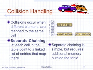
Hash Tables
A hash function h maps keys of a given type to integers
in a fixed interval [0, N − 1]
Example:
h(x) = x mod N
is a hash function for integer keys
The integer h(x) is called the hash value of key x
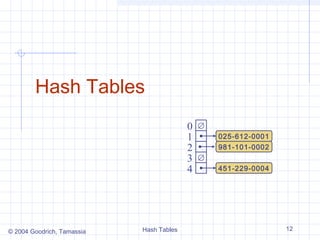
A hash table for a given key type consists of
 Hash function h
 Array (called table) of size N
When implementing a map with a hash table, the goal
is to store item (k, o) at index i = h(k)
© 2004 Goodrich, Tamassia Hash Tables 14

15. Example
We design a hash table for 0 ∅
a map storing entries as 1 025-612-0001
(SSN, Name), where SSN 2 981-101-0002
3 ∅
(social security number) is a 4 451-229-0004
nine-digit positive integer
…
Our hash table uses an
array of size N = 10,000 and 9997 ∅
9998 200-751-9998
the hash function 9999 ∅
h(x) = last four digits of x
© 2004 Goodrich, Tamassia Hash Tables 15

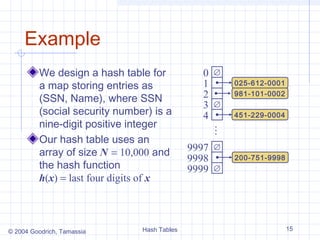
16. Hash Functions
A hash function is The hash code is
usually specified as the applied first, and the
compression function
composition of two
is applied next on the
functions: result, i.e.,
Hash code: h(x) = h2(h1(x))
h1: keys → integers The goal of the hash
function is to
Compression function:
“disperse” the keys in
h2: integers → [0, N − 1] an apparently random
way
© 2004 Goodrich, Tamassia Hash Tables 16

17. Hash Codes
Memory address: Component sum:
 We reinterpret the memory  We partition the bits of
address of the key object as the key into components
an integer (default hash code
of fixed length (e.g., 16 or
of all Java objects)
32 bits) and we sum the
 Good in general, except for components (ignoring
numeric and string keys
overflows)
Integer cast:  Suitable for numeric keys
 We reinterpret the bits of the of fixed length greater
key as an integer than or equal to the
 Suitable for keys of length number of bits of the
less than or equal to the integer type (e.g., long
number of bits of the integer
and double in Java)
type (e.g., byte, short, int and
float in Java)
© 2004 Goodrich, Tamassia Hash Tables 17

18. Hash Codes (cont.)
Polynomial accumulation: Polynomial p(z) can be
 We partition the bits of the evaluated in O(n) time
key into a sequence of
components of fixed length
using Horner’s rule:
(e.g., 8, 16 or 32 bits)  The following
a0 a1 … an−1 polynomials are
 We evaluate the polynomial successively computed,
p(z) = a0 + a1 z + a2 z2 + … each from the previous
… + an−1zn−1 one in O(1) time
at a fixed value z, ignoring p0(z) = an−1
overflows pi (z) = an−i−1 + zpi−1(z)
 Especially suitable for strings (i = 1, 2, …, n −1)
(e.g., the choice z = 33 gives
at most 6 collisions on a set of We have p(z) = pn−1(z)
50,000 English words)
© 2004 Goodrich, Tamassia Hash Tables 18

19. Compression Functions
Division: Multiply, Add and
 h2 (y) = y mod N Divide (MAD):
 The size N of the  h2 (y) = (ay + b) mod N
hash table is usually  a and b are
chosen to be a prime nonnegative integers
 The reason has to do such that
with number theory a mod N ≠ 0
and is beyond the  Otherwise, every
scope of this course integer would map to
the same value b
© 2004 Goodrich, Tamassia Hash Tables 19

20. Example (ideal) hash function
0 kiwi
Suppose our hash function 1
gave us the following values: 2 banana
hashCode("apple") = 5 3 watermelon
hashCode("watermelon") = 3
hashCode("grapes") = 8 4
hashCode("cantaloupe") = 7
hashCode("kiwi") = 0
5 apple
hashCode("strawberry") = 9 6 mango
hashCode("mango") = 6
hashCode("banana") = 2 7 cantaloupe
8 grapes
9 strawberry
© 2004 Goodrich, Tamassia

21. Collisions
When two values hash to the same array
location, this is called a collision
Collisions are normally treated as “first
come, first served”—the first value that
hashes to the location gets it
We have to find something to do with the
second and subsequent values that hash
to this same location
© 2004 Goodrich, Tamassia

22. Collision Handling
Collisions occur when 0 ∅
1 025-612-0001
different elements are 2 ∅
mapped to the same 3 ∅
cell 4 451-229-0004 981-101-0004
Separate Chaining:
let each cell in the Separate chaining is
table point to a linked simple, but requires
list of entries that map additional memory
there outside the table
© 2004 Goodrich, Tamassia Hash Tables 22

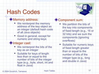
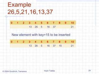
23. Linear probing
A simple open addressing collision handling strategy
is called linear probing. In this if we try to insert an
item (k,e) into a bucket A[i] that is already occupied ,
where i=h(k), then we try next at A[(i+1)mod N]. If
A[(i+1)mod N] is occupied then we try at A[(i+2)mod
N] and so on, until we find the empty bucket in A that
can accept the new item.
© 2004 Goodrich, Tamassia Hash Tables 23

24. Example
26,5,21,16,13,37
0 1 2 3 4 5 6 7 8 9 10
13 26 5 16 37 21
New element with key=15 to be inserted
0 1 2 3 4 5 6 7 8 9 10
13 26 5 16 37 15 21
© 2004 Goodrich, Tamassia Hash Tables 24