1. Nick Heydman
PHY 432L
Experiment 3
Detector Efficiency
1.Effective Distance of the Detector
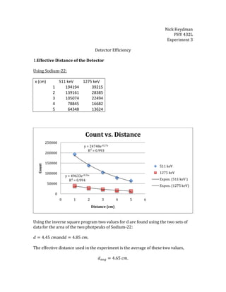
Using Sodium-22:
x (cm) 511 keV 1275 keV
1 194194 39215
2 139161 28385
3 105074 22494
4 78845 16682
5 64348 13624
Using the inverse square program two values for d are found using the two sets of
data for the area of the two photpeaks of Sodium-22:
and .
The effective distance used in the experiment is the average of these two values,
y = 24748e-0.27x
R² = 0.993
y = 49633e-0.26x
R² = 0.994
0
50000
100000
150000
200000
250000
0 1 2 3 4 5 6
Count
Distance (cm)
Count vs. Distance
511 keV
1275 keV
Expon. (511 keV )
Expon. (1275 keV)
2. 2. Measuring Efficiency
Calculating the Geometry Factor
,
.
x (cm) G
1 0.070483202
2 0.050879077
3 0.038446751
4 0.030071168
5 0.024161722
As the distance is increased away from the detector, the Geometric Factor begins to
decrease. This represents a reduction in gammas detected by the detector.
Calculating the Activity
A' (microCi) Age (yrs) Half-Life (yrs) Decay Constant Lifetime
Na-22 7.97 6.5 2.62 0.264559993 3.779861007
Cs-137 1.12 27.5 30 0.023104906 43.28085123
Co-60 12.27 23.7 5.2714 0.131492048 7.605022639
Bi-207 1.038 5.5 31.55 0.0219698 45.51702854
3. All measurements were taken one centimeter away from the detector.
Sodium-22
Cesium-137
Cobalt-60
Bismuth-207
3. Efficiency as a Function of Energy
4. From the calibration graph the energy of the gammas from the Bi-207 can be found.
To find the efficiency of a 1460 keV gamma a log-log plot of the negative log of the
efficiency vs. the log of the energy can be used.
y = -0.0004x + 0.6748
R² = 0.98718
0
0.1
0.2
0.3
0.4
0.5
0.6
0 500 1000 1500
Efficiency
Energy (keV)
Efficiency vs. Energy
Efficiency vs. Energy
Linear (Efficiency vs.
Energy)
Isotope
Count
(1/min)
Activity
(decays/min) Yield G Efficiency Energy (keV)
Na-22 194104 3171442.973 1.8 0.0705 0.48229855 511
Cs-137 34283 1316820.234 0.85 0.0705 0.434454485 662
Co-60 17290 1208244.289 1 0.0705 0.202979008 1173.237
Na-22 43415 3171442.973 1 0.0705 0.194175209 1275
Co-60 15626 1208244.289 1 0.0705 0.183444186 1332.501
Bi-207 63196 2041663 0.977 0.0705 0.449388393 562.7790168
Bi-207 26787 2041663 0.745 0.0705 0.249801263 1061.746843
5. A power trendline fit is used.
negative log efficiency log energy
0.32097492 2.7084209
0.366346592 2.820857989
0.696839751 3.069385751
0.716097095 3.105510185
0.740786925 3.124667544
4. Activity of the Salt Sample
y = 0.0006x6.2546
R² = 0.98559
0
0.1
0.2
0.3
0.4
0.5
0.6
0.7
0.8
2.6 2.7 2.8 2.9 3 3.1 3.2
-log(efficiency)
log(E)
Log-Log Plot
Log-Log Plot
Power (Log-Log Plot)
6. Four-Hour Background
Two-Hour Data
Detection
Activity
Error
The Geometric Factor contains error as well as the instrumentation itself.
Because the total error in the efficiency calibration can total to 10% - 30% and the
Effective Distance, d was averaged, the Geometric Factor error should average 20%.
The activity with the geometric error is
7. The detector is calibrated at 5% error.
Therefore,
5. Alternate Method to Calculate Activity
This value is not in the range calculated above. The alternate method produces a
value about twice that of the calculated activity above. The equation derived might
be incorrect or off by a factor of two.
6. Photoelectric Effect or Compton Scattering
8. For a 1000 keV gamma ray, the more probable effect would be Compton scattering.
The photoelectric effect is more common at lower energies, at or around 50 eV. The
photoelectric effect occurs when an electron is ejected from the nucleus of an atom
because of the transfer of energy from a photon. With sufficient energy not only will
the electron be ionized, but a lower energy photon will be emitted from the electron,
causing the electron to scatter.
At 1000 keV there is a large amount of energy for the electron to not only ionize, but
also emit photons with relatively large energy.
- Compton Scattering