This document provides an overview and preface for the book "Detection, Estimation, and Modulation Theory, Part I" by Harry L. Van Trees. The book covers detection and estimation theory, which combines classical statistical inference techniques with modeling of communication, radar, and other data processing systems using random processes. Part I focuses on detection, estimation, and linear modulation theory. It has been widely used as a textbook since its publication in 1968. The author developed the material from his teaching notes to provide graduate students with a unified presentation of detection, estimation, and modulation theory.

1. Part I

2. Detection, Estimation, and Modulation Theory, Part I:
Detection, Estimation, and Linear Modulation Theory. Harry L. Van Trees
Copyright© 2001 John Wiley & Sons, Inc.
ISBNs: 0-471-09517-6 (Paperback); 0-471-22108-2 (Electronic)
Detection, Estimation, and Modulation Theory

3. Detection, Estimation,
and Modulation Theory
Part I. Detection, Estimation,
and Linear Modulation Theory
HARRY L. VAN TREES
George Mason University
A Wiley-Interscience Publication
JOHN WILEY & SONS, INC.
New York • Chichester • Weinheim • Brisbane • Singapore • Toronto

4. This text is printed on acid-free paper. @)
Copyright© 2001 by John Wiley & Sons, Inc. All rights reserved.
Published simultaneously in Canada.
No part ofthis publication may be reproduced, stored in a retrieval system or transmitted in any
form or by any means, electronic, mechanical, photocopying, recording, scanning or otherwise,
except as permitted under Section I07 or I08 ofthe 1976 United States Copyright Act, without
either the prior written permission ofthe Publisher, or authorization through payment ofthe
appropriate per-copy fee to the Copyright Clearance Center, 222 Rosewood Drive, Danvers, MA
01923, (978) 750-8400, fax (978) 750-4744. Requests to the Publisher for permission should be
addressed to the Permissions Department, John Wiley & Sons, Inc., 605 Third Avenue, New York,
NY 10158-0012, (212) 850-6011, fax (212) 850-6008, E-Mail: PERMREQ@ WILEY.COM.
For ordering and customer service, call 1-800-CALL-WILEY.
Library ofCongress Cataloging in Publication Data is available.
ISBN 0-471-22108-2
This title is also available in print as ISBN 0-471-09517-6.
Printed in the United States of America
10 9 8 7 6 5 4 3 2 I

5. To Diane
and Stephen, Mark, Kathleen, Patricia,
Eileen, Harry, and Julia
and the next generation-
Brittany, Erin, Thomas, Elizabeth, Emily,
Dillon, Bryan, Julia, Robert, Margaret,
Peter, Emma, Sarah, Harry, Rebecca,
and Molly

7. Prefacefor Paperback Edition
In 1968, Part I of Detection, Estimation, and Modulation Theory [VT68) was pub-
lished. It turned out to be a reasonably successful book that has been widely used by
several generations of engineers. There were thirty printings, but the last printing
was in 1996. Volumes II and III ([VT71a], [VT71b]) were published in 1971 and fo-
cused on specific application areas such as analog modulation, Gaussian signals
and noise, and the radar-sonar problem. Volume II had a short life span due to the
shift from analog modulation to digital modulation. Volume III is still widely used
as a reference and as a supplementary text. In a moment ofyouthful optimism, I in-
dicated in the the Preface to Volume III and in Chapter III-14 that a short mono-
graph on optimum array processing would be published in 1971. The bibliography
lists it as a reference, Optimum Array Processing, Wiley, 1971, which has been sub-
sequently cited by several authors. After a 30-year delay, Optimum Array Process-
ing, Part IV ofDetection, Estimation, and Modulation Theory will be published this
year.
A few comments on my career may help explain the long delay. In 1972, MIT
loaned me to the Defense Communication Agency in Washington, D.C. where I
spent three years as the Chief Scientist and the Associate Director ofTechnology. At
the end of the tour, I decided, for personal reasons, to stay in the Washington, D.C.
area. I spent three years as an Assistant Vice-President at COMSAT where my
group did the advanced planning for the INTELSAT satellites. In 1978, I became
the Chief Scientist ofthe United States Air Force. In 1979, Dr. Gerald Dinneen, the
former Director of Lincoln Laboratories, was serving as Assistant Secretary of De-
fense for C31. He asked me to become his Principal Deputy and I spent two years in
that position. In 1981, I joined M/A-COM Linkabit. Linkabit is the company that Ir-
win Jacobs and Andrew Viterbi had started in 1969 and sold to MIA-COM in 1979.
I started an Eastern operation which grew to about 200 people in three years. After
Irwin and Andy left MIA-COM and started Qualcomm, I was responsible for the
government operations in San Diego as well as Washington, D.C. In 1988, MIA-
COM sold the division. At that point I decided to return to the academic world.
I joined George Mason University in September of 1988. One of my priorities
was to finish the book on optimum array processing. However, I found that I needed
to build up a research center in order to attract young research-oriented faculty and
vii

8. viii Prefacefor Paperback Edition
doctoral students. The process took about six years. The Center for Excellence in
Command, Control, Communications, and Intelligence has been very successful
and has generated over $300 million in research funding during its existence. Dur-
ing this growth period, I spent some time on array processing but a concentrated ef-
fort was not possible. In 1995, I started a serious effort to write the Array Process-
ing book.
Throughout the Optimum Array Processing text there are references to Parts I
and III ofDetection, Estimation, and Modulation Theory. The referenced material is
available in several other books, but I am most familiar with my own work. Wiley
agreed to publish Part I and III in paperback so the material will be readily avail-
able. In addition to providing background for Part IV, Part I is still useful as a text
for a graduate course in Detection and Estimation Theory. Part III is suitable for a
second level graduate course dealing with more specialized topics.
In the 30-year period, there has been a dramatic change in the signal processing
area. Advances in computational capability have allowed the implementation of
complex algorithms that were only of theoretical interest in the past. In many appli-
cations, algorithms can be implemented that reach the theoretical bounds.
The advances in computational capability have also changed how the material is
taught. In Parts I and III, there is an emphasis on compact analytical solutions to
problems. In Part IV, there is a much greater emphasis on efficient iterative solu-
tions and simulations. All ofthe material in parts I and III is still relevant. The books
use continuous time processes but the transition to discrete time processes is
straightforward. Integrals that were difficult to do analytically can be done easily in
Matlab®. The various detection and estimation algorithms can be simulated and
their performance compared to the theoretical bounds. We still use most ofthe prob-
lems in the text but supplement them with problems that require Matlab® solutions.
We hope that a new generation of students and readers find these reprinted edi-
tions to be useful.
Fairfax, Virginia
June 2001
HARRY L. VAN TREES

9. Preface
The area ofdetection and estimation theory that we shall study in this book
represents a combination of the classical techniques of statistical inference
and the random process characterization of communication, radar, sonar,
and other modern data processing systems. The two major areas of statis-
tical inference are decision theory and estimation theory. In the first case
we observe an output that has a random character and decide which oftwo
possible causes produced it. This type ofproblem was studied in the middle
of the eighteenth century by Thomas Bayes [1]. In the estimation theory
case the output is related to the value of some parameter of interest, and
we try to estimate the value of this parameter. Work in this area was
published by Legendre [2] and Gauss [3] in the early nineteenth century.
Significant contributions to the classical theory that we use as background
were developed by Fisher [4] and Neyman and Pearson [5] more than
30 years ago. In 1941 and 1942 Kolmogoroff [6] and Wiener [7] applied
statistical techniques to the solution of the optimum linear filtering
problem. Since that time the application of statistical techniques to the
synthesis and analysis of all types of systems has grown rapidly. The
application of these techniques and the resulting implications are the
subject of this book.
This book and the subsequent volume, Detection, Estimation, and
Modulation Theory, Part II, are based on notes prepared for a course
entitled "Detection, Estimation, and Modulation Theory," which is taught
as a second-level graduate course at M.I.T. My original interest in the
material grew out ofmy research activities in the area ofanalog modulation
theory. A preliminary version of the material that deals with modulation
theory was used as a text for a summer course presented at M.I.T. in 1964.
It turned out that our viewpoint on modulation theory could best be
understood by an audience with a clear understanding ofmodern detection
and estimation theory. At that time there was no suitable text available to
cover the material of interest and emphasize the points that I felt were
ix

10. x Preface
important, so I started writing notes. It was clear that in order to present
the material to graduate students in a reasonable amount of time it would
be necessary to develop a unified presentation ofthe three topics: detection,
estimation, and modulation theory, and exploit the fundamental ideas that
connected them. As the development proceeded, it grew in size until the
material that was originally intended to be background for modulation
theory occupies the entire contents of this book. The original material on
modulation theory starts at the beginning ofthe second book. Collectively,
the two books provide a unified coverage of the three topics and their
application to many important physical problems.
For the last three years I have presented successively revised versions of
the material in my course. The audience consists typically of 40 to 50
students who have completed a graduate course in random processes which
covered most of the material in Davenport and Root [8]. In general, they
have a good understanding ofrandom process theory and a fair amount of
practice with the routine manipulation required to solve problems. In
addition, many ofthem are interested in doing research in this general area
or closely related areas. This interest provides a great deal of motivation
which I exploit by requiring them to develop many of the important ideas
as problems. It is for this audience that the book is primarily intended. The
appendix contains a detailed outline of the course.
On the other hand, many practicing engineers deal with systems that
have been or should have been designed and analyzed with the techniques
developed in this book. I have attempted to make the book useful to them.
An earlier version was used successfully as a text for an in-plant course for
graduate engineers.
From the standpoint of specific background little advanced material is
required. A knowledge of elementary probability theory and second
moment characterization ofrandom processes is assumed. Some familiarity
with matrix theory and linear algebra is helpful but certainly not necessary.
The level ofmathematical rigor is low, although in most sections the results
could be rigorously proved by simply being more careful in our derivations.
We have adopted this approach in order not to obscure the important
ideas with a lot of detail and to make the material readable for the kind of
engineering audience that will find it useful. Fortunately, in almost all
cases we can verify that our answers are intuitively logical. It is worthwhile
to observe that this ability to check our answers intuitively would be
necessary even if our derivations were rigorous, because our ultimate
objective is to obtain an answer that corresponds to some physical system
of interest. It is easy to find physical problems in which a plausible mathe-
matical model and correct mathematics lead to an unrealistic answer for the
original problem.

11. Preface xi
We have several idiosyncrasies that it might be appropriate to mention.
In general, we look at a problem in a fair amount ofdetail. Many times we
look at the same problem in several different ways in order to gain a better
understanding ofthe meaning ofthe result. Teaching students a number of
ways of doing things helps them to be more flexible in their approach to
new problems. A second feature is the necessity for the reader to solve
problems to understand the material fully. Throughout the course and the
book we emphasize the development ofan ability to work problems. At the
end ofeach chapter are problems that range from routine manipulations to
significant extensions of the material in the text. In many cases they are
equivalent to journal articles currently being published. Only by working a
fair number of them is it possible to appreciate the significance and
generality of the results. Solutions for an individual problem will be
supplied on request, and a book containing solutions to about one third
of the problems is available to faculty members teaching the course. We
are continually generating new problems in conjunction with the course
and will send them to anyone who is using the book as a course text. A
third issue is the abundance of block diagrams, outlines, and pictures. The
diagrams are included because most engineers (including myself) are more
at home with these items than with the corresponding equations.
One problem always encountered is the amount of notation needed to
cover the large range of subjects. We have tried to choose the notation in a
logical manner and to make it mnemonic. All the notation is summarized
in the glossary at the end of the book. We have tried to make our list of
references as complete as possible and to acknowledge any ideas due to
other people.
A number of people have contributed in many ways and it is a pleasure
to acknowledge them. Professors W. B. Davenport and W. M. Siebert have
provided continual encouragement and technical comments on the various
chapters. Professors Estil Hoversten and Donald Snyder of the M.I.T.
faculty and Lewis Collins, Arthur Baggeroer, and Michael Austin, three
of my doctoral students, have carefully read and criticized the various
chapters. Their suggestions have improved the manuscript appreciably. In
addition, Baggeroer and Collins contributed a number of the problems in
the various chapters and Baggeroer didtheprogrammingnecessaryfor many
of the graphical results. Lt. David Wright read and criticized Chapter 2.
L.A. Frasco and H. D. Goldfein, two of my teaching assistants, worked
all ofthe problems in the book. Dr. Howard Yudkin ofLincoln Laboratory
read the entire manuscript and offered a number of important criticisms.
In addition, various graduate students taking the course have made
suggestions which have been incorporated. Most of the final draft was
typed by Miss Aina Sils. Her patience with the innumerable changes is

12. xii Preface
sincerely appreciated. Several other secretaries, including Mrs. Jarmila
Hrbek, Mrs. Joan Bauer, and Miss Camille Tortorici, typed sections of the
various drafts.
As pointed out earlier, the books are an outgrowth of my research
interests. This research is a continuing effort, and I shall be glad to send our
current work to people working in this area on a regular reciprocal basis.
My early work in modulation theory was supported by Lincoln Laboratory
as a summer employee and consultant in groups directed by Dr. Herbert
Sherman and Dr. Barney Reiffen. My research at M.I.T. was partly
supported by the Joint Services and the National Aeronautics and Space
Administration under the auspices of the Research Laboratory of Elec-
tronics. This support is gratefully acknowledged.
Cambridge, Massachusetts
October, 1967.
REFERENCES
Harry L. Van Trees
[1] Thomas Bayes, "An Essay Towards Solving a Problem in the Doctrine of
Chances," Phil. Trans, 53, 370-418 (1764).
[2] A. M. Legendre, Nouvelles Methodes pour La Determination ces Orbites des
Cometes, Paris, 1806.
[3] K. F. Gauss, Theory of Motion of the Heavenly Bodies Moving About the Sun in
Conic Sections, reprinted by Dover, New York, 1963.
[4] R. A. Fisher, "Theory of Statistical Estimation," Proc. Cambridge Philos. Soc.,
11, 700 (1925).
[5] J. Neyman and E. S. Pearson, "On the Problem of the Most Efficient Tests of
Statistical Hypotheses," Phil. Trans. Roy. Soc. London, A 131, 289, (1933).
[6] A. Kolmogoroff, "Interpolation and Extrapolation von Stationiiren Zufiilligen
Folgen," Bull. Acad. Sci. USSR, Ser. Math. 5, 1941.
[7] N. Wiener, Extrapolation, Interpolation, and Smoothing ofStationary Time Series,
Tech. Press of M.I.T. and Wiley, New York, 1949 (originally published as a
classified report in 1942).
[8] W. B. Davenport and W. L. Root, Random Signals and Noise, McGraw-Hill,
New York, 1958.

13. Contents
1 Introduction
2
1.1 Topical Outline
1.2 Possible Approaches
1.3 Organization
Classical Detection and Estimation Theory
2.1 Introduction
2.2 Simple Binary Hypothesis Tests
Decision Criteria. Performance: Receiver Operating Charac-
teristic.
2.3 M Hypotheses
2.4 Estimation Theory
Random Parameters: Bayes Estimation. Real (Nonrandom)
Parameter Estimation. Multiple Parameter Estimation. Sum-
mary of Estimation Theory.
2.5 Composite Hypotheses
2.6 The General Gaussian Problem
Equal Covariance Matrices. Equal Mean Vectors. Summary.
2.7 Performance Bounds and Approximations
2.8 Summary
2.9 Problems
References
1
1
12
15
19
19
23
46
52
86
96
116
133
133
163
xiii

14. xiv Contents
3 Representations of Random Processes 166
3.1 Introduction 166
3.2 Deterministic Functions: Orthogonal Representations 169
3.3 Random Process Characterization 174
Random Processes: Conventional Characterizations. Series
Representation of Sample Functions of Random Processes.
Gaussian Processes.
3.4 Homogeneous Integral Equations and Eigenfunctions 186
Rational Spectra. Bandlimited Spectra. Nonstationary
Processes. White Noise Processes. The Optimum Linear
Filter. Properties of Eigenfunctions and Eigenvalues.
3.5 Periodic Processes
3.6 Infinite Time Interval: Spectral Decomposition
Spectral Decomposition. An Application of Spectral Decom-
position: MAP Estimation of a Gaussian Process.
209
212
3.7 Vector Random Processes 220
3.8 Summary
3.9 Problems
References
4 Detection of Signals-Estimation of Signal
224
226
237
Parameters 239
4.1 Introduction 239
Models. Format.
4.2 Detection and Estimation in White Gaussian Noise 246
Detection of Signals in Additive White Gaussian Noise. Linear
Estimation. Nonlinear Estimation. Summary: Known Signals
in White Gaussian Noise.
4.3 Detection and Estimation in Nonwhite Gaussian Noise 287
"Whitening" Approach. A Direct Derivation Using the
Karhunen-Loeve Expansion. A Direct Derivation with a
Sufficient Statistic. Detection Performance. Estimation.
Solution Techniques for Integral Equations. Sensitivity.
Known Linear Channels.

15. Contents XV
4.4 Signals with Unwanted Parameters: The Composite Hypo-
thesis Problem 333
Random Phase Angles. Random Amplitude and Phase.
4.5 Multiple Channels 366
Formulation. Application.
4.6 Multiple Parameter Estimation 370
Additive White Gaussian Noise Channel. Extensions.
4.7 Summary and Omissions 374
Summary. Topics Omitted.
4.8 Problems 377
References 418
5 Estimation of Continuous Waveforms 423
5.1 Introduction 423
5.2 Derivation of Estimator Equations 426
No-Memory Modulation Systems. Modulation Systems with
Memory.
5.3 A Lower Bound on the Mean-Square Estimation Error 437
5.4 Multidimensional Waveform Estimation 446
Examples of Multidimensional Problems. Problem Formula-
tion. Derivation of Estimator Equations. Lower Bound on
the Error Matrix. Colored Noise Estimation.
5.5 Nonrandom Waveform Estimation 456
5.6 Summary 459
5.7 Problems 460
References 465
6 Linear Estimation 467
6.1 Properties of Optimum Processors 468
6.2 Realizable Linear Filters: Stationary Processes, Infinite
Past: Wiener Filters 481
Solution of Wiener-Hopf Equation. Errors in Optimum
Systems. Unrealizable Filters. Closed-FormError Expressions.
Optimum Feedback Systems. Comments.

16. xvi Contents
6.3 Kalman-Bucy Filters 515
Differential Equation Representation of Linear Systems and
Random Process Generation. Derivation of Estimator Equa-
tions. Applications. Generalizations.
6.4 Linear Modulation: Communications Context 575
DSB-AM: Realizable Demodulation. DSB-AM: Demodula-
tion with Delay. Amplitude Modulation: Generalized Carriers.
Amplitude Modulation: Single-Sideband Suppressed-Carrier.
6.5 The Fundamental Role of the Optimum Linear Filter 584
6.6 Comments 585
6.7 Problems 586
References 619
7 Discussion 623
7.1 Summary 623
7.2 Preview of Part II 625
7.3 Unexplored Issues 627
References 629
Appendix: A Typical Course Outline 635
Glossary 671
Author Index 683
Subject Index 687

17. 1
Detection, Estimation, and Modulation Theory, Part I:
Detection, Estimation, and Linear Modulation Theory. Harry L. Van Trees
Copyright © 2001 John Wiley & Sons, Inc.
ISBNs: 0-471-09517-6 (Paperback); 0-471-22108-2 (Electronic)
Introduction
In these two books, we shall study three areas of statistical theory, which
we have labeled detection theory, estimation theory, and modulation
theory. The goal is to develop these theories in a common mathematical
framework and to demonstrate how they can be used to solve a wealth of
practical problems in many diverse physical situations.
In this chapter we present three outlines of the material. The first is a
topical outline in which we develop a qualitative understanding ofthe three
areas by examining some typical problems of interest. The second is a
logical outline in which we explore the various methods of attacking the
problems. The third is a chronological outline in which we explain the
structure of the books.
1.1 TOPICAL OUTLINE
An easy way to explain what is meant by detection theory is to examine
several physical situations that lead to detection theory problems.
A simple digital communication system is shown in Fig. 1.1. The source
puts out a binary digit every T seconds. Our object is to transmit this
sequence of digits to some other location. The channel available for trans-
mitting the sequence depends on the particular situation. Typically, it
could be a telephone line, a radio link, or an acoustical channel. For
r(t)
Fig. 1.1 Digital communication system.
1

18. 2 1.1 Topical Outline
purposes ofillustration, we shall consider a radio link. In order to transmit
the information, we must put it into a form suitable for propagating over
the channel. A straightforward method would be to build a device that
generates a sine wave,
(1)
for T seconds if the source generated a "one" in the preceding interval,
and a sine wave of a different frequency,
s0(t) = sin w0 t, (2)
for T seconds if the source generated a "zero" in the preceding interval.
The frequencies are chosen so that the signals s0 (t) and s1(t) will propagate
over the particular radio link of concern. The output of the device is fed
into an antenna and transmitted over the channel. Typical source and
transmitted signal sequences are shown in Fig. 1.2. In the simplest kind of
channel the signal sequence arrives at the receiving antenna attenuated but
essentially undistorted. To process the received signal we pass it through
the antenna and some stages of rf-amplification, in the course of which a
thermal noise n(t) is added to the message sequence. Thus in any T-second
interval we have available a waveform r(t) in which
r(t) = s1(t) + n(t),
if s1(t) was transmitted, and
r(t) = s0(t) + n(t),
0 :s; t :s; T, (3)
(4)
if s0(t) was transmitted. We are now faced with the problem of deciding
which ofthe two possible signals was transmitted. We label the device that
does this a decision device. It is simply a processor that observes r(t) and
guesses whether s1(t) or s0(t) was sent according to some set of rules. This
is equivalent to guessing what the source output was in the preceding
interval. We refer to designing and evaluating the processor as a detection
1 0 0
--------
Source output
sin w1t sin wot sin wot sin w1t
~~~-
Transmitted sequence
Fig. 1.2 Typical sequences.

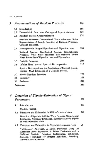
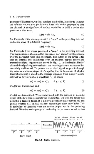
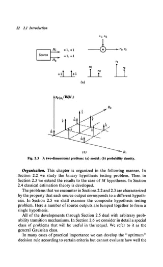
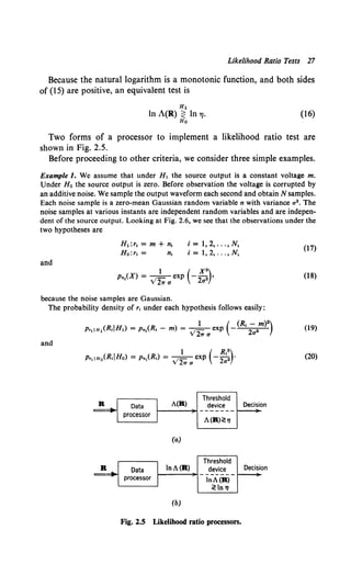
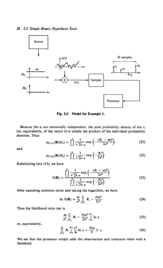
19. Detection Theory 3
If ( r J[ [ J
i7 A~i VVI
I• ~I
sin (Wit + BI) sin (wot + Bo) sin (Wit + Bj)
Fig. 1.3 Sequence with phase shifts.
theory problem. In this particular case the only possible source oferror in
making a decision is the additive noise. If it were not present, the input
would be completely known and we could make decisions without errors.
We denote this type of problem as the known signal in noise problem. It
corresponds to the lowest level (i.e., simplest) of the detection problems of
interest.
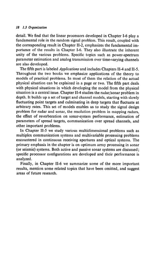
An example of the next level of detection problem is shown in Fig. 1.3.
The oscillators used to generate s1(t) and s0{t) in the preceding example
have a phase drift. Therefore in a particular T-second interval the received
signal corresponding to a "one " is
(5)
and the received signal corresponding to a "zero" is
r(t) = sin (w0 t + 90) + n(t), (6)
where 90 and 91 are unknown constant phase angles. Thus even in the
absence ofnoise the input waveform is not completely known. In a practical
system the receiver may include auxiliary equipment to measure the oscilla-
tor phase. If the phase varies slowly enough, we shall see that essentially
perfect measurement is possible. If this is true, the problem is the same as
above. However, if the measurement is not perfect, we must incorporate
the signal uncertainty in our model.
A corresponding problem arises in the radar and sonar areas. A con-
ventional radar transmits a pulse at some frequency we with a rectangular
envelope:
s1(t) = sin wet, (7)
If a target is present, the pulse is reflected. Even the simplest target will
introduce an attenuation and phase shift in the transmitted signal. Thus
the signal available for processing in the interval of interest is
r(t) = V, sin [we(t - T) + 8,] + n(t),
= n(t),
7' s; t s; 7' + T,
0 s; t < T, -r + T < t < oo, (8)

20. 4 1.1 Topical Outline
if a target is present and
r(t) = n(t), 0 :s; t < oo, (9)
if a target is absent. We see that in the absence of noise the signal still
contains three unknown quantities: Vn the amplitude, ()" the phase, and
r, the round-trip travel time to the target.
These two examples represent the second level of detection problems.
We classify them as signal with unknown parameters in noise problems.
Detection problems of a third level appear in several areas. In a passive
sonar detection system the receiver listens for noise generated by enemy
vessels. The engines, propellers, and other elements in the vessel generate
acoustical signals that travel through the ocean to the hydrophones in the
detection system. This composite signal can best be characterized as a
sample function from a random process. In addition, the hydrophone
generates self-noise and picks up sea noise. Thus a suitable model for the
detection problem might be
r(t) = s0 (t) + n(t) (10)
if the target is present and
r(t) = n(t) (11)
if it is not. In the absence of noise the signal is a sample function from a
random process (indicated by the subscript 0).
In the communications field a large number of systems employ channels
in which randomness is inherent. Typical systems are tropospheric scatter
links, orbiting dipole links, and chaff systems. A common technique is to
transmit one of two signals separated in frequency. (We denote these
frequencies as w1 and w0.) The resulting received signal is
r(t) = s01 (t) + n(t) (12)
if s1(t) was transmitted and
r(t) = S00 (t) + n(t) (13)
if s0(t) was transmitted. Here s01 (t) is a sample function from a random
process centered at w1o and s00 (t) is a sample function from a random
process centered at w0• These examples are characterized by the lack ofany
deterministic signal component. Any decision procedure that we design
will have to be based on the difference in the statistical properties of the
two random processes from which s00 {t) and s01 (t) are obtained. This is
the third level of d~tection problem and is referred to as a random signal
in noise problem.

21. Estimation Theory 5
In our examination of representative examples we have seen that detec-
tion theory problems are characterized by the fact that we must decide
which of several alternatives is true. There were only two alternatives in
the examples cited; therefore we refer to them as binary detection prob-
lems. Later we will encounter problems in which there are M alternatives
available (the M-ary detection problem). Our hierarchy of detection
problems is presented graphically in Fig. 1.4.
There is a parallel set of problems in the estimation theory area. A
simple example is given in Fig. 1.5, in which the source puts out an
analog message a(t) (Fig. 1.5a). To transmit the message we first sample it
every T seconds. Then, every T seconds we transmit a signal that contains
Detection theory
Level 1. Known signals in 1. Synchronous digital communication
noise 2. Pattern recognition problems
Level 2. Signals with unknown 1. Conventional pulsed radar or sonar,
parameters in noise target detection
2. Target classification (orientation of
target unknown)
3. Digital communication systems without
phase reference
4. Digital communication over slowly-
fading channels
Level 3. Random signals in 1. Digital communication over scatter
noise link, orbiting dipole channel, or
chaff link
2. Passive sonar
3. Seismic detection system
4. Radio astronomy (detection of noise
sources)
Fig. 1.4 Detection theory hierarchy.

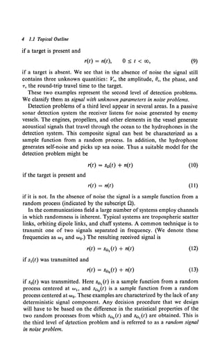
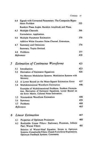
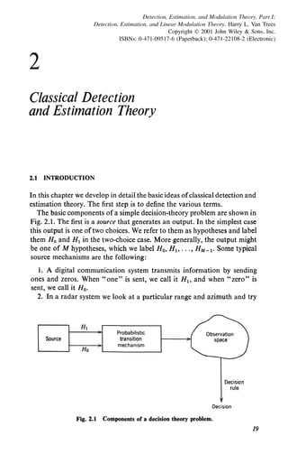
22. 6 1.1 Topical Outline
a(t)
--........ r:
"-...7
a(t)
ITransmitter t-1---------;),..
. . s(t, An)
(a)
(b)
l
Aa
a.(t)
(Frequency changes
I exaggerated)
f f ! AAAAf f
VVVVVWIJV
(c)
A
A
A,
s(t, An)
At
I "
I ~a(t) r
A2
I
J "C/
A3
)I
a.(t) Filter
fi(t)
~
(d)
Fig. 1.5 (a) Sampling an analog source; (b) pulse-amplitude modulation; (c) pulse-
frequency modulation; (d) waveform reconstruction.
a parameter which is uniquely related to the last sample value. In Fig. 1.5b
the signal is a sinusoid whose amplitude depends on the last sample. Thus,
if the sample at time nTis A,., the signal in the interval [nT, (n + l)T] is
nT s t s (n + l)T. (14)
A system of this type is called a pulse amplitude modulation (PAM)
system. In Fig. 1.5c the signal is a sinusoid whose frequency in the interval

23. Estimation Theory 7
differs from the reference frequency we by an amount proportional to the
preceding sample value,
s(t, A,.) = sin (wet + A,.t), nT::;; t ::;; (n + l)T. (15)
A system ofthis type is called a pulse frequency modulation (PFM) system.
Once again there is additive noise. The received waveform, given that A,.
was the sample value, is
r(t) = s(t, A,.) + n(t), nT::;; t ::;; (n + l)T. (16)
During each interval the receiver tries to estimate A,.. We denote these
estimates as A,.. Over a period of time we obtain a sequence of estimates,
as shown in Fig. 1.5d, which is passed into a device whose output is an
estimate of the original message a(t). If a(t) is a band-limited signal, the
device is just an ideal low-pass filter. For other cases it is more involved.
If, however, the parameters in this example were known and the noise
were absent, the received signal would be completely known. We refer
to problems in this category as known signal in noise problems. If we
assume that the mapping from A,. to s(t, A,.) in the transmitter has an
inverse, we see that if the noise were not present we could determine A,.
unambiguously. (Clearly, if we were allowed to design the transmitter, we
should always choose a mapping with an inverse.) The known signal in
noise problem is the first level of the estimation problem hierarchy.
Returning to the area of radar, we consider a somewhat different
problem. We assume that we know a target is present but do not know
its range or velocity. Then the received signal is
r(t) = V, sin [(we + wa)(t - -r) + 8,] + n(t), -r ::;; t ::;; -r + T,
= n(t), 0 ::;; t < -r, -r + T < t < oo,
(17)
where wa denotes a Doppler shift caused by the target's motion. We want
to estimate -rand wa. Now, even if the noise were absent and 1' and wa
were known, the signal would still contain the unknown parameters V,
and 8,. This is a typical second-level estimation problem. As in detection
theory, we refer to problems in this category as signal with unknown
parameters in noise problems.
At the third level the signal component is a random process whose
statistical characteristics contain parameters we want to estimate. The
received signal is of the form
r(t) = sn(t, A) + n(t), (18)
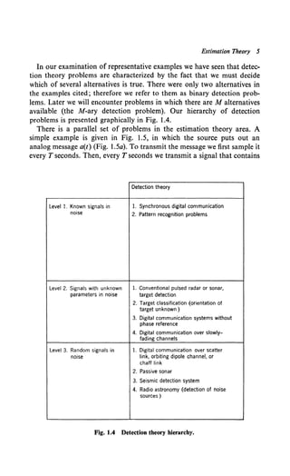
where sn(t, A) is a sample function from a random process. In a simple
case it might be a stationary process with the narrow-band spectrum shown
in Fig. 1.6. The shape of the spectrum is known but the center frequency

24. Spectrum of s0 (t, A)
----~-r~---------------r--------------£_-r~--~r
Center frequency
Fig. 1.6 Spectrum of random signal.
Estimation Theory
Level l. Known signals in noise l. PAM, PFM, and PPM communication systems
with phase synchronization
2. Inaccuracies in inertial systems
(e.g., drift angle measurement)
Level 2. Signals with unknown l. Range, velocity, or angle measurement in
parameters in noise radar/sonar problems
2. Discrete time, continuous amplitude communication
system (with unknown amplitude or phase in
channel)
Level 3. Random signals in noise 1. Power spectrum parameter estimation
2. Range or Doppler spread target parameters
in radar{sonar problem
3. Velocity measurement in radio astronomy
4. Target parameter estimation: passive sonar
5. Ground mapping radars
Fig. 1.7 Estimation theory hierarchy.
8

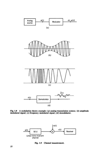
25. Modulation Theory 9
is not. The receiver must observe r(t) and, using the statistical properties
of s0 (t, A) and n(t), estimate the value of A. This particular example could
arise in either radio astronomy or passive sonar. The general class of
problem in which the signal containing the parameters is a sample function
from a random process is referred to as the random signal in noise problem.
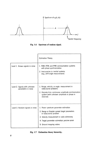
The hierarchy of estimation theory problems is shown in Fig. 1.7.
We note that there appears to be considerable parallelism in the detection
and estimation theory problems. We shall frequently exploit these parallels
to reduce the work, but there is a basic difference that should be em-
phasized. In binary detection the receiver is either "right" or "wrong."
In the estimation of a continuous parameter the receiver will seldom be
exactly right, but it can try to be close most of the time. This difference
will be reflected in the manner in which we judge system performance.
The third area of interest is frequently referred to as modulation theory.
We shall see shortly that this term is too narrow for the actual problems.
Once again a simple example is useful. In Fig. 1.8 we show an analog
message source whose output might typically be music or speech. To
convey the message over the channel, we transform it by using a modula-
tion scheme to get it into a form suitable for propagation. The transmitted
signal is a continuous waveform that depends on a(t) in some deterministic
manner. In Fig. 1.8 it is an amplitude modulated waveform:
s[t, a(t)] = [1 + ma(t)] sin (wet). (19)
(This is conventional double-sideband AM with modulation index m.) In
Fig. l.Sc the transmitted signal is a frequency modulated (FM) waveform:
s[t, a(t)] = sin [wet + f"'a(u) du]. (20)
When noise is added the received signal is
r(t) = s[t, a(t)] + n(t). (21)
Now the receiver must observe r(t) and put out a continuous estimate of
the message a(t), as shown in Fig. 1.8. This particular example is a first-
level modulation problem, for ifn(t) were absent and a(t) were known the
received signal would be completely known. Once again we describe it as
a known signal in noise problem.
Another type of physical situation in which we want to estimate a
continuous function is shown in Fig. 1.9. The channel is a time-invariant
linear system whose impulse response h(T) is unknown. To estimate the
impulse response we transmit a known signal x(t). The received signal is
r(t) = fo''" h(T) x(t - T) dT + n(t). (22)

26. s[t, a(t))
(a)
(c)
~(t)
1" (' (' ,..
VV)
r(t)
ill Demodulator
(d)
Fig. 1.8 A modulation theory example: (a) analog transmission system; (b) amplitude
modulated signal; (c) frequency modulated signal; (d) demodulator.
10
Linear time-invariant
channel
Fig. 1.9 Channel measurement.

27. Modulation Theory 11
The receiver observes r(t) and tries to estimate h(T). This particularexample
could best be described as a continuous estimation problem. Many other
problems of interest in which we shall try to estimate a continuous wave-
form will be encountered. For convenience, we shall use the term modula-
tion theory for this category, even though the term continuous waveform
estimation might be more descriptive.
The other levels of the modulation theory problem follow by direct
analogy. In the amplitude modulation system shown in Fig. 1.8b the
receiver frequently does not know the phase angle of the carrier. In this
case a suitable model is
r(t) = (1 + ma(t)) sin (wet + 8) + n(t), (23)
Modulation Theory (Continuous waveform estimation)
1. Known signals in noise 1. Conventional communication systems
such as AM (DSB-AM, SSB), FM,and
PM with phase synchronization
2. Optimum filter theory
3. Optimum feedback systems
4. Channel measurement
5. Orbital estimation for satellites
6. Signal estimation in seismic and
sonar classification systems
7. Synchronization in digital systems
2. Signals with unknown 1. Conventional communication systems
parameters in noise without phase synchronization
2. Estimation of channel characteristics when
phase of input signal is unknown
3. Random signals in noise 1. Analog communication over
randomly varying channels
2. Estimation of statistics of
time-varying processes
3. Estimation of plant characteristics
Fig. 1.10 Modulation theory hierarchy.

28. 12 1.2 Possible Approaches
where () is an unknown parameter. This is an example of a signal with
unknown parameter problem in the modulation theory area.
A simple example of a third-level problem (random signal in noise) is one
in which we transmit a frequency-modulated signal over a radio link whose
gain and phase characteristics are time-varying. We shall find that if we
transmit the signal in {20) over this channel the received waveform will be
r(t) = V(t) sin [wet + f"'a(u) du + O(t)] + n(t), (24)
where V(t) and O(t) are sample functions from random processes. Thus,
even if a(u) were known and the noise n(t) were absent, the received signal
would still be a random process. An over-all outline of the problems of
interest to us appears in Fig. 1.10. Additional examples included in the
table to indicate the breadth of the problems that fit into the outline are
discussed in more detail in the text.
Now that we have outlined the areas of interest it is appropriate to
determine how to go about solving them.
1.2 POSSIBLE APPROACHES
From the examples we have discussed it is obvious that an inherent
feature of all the problems is randomness of source, channel, or noise
(often all three). Thus our approach must be statistical in nature. Even
assuming that we are using a statistical model, there are many different
ways to approach the problem. We can divide the possible approaches into
two categories, which we denote as "structured" and "nonstructured."
Some simple examples will illustrate what we mean by a structured
approach.
Example 1. The input to a linear time-invariant system is r(t):
r(t) = s(t) + w(t)
= 0,
0:;; t:;; T,
elsewhere. (25)
The impulse response of the system is h(.,.). The signal s(t) is a known function with
energy E.,
E. = J:s2(t) dt, (26)
and w(t) is a sample function from a zero-mean random process with a covariance
function:
No )
Kw(t, u) = 2 8(t-u. (27)
We are concerned with the output of the system at time T. The output due to the
signal is a deterministic quantity:
S0 (T) =I:h(-r) s(T- -r) d-r. (28)

29. Structured Approach 13
The output due to the noise is a random variable:
n0 (T) = J:h(T) n(T- .,-)d.,-.
We can define the output signal-to-noise ratio at time T as
where E( ·) denotes expectation.
S [', S0
2(T)
N- E[n02(T)]'
Substituting (28) and (29) into (30), we obtain
S u:lz(T) s(T- T) dTr
N= E[ijh(-r)h(u)n(T- T)n(T- u)d.,-du]
(29)
(30)
(31)
By bringing the expectation inside the integral, using (27), and performing the
integration with respect to u, we have
(32)
The problem of interest is to choose h(.,-) to maximize the signal-to-noise ratio.
The solution follows easily, but it is not important for our present discussion. (See
Problem 3.3.1.)
This example illustrates the three essential features of the structured
approach to a statistical optimization problem:
Structure. The processor was required to be a linear time-invariant
filter. We wanted to choose the best system in this class. Systems that were
not in this class (e.g., nonlinear or time-varying) were not allowed.
Criterion. In this case we wanted to maximize a quantity that we called
the signal-to-noise ratio.
Information. To write the expression for S/N we had to know the signal
shape and the covariance function of the noise process.
If we knew more about the process (e.g., its first-order probability
density), we could not use it, and if we knew less, we could not solve the
problem. Clearly, if we changed the criterion, the information required
might be different. For example, to maximize x
S0T)
X = E[n0
4(T)]'
(33)
the covariance function of the noise process would not be adequate. Alter-
natively, if we changed the structure, the information required might

30. 14 1.2 Possible Approaches
change. Thus the three ideas of structure, criterion, and information are
closely related. It is important to emphasize that the structured approach
does not imply a linear system, as illustrated by Example 2.
Example 2. The input to the nonlinear no-memory device shown in Fig. 1.11 is r(t),
where
r(t) = s(t) + n(t), -oo < t < oo. (34)
At any time t, s(t) is the value of a random variable s with known probability
density p,(S). Similarly, n(t) is the value of a statistically independent random
variable n with known density Pn(N). The output of the device is y(t), where
y(t) = ao + a,[r(t)] + a2 [r(t)]2 (35)
is a quadratic no-memory function of r(t). [The adjective no-memory emphasizes that
the value ofy(to) depends only on r(to).] We want to choose the coefficients a0 , a1 , and
a2 so that y(t) is the minimum mean-square error estimate of s(t). The mean-square
error is
Hf) ~ E{[y(t) - s(t)2 ]}
= E({a0 + a1 [r(t)] + a2 [r2(t)] - s(t)}2)
(36)
and a0 , a1 , and a2 are chosen to minimize e(t}. The solution to this particular problem
is given in Chapter 3.
The technique for solving structured problems is conceptually straight-
forward. We allow the structure to vary within the allowed class and choose
the particular system that maximizes (or minimizes) the criterion of
interest.
An obvious advantage to the structured approach is that it usually
requires only a partial characterization of the processes. This is important
because, in practice, we must measure or calculate the process properties
needed.
An obvious disadvantage is that it is often impossible to tell if the struc-
ture chosen is correct. In Example 1 a simple nonlinear system might
}--1--~ y(t)
Nonlinear no-memory device
Fig. 1.11 A structured nonlinear device.

31. Nonstructured Approach 15
be far superior to the best linear system. Similarly, in Example 2 some
other nonlinear system might be far superior to the quadratic system.
Once a class of structure is chosen we are committed. A number of trivial
examples demonstrate the effect of choosing the wrong structure. We shall
encounter an important practical example when we study frequency
modulation in Chapter 11-2.
At first glance it appears that one way to get around the problem of
choosing the proper strucutre is to let the structure be an arbitrary non-
linear time-varying system. In other words, the class of structure is chosen
to be so large that every possible system will be included in it. The difficulty
is that there is no convenient tool, such as the convolution integral, to
express the output of a nonlinear system in terms of its input. This means
that there is no convenient way to investigate all possible systems by using
a structured approach.
The alternative to the structured approach is a nonstructured approach.
Here we refuse to make any a priori guesses about what structure the
processor should have. We establish a criterion, solve the problem, and
implement whatever processing procedure is indicated.
A simple example of the nonstructured approach can be obtained by
modifying Example 2. Instead of assigning characteristics to the device,
we denote the estimate by y(t). Letting
'(t) Q E{[y(t) - s(t)]2}, (37)
we solve for the y(t) that is obtained from r(t) in any manner to minimize'·
The obvious advantage is that if we can solve the problem we know that
our answer, is with respect to the chosen criterion, the best processor of all
possible processors. The obvious disadvantage is that we must completely
characterize all the signals, channels, and noises that enter into the
problem. Fortunately, it turns out that there are a large number of
problems of practical importance in which this complete characterization
is possible. Throughout both books we shall emphasize the nonstructured
approach.
Our discussion up to this point has developed the topical and logical
basis of these books. We now discuss the actual organization.
1.3 ORGANIZATION
The material covered in this book and Volume II can be divided into
five parts. The first can be labeled Background and consists of Chapters 2
and 3. In Chapter 2 we develop in detail a topic that we call Classical
Detection and Estimation Theory. Here we deal with problems in which

32. 16 1.3 Organization
the observations are sets of random variables instead of random wave-
forms. The theory needed to solve problems of this type has been studied
by statisticians for many years. We therefore use the adjective classical
to describe it. The purpose of the chapter is twofold: first, to derive all
the basic statistical results we need in the remainder of the chapters;
second, to provide a general background in detection and estimation theory
that can be extended into various areas that we do not discuss in detail.
To accomplish the second purpose we keep the discussion as general as
possible. We consider in detail the binary and M-ary hypothesis testing
problem, the problem ofestimating random and nonrandom variables, and
the composite hypothesis testing problem. Two more specialized topics,
the general Gaussian problem and performance bounds on binary tests,
are developed as background for specific problems we shall encounter later.
The next step is to bridge the gap between the classical case and the
waveform problems discussed in Section 1.1. Chapter 3 develops the
necessary techniques. The key to the transition is a suitable method for
characterizing random processes. When the observation interval is finite,
the most useful characterization is by a series expansion of the random
process which is a generalization of the conventional Fourier series. When
the observation interval is infinite, a transform characterization, which is a
generalization of the usual Fourier transform, is needed. In the process of
developing these characterizations, we encounter integral equations and we
digress briefly to develop methods of solution. Just as in Chapter 2, our
discussion is general and provides background for other areas of
application.
With these two chapters in the first part as background, we are prepared
to work our way through the hierarchy of problems outlined in Figs. 1.4,
1.7, and 1.10. The second part of the book (Chapter 4) can be labeled
Elementary Detection and Estimation Theory. Here we develop the first
two levels described in Section 1.1. (This material corresponds to the
upper two levels in Figs. 1.4 and 1.7.) We begin by looking at the simple
binary digital communication system described in Fig. 1.1 and then
proceed to more complicated problems in the communications, radar, and
sonar area involving M-ary communication, random phase channels,
random amplitude and phase channels, and colored noise interference. By
exploiting the parallel nature of the estimation problem, results are
obtained easily for the estimation problem outlined in Fig. 1.5 and other
more complex systems. The extension of the results to include the multiple
channel (e.g., frequency diversity systems or arrays) and multiple parameter
(e.g., range and Doppler) problems completes our discussion. The results
in this chapter ar,e fundamental to the understanding of modern com-
munication and radar/sonar systems.

33. Volume II Outline 17
The third part, which can be labeled Modulation Theory or Continuous
Estimation Theory, consists of Chapters 5 and 6 and Chapter 2 of Volume
II. In Chapter 5 we formulate a quantitative model for the first two levels
of the continuous waveform estimation problem and derive a set of
integral equations whose solution is the optimum estimate of the message.
We also derive equations that give bounds on the performance of the
estimators. In order to study solution techniques, we divide the estimation
problem into two categories, linear and nonlinear.
In Chapter 6 we study linear estimation problems in detail. In the first
section of the chapter we discuss the relationships between various criteria,
process characteristics, and the structure of the processor. In the next
section we discuss the special case in which the processes are stationary and
the infinite past is available. This case, the Wiener problem, leads to
straightforward solution techniques. The original work of Wiener is ex-
tended to obtain some important closed-form error expressions. In the
next section we discuss the case in which the processes can be characterized
by using state-variable techniques. This case, the Kalman-Bucy problem,
enables us to deal with nonstationary, finite-interval problems and adds
considerable insight to the results of the preceding section.
The material in Chapters I through 6 has two characteristics:
1. In almost all cases we can obtain explicit, exact solutions to the
problems that we formulate.
2. Most of the topics discussed are of such fundamental interest that
everyone concerned with the statistical design ofcommunication, radar, or
sonar systems should be familiar with them.
As soon as we try to solve the nonlinear estimation problem, we see a
sharp departure. To obtain useful results we must resort to approximate
solution techniques. To decide what approximations are valid, however,
we must consider specific nonlinear modulation systems. Thus the precise
quantitative results are only applicable to the specific system. In view of
this departure, we pause briefly in our logical development and summarize
our results in Chapter 7.
After a briefintroduction we return to the nonlinear modulation problem
in Chapter 2 of Volume II and consider angle modulation systems in great
detail. After an approximation to the optimum processor is developed, its
performance and possible design modification are analyzed both theoreti-
cally and experimentally. More advanced techniques from Markov process
theory and information theory are used to obtain significant results.
ln the fourth part we revisit the problems of detection, estimation, and
modulation theory at the third level of the hierarchy described in Section
1.1. Looking at the bottom boxes in Figs. 1.4, 1.7, and 1.10, we see that
this is the Random Signals in Noise problem. Chapter 11-3 studies it in

34. 18 1.3 Organization
detail. We find that the linear processors developed in Chapter 1-6 play a
fundamental role in the random signal problem. This result, coupled with
the corresponding result in Chapter 11-2, emphasizes the fundamental im-
portance of the results in Chapter I-6. They also illustrate the inherent
unity of the various problems. Specific topics such as power-spectrum
parameter estimation and analog transmission over time-varying channels
are also developed.
The fifth part is labeled Applications and includes Chapters 11-4 and 11-5.
Throughout the two books we emphasize applications of the theory to
models of practical problems. In most of them the relation of the actual
physical situation can be explained in a page or two. The fifth part deals
with physical situations in which developing the model from the physical
situation is a central issue. Chapter 11-4 studies the radar/sonar problem in
depth. It builds up a set oftarget and channel models, starting with slowly
fluctuating point targets and culminating in deep targets that fluctuate at
arbitrary rates. This set of models enables us to study the signal design
problem for radar and sonar, the resolution problem in mapping radars,
the effect of reverberation on sonar-system performance, estimation of
parameters of spread targets, communication over spread channels, and
other important problems.
In Chapter 11-5 we study various multidimensional problems such as
multiplex communication systems and multivariable processing problems
encountered in continuous receiving apertures and optical systems. The
primary emphasis in the chapter is on optimum array processing in sonar
(or seismic) systems. Both active and passive sonar systems are discussed;
specific processor configurations are developed and their performance is
analyzed.
Finally, in Chapter 11-6 we summarize some of the more important
results, mention some related topics that have been omitted, and suggest
areas of future research.

35. 2
Detection, Estimation, and Modulation Theory, Part I:
Detection, Estimation, and Linear Modulation Theory. Harry L. Van Trees
Copyright © 2001 John Wiley & Sons, Inc.
ISBNs: 0-471-09517-6 (Paperback); 0-471-22108-2 (Electronic)
Classical Detection
and Estimation Theory
2.1 INTRODUCTION
In this chapter we develop in detail the basic ideas ofclassical detection and
estimation theory. The first step is to define the various terms.
The basic components of a simple decision-theory problem are shown in
Fig. 2.1. The first is a source that generates an output. In the simplest case
this output is one oftwo choices. We refer to them as hypotheses and label
them H0 and H1 in the two-choice case. More generally, the output might
be one of M hypotheses, which we label H0 , Hl> .. ., HM-l· Some typical
source mechanisms are the following:
1. A digital communication system transmits information by sending
ones and zeros. When "one" is sent, we call it Hl> and when "zero" is
sent, we call it H0 •
2. In a radar system we look at a particular range and azimuth and try
Source
H1
Probabilistic
transition
Ho
mechanism
Decision
rule
Decision
Fig. 2.1 Components of a decision theory problem.
19

36. 20 2.1 Introduction
to decide whether a target is present; H1 corresponds to the presence of a
target and H0 corresponds to no target.
3. In a medical diagnosis problem we examine an electrocardiogram.
Here H1 could correspond to the patient having had a heart attack and H0
to the absence of one.
4. In a speaker classification problem we know the speaker is German,
British, or American and either male or female. There are six possible
hypotheses.
In the cases of interest to us we do not know which hypothesis is true.
The second component of the problem is a probabilistic transition
mechanism; the third is an observation space. The transition mechanism
p,.(N)
n
-+-----{41----!~--->>-r
I
Transition
mechan.sm
(a)
I
"--..---/
Observation
space
p r p
-------~1--~0~--+~1-----~>>-N
p r t*
0 +1 +2
t* r 1*
-2 -1 0
>R
PrtH,(RIHo)
(b)
Fig. 2.2 A simple decision problem: (a) model; (b) probability densities.

37. Detection Theory Model 21
can be viewed as a device that knows which hypothesis is true. Based on
this knowledge, it generates a point in the observation space according to
some probability law.
A simple example to illustrate these ideas is given in Fig. 2.2. When H1 is
true, the source generates +1. When H0 is true, the source generates - I.
An independent discrete random variable n whose probability density is
shown in Fig. 2.2b is added to the source output. The sum of the source
output and n is the observed variable r.
Under the two hypotheses, we have
H1 :r = 1 + n,
H 0 :r = -1 + n.
(1)
The probability densities of r on the two hypotheses are shown in Fig.
2.2b. The observation space is one-dimensional, for any output can be
plotted on a line.
A related example is shown in Fig. 2.3a in which the source generates
two numbers in sequence. A random variable n1 is added to the first
number and an independent random variable n2 is added to the second.
Thus
H1 :r1 = 1 +n1
'2 = 1 + n2,
Ho: r1 = - 1 + n1
r2 = -1 + n2•
(2)
The joint probability density of r1 and r2 when H1 is true is shown in
Fig. 2.3b. The observation space is two-dimensional and any observation
can be represented as a point in a plane.
In this chapter we confine our discussion to problems in which the
observation space is finite-dimensional. In other words, the observations
consist of a set of N numbers and can be represented as a point in an
N-dimensional space. This is the class of problem that statisticians have
treated for many years. For this reason we refer to it as the classical
decision problem.
The fourth component of the detection problem is a decision rule. After
observing the outcome in the observation space we shall guess which
hypothesis was true, and to accomplish this we develop a decision rule that
assigns each point to one of the hypotheses. Suitable choices for decision
rules will depend on several factors which we discuss in detail later. Our
study will demonstrate how these four components fit together to form the
total decision (or hypothesis-testing) problem.
The classical estimation problem is closely related to the detection
problem. We describe it in detail later.

38. 22 2.1 Introduction
(a)
R1
Fig. 2.3 A two-dimensional problem: (a) model; (b) probability density.
Organization. This chapter is organized in the following manner. In
Section 2.2 we study the binary hypothesis testing problem. Then in
Section 2.3 we extend the results to the case of M hypotheses. In Section
2.4 classical estimation theory is developed.
The problems that we encounter in Sections 2.2 and 2.3 are characterized
by the property that each source output corresponds to a different hypoth-
esis. In Section 2.5 we shall examine the composite hypothesis testing
problem. Here a number of source outputs are lumped together to form a
single hypothesis.
All of the developments through Section 2.5 deal with arbitrary prob-
ability transition mechanisms. In Section 2.6 we consider in detail a special
class of problems that will be useful in the sequel. We refer to it as the
general Gaussian class.
In many cases of practical importance we can develop the "optimum"
decision rule according to certain criteria but cannot evaluate how well the

39. Decision Criteria 23
test will work. In Section 2.7 we develop bounds and approximate expres-
sions for the performance that will be necessary for some of the later
chapters.
Finally, in Section 2.8 we summarize our results and indicate some of
the topics that we have omitted.
2.2 SIMPLE BINARY HYPOTHESIS TESTS
As a starting point we consider the decision problem in which each of
two source outputs corresponds to a hypothesis. Each hypothesis maps
into a point in the observation space. We assume that the observation
space corresponds to a set of N observations: r1o r2 , r3 , ••• , 'N· Thus each
set can be thought of as a point in an N-dimensional space and can be
denoted by a vector r:
(3)
The probabilistic transition mechanism generates points in accord with
the two known conditional probability densities PriH1 (RIH1) and
Pr!Ho(RIH0). The object is to use this information to develop a suitable
decision rule. To do this we must look at various criteria for making
decisions.
2.2.1 Decision Criteria
In the binary hypothesis problem we know that either H0 or H1 is true.
We shall confine our discussion to decision rules that are required to make
a choice. (An alternative procedure would be to allow decision rules with
three outputs (a) H0 true, (b) H1 true, (c) don't know.) Thus each time the
experiment is conducted one of four things can happen:
1. H0 true; choose H0•
2. H0 true; choose H1 •
3. H1 true; choose H1•
4. H1 true; choose H0 •
The first and third alternatives correspond to correct choices. The second
and fourth alternatives correspond to errors. The purpose of a decision
criterion is to attach some relative importance to the four possible courses
of action. It might be expected that the method of processing the received

40. 24 2.2 Simple Binary Hypothesis Tests
data (r) would depend on the decision criterion we select. In this section
we show that for the two criteria of most interest, the Bayes and the
Neyman-Pearson, the operations on r are identical.
Bllyes Criterion. A Bayes test is based on two assumptions. The first is
that the source outputs are governed by probability assignments, which are
denoted by P1 and P0, respectively, and called the a priori probabilities.
These probabilities represent the observer's information about the source
before the experiment is conducted. The second assumption is that a cost is
assigned to each possible course of action. We denote the cost for the four
courses of action as C00, C10, C11, Cot> respectively. The first subscript
indicates the hypothesis chosen and the second, the hypothesis that was
true. Each time the experiment is conducted a certain cost will be incurred.
We should like to design our decision rule so that on the average the cost
will be as small as possible. To do this we first write an expression for the
expected value of the cost. We see that there are two probabilities that we
must average over; the a priori probability and the probability that a
particular course of action will be taken. Denoting the expected value of
the cost as the risk :Jt, we have:
:Jt = C00P0 Pr (say HoiHo is true)
+ C10Po Pr (say HdHo is true)
+ C11P1 Pr (say H1IHt is true)
+ Co1P1 Pr (say HoiH1 is true). (4)
Because we have assumed that the decision rule must say either H1 or
H0 , we can view it as a rule for dividing the total observation space Z into
two parts, Z0 and Zl> as shown in Fig. 2.4. Whenever an observation falls
in Z0 we say H0 , and whenever an observation falls in Z1 we say H1•
Z: observation space
Source
Say Ht
Fig. 2.4 Decision regions.

41. Decision Criteria 25
We can now write the expression for the risk in terms of the transition
probabilities and the decision regions:
.'It = CooPo f Pr!Ho(RIHo) dR
Zo
+ C1oPo f Pr!Ho(RIHo)dR
zl
+ CuP1 f PrJH1 (RIH1) dR
zl
+ Co1P1 f PrJH1 (RIHI) dR.
Zo
(5)
For an N-dimensional observation space the integrals in (5) are N-fold
integrals.
We shall assume throughout our work that the cost of a wrong decision
is higher than the cost of a correct decision. In other words,
C10 > Coo,
Co1 > Cu.
(6)
Now, to find the Bayes test we must choose the decision regions Z0 and
Z1 in such a manner that the risk will be minimized. Because we require
that a decision be made, this means that we must assign each point R in
the observation space Z to Z0 or Z1 •
Thus
Z = Zo + Z1 ~ Zo u Z1. (7)
Rewriting (5), we have
.'It = PoCoo f PrJHo(RIHo) dR + PoC1o f PrJHo(RIHo) dR
~ z-~
Observing that
LPriHo(RIHo) dR = LPrJH1 (RIHl)dR = 1, (9)
(8) reduces to
.'It= PoC10 + P1C11
+ f {[P1(Co1 - Cu)PrJH1 (RIH1)]
Zo
- [Po(Clo- Coo)PriHo(RIHo)]} dR. (10)

42. 26 2.2 Simple Binary Hypothesis Tests
The first two terms represent the fixed cost. The integral represents the
cost controlled by those points R that we assign to Z0• The assumption in
(6) implies that the two terms inside the brackets are positive. Therefore
all values of R where the second term is larger than the first should be
included in Z0 because they contribute a negative amount to the integral.
Similarly, all values of R where the first term is larger than the second
should be excluded from Z0 (assigned to Z1) because they would contribute
a positive amount to the integral. Values of R where the two terms are
equal have no effect on the cost and may be assigned arbitrarily. We shall
assume that these points are assigned to H1 and ignore them in our sub-
sequent discussion. Thus the decision regions are defined by the statement:
If
P1(Co1 - Cu)PrtH1 (RIHl) <::: Po(Clo- Coo)PrtHo(RIHo), (11)
assign R to Z1 and consequently say that H1 is true. Otherwise assign R
to Z0 and say H0 is true.
Alternately, we may write
PrtH1 (RIHl) ~ Po(Clo - Coo). (12)
PrtH0 (RIHo) Ho P1(Co1 - Cu)
The quantity on the left is called the likelihood ratio and denoted by A(R)
(13)
Because it is the ratio of two functions of a random variable, it is a
random variable. We see that regardless of the dimensionality of R, A(R)
is a one-dimensional variable.
The quantity on the right of (12) is the threshold of the test and is
denoted by 7J:
A Po(Clo - Coo)
TJ'-' •
- P1(Co1 - Cu)
(14)
Thus Bayes criterion leads us to a likelihood ratio test (LRT)
(15)
We see that all the data processing is involved in computing A(R) and
is not affected by a priori probabilities or cost assignments. This invariance
of the data processing is of considerable practical importance. Frequently
the costs and a priori probabilities are merely educated guesses. The result
in (15) enables us to build the entire processor and leave 7J as a variable
threshold to accommodate changes in our estimates ofa priori probabilities
and costs.

43. Likelihood Ratio Tests 27
Because the natural logarithm is a monotonic function, and both sides
of (15) are positive, an equivalent test is
H1
ln A(R) ?( ln 71· (16)
Ho
Two forms of a processor to implement a likelihood ratio test are
shown in Fig. 2.5.
Before proceeding to other criteria, we consider three simple examples.
Example 1. We assume that under H1 the source output is a constant voltage m.
Under H0 the source output is zero. Before observation the voltage is corrupted by
an additive noise. We sample the output waveform each second and obtain N samples.
Each noise sample is a zero-mean Gaussian random variable n with variance a2 • The
noise samples at various instants are independent random variables and are indepen-
dent of the source output. Looking at Fig. 2.6, we see that the observations under the
two hypotheses are
and
H1:r, = m + n,
H 0 :r, = n,
i = 1, 2, ... , N,
i = 1, 2, ... , N,
1 ( x2)
p.,(X) = V2.. a exp - 2a2 '
because the noise samples are Gaussian.
The probability density of r, under each hypothesis follows easily:
and
Threshold
A(R) device Decision
-------
A(R)~'II
(a)
Threshold
lnA(R) device Decision
-------
InA (B)
~In 11
(b)
Fig. 2.5 Likelihood ratio processors.
(17)
(18)
(19)
(20)

44. 28 2.2 Simple Binary Hypothesis Tests
N samples
~
Ht:~
r (2 I'·
Ira )o
1------;..~ Sampler 1----------,
r(t)
Ho-+1----;>~
Processor
Fig. 2.6 Model for Example 1.
Because the n1 are statistically independent, the joint probability density of the r1
(or, equivalently, of the vector r) is simply the product of the individual probability
densities. Thus
and
N ) ( R,")
PriH0 (RIHo) = n _,2 exp -2a" .
i=lv wa
Substituting into (13), we have
n
N ) ( (R1 - m)2 )
-=-exp - 2 2
A(R) = 1=1 v21r a a .
N ) ( R.")
n . I - exp -p
l=1·v21ra a
After canceling common terms and taking the logarithm, we have
m N Nm2
In A(R) = - 2: R1 - - ·
a2 1=1 2a2
Thus the likelihood ratio test is
m N Nm•H•
22:R~---
2 :;:In"'
a l=l 2a Ho
or, equivalently,
N Ht a• Nm
2: R1 :;: - In "' + - Q y.
1= 1 Ho m 2
(21)
(22)
(23)
(24)
(25)
(26)
We see that the processor simply adds the observations and compares them with a
threshold.

45. Likelihood Ratio Tests 29
In this example the only way the data appear in the likelihood ratio test
is in a sum. This is an example of a sufficient statistic, which we denote by
I(R) (or simply I when the argument is obvious). It is just a function of the
received data which has the property that A(R) can be written as a function
of I. In other words, when making a decision, knowing the value of the
sufficient statistic is just as good as knowing R. In Example 1, I is a linear
function ofthe R1• A case in which this is not true is illustrated in Example 2.
Example 2. Several different physical situations lead to the mathematical model of
interest in this example. The observations consist of a set of N values: rh r2, r3, ... , rN.
Under both hypotheses, the r, are independent, identically distributed, zero-mean
Gaussian random variables. Under H1 each r1 has a variance a12• Under Ha each r1
has a variance aa2 • Because the variables are independent, the joint density is simply
the product of the individual densities. Therefore
(27)
and
N 1 ( R1
2)
PriHo(RIHo) = TI.,- exp -:22 .
1=1Y2?Ta0 ao
(28)
Substituting (27) and (28) into (13) and taking the logarithm, we have
(29)
In this case the sufficient statistic is the sum of the squares of the observations
N
/(R) = L R,2, (30)
1=1
and an equivalent test for a12 > a02 is
(31)
For o12 < o02 the inequality is reversed because we are multiplying by a negative
number:
/(R) ~ :a 01
2 N In ~ - In 'l !l r';
Ho 2 2 2 ( )
H1 ao - a1 a1
(32)
These two examples have emphasized Gaussian variables. In the next
example we consider a different type of distribution.
Example 3. The Poisson distribution of events is encountered frequently as a model of
shot noise and other diverse phenomena (e.g., [I] or [2)). Each time the experiment is
conducted a certain number of events occur. Our observation is just this number
which ranges from 0 to oo and obeys a Poisson distribution on both hypotheses; that is,
Pr (n events) = (m,t e-m,,
n.
n = 0, 1, 2 ... , i = 0,1,
where m, is the parameter that specifies the average number of events:
E(n) = m1•
(33)
(34)

46. 30 2.2 Simple Binary Hypothesis Tests
It is this parameter m, that is different in the two hypotheses. Rewriting (33) to
emphasize this point, we have for the two Poisson distributions
m"
H0 :Pr (n events)= -Te-mo,
n.
n =0,1, 2, ... ,
n = 0,1, 2, ....
Then the likelihood ratio test is
or, equivalently,
A(n) = ....! exp [-(m1 - mo)] ~ 'I
(m )" H1
mo Ho
~In.,+ m1- mo
n rfo In m1 - In mo '
~In 'I+ m1- mo
n ~ In m1 - In mo '
(35)
(36)
(37)
(38)
This example illustrates how the likelihood ratio test which we originally
wrote in terms of probability densities can be simply adapted to accom-
modate observations that are discrete random variables. We now return
to our general discussion of Bayes tests.
There are several special kinds of Bayes test which are frequently used
and which should be mentioned explicitly.
Ifwe assume that C00 and Cu are zero and C01 = C10 = 1, the expres-
sion for the risk in (8) reduces to
We see that (39) is just the total probability of making an error. There-
fore for this cost assignment the Bayes test is minimizing the total
probability of error. The test is
H1 p
ln A(R) ~ In Po = In P0 - ln (I - P0).
Ho 1
(40)
When the two hypotheses are equally likely, the threshold is zero. This
assumption is normally true in digital communication systems. These
processors are commonly referred to as minimum probability of error
receivers.
A second special case of interest arises when the a priori probabilities
are unknown. To investigate this case we look at (8) again. We observe
that once the decision regions Z0 and Z1 are chosen, the values of the
integrals are determined. We denote these values in the following manner:

47. Likelihood Ratio Tests 31
(41)
We see that these quantities are conditional probabilities. The subscripts
are mnemonic and chosen from the radar problem in which hypothesis H1
corresponds to the presence of a target and hypothesis H0 corresponds to
its absence. PF is the probability of a false alarm (i.e., we say the target is
present when it is not); P0 is the probability of detection (i.e., we say the
target is present when it is); PM is the probability of a miss (we say the
target is absent when it is present). Although we are interested in a much
larger class of problems than this notation implies, we shall use it for
convenience.
For any choice of decision regions the risk expression in (8) can be
written in the notation of (41):
.1t = PoC1o + P1Cu + P1(Co1 - Cu)PM
- Po(Clo - Coo)(l - PF). (42)
Because
(43)
(42) becomes
.1t(P1) = Coo(l - PF) + C1oPF
+ Pl[(Cu - Coo) + (Col - Cu)PM - (C1o - Coo)PF]. (44)
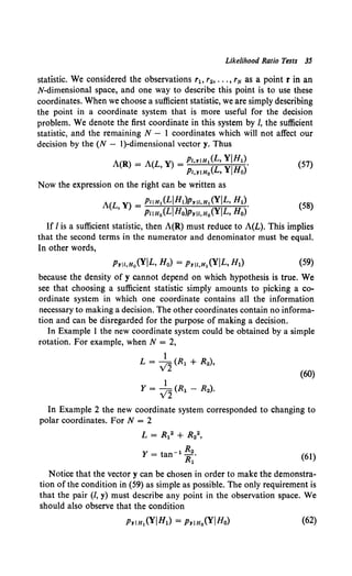
Now, if all the costs and a priori probabilities are known, we can find a
Bayes test. In Fig. 2.7a we plot the Bayes risk, .1ts(P1), as a function ofP1.
Observe that as P1 changes the decision regions for the Bayes test change
and therefore PF and PM change.
Now consider the situation in which a certain P1 (say P1 = Pr) is
assumed and the corresponding Bayes test designed. We now fix the
threshold and assume that P1is allowed to change. We denote the risk for
this fixed threshold test as j(APr, P1). Because the threshold is fixed, PF
and PM are fixed, and (44) is just a straight line. Because it is a Bayes test
for P1 = Pr, it touches the .1t8(P1) curve at that point. Looking at (14),
we see that the threshold changes continuously with P1. Therefore, when-
ever P1 =F Pr, the threshold in the Bayes test will be different. Because the
Bayes test minimizes the risk,
(45)

48. 32 2.2 Simple Binary Hypothesis Tests
(a) (b)
Cn
Coo
Coo
0~------7------;.. pl 0'--------'--- PI
(c) (d)
Fig. 2.7 Risk curves: (a) fixed risk versus typical Bayes risk; (b) maximum value of
.1t1 at P1 = 0.
If A is a continuous random variable with a probability distribution
function that is strictly monotonic, then changing TJ always changes the
risk. .'R.8 (P1) is strictly concave downward and the inequality in (45) is
strict. This case, which is one of particular interest to us, is illustrated in
Fig. 2.7a. We see that .'R.iPt, P1) is tangent to .'R.a(P1) at P1 = Pf, These
curves demonstrate the effect of incorrect knowledge of the a priori
probabilities.
An interesting problem is encountered if we assume that the a priori
probabilities are chosen to make our performance as bad as possible. In
other words, P1 is chosen to maximize our risk :JtF(Pt, P1). Three possible
examples are given in Figs. 2.7b, c, and d. In Fig. 2.7b the maximum of
:Jt8 (P1) occurs at P1 = 0. To minimize the maximum risk we use a Bayes
test designed assuming P1 = 0. In Fig. 2.7c the maximum of.'R.a(P1) occurs
at P1 = 1. To minimize the maximum risk we use a Bayes test designed
assuming P1 = 1. In Fig. 2.7d the maximum occurs inside the interval

49. Likelihood Ratio Tests 33
[0, 1], and we choose :RF to be the horizontal line. This implies that the
coefficient of P1 in (44) must be zero:
(Cll - Coo) + (Col - Cu)PM - (C1o - Coo)PF = 0. (46)
A Bayes test designed to minimize the maximum possible risk is called a
minimax test. Equation 46 is referred to as the minimax equation and is
useful whenever the maximum of :R8 (P1) is interior to the interval.
A special cost assignment that is frequently logical is
Coo= Cu = 0
(This guarantees the maximum is interior.)
Denoting,
the risk is,
Col= eM,
C1o = CF.
:RF = CFPF + Pl(CMPM - CFPF)
= PoCFPF + P1CMPM
and the minimax equation is
(47)
(48)
(49)
(50)
Before continuing our discussion oflikelihood ratio tests we shall discuss
a second criterion and prove that it also leads to a likelihood ratio test.
Neyman-Pearson Tests. In many physical situations it is difficult to
assign realistic costs or a priori probabilities. A simple procedure to by-
pass this difficulty is to work with the conditional probabilities PF and Pv.
In general, we should like to make PF as small as possible and Pv as large
as possible. For most problems of practical importance these are con-
flicting objectives. An obvious criterion is to constrain one of the prob-
abilities and maximize (or minimize) the other. A specific statement of this
criterion is the following:
Neyman-Pearson Criterion. Constrain PF = a.' ::::; a. and design a test to
maximize Pv (or minimize PM) under this constraint.
The solution is obtained easily by using Lagrange multipliers. We con-
struct the function F,
(51)
or
F = fzo PriH1 (RIHl) dR + , [{1
PriHo(RIHo) dR- a.']• (52)
Clearly, if PF = a.', then minimizing F minimizes PM.

50. 34 2.2 Simple Binary Hypothesis Tests
or
F = .(I -a')+ f [Pr!H1 (RIH1)- APriHo(RIHo)] dR. (53)
Jzo
Now observe that for any positive value of, an LRT will minimize F.
(A negative value of, gives an LRT with the inequalities reversed.)
This follows directly, because to minimize F we assign a point R to Z0
only when the term in the bracket is negative. This is equivalent to the test
Pr!H1 (RIHI) ,
PriHo(RIHo) < '
assign point to Z0 or say H0 • (54)
The quantity on the left is just the likelihood ratio. Thus F is minimized
by the likelihood ratio test
H1
A(R) ~ ,.
Ho
(55)
To satisfy the constraint we choose , so that PF = a'. If we denote the
density of A when H0 is true as PA!Ho(AIH0), then we require
PF = L"'PAIHo(AIHo) dA = a'. (56)
Solving (56) for ,gives the threshold. The value of, given by {56) will be
non-negative because PAIHo(AIHo) is zero for negative values of,. Observe
that decreasing , is equivalent to increasing Z1 , the region where we say
H1 • Thus Pv increases as , decreases. Therefore we decrease , until we
obtain the largest possible a' =:;; a. In most cases of interest to us PF is a
continuous function of, and we have PF = a. We shall assume this con-
tinuity in all subsequent discussions. Under this assumption the Neyman-
Pearson criterion leads to a likelihood ratio test. On p. 41 we shall see the
effect of the continuity assumption not being valid.
Summary. In this section we have developed two ideas of fundamental
importance in hypothesis testing. The first result is the demonstration that
for a Bayes or a Neyman-Pearson criterion the optimum test consists of
processing the observation R to find the likelihood ratio A(R) and then
comparing A(R) to a threshold in order to make a decision. Thus, regard-
less of the dimensionality of the observation space, the decision space is
one-dimensional.
The second idea is that ofa sufficient statistic /(R). The idea ofa sufficient
statistic originated when we constructed the likelihood ratio and saw that
it depended explicitly only on /(R). If we actually construct A(R) and then
recognize /(R), the notion of a sufficient statistic is perhaps of secondary
value. A more important case is when we can recognize /(R) directly. An
easy way to do this is to examine the geometric interpretation ofa sufficient

51. Likelihood Ratio Tests 3S
statistic. We considered the observations r1o r2, ••• , rN as a point r in an
N-dimensional space, and one way to describe this point is to use these
coordinates. When we choose a sufficient statistic, we are simply describing
the point in a coordinate system that is more useful for the decision
problem. We denote the first coordinate in this system by /, the sufficient
statistic, and the remaining N - I coordinates which will not affect our
decision by the (N - I)-dimensional vector y. Thus
A(R) = A(L Y) = PI,YiHl(L, YIHl). (57)
' PI,YIHo(L, YIHo)
Now the expression on the right can be written as
A(L Y) _ PliH1(LiHl)PYii,H1(YIL, H1).
' - PliH0 (LIHo)PYII,Ho(YIL, Ho)
(58)
If I is a sufficient statistic, then A(R) must reduce to A(L). This implies
that the second terms in the numerator and denominator must be equal.
In other words,
(59)
because the density of y cannot depend on which hypothesis is true. We
see that choosing a sufficient statistic simply amounts to picking a co-
ordinate system in which one coordinate contains all the information
necessary to making a decision. The other coordinates contain no informa-
tion and can be disregarded for the purpose of making a decision.
In Example 1 the new coordinate system could be obtained by a simple
rotation. For example, when N = 2,
1
L = v'2' (R1 + R2),
(60)
1
Y = v'2' (R1 - R2).
In Example 2 the new coordinate system corresponded to changing to
polar coordinates. For N = 2
L = R12 + R22,
y = tan-1 R2.
~ ~I)
Notice that the vector y can be chosen in order to make the demonstra-
tion of the condition in (59) as simple as possible. The only requirement is
that the pair (/, y) must describe any point in the observation space. We
should also observe that the condition
PYiH1(YIH1) = PYIHo(YIHo) (62)

52. J6 2.2 Simple Binary Hypothesis Tests
does not imply (59) unless I and y are independent under H1 and H0•
Frequently we will choose y to obtain this independence and then use (62)
to verify that I is a sufficient statistic.
2.2.2 Performance: Receiver Operating Characteristic
To complete our discussion of the simple binary problem we must
evaluate the performance of the likelihood ratio test. For a Neyrnan-
Pearson test the values of PF and PD completely specify the test perform-
ance. Looking at (42) we see that the Bayes risk .'R.8 follows easily ifPF and
PD are known. Thus we can concentrate our efforts on calculating PF and
PD.
We begin by considering Example I in Section 2.2.1.
Example I. From (25) we see that an equivalent test is
1 N H1 a VNm
I=--=- L R, ~ -=-ln'l + --·
VNat=l HoVNm 2a
(63)
u -../Nm In 11 d
Threshold: -./Nm In 'II + 2<1 = d + 2
(a)
(b)
Fig. 1.8 Error probabilities: (a) PF calculation; (b) Pv calculation.

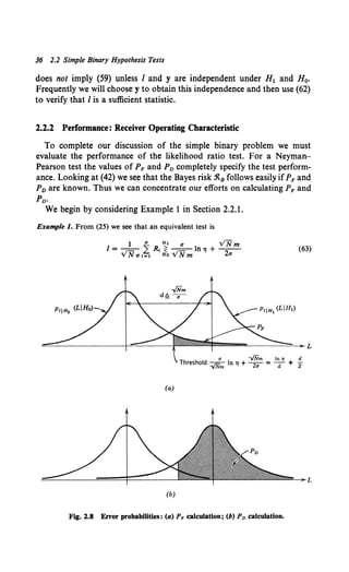
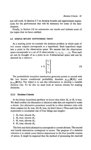
53. Performance: Receiver Operating Characteristic 37
We have multiplied (25) by a/VN m to normalize the next calculation. Under H 0,
1is obtained by adding N independent zero-mean Gaussian variables with variance
a2 and then dividing by VN a. Therefore I is N(O, 1).
Under H, I is N(VN m/a, 1). The probability densities on the two hypotheses are
sketched in Fig. 2.8a. The threshold is also shown. Now, P, is simply the integral of
PIIHo<LIHo) to the right of the threshold.
Thus
P, = --= exp -- dx,
i... 1 ( x2)
<m•>ld+d/2 v2'" 2
where d £ VN mfa is the distance between the means of the two densities.
integral in (64) is tabulated in many references (e.g., [3] or [4]).
We generally denote
err. (X)!!!. r...v~'" exp ( -t) dx,
where err. is an abbreviation for the error functiont and
f... 1 ( x2
)
errc. (X)!!!. x v2'" exp - 2 dx
is its complement. In this notation
(ln'l ~
P, = erfc• d + 1.)"
(64)
The
(65)
(66)
(67)
Similarly, Po is the integral of p,1H 1(LIH1) to the right of the threshold, as shown in
Fig. 2.8b:
i., 1 [ (x - d)2]
Po= --=exp dx
em •>ld+d/2 v2'" 2
= --=exp -- dy !!!_ errc. - - - .
i., 1 ( y2
) (In "' V
(ID.)/d-d/2 V2'1T 2 d 2
(68)
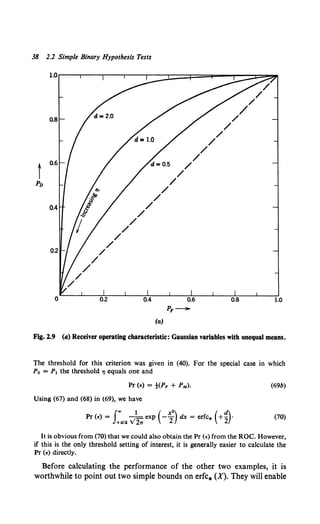
In Fig. 2.9a we have plotted Po versus P, for various values ofdwith 'I as the varying
parameter. For 'I = O,ln 'I = -oo, and the processor always guesses H1• Thus P, = 1
and Po = l. As"' increases, P, and Po decrease. When"' = oo, the processor always
guesses Ho and P, = Po = 0.
As we would expect from Fig. 2.8, the performance increases monotonically with d.
In Fig. 2.9b we have replotted the results to give Po versus d with P, as a parameter
on the curves. For a particular d we can obtain any point on the curve by choosing 'I
appropriately (0 :5 ., :5 oo).
The result in Fig. 2.9a is referred to as the receiver operating characteristic (ROC).
It completely describes the performance of the test as a function of the parameter of
interest.
A special case that will be important when we look at communication systems is
the case in which we want to minimize the total probability of error
(69a)
t The function that is usually tabulated is erf (X) = v2/'" J: exp (-y2) dy, which is
related to (65) in an obvious way.

54. 38 2.2 Simple Binary Hypothesis Tests
(a)
Fig. 2.9 (a) Receiver operating characteristic: Gaussian variables with unequal means.
The threshold for this criterion was given in (40). For the special case in which
Po = P1 the threshold 'I equals one and
Pr <~> = !(P, + PM>·
Using (67) and (68) in (69), we have
Pr <~> = J"' 1 exp (- x2
) dx = erfc. (+~)·
+d/2 v21r 2 2
(69b)
(70)
It is obvious from (70) that we could also obtain the Pr (•) from the ROC. However,
if this is the only threshold setting of interest, it is generally easier to calculate the
Pr (~) directly.
Before calculating the performance of the other two examples, it is
worthwhile to point out two simple bounds on erfc* (X). They will enable

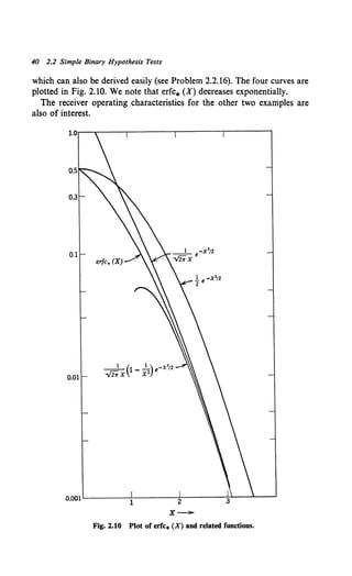
55. Performance: Receiver Operating Characteristic 39
us to discuss its approximate behavior analytically. For X > 0
1 ( 1 ) ( X2
) 1 ( x2)
V2rr X 1 - X2 exp -2 < erfc* (X) < V2rr Xexp -2 . (71)
This can be derived by integrating by parts. (See Problem 2.2.15 or Feller
(30].) A second bound is
erfc* (X) < -! exp (- ;
2
)• x > 0, (72)
d -
(b)
Fig. 2.9 (b) detection probability versus d.

56. 40 2.2 Simple Binary Hypothesis Tests
which can also be derived easily (see Problem 2.2.16). The four curves are
plotted in Fig. 2.10. We note that erfc* (X) decreases exponentially.
The receiver operating characteristics for the other two examples are
also of interest.
- - 1-- e-X/2
1 ( 1) 2
-.,(ii X X 2
x-
Fig. 2.10 Plot of erfc• (X) and related functions.

57. Performance: Receiver Operating Characteristic 41
Example 2. In this case the test is
(73)
The performance calculation for arbitrary N is somewhat tedious, so we defer it
until Section 2.6. A particularly simple case appearing frequently in practice is
N = 2. Under H 0 the r, are independent zero-mean Gaussian variables with variances
equal to ao2 :
P, = Pr (I~ yiHa) = Pr (r12 + r22 ~ YIHa). (74)
To evaluate the expression on the right, we change to polar coordinates:
r1 = zcos 8,
(75)
r2 = z sin 8,
Then
i2
" J"' 1 ( z•)
Pr (z2 ~ yiHa) = dB Z -
2 2 exp - -
2 2 dZ.
o ,f7 'ITao ao
(76)
Integrating with respect to 8, we have
f., 1 ( z•)
P, = Z 2 exp - -
2 2 dZ.
,f7 ao ao
(77)
We observe that /, the sufficient statistic, equals z2• Changing variables, we have
p, = f"' ~ exp (-~) dL = exp (-~)·
), 2a0 2ao 2ao
(Note that the probability density of the sufficient statistic is exponential.)
Similarly,
(78)
(79)
To construct the ROC we can combine (78) and (79) to eliminate the threshold y.
This gives
(80)
In terms of logarithms
(81)
As expected, the performance improves monotonically as the ratio a12 /ao2 increases.
We shall study this case and its generalizations in more detail in Section 2.6..
The two Poisson distributions are the third example.
Example 3. From (38), the likelihood ratio test is
~1 In TJ + m1 - mo
n lfo In m1 - In mo = y,
(82)
Because n takes on only integer values, it is more convenient to rewrite (82) as
Yr = 0, 1, 2, ... , (83)

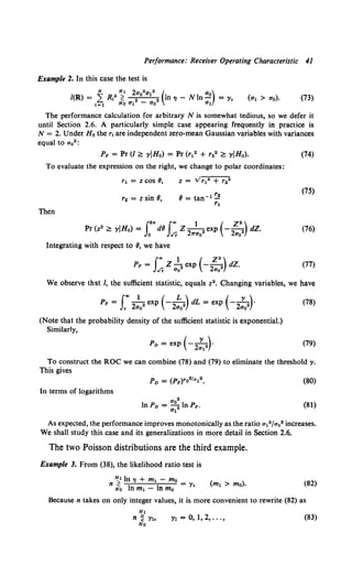
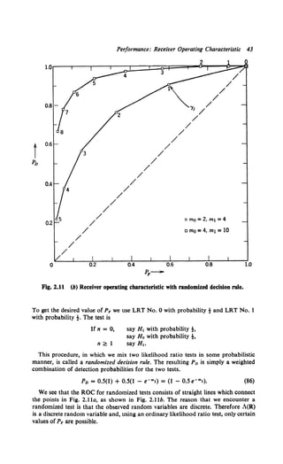
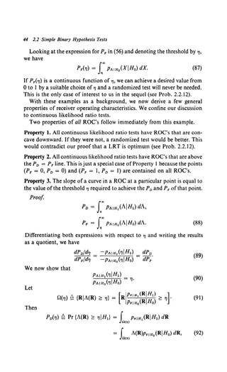
58. 42 2.2 Simple Binary Hypothesis Tests
where y1 takes on only integer values. Using (35),
YI = 0, 1, 2, ... , (84)
and from (36)
YI = 0, 1, 2, 0 0 oo (85)
The resulting ROC is plotted in Fig. 2.11a for some representative values of m0
and m1.
We see that it consists of a series of points and that PF goes from 1 to 1 - e-mo
when the threshold is changed from 0 to 1. Now suppose we wanted PF to have an
intermediate value, say 1 - te-mo. To achieve this performance we proceed in the
following manner. Denoting the LRT with y1 = 0 as LRT No. 0 and the· LRT with
Y1 = 1 as LRT No. 1, we have the following table:
0081-
[]
8
0.61-
Oo41-
Oo2~5
0
[]
7
o
4
[]
6
LRT
0
3
0
1
I
002
Y1
0
1
0
2
I
Oo4
PF-
Po
o mo = 2, m1 = 4
c mo =4, m1 =10
I I I
Oo6 008
Fig. 1.11 (a) Receiver operating characteristic, Poisson problem.
-
-
-
-
-
-
1.0

59. Performance: Receiver Operating Characteristic 43
/
/
/
/
/
/
/
/
/
/
/
/
/
/
/
/
/
/
/
/
/
/
/
/
/
/
0 mo= 2, ml=4
c mo =4, m1 =10
Fig. 2.11 (b) Receiver operating characteristic with randomized decision rule.
1.0
To get the desired value of P, we use LRT No. 0 with probability t and LRT No. 1
with probability t. The test is
If n = 0,
n ~ 1
say H1 with probability t,
say Ho with probability t,
say H1.
This procedure, in which we mix two likelihood ratio tests in some probabilistic
manner, is called a randomized decision rule. The resulting Po is simply a weighted
combination of detection probabilities for the two tests.
Po = 0.5(1) + 0.5(1 - e-ml) = (1 - O.S e-m1). (86)
We see that the ROC for randomized tests consists of straight lines which connect
the points in Fig. 2.lla, as shown in Fig. 2.llb. The reason that we encounter a
randomized test is that the observed random variables are discrete. Therefore A(R)
is a discrete random variable and, using an ordinary likelihood ratio test, only certain
values ofP, are possible.

60. 44 2.2 Simple Binary Hypothesis Tests
Looking at the expression for PF in (56) and denoting the threshold by "'•
we have
(87)
If PiTJ) is a continuous function of TJ, we can achieve a desired value from
0 to I by a suitable choice of TJ and a randomized test will never be needed.
This is the only case of interest to us in the sequel (see Prob. 2.2.12).
With these examples as a background, we now derive a few general
properties of receiver operating characteristics. We confine our discussion
to continuous likelihood ratio tests.
Two properties of all ROC's follow immediately from this example.
Property 1. All continuous likelihood ratio tests have ROC's that are con-
cave downward. If they were not, a randomized test would be better. This
would contradict our proof that a LRT is optimum (see Prob. 2.2.12).
Property 2. All continuous likelihood ratio tests have ROC's that are above
the PD = PFline. This is just a special case ofProperty l because the points
(PF = 0, PD = 0) and (PF = I, PD = 1) are contained on all ROC's.
Property 3. The slope of a curve in a ROC at a particular point is equal to
the value of the threshold TJ required to achieve the PD and PF of that point.
Proof.
PD = f"PAIHl(AIHl) dA,
PF = f'PAIHo(AIHo) dA. (88)
Differentiating both expressions with respect to TJ and writing the results
as a quotient, we have
dPDfdTJ -PAIH1 (7JIH1) dPD
dPFfdTJ = -PAIHo('IIHo) = dPF.
(89)
We now show that
Let
Then
(90)
n(TJ) £ {RIA(R) ~ 11} = (RI;::::~::z:~ ~ "~l (91)
PD(TJ) £ Pr {A(R) ~ TJIHl} = r PriHl(RIHl) dR
Jn<~>
= f A(R)pr1n0 (RIH0) dR, (92)
Jn<~>

61. Performance: Receiver Operating Characteristic 45
where the last equality follows from the definition of the likelihood ratio.
Using the definition of 0(7]), we can rewrite the last integral
Pv(TJ) = f A(R)Prlno(RIHo) dR = i"" XpAino(XiHo) dX. (93)
Jnc~> ~
Differentiating (93) with respect to 7J, we obtain
(94)
Equating the expression for dPv(n)fd7J in the numerator of (89) to the
right side of (94) gives the desired result.
We see that this result is consistent with Example I. In Fig. 2.9a, the
curves for nonzero d have zero slope at PF = Pv = 1 (71 = 0) and infinite
slope at PF = Pv = 0 (71 = oo).
Property 4. Whenever the maximum value of the Bayes risk is interior to
the interval (0, I) on the P1 axis, the minimax operating point is the
intersection of the line
(C11 - Coo) + (Col - C11)(l - Pv) - (C1o - Coo)PF = 0 (95)
and the appropriate curve of the ROC (see 46). In Fig. 2.12 we show the
special case defined by (50),
(96)
Fig. 2.12 Determination of minimax operating point.

62. 46 2.3 M Hypotheses
superimposed on the ROC of Example 1. We see that it starts at the point
PF = 0, PD = 1, and intersects the PF = 1 line at
PF = 1- cF.
eM (97)
This completes our discussion of the binary hypothesis testing problem.
Several key ideas should be re-emphasized:
1. Using either a Bayes criterion or a Neyman-Pearson criterion, we
find that the optimum test is a likelihood ratio test. Thus, regardless of the
dimensionality of the observation space, the test consists of comparing a
scalar variable A(R) with a threshold. (We assume PF("/) is continuous.)
2. In many cases construction of the LRT can be simplified if we can
identify a sufficient statistic. Geometrically, this statistic is just that
coordinate in a suitable coordinate system which describes the observation
space that contains all the information necessary to make a decision.
3. A complete description of the LRT performance was obtained
by plotting the conditional probabilities PD and PF as the threshold"' was
varied. The resulting ROC could be used to calculate the Bayes risk for
any set ofcosts. In many cases only one value of the threshold is of interest
and a complete ROC is not necessary.
A number of interesting binary tests are developed in the problems.
1.3 M HYPOTHESES
The next case of interest is one in which we must choose one of M
hypotheses. In the simple binary hypothesis test there were two source
outputs, each of which corresponded to a single hypothesis. In the simple
M-ary test there are M source outputs, each of which corresponds to one
of M hypotheses. As before, we assume that we are forced to make a
decision. Thus there are M 2 alternatives that may occur each time the
experiment is conducted. The Bayes criterion assigns a cost to each ofthese
alternatives, assumes a set of a priori probabilities P0 , P1, ••• , PM-h and
minimizes the risk. The generalization of the Neyman-Pearson criterion to
M hypotheses is also possible. Because it is not widely used in practice, we
shall discuss only the Bayes criterion in the text.
Bayes Criterion. To find a Bayes test we denote the cost of each course
of action as C11• The first subscript signifies that the ith hypothesis is
chosen. The second subscript signifies that thejth hypothesis is true. We
denote the region of the observation space in which we choose H1 as Z1

63. Bayes Criterion 47
and the a priori probabilities are P1• The model is shown in Fig. 2.13. The
expression for the risk is
3t = ~1
:'%P,CII Iz,Pr1H1(RIH,) dR. (98)
To find the optimum Bayes test we simply vary the Z, to minimize 3t.
This is a straightforward extension ofthe technique used in the binary case.
For simplicity of notation, we shall only consider the case in which M = 3
in the text.
Noting that Z0 = Z - Z1 - Z2, because the regions are disjoint, we
obtain
3t = PoCoo C PriHo(RIHo) dR + PoC1o C PriHo(RIHo)dR
Jz-z1-z2 Jz1
+ PoC2o C PriHo(RIHo) dR + P1Cu C PriH1 (RIHl)dR
Jz2 Jz-zo -z2
+ P1Co1 C Pr!H1 (RIH1) dR + P1C21 C Pr!H1 (RIH1) dR
Jzo Jz2
+ P2C22 C Pr!H2 (RIH2) dR + P2Co2 C Pr!H2 (RIH2) dR
Jz-zo -Z1 Jzo
+ P2C12 C Pr!H2 (RIH2) dR. (99)
Jzl
This reduces to
3t = PoCoo + P1Cu + P2C22
+ C [P2(Co2- C22)PriH2 (RIH2) + P1(Co1- Cu)PriH1 (RIHl)]dR
Jzo
+ C [Po(ClO- Coo)PriHo(RIHo) + P2(C12- C22)Pr!H2 (RIH2}]dR
Jz1
+ C [Po(C2o - Coo)Pr!Ho(RIHo} + P1(C21 - Cu)Pr!H1 (RIHl)] dR.
Jz2
(100)
As before, the first three terms represent the fixed cost and the integrals
represent the variable cost that depends on our choice of Z0 , Z~> and Z2 •
Clearly, we assign each R to the region in which the value of the integrand
is the smallest. Labeling these integrands /0(R), / 1(R), and /2(R), we have
the following rule:
if Io(R) < /1(R) and /2(R), choose Ho,
if /1(R) < /0(R) and /2(R), choose H 17 (101)
if /2(R) < /0(R) and /1(R), choose H2•

64. 48 2.3 M Hypotheses
Fig. 2.13 M hypothesis problem.
Say Ht
Z:
observation
space
We can write these terms in terms of likelihood ratios by defining
A (R) 1:::,. PrrH1(RIHl)
1 - PriHo(RIHo)'
A2(R) (;:: Pr1H2(RIH2).
PriHo(RIHo)
(102)
Using (102) in (100) and (101), we have
(103)
H2orH1
P2(Co2 - C22) A2(R) ~ Po(C2o - Coo) + P1(C21 - Col) A1(R), (104)
Ho orH1
We see that the decision rules correspond to three lines in the At. A2
plane. It is easy to verify that these lines intersect at a common point and
therefore uniquely define three decision regions, as shown in Fig. 2.I4.
The decision space is two-dimensional for the three-hypothesis problem.
It is easy to verify that M hypotheses always lead to a decision space
which has, at most, (M- I) dimensions.
Several special cases will be useful in our later work. The first is defined
by the assumptions
Coo = C11 = C22 = 0,
C11 = I, i I= j.
(106)
These equations indicate that any error is of equal importance. Looking
at (98), we see that this corresponds to minimizing the total probability of
error.

65. At{R)
Fig. 2.14 Decision space.
Substituting into (103)-(105), we have
H1 or H2
P1A1(R) ~ Po,
Ho or H2
H2 or H1
P2A2(R) ~ Po,
Ho or H1
H2 or Ho
P2A2(R) ~ P1A1(R).
H 1 or Ho
Ho
'----'-----+ A1{R)
Po/P1
(a)
lnPo/P2
----1--rit-:--=-=-~ln At (R)
lnPo/P1
Ho
(b)
Fig. 2.15 Decision spaces.
Bayes Criterion 49
(107)

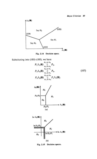
66. 50 2.3 M Hypotheses
The decision regions in the (A1o A2) plane are shown in Fig. 2.15a. In this
particular case, the transition to the (ln A1o ln A2) plane is straight-
forward (Fig. 2.15b). The equations are
Ht orH2 p
In A2(R) ~ In po' (108)
HoorHt 2
HoorH2 p
ln A2(R) ~ ln A1(R) + ln p1•
HoorHt 2
The expressions in (107) and (108) are adequate, but they obscure an
important interpretation of the processor. The desired interpretation is
obtained by a little manipulation.
Substituting (102) into (103-105) and multiplying both sides by
PriHo(RIHo), we have
Ht orH2
P1Pr1H1(RIH1) ~ PoPriHo(RIHo),
HoorH2
H2orH1
P2Pr1H2 (RIH2) ~ PoPriHo(RIHo),
HoorH1
(109)
H2orHo
P2Pr1H2 (RIH2) ~ P1Pr1H1 (RIH1).
Ht orHo
Looking at (109), we see that an equivalent test is to compute the a
posteriori probabilities Pr [H0 IR], Pr [H1IR], and Pr [H2IR1 and choose
the largest. (Simply divide both sides of each equation by p.(R) and
examine the resulting test.) For this reason the processor for the minimum
probability of error criterion is frequently referred to as a maximum a
posteriori probability computer. The generalization to M hypotheses is
straightforward.
The next two topics deal with degenerate tests. Both results will be useful
in later applications. A case of interest is a degenerate one in which we
combine H1 and H2• Then
C12 = C21 = o,
and, for simplicity, we can let
Col = C1o = C2o = Co2
and
Coo = Cu = C22 = 0.
Then (103) and (104) both reduce to
Ht orH2
P1A1(R) + P2A2(R) ~ Po
Ho
and (105) becomes an identity.
(110)
(Ill)
(112)
(113)

67. Po
p2
'----------~-+A1(R)
Po
pl
Fig. 2.16 Decision spaces.
Bayes Criterion 51
The decision regions are shown in Fig. 2.16. Because we have eliminated
all of the cost effect of a decision between H1 and H2, we have reduced it
to a binary problem.
We next consider the dummy hypothesis technique. A simple example
illustrates the idea. The actual problem has two hypotheses, H1 and H2,
but occasionally we can simplify the calculations by introducing a dummy
hypothesis H0 which occurs with zero probability. We let
P0 = 0,
and (114)
Substituting these values into (103-105), we find that (103) and (104)
imply that we always choose H1 or H2 and the test reduces to
Looking at (12) and recalling the definition of A1(R) and A2(R), we see
that this result is exactly what we would expect. [Just divide both sides of
(12) by Prrn0 (RIH0).] On the surface this technique seems absurd, but it
will turn out to be useful when the ratio
Prrn2 (RIH2)
Prrn,(R!Hl)
is difficult to work with and the ratios A1(R) and A2(R) can be made
simple by a proper choice ofPrrn0 (RIHo)·
In this section we have developed the basic results needed for the M-
hypothesis problem. We have not considered any specific examples

68. 52 2.4 Estimation Theory
because the details involved in constructing the likelihood ratios are the
same as those in the binary case. Typical examples are given in the
problems. Several important points should be emphasized.
1. The minimum dimension of the decision space is no more than
M - I. The boundaries of the decision regions are hyperplanes in the
(AI> ... , AM -1) plane.
2. The optimum test is straightforward to find. We shall find however,
when we consider specific examples that the error probabilities are
frequently difficult to compute.
3. A particular test of importance is the minimum total probability of
error test. Here we compute the a posteriori probability of each hypothesis
Pr (H;jR) and choose the largest.
These points will be appreciated more fully as we proceed through
various applications.
These two sections complete our discussion of simple hypothesis tests.
A case of importance that we have not yet discussed is the one in which
several source outputs are combined to give a single hypothesis. To study
this detection problem, we shall need some ideas from estimation theory.
Therefore we defer the composite hypothesis testing problem until Section
2.5 and study the estimation problem next.
2.4 ESTIMATION THEORY
In the last two sections we have considered a problem in which one of
several hypotheses occurred. As the result of a particular hypothesis, a
vector random variable r was observed. Based on our observation, we
shall try to choose the true hypothesis.
In this section we discuss the problem of parameter estimation. Before
formulating the general problem, let us consider a simple example.
Example 1. We want to measure a voltage a at a single time instant. From physical
considerations, we know that the voltage is between - V and + V volts. The measure-
ment is corrupted by noise which may be modeled as an independent additive zero-
mean Gaussian random variable n. The observed variable is r. Thus
r =a+ n. (116)
The probability density governing the observation process is p, 1a(RJA). In this case
1 ( (R- A)2)
Pria(RJA) = Pn(R - A) = ..;- exp - 2 2 •
21T Un O'n
(117)
The problem is to observe r and estimate a.
This example illustrates the basic features of the estimation problem.

69. Model 53
A model of the general estimation problem is shown in Fig. 2.17. The
model has the following four components:
Parameter Space. The output of the source is a parameter (or variable).
We view this output as a point in a parameter space. For the single-
parameter case, which we shall study first, this will correspond to segments
of the line -oo <A < oo. In the example considered above the segment is
(- V, V).
Probabilistic Mapping from Parameter Space to Observation Space. This
is the probability law that governs the effect of a on the observation.
Observation Space. In the classical problem this is a finite-dimensional
space. We denote a point in it by the vector R.
Estimation Rule. After observing R, we shall want to estimate the value
of a. We denote this estimate as a(R). This mapping of the observation
space into an estimate is called the estimation rule. The purpose of this
section is to investigate various estimation rules and their implementations.
The second and third components are familiar from the detection prob-
lem. The new features are the parameter space and the estimation rule.
When we try to describe the parameter space, we find that two cases arise.
In the first, the parameter is a random variable whose behavior is governed
by a probability density. In the second, the parameter is an unknown
quantity but not a random variable. These two cases are analogous to the
A
Probabilistic
mapping to
observation space
Parameter
space
Observation
space
Fig. 2.17 Estimation model.
I
I
I
I Estimation
rule

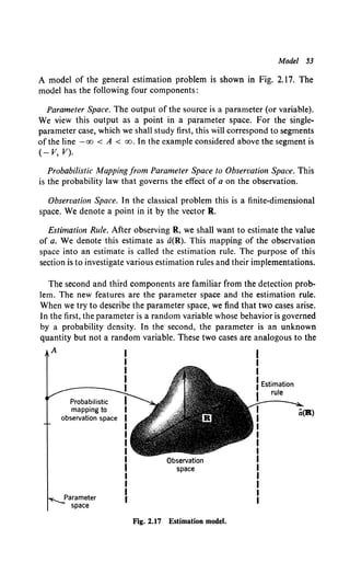
70. 54 2.4 Estimation Theory
source models we encountered in the hypothesis-testing problem. To corre-
spond with each of these models of the parameter space, we shall develop
suitable estimation rules. We start with the random parameter case.
2.4.1 Random Parameters: Bayes Estimation
In the Bayes detection problem we saw that the two quantities we had
to specify were the set of costs C!i and the a priori probabilities P1• The
cost matrix assigned a cost to each possible course of action. Because there
were M hypotheses and M possible decisions, there were M 2 costs. In
the estimation problem aand d(R) are continuous variables. Thus we must
assign a cost to all pairs [a, a(R)] over the range of interest. This is a
function of two variables which we denote as C(a, a). In many cases of
interest it is realistic to assume that the cost depends only on the error of
the estimate. We define this error as
a.(R) ~ a(R) - a. (118)
The cost function C(a.) is a function of a single variable. Some typical
cost functions are shown in Fig. 2.18. In Fig. 2.18a the cost function is
simply the square of the error:
(119)
This cost is commonly referred to as the squared error cost function. We
see that it accentuates the effects of large errors. In Fig. 2.1 8b the cost
function is the absolute value of the error:
C(a.) = ia.i. (120)
In Fig. 2.18c we assign zero cost to all errors less than ±ll./2. In other
words, an error less than fl/2 in magnitude is as good as no error. If
a. > fl/2, we assign a uniform value:
C(a.) = 0,
!l
ia.i :::;; 2'
ll.
(121)
= l, ia.i > 2"
In a given problem we choose a cost function to accomplish two
objectives. First, we should like the cost function to measure user satis-
faction adequately. Frequently it is difficult to assign an analytic measure
to what basically may be a subjective quality.
Our goal is to find an estimate that minimizes the expected value of the
cost. Thus our second objective in choosing a cost function is to assign one
that results in a tractable problem. In practice, cost functions are usually
some compromise between these two objectives. Fortunately, in many

71. Random Parameters: Bayes Estimation 55
(a)
C(A.)
--------~~------~A.
(b) (c)
Fig. 2.18 Typical cost functions: (a) mean-square error; (b) absolute error; (c) uniform
cost function.
problems of interest the same estimate will be optimum for a large class of
cost functions.
Corresponding to the a priori probabilities in the detection problem, we
have an a priori probability density p4 (A) in the random parameter estima-
tion problem. In all of our discussions we assume that p4 (A) is known. If
p4 (A) is not known, a procedure analogous to the minimax test may be
used.
Once we have specified the cost function and the a priori probability, we
may write an expression for the risk:
.1t ~ E{C[a, a(R)]} = s:"' dA s:"' C[A, d(R)lPa,r(A,R)dR. (122)
The expectation is over the random variable a and the observed variables
r. For costs that are functions of one variable only (122) becomes
.1t = s:"' dA s:"' C[A - a(R)]pa,r(A, R) dR. (123)

72. 56 2.4 Estimation Theory
The Bayes estimate is the estimate that minimizes the risk. It is straight-
forward to find the Bayes estimates for the cost functions in Fig. 2.18.
For the cost function in Fig. 2.18a, the risk corresponds to mean-square
error. We denote the risk for the mean-square error criterion as .1tms·
Substituting (I 19) into (123), we have
.1tms = J:.., dA J:.., dR[A - a(R)]2p11,r(A, R). (124)
The joint density can be rewritten as
Pa.r(A, R) = Pr(R)Palr(AJR). (125)
Using (125) in (124), we have
.1tms = J:.., dRpr(R) J:.., dA[A- a(R)]2p,. 1r(AJR). (126)
Now the inner integral and Pr(R) are non-negative. Therefore we can
minimize .1tms by minimizing the inner integral. We denote this estimate
Oms(R). To find it we differentiate the inner integral with respect to a(R)
and set the result equal to zero:
~ J:.., dA[A - a(R)]2Palr(AJR)
= -2 J:.., APalr(AJR)dA + 2a(R) J:..,Palr(AJR)dA. (127)
Setting the result equal to zero and observing that the second integral
equals I, we have
(128)
This is a unique minimum, for the second derivative equals two. The term
on the right side of (128) is familiar as the mean of the a posteriori density
(or the conditional mean).
Looking at (126), we see that if a(R) is the conditional mean the inner
integral is just the a posteriori variance (or the conditional variance).
Therefore the minimum value of .1tms is just the average of the conditional
variance over all observations R.
To find the Bayes estimate for the absolute value criterion in Fig. 2.18b
we write
:R.abs = J:.., dRpr(R) I:IX) dA[JA - a(R)i1Palr(AJR). (129)
To minimize the inner integral we write
[
(R) l..,
/(R) = dA[a(R)- A]p,. 1r(AJR) + dA[A- a(R)]Palr(AJR).
-oo 4<R)
(130)

73. Random Parameters: Bayes Estimation 57
Differentiating with respect to a(R) and setting the result equal to zero,
we have
Jdabs{R) lao
dApalr(AIR) = dApalr(AIR).
-co ~bs!W
(131)
This is just the definition of the median of the a posteriori density.
The third criterion is the uniform cost function in Fig. 2.18c. The risk
expression follows easily:
fao [ l4unrCR) +A/2 ]
.'ltunr = dRp.(R) I - Pair(AIR) dA .
- ao 4unr(R)-A/2
(132)
To minimize this equation we maximize the inner integral. Of particular
interest to us is the case in which ~ is an arbitrarily small but nonzero
number. A typical a posteriori density is shown in Fig. 2.19. We see that
for small ~ the best choice for u(R) is the value of A at which the a
posteriori density has its maximum. We denote the estimate for this
special case as amaiR), the maximum a posteriori estimate. In the sequel
we use t1map(R) without further reference to the uniform cost function.
To find clmap we must have the location of the maximum ofPair(AIR).
Because the logarithm is a monotone function, we can find the location of
the maximum of lnpa1
.(AIR) equally well. As we saw in the detection
problem, this is frequently more convenient.
Ifthe maximum is interior to the allowable range of A and lnpa1r(AIR)
has a continuous first derivative then a necessary, but not sufficient,
condition for a maximum can be obtained by differentiating In Pa1.(AIR)
with respect to A and setting the result equal to zero:
alnpai•<AIR)I = o.
oA A~a{R)
(133)
Pair (AiR)
Fig. 2.19 An a posteriori density.

74. 58 2.4 Estimation Theory
We refer to (133) as the MAP equation. In each case we must check to see
if the solution is the absolute maximum.
We may rewrite the expression for Pa1r(A IR) to separate the role of the
observed vector R and the a priori knowledge:
P (AIR) = Prla(RIA)pa(A), (134)
air Pr(R)
Taking logarithms,
lnpalr(AIR) = lnprla(RIA) + lnpa(A) -In Pr(R). (135)
For MAP estimation we are interested only in finding the value of A
where the left-hand side is maximum. Because the last term on the right-
hand side is not a function of A, we can consider just the function
/(A)~ lnprla(RIA) + Inpa(A). (136)
The first term gives the probabilistic dependence of R on A and the
second describes a priori knowledge.
The MAP equation can be written as
ol(A)i =olnpr1a(RIA)I +oinpa(A)i =O 037)
8A A=<i(R) 8A A=<i(R) 8A A=<i(R) •
Our discussion in the remainder ofthe book emphasizes minimum mean-
square error and maximum a posteriori estimates.
To study the implications of these two estimation procedures we
consider several examples.
Example 2. Let
i = 1, 2, ... , N. (138)
We assume that a is Gaussian, N(O, a.), and that the n, are each independent
Gaussian variables N(O, an). Then
N 1 ( (R - A)2)
Prla(RIA) = f1 _
1- - exp - '2 2 •
I= 1 V 21T On On
(139)
p.(A) = __!_ exp (- A
2
2)·
V21T a. 2aa
To find Ums(R) we need to know Palr(AIR). One approach is to find Pr(R) and
substitute it into (134), but this procedure is algebraically tedious. It is easier to
observe that p. 1r(AIR) is a probability density with respect to a for any R. Thus Pr(R)
just contributes to the constant needed to make
r.,P•I•(AIR)dA = 1. (140)
(In other words, Pr(R) is simply a normalization constant.) Thus
[( N 1 ) 1 ] { [ N J}
n----=- ----=- I (R, - A>·
(AIR) _ t=1 V21T an V21T a0 _! !=1 A2 •
Pair - (R) exp 2 2 + 2
Pr an Ua
(141)

75. Random Parameters: Bayes Estimation 59
Rearranging the exponent, completing the square, and absorbing terms depending
only on R,2 into the constant, we have
(142)
where
(143)
is the a posteriori variance.
We see that p. 1r(AIR) is just a Gaussian density. The estimate dms(R) is just the
conditional mean
(144)
Because the a posteriori variance is not a function of R, the mean-square risk
equals the a posteriori variance (see (126)).
Two observations are useful:
1. The R, enter into the a posteriori density only through their sum. Thus
N
/(R) = 2: R, (145)
lal
is a sufficient statistic. This idea of a sufficient statistic is identical to that in the
detection problem.
2. The estimation rule uses the information available in an intuitively logical
manner. If a0 2 « an2 /N, the a priori knowledge is much better than the observed data
and the estimate is very close to the a priori mean. (In this case, the a priori mean is
zero.) On the other hand, if a.2 » an2 /N, the a priori knowledge is of little value and
the estimate uses primarily the received data. In the limit dm• is just the arithmetic
average of the R,.
(146)
The MAP estimate for this case follows easily. Looking at (142), we see that because
the density is Gaussian the maximum value of p. 1r(AIR) occurs at the conditional
mean. Thus
(147)
Because the conditional median of a Gaussian density occurs at the conditional
mean, we also have
(148)
Thus we see that for this particular example all three cost functions in
Fig. 2.18 lead to the same estimate. This invariance to the choice of a cost
function is obviously a useful feature because of the subjective judgments
that are frequently involved in choosing C(aE). Some conditions under
which this invariance holds are developed in the next two properties.t
t These properties are due to Sherman [20]. Our derivation is similar to that given
by Viterbi [36].

76. 60 2.4 Estimation Theory
Property 1. We assume that the cost function C(a,) is a symmetric, convex-
upward function and that the a posteriori density Pa 1.(AIR) is symmetric
about its conditional mean; that is,
C(a,) = C(-a,) (symmetry), (149)
C(bx1 + (I - b)x2) s bC(x1) + (1 - b) C(x2) (convexity) (150)
for any b inside the range (0, 1) and for all x1 and x2• Equation 150 simply
says that all chords lie above or on the cost function.
This condition is shown in Fig. 2.20a. Ifthe inequality is strict whenever
x1 ¥- x2 , we say the cost function is strictly convex (upward). Defining
z ~ a - elms = a - E[aiR]
the symmetry of the a posteriori density implies
Pzir(ZIR) = Pz1•( -ZIR).
(151)
(152)
The estimate athat minimizes any cost function in this class is identical
to Oms (which is the conditional mean).
(a)
(b)
Fig. 2.20 Symmetric convex cost functions: (a) convex; (b) strictly convex.

77. Random Parameters: Bayes Estimation 61
Proof As before we can minimize the conditional risk [see (126)].
Define
.'ltB(aiR) ~ Ea[C(a- a)iR] = Ea[C(a- a)IR], (153)
where the second equality follows from (149). We now write four equivalent
expressions for .'R.8 (aR):
.'R.a(aR) = J:oo C(a - ams - Z)Pz!r(ZR) dZ
[Use (151) in (153)]
= J:oo C(a- Oms+ Z)Pz!r(ZiR) dZ
[(152) implies this equality]
= J:oo C(ams - a - Z)pz1r(ZIR) dZ
[(149) implies this equality]
= J:oo C(ams- a+ Z)pz1r(ZR) dZ
[(152) implies this equality].
(154)
(155)
(156)
(157)
We now use the convexity condition (150) with the terms in (155) and
(157):
.1{8 (aR) = tE({C[Z + (ams - a)] + C[Z - (ams - a)]}R)
~ E{C[t(Z + (ams - a)) + !(Z - (ams - a))]R}
= E[C(Z)R]. (158)
Equality will be achieved in (I 58) if Oms = a. This completes the proof.
If C(a,) is strictly convex, we will have the additional result that the
minimizing estimate a is unique and equals ams·
To include cost functions like the uniform cost functions which are not
convex we need a second property.
Property 2. We assume that the cost function is a symmetric, nondecreasing
function and that the a posteriori density Pa!r(AR) is a symmetric (about
the conditional mean), unimodal function that satisfies the condition
lim C(X)Pa!r(xiR) = 0.
x-oo
The estimate athat minimizes any cost function in this class is identical to
Oms· The proof of this property is similar to the above proof [36].

78. 62 2.4 Estimation Theory
The significance of these two properties should not be underemphasized.
Throughout the book we consider only minimum mean-square and maxi-
mum a posteriori probability estimators. Properties 1 and 2 ensure that
whenever the a posteriori densities satisfy the assumptions given above the
estimates that we obtain will be optimum for a large class ofcost functions.
Clearly, if the a posteriori density is Gaussian, it will satisfy the above
assumptions.
We now consider two examples of a different type.
Example 3. The variable a appears in the signal in a nonlinear manner. We denote
this dependence by s(A). Each observation r, consists of s(A) plus a Gaussian random
variable n., N(O, an). The n, are statistically independent of each other and a. Thus
r1 = s(A) + n1• (159)
Therefore
I ~~ [R, - s(A)]• A•
( {
N } )
Palr(AJR) = k(R) exp -Z - an• + a.• · (160)
This expression cannot be further simplified without specifying s(A) explicitly.
The MAP equation is obtained by substituting (160) into (137)
a 2 N os(A)'
Omap(R) = --; L [R, - s(A)] 8A . .
an iz: 1 A= amap(R)
(161)
To solve this explicitly we must specify s(A). We shall find that an analytic solution
is generally not possible when s(A) is a nonlinear function of A.
Another type of problem that frequently arises is the estimation of a
parameter in a probability density.
Example 4. The number of events in an experiment obey a Poisson law with mean
value a. Thus
An
Pr(nevents Ia= A)= 1 exp(-A), n = 0, 1,.... (162)
n.
We want to observe the number of events and estimate the parameter a of the Poisson
law. We shall assume that a is a random variable with an exponential density
Pa(A) = {" exp (-.A),
0,
The a posteriori density of a is
A> 0,
elsewhere.
(AJN) = Pr (n = N I a = A)p.(A).
Pain Pr (n = N)
Substituting (162) and (163) into (164), we have
Paln(AJN) = k(N)[AN exp (- A(l + ,))],
where
(163)
(164)
A~ 0, (165)
(166)

79. Random Parameters: Bayes Estimation 63
in order for the density to integrate to 1. (As already pointed out, the constant is
unimportant for MAP estimation but is needed if we find the MS estimate by
integrating over the conditional density.)
The mean-square estimate is the conditional mean:
Oms(N) = (l +N~)N+l rAN+l exp [-A(l + ~)] dA
(1 + ~)N +1 ( 1 )
= (1 + ,)N +2 (N + 1) = , + 1 (N + 1). (167)
To find limap we take the logarithm of (165)
In Patn(AIN) = NInA - A(l + ~) + In k(N). (168)
By differentiating with respect to A, setting the result equal to zero, and solving, we
obtain
N
Omap(N} = l + ~·
Observe that Umap is not equal to Urns·
(169)
Other examples are developed in the problems. The principal results
of this section are the following:
l. The minimum mean-square error estimate (MMSE) is always
the mean of the a posteriori density (the conditional mean).
2. The maximum a posteriori estimate (MAP) is the value of A
at which the a posteriori density has its maximum.
3. For a large class of cost functions the optimum estimate is the
conditional mean whenever the a posteriori density is a unimodal
function which is symmetric about the conditional mean.
These results are the basis of most of our estimation work. As we study
more complicated problems, the only difficulty we shall encounter is the
actual evaluation of the conditional mean or maximum. In many cases of
interest the MAP and MMSE estimates will turn out to be equal.
We now turn to the second class ofestimation problems described in the
introduction.
2.4.2 Real (Nonrandom) Parameter Estimationt
In many cases it is unrealistic to treat the unknown parameter as a
random variable. The problem formulation on pp. 52-53 is still appro-
priate. Now, however, the parameter is assumed to be nonrandom, and
we want to design an estimation procedure that is good in some sense.
t The beginnings of classical estimation theory can be attributed to Fisher [5, 6, 7, 8].
Many discussions of the basic ideas are now available (e.g., Cramer [9]), Wilks [10],
or Kendall and Stuart [11 )).

80. 64 2.4 Estimation Theory
A logical first approach is to try to modify the Bayes procedure in the
last section to eliminate the average over Pa(A). As an example, consider a
mean-square error criterion,
.1t(A) ~ s:"" [d(R) - A]2 Prla(RiA) dR, (170)
where the expectation is only over R, for it is the only random variable in
the model. Minimizing .1t(A), we obtain
dms(R) = A. (171)
The answer is correct, but not of any value, for A is the unknown
quantity that we are trying to find. Thus we see that this direct approach
is not fruitful. A more useful method in the nonrandom parameter case
is to examine other possible measures of quality of estimation procedures
and then to see whether we can find estimates that are good in terms of
these measures.
The first measure of quality to be considered is the expectation of the
estimate
f+oo
E[d(R)] 0. _"" a(R) Pria(RIA) dR. (172)
The possible values of the expectation can be grouped into three classes
l. If E[d(R)] = A, for all values of A, we say that the estimate is un-
biased. This statement means that the average value of the estimates equals
the quantity we are trying to estimate.
2. If E[d(R)] = A + B, where B is not a function of A, we say that the
estimate has a known bias. We can always obtain an unbiased estimate by
subtracting B from a(R).
3. IfE[d(R)] = A + B(A), we say that the estimate has an unknown bias.
Because the bias depends on the unknown parameter, we cannot simply
subtract it out.
Clearly, even an unbiased estimate may give a bad result on a particular
trial. A simple example is shown in Fig. 2.21. The probability density of
the estimate is centered around A, but the variance of this density is large
enough that big errors are probable.
A second measure of quality is the variance of estimation error:
Var [a(R) - A] = E{[a(R) - A]2} - B2(A). (173)
This provides a measure of the spread of the error. In general, we shall
try to find unbiased estimates with small variances. There is no straight-
forward minimization procedure that will lead us to the minimum variance
unbiased estimate. Therefore we are forced to try an estimation procedure
to see how well it works.

81. Maximum Likelihood Estimation 65
-+---------'--------+-A(R>
A
Fig. 2.21 Probability density for an estimate.
Maximum Likelihood Estimation. There are several ways to motivate
the estimation procedure that we shall use. Consider the simple estimation
problem outlined in Example I. Recall that
r =A+ n,
v'- I
Pria(RIA) = ( 21T un)- 1 exp [- 2
- 2 (R- A)2].
O'n
(174)
(175)
We choose as our estimate the value of A that most likely caused a given
value of R to occur. In this simple additive case we see that this is the same
as choosing the most probable value of the noise (N = 0) and subtracting
it from R. We denote the value obtained by using this procedure as a
maximum likelihood estimate.
(176)
In the general case we denote the function p..1a(RIA), viewed as a
function of A, as the likelihood function. Frequently we work with the
logarithm, lnp..1a(RIA), and denote it as the log likelihood function. The
maximum likelihood estimate am1(R) is that value of A at which the likeli-
hood function is a maximum. Ifthe maximum is interior to the range of A,
and In Pr1a{RI A) has a continuous first derivative, then a necessary con-
dition on am1
(R) is obtained by differentiating ln p..1
a(RIA) with respect to
A and setting the result equal to zero:
atnp..ja<RIA>I = o. (177)
oA A=4m,<R>
This equation is called the likelihood equation. Comparing (137) and (177),
we see that the ML estimate corresponds mathematically to the limiting
case of a MAP estimate in which the a priori knowledge approaches zero.
In order to see how effective the ML procedure is we can compute the
bias and the variance. Frequently this is difficult to do. Rather than
approach the problem directly, we shall first derive a lower bound on the
variance on any unbiased estimate. Then we shall see how the variance of
am1(R) compares with this lower bound.

82. 66 2.4 Estimation Theory
Cramer-Rao Inequality: Nonrandom Parameters. We now want to con-
sider the variance of any estimate a(R) of the real variable A. We shall
prove the following statement.
Theorem. (a) If a(R) is any unbiased estimate of A, then
var [a(R)- A];:: (E{[8lnp8A<R/A)f}rl (178)
or, equivalently,
(b)
Var [a(R)- A] ;:: { -E[82 ln-z~~(R/A)]}- 1
, (179)
where the following conditions are assumed to be satisfied:
(c)
8Prta(R/A) d 82p.,a(R/A)
oA an 8A2
exist and are absolutely integrable.
The inequalities were first stated by Fisher [6] and proved by Dugue [31 ].
They were also derived by Cramer [9] and Rao [12] and are usually
referred to as the Cramer-Rao bound. Any estimate that satisfies the
bound with an equality is called an efficient estimate.
The proof is a simple application of the Schwarz inequality. Because
a(R) is unbiased,
E[a(R) - A] ~ J:oo Prta(R/A)[a(R) - A] dR = 0. (180)
Differentiating both sides with respect to A, we have
d f<Xl
dA _"'p.1a(R/A)[a(R) - A] dR
f
<Xl 8
= _oo oA {p.1a(R/A)[a(R) - A]} dR = 0, (181)
where condition (c) allows us to bring the differentiation inside the integral.
Then
-J:oo p.1a(R/A) dR + J:oo op.,a<:/A) [a(R) - A] dR = 0. (182)
The first integral is just +1. Now observe that
8p.1a(RJA) _ 8lnp.1a(R/A) (R/A)
8A - 8A Prta . (183)

83. Cramer-Rao Inequality 67
Substituting (183) into (182), we have
J:oo 0 ln PB~(RIA)Pr1.,{RIA)[a(R) - A] dR = 1. (184)
Rewriting, we have
f~oo [olnpe~(RIA) v'pr1a(RIA)][vpr1
a(RIA)[a(R)- A]]dR = 1, (185)
and, using the Schwarz inequality, we have
{J~oo [a lnpa~(RIA)rPr,.,(RIA) dR}
x {f~oo [a(R) - A]2 Pr1
a(RIA) dR} ~ 1, {186)
where we recall from the derivation of the Schwarz inequality that equality
holds if and only if
aln pa~(RIA) = [a(R) _ A] k(A), {187)
for all Rand A. We see that the two terms of the left side of (186) are the
expectations in statement (a) of (178). Thus,
E{[d{R)- A]2} ~ {E[olnpa~(RiA)r}-1. (188)
To prove statement (b) we observe
(189)
Differentiating with respect to A, we have
foo opr,.,(RIA) dR = foo olnPrraCRIA) (RiA) dR = o (190)
-co oA -co oA Pria •
Differentiating again with respect to A and applying (183), we obtain
fco o2lnpr,.,(RIA) (RIA) dR
_co aA2 Prla
+ s:oo (olnp~~(RIA)r PrraCRIA)dR = 0 (191)
or
E[a2 lnpr,a(RIA)] = -E[alnpr,a(RIA)] 2
oA2 oA '
(192)
which together with (188) gives condition (b).

84. 68 2.4 Estimation Theory
Several important observations should be made about this result.
1. It shows that any unbiased estimate must have a variance greater
than a certain number.
2. If(187) is satisfied, the estimate dm1(R) will satisfy the bound with an
equality. We show this by combining (187) and (177). The left equality is
the maximum likelihood equation. The right equality is (187):
0 = olnp..,a(RIA)I = (a(R)- A) k(A)I . (193)
oA A:dm1(Rl A:dm1<Rl
In order for the right-hand side to equal zero either
a(R) = dm1(R)
or
(194)
(195)
Because we want a solution that depends on the data, we eliminate (195)
and require (194) to hold.
Thus, ifan efficient estimate exists, it is dm1(R) and can be obtained as a
unique solution to the likelihood equation.
3. If an efficient estimate does not exist [i.e., o lnpr 1a(RIA)joA cannot
be put into the form of (187)], we do not know how good Om1(R) is.
Further, we do not know how close the variance of any estimate will
approach the bound.
4. In order to use the bound, we must verify that the estimate ofconcern
is unbiased. Similar bounds can be derived simply for biased estimates
(Problem 2.4.17).
We can illustrate the application of ML estimation and the Cramer-Rao
inequality by considering Examples 2, 3, and 4. The observation model is
identical. We now assume, however, that the parameters to be estimated
are nonrandom variables.
Example 2. From (138) we have
i = 1, 2, ... , N.
Taking the logarithm of (139) and differentiating, we have
oln Prla(RIA) = ~ (.!._ ~ R, _A).
oA an N <=l
Thus
To find the bias we take the expectation of both sides,
} N } N
E[dm,(R)] = N 2 E(R,) = N 2 A = A,
i=- 1 t=l
so that dm,(R) is unbiased.
(196)
(197)
(198)
(199)

85. Nonrandom Parameter Estimation 69
Because the expression in (197) has the form required by (187), we know that
dm1(R) is an efficient estimate. To evaluate the variance we differentiate (197):
Using (179) and the efficiency result, we have
2
Var [dm1(R) - A] = uN.
Skipping Example 3 for the moment, we go to Example 4.
Example 4. Differentiating the logarithm of (162), we have
oIn Pr ~A= N IA) = o~ (N In A - A - InN!)
N 1
= A - 1 = A (N - A).
The ML estimate is
dm,(N) = N.
(200)
(201)
(202)
(203)
It is clearly unbiased and efficient. To obtain the variance we differentiate (202):
o2 In Pr (n = NjA) N
oA2 = - A2 • (204)
Thus
A2 A2
Var [cim1(N) - A] = E(N) = A = A. (205)
In both Examples 2 and 4 we see that the ML estimates could have been
obtained from the MAP estimates [let aa--+ oo in (144) and recall that
tims(R) = amap(R) and let A--+ 0 in (169)].
We now return to Example 3.
Example 3. From the first term in the exponent in (160), we have
o lnPrla(RIA) = _!, i [R, _ s(A)] os(A).
oA Un 1=1 oA
(206)
In general, the right-hand side cannot be written in the form required by (187), and
therefore an unbiased efficient estimate does not exist.
The likelihood equation is
[ os(A) ~] [.!. i Rl - s(A)]I = 0.
oA Un Nl=1 A=ami(R)
If the range of s(A) includes (1/N) L.f'=1 R., a solution exists:
1 N
s[dm,(R)] = N 2: R,.
1=1
If (208) can be satisfied, then
(207)
(208)
(209)

86. 70 2.4 Estimation Theory
[Observe that (209) tacitly assumes that s - 1( ·) exists. If it does not, then even in the
absence of noise we shall be unable to determine A unambiguously. Ifwe were designing
a system, we would always choose an s( ·) that allows us to find A unambiguously in
the absence of noise.]lf the range of s(a) does not include (1/N) L.f'~ 1 R, the maximum
is at an end point of the range.
We see that the maximum likelihood estimate commutes over nonlinear operations.
(This is not true for MS or MAP estimation.) If it is unbiased, we evaluate the bound
on the variance by differentiating (206):
o2 ln Prta(R[A) = ...!_ ~ [R _ (A)] o2s(A) _ .!!_ [os(A)] 2 · ( 210)
oA2 an2 ~~ ' s oA2 an2 oA
Observing that
E[r, - s(A)] = £(n1) = 0, (2ll)
we obtain the following bound for any unbiased estimate,
Var [a(R) - A] ;::: N[os(~;/oA]2 (212)
We see that the bound is exactly the same as that in Example 2 except for a factor
[os(A)/oA]2 • The intuitive reason for this factor and also some feeling for the con-
ditions under which the bound will be useful may be obtained by inspecting the
typical function shown in Fig. 2.22. Define
Y = s(A).
Then
(213)
(214)
The variance in estimating Y is just an2 /N. However, if y., the error in estimating Y,
is small enough so that the slope is constant, then
(215)
r=s(A)
:Y= J.r ~RJ___-~-r--
•=1 I v I
tn "E
I I ils(A) I
YA --+--L s(A)=s(AA)+(A-AA)--;u- +···
I A=~
I
s(A)
t
I
I
Fig. 2.22 Behavior of error variance in the presence of small errors.

87. Nonrandom Parameter Estimation 71
and
Var (y,) an2
Var (a,) ~ [Bs(A)/oA)2 = N[Bs(A)/BA]2•
(216)
We observe that if y, is large there will no longer be a simple linear relation between
y, and a,. This tells us when we can expect the Cramer-Rao bound to give an accurate
answer in the case in which the parameter enters the problem in a nonlinear manner.
Specifically, whenever the estimation error is small, relative to A B
2s(A)/BA2, we
should expect the actual variance to be close to the variance bound given by the
Cramer-Rao inequality.
The properties of the ML estimate which are valid when the error is
small are generally referred to as asymptotic. One procedure for developing
them formally is to study the behavior of the estimate as the number of
independent observations N approaches infinity. Under reasonably general
conditions the following may be proved (e.g., Cramer [9], pp. 500-504).
l. The solution ofthe likelihood equation (177) converges in probability
to the correct value of A as N-+ oo. Any estimate with this property is
called consistent. Thus the ML estimate is consistent.
2. The ML estimate is asymptotically efficient; that is,
1" Var [dm1(R) - A] l
N1~ ( -E [o2 ln~~~(RiA)])-l = ·
3. The ML estimate is asymptotically Gaussian, N(A, a.,,).
These properties all deal with the behavior of ML estimates for large N.
They provide some motivation for using the ML estimate even when an
efficient estimate does not exist.
At this point a logical question is: "Do better estimation procedures
than the maximum likelihood procedure exist?" Certainly if an efficient
estimate does not exist, there may be unbiased estimates with lower
variances. The difficulty is that there is no general rule for finding them.
In a particular situation we can try to improve on the ML estimate. In
almost all cases, however, the resulting estimation rule is more complex,
and therefore we emphasize the maximum likelihood technique in all of
our work with real variables.
A second logical question is: "Do better lower bounds than the Cramer-
Rao inequality exist?" One straightforward but computationally tedious
procedure is the Bhattacharyya bound. The Cramer-Rao bound uses
82pr1.,(RIA)/BA2• Whenever an efficient estimate does not exist, a larger
bound which involves the higher partial derivatives can be obtained.
Simple derivations are given in [13] and [14] and in Problems 2.4.23-24.
For the cases of interest to us the computation is too involved to make the
bound of much practical value. A second bound is the Barankin bound

88. 72 2.4 Estimation Theory
(e.g. [15]). Its two major advantages are that it does not require the
probability density to be differentiable and it gives the greatest lower
bound. Its disadvantages are that it requires a maximization over a
function to obtain the bound and the procedure for finding this maximum
is usually not straightforward. Some simple examples are given in the
problems (2.4.18-19). In most of our discussions, we emphasize the
Cramer-Rao bound.
We now digress briefly to develop a similar bound on the mean-square
error when the parameter is random.
Lower Boundon the Minimum Mean-Square Error in Estimating a Random
Parameter. In this section we prove the following theorem.
Theorem. Let a be a random variable and r, the observation vector. The
mean-square error of any estimate c:l(R) satisfies the inequality
E {[a(R) - a]2} ~ (E { [8ln PB~R, A)] 2})-1
= { -E[82 lnp;A~R, A)]}-1.
(217)
Observe that the probability density is a joint density and that the expecta-
tion is over both a and r. The following conditions are assumed to exist:
l. 8Pr.~<:· A) is absolutely integrable with respect to R and A.
2. 02PrB~~· A) is absolutely integrable with respect to R and A.
3. The conditional expectation of the error, given A, is
B(A) = f~oo [c:l(R) - A] Prla(RIA) dR.
We assume that
lim B(A) Pa(A) = 0,
lim B(A) Pa(A) = 0.
A-- oo
(218)
(219)
(220)
The proof is a simple modification of the one on p. 66. Multiply both
sides of (218) by Pa(A) and then differentiate with respect to A:
d f<X)
dA [Pa(A) B(A)] = - _oo Pr,a(R, A) dR
+ I<X) 8pr,a(R, A) [c:l(R) - A] dR. (221)
-<Xl oA

89. Nonrandom Parameter Estimation 73
Now integrate with respect to A:
Pa(A) B(A{: = -1 + s:"'s:"'opr,~~· A) [a(R) - A] dA dR. (222)
The assumption in Condition 3 makes the left-hand side zero. The
remaining steps are identical. The result is
E{[a(R)- a]2} ~ {E[(Olnpa~R,A)rn- 1
(223)
or, equivalently,
E{[a(R)- a]2} ~ { -£[82ln~~a2(RIA)] - £[82l~~~(A)]}-1 (224)
with equality if and only if
8ln pa~R, A) = k[a(R) - A], (225)
for all Rand all A. (In the nonrandom variable case we used the Schwarz
inequality on an integral over R so that the constant k(A) could be a
function of A. Now the integration is over both Rand A so that k cannot
be a function of A.) Differentiating again gives an equivalent condition
82 In Pr,a(R, A) = _ k
oA2 •
(226)
Observe that (226) may be written in terms of the a posteriori density,
82lnpa,lAIR) = -k
iJA2 . (227)
Integrating (227) twice and putting the result in the exponent, we have
(228)
for all R and A; but (228) is simply a statement that the a posteriori
probability density ofa must be Gaussian for all R in order for an efficient
estimate to exist. (Note that C1 and C2 are functions of R).
Arguing as in (193)-(195), we see that if (226) is satisfied the MAP
estimate will be efficient. Because the minimum MSE estimate cannot have
a larger error, this tells us that iims(R) = iimap(R) whenever an efficient
estimate exists. As a matter of technique, when an efficient estimate does
exist, it is usually computationally easier to solve the MAP equation than
it is to find the conditional mean. When an efficient estimate does not exist,
we do not know how closely the mean-square error, using either am.(R)
or iimap(R), approaches the lower bound. Asymptotic results similar to
those for real variables may be derived.

90. 74 2.4 Estimation Theory
2.4.3 Multiple Parameter Estimation
In many problems of interest we shall want to estimate more than one
parameter. A familiar example is the radar problem in which we shall
estimate the range and velocity ofa target. Most ofthe ideas and techniques
can be extended to this case in a straightforward manner. The model is
shown in Fig. 2.23. If there are K parameters, a~> a2, ••• , aK, we describe
them by a parameter vector a in a K-dimensional space. The other elements
of the model are the same as before. We shall consider both the case in
which a is a random parameter vector and that in which a is a real (or
nonrandom) parameter vector. Three issues are of interest. In each the
result is the vector analog to a result in the scalar case.
1. Estimation procedures.
2. Measures of error.
3. Bounds on performance.
(K-dimensional
estimate)
Fig. 2.23 Multiple parameter estimation model.

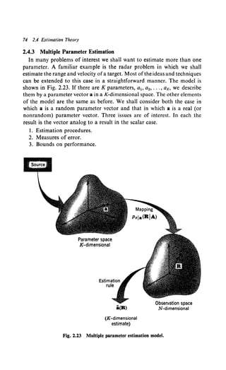
91. Multiple Parameter Estimation 15
Estimation Procedure. For random variables we could consider the
general case of Bayes estimation in which we minimize the risk for some
arbitrary scalar cost function C(a, i), but for our purposes it is adequate
to consider only cost functions that depend on the error. We define the
error vector as
[
al(R) - a1]
a,(R) = ~2(R) - a2 = a(R) - a.
aK(R)- aK
(229)
For a mean-square error criterion, the cost function is simply
K
C(a,(R)) ~ L a,1
2(R) = a/(R) a,(R). (230)
!= 1
This is just the sum of the squares of the errors. The risk is
co
-1tms = IIC(a,(R)) Pr,a(R, A) dR dA (231)
-co
or
As before, we can minimize the inner integral for each R. Because the
terms in the sum are positive, we minimize them separately. This gives
(233}
or
(234)
It is easy to show that mean-square estimation commutes over linear
transformations. Thus, if
b = Da,
where D is a L x K matrix, and we want to minimize
the result will be,
bms{R) = Dims{R)
[see Problem 2.4.20 for the proof of (237)].
(235)
(236)
{237)

92. 76 2.4 Estimation Theory
For MAP estimation we must find the value of A that maximizes
Palr(AIR). If the maximum is interior and olnpa1r(AIR)/8A; exists at the
maximum then a necessary condition is obtained from the MAP equations.
By analogy with (137) we take the logarithm of Pa1r(AIR), differentiate
with respect to each parameter A;, i = I, 2, ... , K, and set the result equal
to zero. This gives a set of K simultaneous equations:
aIn p;~<AIR)I = o, i = 1. 2, ... , K. (238)
! A~imap(R)
We can write (238) in a more compact manner by defining a partial
derivative matrix operator
0
oA1
0
VA?:::. oA2 (239)
0
oAK
This operator can be applied only to 1 x m matrices; for example,
(240)
Several useful properties of VA are developed in Problems 2.4.27-28.
In our case (238) becomes a single vector equation,
(241)
Similarly, for ML estimates we must find the value of A that maximizes
Pr1a(RIA). If the maximum is interior and olnpr1a(RIA)IoA; exists at the
maximum then a necessary condition is obtained from the likelihood
equations:
VA[ln Prla(RIA)]IA-am1
<R> = 0. (242)
In both cases we must verify that we have the absolute maximum.
Measures ofError. For nonrandom variables the first measure of interest
is the bias. Now the bias is a vector,
B(A) ?:::. E[a,(R)] = E[a(R)] - A. (243)

93. Multiple Parameter Estimation 77
Ifeach component of the bias vector is zero for every A, we say that the
estimate is unbiased.
In the single parameter case a rough measure of the spread of the error
was given by the variance of the estimate. In the special case in which
a,(R) was Gaussian this provided a complete description:
(244)
For a vector variable the quantity analogous to the variance is the
covariance matrix
E[(a, - a,)(a.T - a/)] ~ A., (245)
where
a, ~ E(a,) = B(A). (246)
The best way to determine how the covariance matrix provides a
measure of spread is to consider the special case in which the a,, are
jointly Gaussian. For algebraic simplicity we let E(a,) = 0. The joint
probability density for a set of K jointly Gaussian variables is
Pa,(A,) = (J27TJK12JA,JYz)- 1 exp (-1-A/A, - 1A,) (247)
(e.g., p. 151 in Davenport and Root [I]).
The probability density for K = 2 is shown in Fig. 2.24a. In Figs.
2.24b,c we have shown the equal-probability contours of two typical
densities.From (247) we observe that the equal-height contours are
defined by the relation,
(248)
which is the equation for an ellipse when K = 2. The ellipses move out
monotonically with increasing C. They also have the interesting property
that the probability of being inside the ellipse is only a function of C2 •
Property. For K = 2, the probability that the error vector lies inside an
ellipse whose equation is
is
P = 1 - exp (- ~}
Proof The area inside the ellipse defined by (249) is
A: = JA,J Yz7TC2.
(249)
(250)
(251)
The differential area between ellipses corresponding to C and C + dC
respectively is
(252)

94. 78 2.4 Estimation Theory
(b) (c)
Fig. 2.24 Gaussian densities: [a] two-dimensional Gaussian density; [b) equal-height
contours, correlated variables; [c] equal-height contours, uncorrelated variables.
The height of the probability density in this differential area is
(27TIA.IY.)- 1 exp (- ~2
)· (253)
We can compute the probability of a point lying outside the ellipse by
multiplying (252) by (253) and integrating from C to oo.
I - P = f' X exp (- ~2
) dX = exp ( - ;
2
), (254)
which is the desired result.

95. Multiple Parameter Estimation 79
For this reason the ellipses described by (248) are referred to as con-
centration ellipses because they provide a measure of the concentration of
the density.
A similar result holds for arbitrary K. Now, (248) describes an ellipsoid.
Here the differential volumet in K-dimensional space is
7TK/2
dv = IA.IY. r(K/2 + 1) KCK- 1 dC. (255)
The value of the probability density on the ellipsoid is
[(27T)K'21A.i Y.] -1 exp (- ~} (256)
Therefore
K ioo K-1 -x212
l - p = (2)K'2r(K/2 + 1) c X e dX, (257)
which is the desired result. We refer to these ellipsoids as concentration
ellipsoids.
When the probability density of the error is not Gaussian, the concen-
tration ellipsoid no longer specifies a unique probability. This is directly
analogous to the one-dimensional case in which the variance of a non-
Gaussian zero-mean random variable does not determine the probability
density. We can still interpret the concentration ellipsoid as a rough
measure of the spread of the errors. When the concentration ellipsoids of
a given density lie wholly outside the concentration ellipsoids of a second
density, we say that the second density is more concentrated than the first.
With this motivation, we derive some properties and bounds pertaining to
concentration ellipsoids.
Bounds on Estimation Errors: Nonrandom Variables. In this section we
derive two bounds. The first relates to the variance of an individual error;
the second relates to the concentration ellipsoid.
Property I. Consider any unbiased estimate of A1• Then
(258)
where Jti is the iith element in the K x K square matrix J- 1• The elements
in J are
J. !:::. E [8 In Prla(RIA). 8 In Prla(RIA)]
'' - 8A1 8A,
= -E[82 lnpr,a(RIA)]
oA1 aA,
t e.g., Cramer [9], p. 120, or Sommerfeld [32].
(259)

96. 80 2.4 Estimation Theory
or
J ~ E({VA[Jn Prla(RjA)]}{VA[ln Pr!a(RjA)JY)
= - E[VA({VA[Jn Prla(RjA)]V)].
(260)
The J matrix is commonly called Fisher's information matrix. The equality
in (258) holds if and only if
'(R) _A·=~ k-(A)8lnprla(RjA)
~ I ~ ~ 8A.
1 = 1 1
(261)
for aii values of At and R.
In other words, the estimation error can be expressed as the weighted
sum of the partial derivatives of In Pr1a(RjA) with respect to the various
parameters.
Proof Because dt(R) is unbiased,
I:"' [di(R) - A;] Pr!a(RjA) dR = 0
or
I:oo dt(R) Prla(RjA) dR = At.
Differentiating both sides with respect to Ai> we have
I:00 a,(R) OPri~~~IA) dR
= I"' '·(R) 8 In Pria(RjA) (RjA) dR = 8 .
a, oA. Pr1a tr
-CX) 1
We shall prove the result for i = 1. We define a K + l vector
a1(R)- A1
oIn Pr1a(RjA)
X=
--oA-
1
- -
The covariance matrix is
0
(262)
(263)
(264)
(265)
(266)

97. Multiple Parameter Estimation 81
[The ones and zeroes in the matrix follow from (264).] Because it is a
covariance matrix, it is nonnegative definite, which implies that the deter-
minant of the entire matrix is greater than or equal to zero. (This con-
dition is only necessary, not sufficient, for the matrix to be nonnegative
definite.)
Evaluating the determinant using a cofactor expansion, we have
u,1
2IJI - cofactor J11 ~ 0. (267)
If we assume that J is nonsingular, then
2 cofactor Ju _ Jll
u,, ~ IJI - ' (268)
which is the desired result. The modifications for the case when J is
singular follow easily for any specific problem.
In order for the determinant to equal zero, the term A1(R) - A1 must
be expressible as a linear combination of the other terms. This is the
condition described by (261). The second line of (259) follows from the
first line in a manner exactly analogous to the proof in (189)-(192). The
proof for i =f. I is an obvious modification.
Property 2. Consider any unbiased estimate of A. The concentration ellipse
lies either outside or on the bound ellipse defined by
A/JA, = C2•
(269)
(270)
Proof We shall go through the details for K = 2. By analogy with the
preceding proof, we construct the covariance matrix of the vector.
tit{R)- A1
d2(R)- A2
X= 8 In Pr!a(RIA)
8A1
(271)
8lnprla(RIA)
8A2
Then
2 I
0
ul. pul.u2. :
I
pu1.u2. 0"2.
2 I
0 1
I
I
E[xxT] = ---------------·--------
'
'
0 :Ju Jl2
[~J· (272)
I
0 :J21 J22

98. 82 2.4 Estimation Theory
The second equality defines a partition of the 4 x 4 matrix into four
2 x 2 matrices. Because it is a covariance matrix, it is nonnegative definite.
Using a formula for the determinant of a partitioned matrix,t we have
(273)
or, assuming that A. is nonsingular and applying the product rule for
determinants,
(274)
This implies
IJ - A.-ll ~ 0. (275)
Now consider the two ellipses. The intercept on the A,1 axis is
Al,21 = C2 IA~I
A2 , = o a2
(276)
for the actual concentration ellipse and
Al, 21 = C2_!_
A2 , =O Ju
(277)
for the bound ellipse.
We want to show that the actual intercept is greater than or equal to the
bound intercept. This requires
IuiA.I ~ a22 • (278)
This inequality follows because the determinant of the 3 x 3 matrix in
the upper left corner of (272) is greater than or equal to zero. (Otherwise
the entire matrix is not nonnegative definite, e.g. [16] or [18].) Similarly,
the actual intercept on the A2, axis is greater than or equal to the bound
intercept. Therefore the actual ellipse is either always outside (or on) the
bound ellipse or the two ellipses intersect.
If they intersect, we see from (269) and (270) that there must be a
solution, A., to the equation
or
In scalar notation
A1, 2 D11 + 2A1,A2,D12 + A2, 2 D22 = 0
or, equivalently,
t Bellman (16], p. 83.
(279)
(280)
(281)
(282)

99. Multiple Parameter Estimation 83
Solving for A1./A2., we would obtain real roots only if the discriminant
were greater than or equal to zero. This requires
(283)
The inequality is a contradiction of(275). One possibility is IJ- A. - 11= 0,
but this is true only when the ellipses coincide. In this case all the estimates
are efficient.
For arbitrary K we can show that J - A, - 1 is nonnegative definite.
The implications with respect to the concentration ellipsoids are the same
as forK= 2.
Frequently we want to estimate functions of the K basic parameters
rather than the parameters themselves. We denote the desired estimates
as
d1 = K<~1 (A),
d2 = g"2(A), (284)
dM = g<IM(A).
or
d = g..(A)
The number of estimates M is not related to K in general. The functions
may be nonlinear. The estimation error is
J, - g1(A) ~ d,,. (285)
If we assume that the estimates are unbiased and denote the error
covariance matrix as A., then by using methods identical to those above
we can prove the following properties.
Property 3. The matrix
(286)
is nonnegative definite.
This implies the following property Uust multiply the second matrix
out and recall that all diagonal elements of nonnegative definite matrix
are nonnegative):
Property 4.
V (d ) > ~ ~ 8g11,(A) JH oga,(A).
ar ., - "'7- 7 oA, OA, (287)
For the special case in which the desired functions are linear, the result
in (287) can be written in a simpler form.

100. 84 2.4 Estimation Theory
Property 5. Assume that
gd(A) Q GdA,
where Gd is an M x K matrix. If the estimates are unbiased, then
1., - GdJ -lGdT
is nonnegative definite.
(288)
Property 6. Efficiency commutes with linear transformations but does not
commute with nonlinear transformations. In other words, if ais efficient,
then d will be efficient if and only if gd(A) is a linear transformation.
Bounds on Estimation Errors: Random Parameters. Just as in the single
parameter case, the bound for random parameters is derived by a straight-
forward modification of the derivation for nonrandom parameters. The
information matrix now consists of two parts:
(289)
The matrix J0 is the information matrix defined in (260) and represents
information obtained from the data. The matrix JP represents the a priori
information. The elements are
J 6. E [8 In pa(A) 8 In Pa(A)]
PI! - oA1 oA,
= _ E [82
InPa(A)].
8A18A1
The correlation matrix of the errors is
R, Q E(a,a/).
(290}
(291)
The diagonal elements represent the mean-square errors and the off-
diagonal elements are the cross correlations. Three properties follow easily:
Property No. 1.
E[a,,2 ] ;:: N 1• (292)
In other words, the diagonal elements in the inverse of the total informa-
tion matrix are lower bounds on the corresponding mean-square errors.
Property No. 2. The matrix
JT- R. -1
is nonnegative definite. This has the same physical interpretation as in the
nonrandom parameter problem.
Property No.3. If JT = R, -I, all of the estimates are efficient. A necessary
and sufficient condition for this to be true is that Pa1r(AIR) be Gaussian
for all R. This will be true if JT is constant. [Modify (261), (228}].

101. Summary of Estimation Theory 85
A special case of interest occurs when the a priori density is a Kth-order
Gaussian density. Then
(293)
where Aa is the covariance matrix of the random parameters.
An even simpler case arises when the variables are independent Gaussian
variables. Then
(294)
Under these conditions only the diagonal terms of JT are affected by fhe
a priori information.
Results similar to Properties 3 to 6 for nonrandom parameters can be
derived for the random parameter case.
2.4.4 Summary of Estimation Theory
In this section We developed the estimation theory results that we shall
need for the problems of interest. We began our discussion with Bayes
estimation of random parameters. The basic quantities needed in the
model were the a priori density Pa(A), the probabilistic mapping to the
observation space Pr1a(RIA), and a cost function C(A,). These quantities
enabled us to find the risk. The estimate which minimized the risk was
called a Bayes estimate and the resulting risk, the Bayes risk. Two types
of Bayes estimate, the MMSE estimate (which was the mean of the a
posteriori density) and the MAP estimate (the mode of the a posteriori
density), were emphasized. In Properties 1 and 2 (pp. 60-61) we saw that
the conditional mean was the Bayes estimate for a large class of cost
functions when certain conditions on the cost function and a posteriori
density were satisfied.
Turning to nonrandom parameter estimation, we introduced the idea
of bias and variance as two separate error measures. The Cramer-Rao
inequality provided a bound on the variance of any unbiased estimate.
Whenever an efficient estimate existed, the maximum likelihood estimation
procedure gave this estimate. This property of the ML estimate, coupled
with its asymptotic properties, is the basis for our emphasis on ML
estimates.
The extension to multiple parameter estimation involved no new con-
cepts. Most of the properties were just multidimensional extensions of the
corresponding scalar result.
It is important to emphasize the close relationship between detection and
estimation theory. Both theories are based on a likelihood function or
likelihood ratio, which, in turn, is derived from the probabilistic transition

102. 86 2.5 Composite Hypotheses
mechanism. As we proceed to more difficult problems, we shall find that
a large part of the work is the manipulation of this transition mechanism.
In many cases the mechanism will not depend on whether the problem is
one of detection or estimation. Thus the difficult part of the problem will
be applicable to either problem. This close relationship will become even
more obvious as we proceed. We now return to the detection theory
problem and consider a more general model.
2.5 COMPOSITE HYPOTHESES
In Sections 2.2 and 2.3 we confined our discussion to the decision
problem in which the hypotheses were simple. We now extend our discus-
sion to the case in which the hypotheses are composite. The term composite
is most easily explained by a simple example.
Example 1. Under hypothesis 0 the observed variable r is Gaussian with zero mean
and variance a2 • Under hypothesis 1 the observed variable r is Gaussian with mean m
and variance a 2 • The value of m can be anywhere in the interval [M0 , M.]. Thus
(295)
1 ( (R- M)•)
H,:priH,,m(RIH,M) = VZw a exp 2a• '
We refer to H, as a composite hypothesis because the parameter value M, which
characterizes the hypothesis, ranges over a set of values. A model of this decision
problem is shown in Fig. 2.25a. The output of the source is a parameter value M,
which we view as a point in a parameter space X· We then define the hypotheses as
subspaces of X· In this case Ha corresponds to the point M = 0 and H, corresponds
to the interval [M0 , M,.] We assume that the probability density governing the
mapping from the parameter space to the observation space, p,1m(RIM), is known
for all values of Min X·
The final component is a decision rule that divides the observation space into two
parts which correspond to the two possible decisions. It is important to observe that
we are interested solely in making a decision and that the actual value of M is not of
interest to us. For this reason the parameter M is frequently referred to as an
"unwanted" parameter.
The extension of these ideas to the general composite hypothesis-testing
problem is straightforward. The model is shown in Fig. 2.25b. The output
of the source is a set of parameters. We view it as a point in a parameter
space xand denote it by the vector 8. The hypotheses are subspaces of X·
(In Fig. 2.25b we have indicated nonoverlapping spaces for convenience.)
The probability density governing the mapping from the parameter space
to the observation space is denoted by Pr18(RI9) and is assumed to be
known for all values of 8 in X· Once again, the final component is a
decision rule.

103. Model 87
Parameter space x Observation space
(b)
Fig. 2.25 a. Composite hypothesis testing problem for single-parameter example.
b. Composite hypothesis testing problem.
To complete the formulation, we must characterize the parameter e.
Just as in the parameter estimation case the parameter e may be a non-
random or random variable. If e is a random variable with a known
probability density, the procedure is straightforward. Denoting the prob-
ability density of e on the two hypotheses as PeiHa(eiH0) and PeiH, (eiHI),
the likelihood ratio is
P (RIH) JPrle(Rie,HI)p81H,(e1Hl) de
A(R) !:::. riHt 1 = X • (296)
- PriHo(RIHo) LPrle(Rie,Ho)PeiHo(eiHo) de
The reason for this simplicity is that the known probability density on 8
enables us to reduce the problem to a simple hypothesis-testing problem by
integrating over e. We can illustrate this procedure for the model in
Example 1.

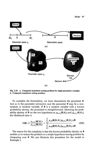
104. 88 2.5 Composite Hypotheses
Example 1 (continued.) We assume that the probability density governing m on H1 is
- oo < M < oo, (297)
Then (296) becomes
f., I ( (R - M)2) I ( M•)
--exp - ·---exp --- dM
- -., Vb a 2a2 vf,;" Om 2om2 ~1
A(R) - I ( R2 ) ffo '7·
-~- exp --2
2
Y 21T a 0
(298)
Integrating and taking the logarithm of both sides, we obtain
R• ~1 2a•(a2 ~ Om2) [in '7 +!In (1 + am•)]·
Ho Om 2 a"
(299)
This result is equivalent to Example 2 on p. 29 because the density used in (297)
makes the two problems identical.
As we expected, the test uses only the magnitude of R because the mean
m has a symmetric probability density.
For the general case given in (296) the actual calculation may be more
involved, but the desired procedure is well defined.
When 8 is a random variable with an unknown density, the best test
procedure is not clearly specified. One possible approach is a minimax
test over the unknown density. An alternate approach is to try several
densities based on any partial knowledge of 8 that is available. In many
cases the test structure will be insensitive to the detailed behavior of the
probability density.
The second case of interest is the case in which 8 is a nonrandom
variable. Here, just as in the problem of estimating nonrandom variables,
we shall try a procedure and investigate the results. A first observation is
that, because 8 has no probability density over which to average, a Bayes
test is not meaningful. Thus we can devote our time to Neyman-Pearson
tests.
We begin our discussion by examining what we call a perfect measure-
ment bound on the test performance. We illustrate this idea for the problem
in Example l.
Example :Z. In this case 8 = M.
From (295)
and (300)
I ( R•)
Ho:Prlm(RIM) = .y21T
0
exp -20 2 •
where M is an unknown nonrandom parameter.

105. Nonrandom Parameters 89
It is clear that whatever test we design can never be better than a hypothetical test
in which the receiver first measures M perfectly (or, alternately, it is told M) and then
designs the optimum likelihood ratio test. Thus we can bound the ROC of any test
by the ROC of this fictitious perfect measurement test. For this example we could use
the ROC's in Fig. 2.9a by letting d2 = M 2 /a2 • Because we are interested in the
behavior versus M, the format in Fig. 2.9b is more useful. This is shown in Fig. 2.26.
Such a curve is called a power function. It is simply a plot of PD for all values of M
(more generally 9) for various values of PF. Because Ha = H1 forM = 0, PD = PF.
The curves in Fig. 2.26 represent a bound on how well any test could do. We now
want to see how close the actual test performance comes to this bound.
The best performance we could achieve would be obtained if an actual test's curves
equaled the bound for all ME X· We call such tests uniformly most powerful (UMP).
In other words, for a given PF a UMP test has a PD greater than or equal to any
other test for all ME X· The conditions for a UMP test to exist can be seen in Fig. 2.27.
t
-4 +4
Mtu-
Fig. 2.26 Power function for perfect measurement test.

106. 90 2.5 Composite Hypotheses
-4 0
M/u~
Fig. 2.27 Power functions for various likelihood ratio tests.
+4
We first construct the perfect measurement bound. We next consider other possible
tests and their performances. Test A is an ordinary likelihood ratio test designed under
the assumption that M = I. The first observation is that the power of this test equals
the bound at M = 1, which follows from the manner in which we constructed the
bound. For other values of M the power of test A may or may not equal the bound.
Similarly, test B is a likelihood ratio test designed under the assumption that M = 2,
and test C is a likelihood ratio test designed under the assumption that M = -I.
In each case their power equals the bound at their design points. (The power functions
in Fig. 2.27 are drawn to emphasize this and are not quantitatively correct away from
the design point. The quantitatively correct curves are shown in Fig. 2.29.) They may
also equal the bound at other points. The conditions for a UMP test are now obvious.
We must be able to design a complete likelihood ratio test (including the threshold)
for every M E x without knowing M.
The analogous result for the general case follows easily.

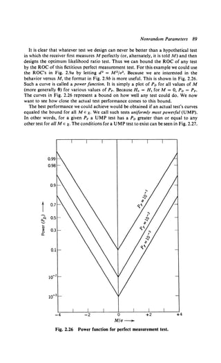
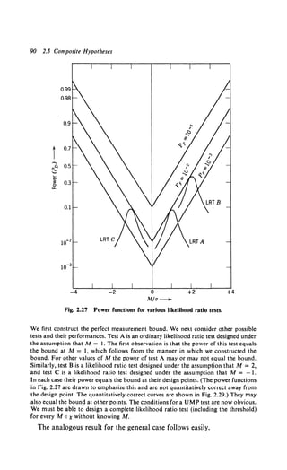
107. Nonrandom Parameters 91
It is clear that in general the bound can be reached for any particular e
simply by designing an ordinary LRT for that particular 9. Now a UMP
test must be as good as any other test for every e. This gives us a necessary
and sufficient condition for its existence.
Property. A UMP test exists ifand only if the likelihood ratio test for every
eE x can be completely defined (including threshold) without knowledge
of e.
The "if" part of the property is obvious. The "only if" follows directly
from our discussion in the preceding paragraph. If there exists some eEX
for which we cannot find the LRT without knowing e, we should have to
use some other test, because we do not know e. This test will necessarily
be inferior for that particular 9 to a LRT test designed for that particular 8
and therefore is not uniformly most powerful.
Returning to our example and using the results in Fig. 2.8, we know that the
likelihood ratio test is
(301)
and
J
., 1 ( R2)
PF = _1- exp - -
2 2 dR,
,+v21Ta a
if M > 0. (302)
(The superscript + emphasizes the test assumes M > 0. The value of y+ may be
negative.) This is shown in Fig. 2.28a.
Similarly, for the case in which M < 0 the likelihood ratio test is
(303)
where
f,- 1 ( R•)
PF = -=- exp -"'2 dR,
-., V21T a 2a
M<O. (304)
This is shown in Fig. 2.28b. We see that the threshold is just the negative of the
threshold forM > 0. This reversal is done to get the largest portion of p,1H,(RJH1)
inside the H, region (and therefore maximize P0 ).
Thus, with respect to Example 1, we draw the following conclusions:
1. If M can take on only nonnegative values (i.e., M0 ~ 0), a UMP test exists
[use (301)].
2. If M can take on only nonpositive values (i.e., M1 ~ 0), a UMP test exists [use
(303)).
3. If M can take on both negative and positive values (i.e., Mo < 0 and M1 > 0),
then a UMP test does not exist. In Fig. 2.29 we show the power function for a likeli-
hood ratio test designed under the assumption that M was positive. For negative
values of M, Po is less than PF because the threshold is on the wrong side.
Whenever a UMP test exists, we use it, and the test works as well as if
we knew e. A more difficult problem is presented when a UMP test does

108. 92 2.5 Composite Hypotheses
0
(b)
'Y+
(a)
M
Fig. 2.28 Effect ofsign ofM: [a] threshold for positive M; [b] threshold for negative M.
not exist. The next step is to discuss other possible tests for the cases in
which a UMP test does not exist. We confine our discussion to one
possible test procedure. Others are contained in various statistics texts
(e.g., Lehmann [17]) but seem to be less appropriate for the physical
problems of interest in the sequel.
The perfect measurement bound suggests that a logical procedure is to
estimate 9 assuming H1 is true, then estimate 9 assuming H 0 is true, and
use these estimates in a likelihood ratio test as if they were correct. If the
maximum likelihood estimates discussed on p. 65 are used, the result is
called a generalized likelihood ratio test. Specifically,
maxp..181 (RI81) H1
Ag{R) = e, ( 19 ;;:: y,
maxp..180 R 0) Ho
8o
(305)
where 91 ranges over all 9 in H1 and 90 ranges over all 9 in H0 • In other
words, we make a ML estimate of 81o assuming that H1 is true. We then
evaluate p..181 (RI91) for 91 = 01 and use this value in the numerator. A
similar procedure gives the denominator.
A simple example of a generalized LRT is obtained by using a slightly
modified version of Example 1.

109. Generalized Likelihood Ratio Test 93
t
-4
Mfu-
Fig. 2.29 Performance of LRT assuming positive M.
Example 2. The basic probabilities are the same as in Example 1. Once again, 8 = M.
Instead of one, we have N independent observations, which we denote by the vector
R. The probability densities are,
N 1 ( (R, - M)2)
Prlm.H1 (RIM,H.) = 0 v'- exp 2 2 •
1-1 27T a a
(306)
N 1 ( R,2 )
Prim,u0 (RIM,Ho) = n .;- exp -p ·
•-tY27Ta a
In this example H. is a composite hypothesis and H 0 , a simple hypothesis. From (198)
(307)

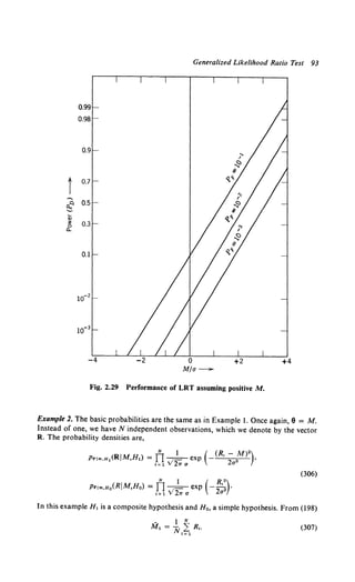
110. 94 2.5 Composite Hypotheses
Then
TI
N 1 { [R,- (1/N) ~J-1 Ri]2
}
V2 exp - 2a• H1
A (R) _ •=1 .,. a >
• - N } < )'.
n -1- exp (- R,2 /2a2 ) Ho
1•1 Y 2w a
(308)
Canceling common terms and taking the logarithm, we have
1 ( N )2H1
In A.(R) = 2 •N L R, ~ In y.
a t= 1 Ho
(309)
The left side of (309) is always greater than or equal to zero. Thus, y can always be
chosen greater than or equal to one. Therefore, an equivalent test is
(
} N )2 H!
N Y. L R, ;:: Y12
t=l Ho
(310)
where Yt ;;:: 0. Equivalently,
II N IH1
lzl Q NY: L R, ~ Y•·
2 , = 1 Ho
(311)
The power function of this test follows easily. The variable z has a variance equal
(a)
(b)
Fig. 2.30 Errors in generalized likelihood ratio test: [a] PF calculation; [b] Po
calculation.

111. Generalized Likelihood Ratio Test 95
to a2 • On H 0 its mean is zero and on H1 its mean is MYN. The densities are sketched
in Fig. 2.30.
and
P, = r:1
v;7T a exp ( -;;) dZ + [ vL a exp (-:a:) dZ
= 2erfc* (;)
PD(M) = s-y1 _/ 1 exp [ (Z- ~VN)"] dZ
-., Y 21T a a
f.. 1 [ (Z- MVN)2]
+ _1- exp - 2 2 dZ
11 v 27T a a
[r + Mv'N] [" - Mv'Nj
=erfc. 1 a + erfc. 1
a - r
Perfect measurement
Generalized LRT
Fig. 2.31 Power function: generalized likelihood ratio tests.
(312)
(313)

112. 96 2.6 The General Gaussian Problem
The resulting power function is plotted in Fig. 2.31. The perfect measure-
ment bound is shown for comparison purposes. As we would expect from
our discussion of ML estimates, the difference approaches zero as
VN Mfa- oo.
Just as there are cases in which the ML estimates give poor results, there
are others in which the generalized likelihood ratio test may give bad
results. In these cases we must look for other test procedures. Fortunately,
in most of the physical problems of interest to us either a UMP test will
exist or a generalized likelihood ratio test will give satisfactory results.
2.6 THE GENERAL GAUSSIAN PROBLEM
All of our discussion up to this point has dealt with arbitrary probability
densities. In the binary detection case PriH1 (RIHl) and PriHo(RIHo) were
not constrained to have any particular form. Similarly, in the estimation
problem Pr1a(RIA) was not constrained. In the classical case, constraints
are not particularly necessary. When we begin our discussion of the wave-
form problem, we shall find that most of our discussions concentrate on
problems in which the conditional density of r is Gaussian. We discuss
this class of problem in detail in this section. The material in this section
and the problems associated with it lay the groundwork for many of the
results in the sequel. We begin by defining a Gaussian random vector and
the general Gaussian problem.
Definition. A set of random variables r1, r2, ••• , rN are defined as jointly
Gaussian if all their linear combinations are Gaussian random variables.
Definition. A vector r is a Gaussian random vector when its components
rh r2, ••• , rN are jointly Gaussian random variables.
In other words, if
N
z = L g1ri f!. GTr (314)
j: 1
is a Gaussian random variable for all finite Gr, then r is a Gaussian vector.
If we define
E(r) = m
and
Cov (r) = E[(r - m)(rr - mT)] f!. A,
then (314) implies that the characteristic function of r is
Mr(jv) f!. E[&vTr] = exp (+jvTm - !vTAv)
(315)
(316)
(317)

113. Likelihood Ratio Test 97
and assuming A is nonsingular the probability density of r is
Pr(R) = [(27T)N12IAIY.J- 1 exp [-t(RT- mT)A- 1(R- m)]. (318)
The proof is straightforward (e.g., Problem 2.6.20).
Definition. A hypothesis testing problem is called a general Gaussian
problem if PrJH,(RIH1) is a Gaussian density on all hypotheses. An
estimation problem is called a general Gaussian problem ifPrJa(RIA) has
a Gaussian density for all A.
We discuss the binary hypothesis testing version ofthe general Gaussian
problem in detail in the text. The M-hypothesis and the estimation
problems are developed in the problems. The basic model for the binary
detection problem is straightforward. We assume that the observation
space is N-dimensional. Points in the space are denoted by the N-dimen-
sional vector (or column matrix) r:
(319)
Under the first hypothesis H1 we assume that r is a Gaussian random
vector, which is completely specified by its mean vector and covariance
matrix. We denote these quantities as
[
E(rliHt)l [m11]
E(r2IH1) 6. m12 6.
E[riHd = : - : - m1.
. .
E(rNIHt) m1N
The covariance matrix is
K1 ~ E[(r - m1)(rT - IDtT)IHd
[
tKll 1K12 1~13
1K21 1K22 ·.
1KN1
We define the inverse of K1 as Q1
Ql ~ K1 1
Q1K1 = K1Q1 =I,
(320)
(321)
(322)
(323)

114. 98 2.6 The General Gaussian Problem
where I is the identity matrix (ones on the diagonal and zeroes elsewhere).
Using (320), (321), (322), and (318), we may write the probability density
ofr on H1,
PriH1 (RJHl) = [(27r)N12 JK1JY.]- 1exp [-1-(RT- m/)Q1(R- m1)]. (324)
Going through a similar set of definitions for H0, we obtain the prob-
ability density
PriHo(RJHo) = [(27T)N12 IKol Y.]- 1exp [--!(RT - moT)Q0(R - mo)]. (325)
Using the definition in (13), the likelihood ratio test follows easily:
JKoJY. exp [-1-(RT- m1T)Q1(R- m1)] ~
IK1JY. exp [-1-(RT - moTIQo(R - mo)] If;, 'YJ·
(326)
Taking logarithms, we obtain
}(RT- m0T) Q0(R- mo) - }(RT- m1T) Q1(R- m1)
H1
~ In 'YJ +tIn IK1I - tIn IKol ~ y*. (327)
Ho
We see that the test consists offinding the difference between two quadratic
forms. The result in (327) is basic to many of our later discussions. For
this reason we treat various cases of the general Gaussian problem in
some detail. We begin with the simplest.
2.6.1 Equal Covariance Matrices
The first special case of interest is the one in which the covariance
matrices on the two hypotheses are equal,
(328)
but the means are different.
Denote the inverse as Q:
(329)
Substituting into (327), multiplying the matrices, canceling common
terms, and using the symmetry of Q, we have
We can simplify this expression by defining a vector corresponding to the
difference in the mean value vectors on the two hypotheses:
(331)

115. Equal Covariance Matrices 99
Then (327) becomes
H1
/(R) ~ amrQR ~ y~
Ho
(332)
or, equivalently,
H1
/(R) ~ RrQ am ~ y~.
Ho
(333)
The quantity on the left is a scalar Gaussian random variable, for it was
obtained by a linear transformation ofjointly Gaussian random variables.
Therefore, as we discussed in Example l on pp. 36-38, we can completely
characterize the performance of the test by the quantity d2• In that
example, we defined d as the distance between the means on the two
hypothesis when the variance was normalized to equal one. An identical
definition is,
d2 t::, [E(/IH1) - E(IIH0)]2•
- Var (/IHo)
Substituting (320) into the definition of/, we have
E(IIH1) = amrQm1
and
(334)
(335)
E(liHo) = amrQm0 . (336)
Using (332), (333), and (336) we have
Var [fiHo] = E{[amrQ(R - mo)][(Rr - mor)Q am]}. (337)
Using (321) to evaluate the expectation and then (323), we have
Var [/IHo] = amrQ am. (338)
Substituting (335), (336), and (338) into (334), we obtain
(339)
Thus the performance for the equal covariance Gaussian case is com-
pletely determined by the quadratic form in (339). We now interpret it for
some cases of interest.
Case 1. Independent Components with Equal Variance. Each r1 has the same
variance o-2 and is statistically independent. Thus
(340)
and
I
Q = 21.
0"
(341)

116. 100 2.6 The General Gaussian Problem
Substituting (341) into (339), we obtain
or
(343)
We see that d corresponds to the distance between the two mean-value
vectors divided by the standard deviation of R1• This is shown in Fig. 2.32.
In (332) we see that
(344)
Thus the sufficient statistic is just the dot (or scalar) product ofthe observed
vector R and the mean difference vector am.
Case 2. Independent Components with Unequal Variances. Here the r1 are
statistically independent but have unequal variances. Thus
(345)
and
a12
0
Q= a22 (346)
0
Substituting into (339) and performing the multiplication, we have
(347)
Now the various difference components contribute to d2 with weighting
that is inversely proportional to the variance along that coordinate. We
can also interpret the result as distance in a new coordinate system.

117. Equal Covariance Matrices 101
Let
.dm'= (348)
and
(349)
This transformation changes the scale on each axis so that the variances
are all equal to one. We see that d corresponds exactly to the difference
vector in this "scaled" coordinate system.
The sufficient statistic is
/(R) = i !l.m;~R;· (350)
t=l at
In the scaled coordinate system it is the dot product of the two vectors
/(R') = .dm'TR'. (351)
Case 3. This is the general case. A satisfactory answer for I and dis already
available in (332) and (339):
/(R) = fl.mTQR
and
Fig. 2.32 Mean-value vectors.
(352)
(353)

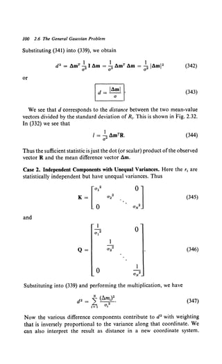
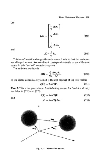
118. 102 2.6 The General Gaussian Problem
Valuable insight into the important features of the problem can be
gained by looking at it in a different manner.
The key to the simplicity in Cases 1 and 2 is the diagonal covariance
matrix. This suggests that we try to represent R in a new coordinate
system in which the components are statistically independent random
variables. In Fig. 2.33a we show the observation in the original coordinate
system. In Fig. 2.33b we show a new set of coordinate axes, which we
denote by the orthogonal unit vectors ~1, ~2, ••• , ~N:
(354)
We denote the observation in the new coordinate system by r'. We want to
choose the orientation of the new system so that the components r; and rj
are uncorrelated (and therefore statistically independent, for they are
Gaussian) for all i =F j. In other words,
E[(r; - m;)(rj - mj)J = ~8~" (355)
where
m; Q E(r;) (356)
and
Var [r;] Q •. (357)
Now the components of r' can be expressed simply in terms of the dot
product of the original vector r and the various unit vectors
(358)
Using (358) in (355), we obtain
E[ci>?Cr - m)(rT - mT)cl>,] = .811. (359)
t;a
(a) (b)
Fig. 2.33 Coordinate systems: [a] original coordinate system; [b] new coordinate
system.

119. Equal Covariance Matrices 103
The expectation of the random part is just K [see (321)]. Therefore (359)
becomes
,1811 = cp1TKcp1. (360)
This will be satisfied if and only if
,1~1 = K~1 for j = 1, 2, ..., N. (361)
To check the "if" part of this result, substitute (361) into (360):
,1811 = cp?,1cpi = ,1811• (362)
where the right equality follows from (354). The "only if" part follows
using a simple proof by contradiction. Now (361) can be written with thej
subscript suppressed:
(363)
We see that the question offinding the proper coordinate system reduces
to the question of whether we can find N solutions to (363) that satisfy
(354).
It is instructive to write (363) out in detail. Each cp is a vector with N
components:
Substituting (364) into (363), we have
Kuq,l + K12q,2 + ···+ K1Nq,N = ,q,l
K2lq,l + K22q,2 + ... + K2Nq,N = ,q,2
KNlq,l + KN2q,2 +... + KNNq,N = "+N
(364)
(365)
We see that (365) corresponds to a set of N homogeneous simultaneous
equations. A nontrivial solution will exist if and only if the determinant
of the coefficient matrix is zero. In other words, if and only if
I I I
Ku - , : K12 : K1a: · · ·
I I I
JK- ,IJ =
--------~----------~----~-
K21 : K22 - , : K2a :
---------~----------; _____1
I I
K31 : Ka2 1
= 0. (366)
'
--------~----------

120. 104 2.6 The General Gaussian Problem
We see that this is an Nth-order polynomial in A. The N roots, denoted by
A
1, A
2, ••• , AN, are called the eigenvalues of the covariance matrix K. It can
be shown that the following properties are true (e.g., [16] or [18]):
1. Because K is symmetric, the eigenvalues are real.
2. Because K is a covariance matrix, the eigenvalues are nonnegative.
(Otherwise we would have random variables with negative variances.)
For each A
1we can find a solution cf>t to (363). Because there is an
arbitrary constant associated with each solution to (363), we may choose
the cl>t to have unit length
(367)
These solutions are called the normalized eigenvectors of K. Two other
properties may also be shown for symmetric matrices.
3. If the roots At are distinct, the corresponding eigenvectors are
orthogonal.
4. If a particular root Ai is of multiplicity M, the M associated eigen-
vectors are linearly independent. They can be chosen to be orthonormal.
We have now described a coordinate system in which the observations
are statistically independent. The mean difference vector can be expressed
as
or in vector notation
am'=
~m~ = cf>1T am
~m~ = cp2T am
cf>NT
The resulting sufficient statistic in the new coordinate system is
N A , R'
/(R') = L~
t= 1 At
and d2 is
(368)
(369)
(370)
(371)

121. Equal Covariance Matrices 105
The derivation leading to (371) has been somewhat involved, but the
result is of fundamental importance, for it demonstrates that there always
exists a coordinate system in which the random variables are uncorrelated
and that the new system is related to the old system by a linear transforma-
tion. To illustrate the technique we consider a simple example.
Example. For simplicity we let N = 2 and m0 = 0. Let
K = e~J
and
To find the eigenvalues we solve
or
Solving,
II ~A 1 ~AI- 0
A1 = I + p,
A
2 = I - p.
To find <!»1 we substitute A1 into (365),
[P
I p] [<fon] = [(I + p
)<fou]
I <fo12 (I + p)<fo12
Solving, we obtain
Normalizing gives
r I ]
+ V2
<1»1 = _1_ •
+ V2
Similarly,
r 1 ]
+ V2
<1»2 = - J2 .
The old and new axes are shown in Fig. 2.34. The transformation is
w ~ ~-~~r~,
[
1 : 1 l
+ V2: V2
I
(372)
(373)
(374)
(375)
(376)
(377)
(378)
(379)
(380)
(381)

122. 106 2.6 The General Gaussian Problem
Rz
R2
t/Jz
Fig. 2.34 Rotation of axes.
, mu - m12
m12 = V2 .
The sufficient statistic is obtained by using (382) in (370),
(382)
l(R') = _1_ (R1 + R2)(m11 + m12) + _1_ (R1 - R.)(mu - m12) (383)
1+p 2 1-p 2
and d2 is
d" = (mu + m12)2 + (mu - m12)2 = (m;l)2 + (m;2 ) 2 •
2(1 + p) 2(1 - p) (1 + p) (1 - p)
(384)
To illustrate a typical application in which the transformation is important we
consider a simple optimization problem. The length of the mean vector is constrained,
(385)
We want to choose m11 and m12 to maximize d2. Because our transformation is a
rotation, it preserves lengths
Looking at (384), we obtain the solution by inspection:
If p > 0, choose m;1 = 0 and m;. = 1.
If p < 0, choose m;l = 1 and m;2 = 0.
If p = 0, all vectors satisfying (385) give the same d2 •
(386)

123. Equal Mean Vectors 107
We see that this corresponds to choosing the mean-value vector to be equal to the
eigenvector with the smallest eigenvalue. This result can be easily extended to N
dimensions.
The result in this example is characteristic ofa wide class ofoptimization
problems in which the solution corresponds to an eigenvector (or the
waveform analog to it).
In this section, we have demonstrated that when the covariance matrices
on the two hypotheses are equal the sufficient statistic /(R) is a Gaussian
random variable obtained by a linear transformation of R. The perform-
ance for any threshold setting is determined by using the value of d2 given
by (339) on the ROC in Fig. 2.9. Because the performance improves
monotonically with increasing d2, we can use any freedom in the param-
eters to maximize d2 without considering the ROC explicitly.
2.6.2 Equal Mean Vectors
In the second special case of interest the mean-value vectors on the two
hypotheses are equal. In other words,
m1 = mo Q m. (387)
Substituting (387) into (327), we have
Hl IK I
!(RT - mT)(Q0 - Q1)(R - m) ~ ln"' + ! ln IK:I = y*. (388)
Because the mean-value vectors contain no information that will tell
us which hypothesis is true, the likelihood test subtracts them from the
received vector. Therefore, without loss of generality, we may assume
that m = 0.
We denote the difference of the inverse matrices as aQ:
aQ ~ Qo - Ql. (389)
The likelihood ratio test may be written as
H1
/(R) Q RT aQR:;:: 2y* Q y'. (390)
Ho
Note that /(R) is the dot product of two Gaussian vectors, RT and aQR.
Thus, /(R) is not a Gaussian random variable.
We now consider the behavior of this test for some interesting special
cases.
Case 1. Diagonal Covariance Matrix on H0 : Equal Variances. Here the
R1 on H0 are statistically independent variables with equal variances:
(391)

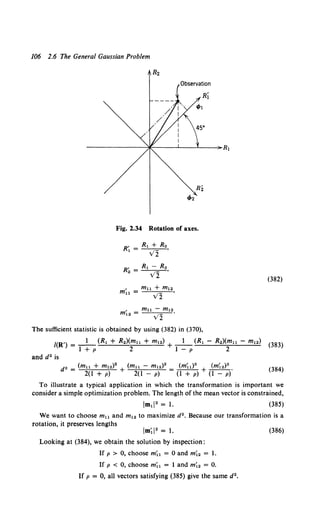
124. 108 2.6 The General Gaussian Problem
We shall see later that (391) corresponds to the physical situation in
which there is "noise" only on H0• The following notation is convenient:
'(392)
On H1 the r1 contain the same variable as on H0 , plus additional signal
components that may be correlated:
(393)
where the matrix K. represents the covariance matrix of the signal com-
ponents. Then
and
1 ( 1 )-1
Q1 = 2 I+ 2K• .
Un Un
It is convenient to write (395) as
1
Q1 = 2 [I- H],
Un
which implies
(394)
(395)
(396)
H = (an21 + KJ- 1Ks = K.(an21 + K.)- 1 = an2Qo- Q1 =an2 dQ. {397)
The H matrix has an important interpretation which we shall develop
later. We take the first expression in (397) as its definition. Substituting
(397) into (389) and the result into (390), we have
(398)
Several subcases are important.
Case lA. Uncorrelated, Identically Distributed Signal Components. In this
case the signal components s1 are independent variables with identical
variances:
(399)
Then
or
(401)

125. Equal Mean Vectors 109
and
1 2 1 2 N
J(R) - - a. RTR = - as "" R 2 {402)
- 2 2 2 2 2+ 2L I•
a,. a,. + a8 a11 a11 a8 I= 1
The constant can be incorporated in the threshold to give
(403)
We now calculate the performance of the test. On both hypotheses /(R)
is the sum of the squares of N Gaussian variables. The difference in the
hypotheses is in the variance of the Gaussian variables. For simplicity, we
shall assume that N is an even integer.
To find p1180(LIH0) we observe that the characteristic function of each
R12 is
(404)
Because of the independence ofthe variables, M1180(jv) can be written as
a product. Therefore
M!IHo(jv) =(I - 2jva,.2)-NI2. (405)
Taking the inverse transform, we obtain p11 80(LI Ho):
L;::: 0,
= 0, L < 0, (406)
which is familiar as the x2 {chi-square) density function with N degrees of
freedom. It is tabulated in several references (e.g., [19] or [3]). For N = 2
it is easy to check that it is the simple exponential on p. 41. Similarly,
L;::: 0,
= 0, L < 0, (407)
where a 1 2 ~ a/ + a 112 •
The expressions for PD and PF are,
PD = r~ [2N12alNr(Nf2)]-lLNI2-le-Li2<T12 dL (408)
and
pF = f"" [2N12a,.Nf(Nj2)]-1LNI2-le-LI2a. 2dL. (409)
Jy•

126. 110 2.6 The General Gaussian Problem
Construction of the ROC requires an evaluation of the two integrals.
We see that for N = 2 we have the same problem as Example 2 on p. 41
and (408) and (409) reduce to
Pn = exp (- 2::2)•
PF = exp ( - 2::2 )•
(410)
and
(411)
For the general case there are several methods of proceeding. First, let
M = N/2 - 1 andy"' = y"J2an2• Then write ·
fY"' XM
PF = 1 - Jo M! e-x dx. (412)
The integral, called the incomplete Gamma function, has been tabulated
by Pearson [21]:
(413)
and
(414)
These tables are most useful for PF ;;:::: w-e and M ::;; 50.
In a second approach we integrate by parts M times. The result is
M ( "')k
PF = exp ( -y"'} L ..r,. (415)
k=O k.
For small PF, y"' is large and we can approximate the series by the last
few terms,
(y"')Me-r- [ M M(M- I} ]
PF = M! 1 + y"' + (y"')2 +... . (416)
Furthermore, we can approximate the bracket as (I - Mjy"') - 1• This
gives
(y"')Me-Y"'
Pp ~ M!(I _ M/y"'f (417)
A similar expression for P0 follows in which y"' is replaced by y1v Q
y"/2a12 • The approximate expression in (417) is useful for manual calcula-
tion. In actual practice, we use (415) and calculate the ROC numerically.
In Fig. 2.35a we have plotted the receiver operating characteristic for some
representative values of Nand a82/an2 •
Two particularly interesting curves are those for N = 8, a/fa/ = 1 and
N = 2, a82/an2 = 4. In both cases the product Na82 fan2 = 8. We see that
when the desired PF is greater than 0.3, P0 is higher if the available "signal
strength" is divided into more components. This suggests that for each PF

127. Equal Mean Vectors 111
and product Na.2/a11
2 there should be an optimum N. In Chapter 4 we
shall see that this problem corresponds to optimum diversity in com-
munication systems and the optimum energy per pulse in radar. In Figs.
2.35b and c we have sketched PM as a function of N for PF = I0-2 and
10-4, respectively, and various Na.2/a11
2 products. We discuss the physical
implications of these results in Chapter 4.
Case lB. Independent Signal Components: Unequal Variances. In this case
the signal components s1 are independent variables with variances a,,2 :
[
a,1
2
K,=
0
(418)
t
0 1.0
Fig. 2.35 a. Receiver operating characteristic: Gaussian variables with identical
means and unequal variances on the two hypotheses.

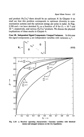
128. 112 2.6 The General Gaussian Problem
Then
and
i
H=
a 2
.,
0
I N a 2 H,
/(R) = -2 L 2 •• 2 Rt2 ~ y'.
an t=l an +a,, Ho
N -
0
Fig. 2.35 b. PM as a function of N [PF = t0- 2 ].
(419)
(420)

129. Equal Mean Vectors 113
The characteristic function of /(R) follows easily, but the calculation of
PF and P0 is difficult. In Section 2.7 we derive approximations to the
performance that lead to simpler expressions.
Case lC. Arbitrary Signal Components. This is, of course, the general case.
We revisit it merely to point out that it can always be reduced to Case IB
by an orthogonal transformation (see discussion on pp. 102-106).
Fig. 2.35 c. PM as a function of N [PF = l0- 4 ].

130. 114 2.6 The General Gaussian Problem
Case 2. Symmetric Hypotheses, Uncorrelated Noise. Case I was unsym-
metric because of the noise-only hypothesis. Here we have the following
hypotheses:
H 1 :r1 = s1 + n1
n;
H0 :r1 = n1
s1 + n,
i =I, ... , N
i = N + 1, ... , 2N,
i = 1, ... , N
i = N + I, ... , 2N,
(421)
where the n1 are independent variables with variance an2 and the s1 have a
covariance matrix K•. Then
(422)
and
(423)
where we have partitioned the 2N x 2N matrices into N x N submatrices.
Then
AQ ~[ ~;~~-·-;~:~-~-i;)-:;]- [(•:~-:-~J---~-.-~~:~l(424)
Using (397), we have
AQ = al2 [~-~--~-]• (425)
n 0: -H
where, as previously defined in (397), H is
H £=. (an21 + K.)- 1K•. (426)
If we partition R into two N x 1 matrices,
R~ [:J (427)
then
(428)
The special cases analogous to IA and IB follow easily.

131. Equal Mean Vectors 115
Case 2A. Uncorrelated, Identically Distributed Signal Components. Let
K, = a,21; (429)
then
(430)
If the hypotheses are equally likely and the criterion is minimum Pr(~).
the threshold TJ in the LRT is unity (see 69). From (388) and (390) we see
that this will result in yv = 0. This case occurs frequently and leads to a
simple error calculation. The test then becomes
N H 1 2N
MR) ~ LR12 ~ L R12 ~ lo(R). (431)
1=1 Ho I=N+l
The probability of error given that H 1 is true is the probability that
/ 0(R) is greater than /1(R). Because the test is symmetric with respect to
the two hypotheses,
Pr (~) = t Pr (~IH1) + t Pr <~IHo) = Pr <~iH1). (432a)
Thus
Pr(£) = f"" dL1P11 1H1 (L1iH1) f"" PloiH1 (LoiHl)dLo. (432b)
Jo JLt
Substituting (406) and (407) in (432b), recalling that N is even, and evalu-
ating the inner integral, we have
Defining
(433)
(434)
This result is due to Pierce [22]. It is a closed-form expression but it is
tedious to use. We delay plotting (434) until Section 2.7, in which we derive
an approximate expression for comparison.
Case lB. Uncorrelated Signal Components: Unequal Variances. Now,
· ..] (435)

132. ll6 2.7 Performance Bounds and Approximations
It follows easily that
As in Case 1B, the performance is difficult to evaluate. The approxi-
mations developed in Section 2.7 are also useful for this case.
2.6.3 Summary
We have discussed in detail the general Gaussian problem and have
found that the sufficient statistic was the difference between two quadratic
forms:
/(R) = !(RT - m0 T)Q0(R - m0) - -!-(RT - m/)Q1(R - m1). (437)
A particularly simple special case was the one in which the covariance
matrices on the two hypotheses were equal. Then
(438)
and the performance was completely characterized by the quantity d2 :
(439)
When the covariance matrices are unequal, the implementation of the
likelihood ratio test is still straightforward but the performance calcula-
tions are difficult (remember that d2 is no longer applicable because /(R) is
not Gaussian). In the simplest case of diagonal covariance matrices with
equal elements, exact error expressions were developed. In the general
case, exact expressions are possible but are too unwieldy to be useful.
This inability to obtain tractable performance expressions is the motivation
for discussion of performance bounds and approximations in the next
section.
Before leaving the general Gaussian problem, we should point out that
similar results can be obtained for the M-hypothesis case and for the
estimation problem. Some of these results are developed in the problems.
2.7 PERFORMANCE BOUNDS AND APPROXIMATIONS
Up to this point we have dealt primarily with problems in which we
could derive the structure of the optimum receiver and obtain relatively
simple expressions for the receiver operating characteristic or the error
probability.
In many cases of interest the optimum test can be derived but an exact
performance calculation is impossible. For these cases we must resort to

133. Derivation 117
bounds on the error probabilities or approximate expressions for these
probabilities. In this section we derive some simple bounds and approxima-
tions which are useful in many problems ofpractical importance. The basic
results, due to Chernoff [28], were extended initially by Shannon [23].
They have been further extended by Fano [24], Shannon, Gallager, and
Berlekamp [25], and Gallager [26] and applied to a problem of interest to
us by Jacobs [27]. Our approach is based on the last two references.
Because the latter part of the development is heuristic in nature, the inter-
ested reader should consult the references given for more careful deriva-
tions. From the standpoint of use in later sections, we shall not use the
results until Chapter 11-3 (the results are also needed for some of the prob-
lems in Chapter 4).
The problem of interest is the general binary hypothesis test outlined in
Section 2.2. From our results in that section we know that it will reduce to
a likelihood ratio test. We begin our discussion at this point.
The likelihood ratio test is
/(R) ~ In A(R) = ln [PriH,(RjH1)] ~ y. (440)
PriHo(RJHo) Ho
The variable /(R) is a random variable whose probability density
depends on which hypothesis is true. In Fig. 2.36 we show a typical
P11H,(LjH1) and PliHo(LJHo).
If the two densities are known, then PF and Pn are given by
Pn = f'P11H,(LjH1)dL,
PF = f"PliHo(LJHo) dL.
(441)
(442)
The difficulty is that it is often hard to find PliH,(LjHi), and even if it
can be found it is cumbersome. Typical of this complexity is Case lA
Fig. 2.36 Typical densities.

134. 118 2.7 Performance Bounds and Approximations
on p. 108, in which there are N Gaussian variables with equal variances
making up the signal. To analyze a given system, the errors may be
evaluated numerically. On the other hand, if we set out to synthesize a
system, it is inefficient (if not impossible) to try successive systems and
evaluate each numerically. Therefore we should like to find some simpler
approximate expressions for the error probabilities.
In this section we derive some simple expressions that we shall use in the
sequel. We first focus our attention on cases in which /(R) is a sum of
independent random variables. This suggests that its characteristic function
may be useful, for it will be the product of the individual characteristic
functions of the R1• Similarly, the moment-generating function will be the
product ofindividual moment-generating functions. Therefore an approxi-
mate expression based on one of these functions should be relatively easy
to evaluate. The first part of our discussion develops bounds on the error
probabilities in terms of the moment-generating function of /(R).
In the second part we consider the case in which /(R) is the sum of a
large number of independent random variables. By the use of the central
limit theorem we improve on the results obtained in the first part of the
discussion.
We begin by deriving a simple upper bound on PF' in terms of the
moment-generating function. The moment-generating function of /(R) on
hypothesis H0 is
where s is a real variable. (The range of s corresponds to those values for
which the integral exists.) We shall see shortly that it is more useful to
write
(444)
so that
p.(s) = ln J~co e•LPIIHo(LIHo) dL. (445)
We may also express p.(s) in terms ofPr1
H 1 (RIH1} and Prl Ho(RIH0). Because
I is just a function of r, we can write (443) as
(446)
Then
(447)

135. Derivation ll9
Using (440),
(448)
or
The function t-L(s) plays a central role in the succeeding discussion. It is
now convenient to rewrite the error expressions in terms of a new random
variable whose mean is in the vicinity of the threshold. The reason for this
step is that we shall use the central limit theorem in the second part of our
derivation. It is most effective near the mean of the random variable of
interest. Consider the simple probability density shown in Fig. 2.37a. To
get the new family of densities shown in Figs. 2.37b-d we multiply px(X) by
e•x for various values ofs (and normalize to obtain a unit area). We see that
for s > 0 the mean is shifted to the right. For the moment we leaves as a
parameter. We see that increasing s "tilts" the density more.
Denoting this new variable as x., we have
Observe that we define x. in terms of its density function, for that is
what we are interested in. Equation 450 is a general definition. For the
density shown in Fig. 2.37, the limits would be (-A, A).
We now find the mean and variance of x,:
(451)
Comparing (451) and (445), we see that
E(x.) = d~~) ~ p.(s). (452)
Similarly, we find
Var (x,) = ji(s). (453)
[Observe that (453) implies that p.(s) is convex.]

136. 120 2.7 Performance Bounds and Approximations
We now rewrite PF in terms of this tilted variable x,:
PF = f"P!IHo(LIHo) dL = f"efl(S)-sXPx.(X) dX
= ell<•> f"e-•Xpx,(X) dX. (454)
We can now find a simple upper bound on PF. For values of s ;::: 0,
-A
-A
-A
-A
for X;::: y.
Pr.(X)
(a)
Pr.0(X)
(b)
(c)
(d)
P",(XJ =p"(X)
when s=O
'Y A
Threshold
so>O
'Y A
'Y A
'Y A
Fig. 2.37 Tilted probability densities.
X
X
(455)

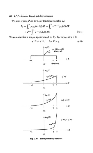
137. Derivation 121
Thus
p < ell<s>-sy foo p (X) dX
F- Xs '
y
s;;:: 0. (456)
Clearly the integral is less than one. Thus
s ~ 0. (457)
To get the best bound we minimize the right-hand side of (457) with
respect to s. Differentiating the exponent and setting the result equal to
zero, we obtain
P,(s) = y.
Because ;l(s) is nonnegative, a solution will exist if
P,(O) ~ y ~ p,(oo).
Because
p,(O) = E(liHo),
(458)
(459)
(460)
the left inequality implies that the threshold must be to the right of the
mean of I on H0 • Assuming that (459) is valid, we have the desired result:
PF ~ exp [p.(s) - sP,(s)], s ;;:: 0, (461)
where s satisfies (458). (We have assumed p.(s) exists for the desired s.)
Equation 461 is commonly referred to as the Chernoff bound [28].
Observe that s is chosen so that the mean of the tilted variable x. is at the
threshold.
The next step is find a bound on PM, the probability of a miss:
(462)
which we want to express in terms of the tilted variable x•.
Using an argument identical to that in (88) through (94), we see that
PliH1 (XIHl) = expiiHo(XIHo). (463)
Substituting (463) into the right side of (450), we have
P11H1 (XIHl) = ell(s)+(l-s)XPx,(X). (464)
Substituting into (462),
PM = ell(S) I~ 00 e<l-s)XPx,(X) dX. (465)
For s::::; 1
for X~ y. (466)
Thus
PM ~ e/l(S)+(l-s)y I~ 00 Px,(X) dX
s ~ I. (467)

138. 122 2.7 Performance Bounds and Approximations
Once again the bound is minimized for
Y = {L(s) (468)
if a solution exists for s :5 I. Observing that
(469)
we see that this requires the threshold to be to the left of the mean of I
on H1 •
Combining (461) and (467), we have
PF :5 exp (p.(s) - s{L(s)]
0 :5 s :5 I (470)
PM :5 exp (p.(s) + (I - s)it(s)]
and
Y = it(s)
is the threshold that lies between the means of I on the two hypotheses.
Confining s to [0, I] is not too restrictive because if the threshold is not
between the means the error probability will be large on one hypothesis
(greater than one half if the median coincides with the mean). If we are
modeling some physical system this would usually correspond to un-
acceptable performance and necessitate a system change.
As pointed out in [25], the exponents have a simple graphical inter-
pretation. A typicalp.(s) is shown in Fig. 2.38. We draw a tangent at the
point at which it(s) = y. This tangent intersects vertical lines at s = 0 and
s = 1. The value of the intercept at s = 0 is the exponent in the PF bound.
The value of the intercept at s = I is the exponent in the PM bound.
S}
,u(st)- s1A (st)
(exponent in PF bound)
,u(st)+ (1-st).U (st)
(exponent in PM bound}
Fig. 2.38 Exponents in bounds.

139. Derivation 123
For the special case in which the hypotheses are equally likely and the
error costs are equal we know that y = 0. Therefore to minimize the bound
we choose that value of s where (L(s) = 0.
The probability of error Pr (t-) is
(471)
Substituting (456) and (467) into (471) and denoting the value s for
which (L(s) = 0 as sm, we have
or
(473)
Up to this point we have considered arbitrary binary hypothesis tests.
The bounds in (470) and (473) are always valid if p.(s) exists. In many cases
ofinterest I(R) consists ofa sum ofa large number ofindependent random
variables, and we can obtain a simple approximate expression for PF and
PM that provides a much closer estimate of their actual value than the
above bounds. The exponent in this expression is the same, but the multi-
plicative factor will often be appreciably smaller than unity.
We start the derivation with the expression for PF given in (454).
Motivated by our result in the bound derivation (458), we choose s so that
Then (454) becomes
This can be written as
(L(s) = 'Y·
PF = e"'<•>J_'x. e-•XPx,(X) dX.
u<•>
PF = e"'(s)-su(s) l"" e+s[Jl(s)-X)Px,(X) dX.
U(S)
(474)
(475)
The term outside is just the bound in (461). We now use a central limit
theorem argument to evaluate the integral. First define a standardized
variable:
6 x, - E(x,) _ x. - (L(s).
Y - (Var [x,])Yz - v'/i(S)
(476)
Substituting (476) into (475), we have
(477)

140. 124 2.7 Performance Bounds and Approximations
In many cases the probability density governing r is such that y ap-
proaches a Gaussian random variable as N (the number of components of
r) approaches infinity.t A simple case in which this is true is the case in
which the r; are independent, identically distributed random variables with
finite means and variances. In such cases, y approaches a zero-mean
Gaussian random variable with unit variance and the integral in (477) can
be evaluated by substituting the limiting density.
f"' e-.Vu(S)r _} e-<Y"I2>dy = e•"i1<•>12 erfc* (svj.i.(s)). (478)
Jo v2"1T
Then
The approximation arises because y is only approximately Gaussian for
finite N. For values of sVj.i.(s) > 3 we can approximate erfc*( ·) by the
upper bound in (71). Using this approximation,
s?. 0. (480)
It is easy to verify that the approximate expression in (480) can also be
obtained by letting
I
py( Y) ~ py(O) ~ • 1_·
v 2"1T
(481)
Looking at Fig. 2.39, we see that this is valid when the exponential
function decreases to a small value while Y « I.
In exactly the same manner we obtain
PM~ {exp [p.(s) +(I- s)P,(s) + (s-; 1}2
iL(s)]}erfc* [(I- s)v}:i(S)].
(482)
For (I - s)Vii(s) > 3, this reduces to
s ~ I. (483)
Observe that the exponents in (480) and (483) are identical to those
obtained by using the Chernoff bound. The central limit theorem argument
has provided a multiplicative factor that will be significant in many of the
applications of interest to us.
t An excellent discussion is contained in Feller [33], pp. 517-520.

141. -s...;;:{;j y
e
Applications 12S
~-----------------------------¥
Fig. 2.39 Behavior of functions.
For the case in which Pr (t") is the criterion and the hypotheses are
equally likely we have
Pr {t) = !PF + !PM
= ! exp [JL(Sm) + s~2
P.(sm)] erfc* [smV;i(sm)]
+ ! exp [JL(Sm) +{l -/m)2
;i{sm)] erfc* [(1 - Sm)VP,{sm)], {484)
where sm is defined in the statement preceding (472) [i.e., p,(sm) = 0 = y].
When both smVj.i(sm) > 3 and {l - Sm)Vj.i(sm) > 3, this reduces to
We now consider several examples to illustrate the application of these
ideas. The first is one in which the exact performance is known. We go

142. 126 2.7 Performance Bounds and Approximations
through the bounds and approximations to illustrate the manipulations
involved.
Example 1. In this example we consider the simple Gaussian problem first introduced
on p. 27:
(486)
and
N 1 ( R ")
PriHo(RIHo) = Il _
1- exp - 2 '2 •
1=1 v 2.,. a a
(487)
Then, using (449)
( ) I J.. J"' IlN 1 [ (R, - m)2s + R,2(1 - s)]dR
p. s = n · · · --=-exp - ,.
_., -"'<=1 v'2.,.a 2a"
(488a)
Because all the integrals are identical,
() = Nl J"' _1_ [-(R- m)2s + R2(1- s)] dR
p. s n _.. v'2.,. a exp 2a" . (488b)
Integrating we have
m2 s(s- 1)d2
p.(s) = Ns(s - 1) 2a 2 Q 2 • (489)
where d2 was defined in the statement after (64). The curve is shown in Fig. 2.40:
!l(s) = (2s - 1)d2
•
2
Using the bounds in (470), we have
( -s2d2 )
PF ::5 exp - 2
-
[ (1 - s)2d2 ]
PM ::5 exp 2
s~
0 ::5 s ::5 I.
Fig. 2.40 JJ.(s) for Gaussian variables with unequal means.
(490)
(491)

143. Applications 127
Because /(R) is the sum of Gaussian random variables, the expressions in (479)
and (482) are exact. Evaluating ji.(s), we obtain
ji.(s) = d 2•
Substituting into (479) and (482), we have
PF = erfc. [sv'ji.(s)] = erfc. (sd)
and
PM = erfc. [(I - s)v';i(s)] = erfc. [(1 - s)d].
These expressions are identical to (64) and (68) (let s = (In TJ)/d2 + t).
(492)
(493)
(494)
An even simpler case is one in which the total probability of error is the criterion.
Then we choose an sm such as p.(sm) = 0. From Fig. 2.40, we see that sm = t. Using
(484) and (485) we have
(495)
where the approximation is very good for d > 6.
This example is a special case of the binary symmetric hypothesis
problem in which p,(s) is symmetric about s = -t. When this is true and the
criterion is minimum Pr (t:), then p,(!) is the important quantity.
The negative of this quantity is frequently referred to as the Bhatta-
charyya distance (e.g., [29]). It is important to note that it is the significant
quantity only when Sm = -t.
In our next example we look at a more interesting case.
Example 2. This example is Case 1A of the general Gaussian problem described on
p. 108:
N 1 ( R,•)
PriH0(RIHo) = n v'- exp -22 ·
1-1 2,. a0 ao
Substituting (497) into (499) gives,
f., I [ sR2 (I - s)R2]
p.(s) = N In v' exp - -
2 2 - 2 2 dR
-., ( 2,. a1 'aA -•) a1 ao
or
A case that will be of interest in the sequel is
al2 = Cln2 + as2,
ao2 = Cln2•
(497)
(498)
(499)
(500)

144. 128 2.7 Performance Bounds and Approximations
Substituting (500) into (499) gives
- = (1 - s) In 1 + __!.._ - In 1 + (l - s) ....!.. •
,.(s) { ( a •) [ a •]}
N/2 a.• a.•
This function is shown in Fig. 2.41.
and
N [ ( a 2
) a"/a 2 ]
p.(s) = 2 -In l + a:• + 1 + (1 '_ ;)a,•fa.•
.. N [ a."fa.• ]2
IL(s) = 2 1 + (1 - s)(a."/a.2 ) •
(501)
(502)
(503)
By substituting (501), (502), and (503) into (479) and (482) we can plot
an approximate receiver operating characteristic. This can be compared
with the exact ROC in Fig. 2.35a to estimate the accuracy of the approxi-
mation. In Fig. 2.42 we show the comparison for N = 4 and 8, and
a//a112 = 1. The lines connect the equal threshold points. We see that the
approximation is good. For larger N the exact and approximate ROC are
identical for all practical purposes.
t-0.3
!J.(S)
N/2
s -
Fig. 2.41 !J.(s) for Gaussian variables with unequal variances.

145. /
0
/
/
/
/
/
/
/
/
/
Equal threshold
lines
/
/
/
/
/
/
/
/
/
/
/
/
/
/
/
/
/
/
Applications 129
/
/
/
/
/
/
/
1.0
Fig. 2.42 Approximate receiver operating characteristics.
Example 3. In this example we consider first the simplified version of the symmetric
hypothesis situation described in Case 2A (p. 115) in which N = 2.
and
where
Then
I ( R.2 + R22 Ra2 + R•2)
Pr1H 1 (R[H.) = (2 )2 2 2 exp - 2 2 - 2 2
~ a1 uo a1 ao
1 ( R1 2 + R2 2 R,O + R4 2)
Prl H 0(R[Ho) = (2 )2 2 2 exp - 2 2 - 2 2 '
7T a1 ao uo 0'1
0'12 = O's2 + f1n2
ao2 = an2·
fL(S) = sIn an2 + (I - s) In (a.2 + a,2) - In (a." + a,"s)
+ (1 - s) In an2 + sIn (an2 + a,O) - In [an2 + a,O(I - s)]
=In (1 +:::)-In [(t + ::·:)(t + (l ~.!)a,O)]·
(504)
(505)
(506)
(507)
The function fL(S) is plotted in Fig. 2.43a. The minimum is at s = t. This is the point
of interest at which minimum Pr (£)is the criterion.

146. 130 2.7 Performance Bounds and Approximations
ll(s)
8 -
Fig. 2.43a fL(s) for the binary symmetric hypothesis problem.
Thus from (473), a bound on the error is,
(1 + a,2fan2)
Pr (£) S t (1 + a,2/2an2)2.
The bound in (508) is plotted in Fig. 2.43b.
Example JA. An interesting extension of Example 3 is the problem in which
0
K,=
0
(508)
(509)

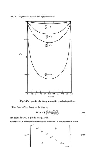
147. Applications 131
o.sr-----
t 0.01
Pr(E)
Fig. 2.43b Bound on the probability of error (Pr(e)).
The r.'s are independent variables and their variances are pairwise equal. This is a
special version of Case 2B on p. ll5. We shall find later that it corresponds to a
physical problem of appreciable interest.
Because of the independence, l'(s) is just the sum of the p.(s) for each pair, but each
pair corresponds to the problem in Example 3. Therefore
N/2 ( a 2) N/2 {( a 2) ( a 2)}
#'(s) = L In 1 +-; - L In 1 +s-; 1 +(1 - s)-; ·
t=l O'n t=l Un O'n
(510)
Then
. N/2 [ a,,2 a,,2 ]
p.(s) = - L 2 2 - 2 2
l=l an + sa,, an + (1 - s)a,1
(511)
and
(512)
For a minimum probability of error criterion it is obvious from (511) that sm = t.
Using (485), we have
Pr (~) ~ [wNi ( 2 a,,; 2)2] -y. exp [~In (1 +a,,:} - 2~In (1 +2
a,,:)] (513)
i=l 0 n + 0 s1 t=l 0 n t=l 0 n
or
Pr <~> ~ (514)

148. 132 2.7 Performance Bounds and Approximations
For the special case in which the variances are equal
a,.2 = a,2 (SIS)
and (514) reduces to
(Sl6)
Alternately, we can use the approximation given by (484). For this case it reduces to
Pr (£) ~ [0
1++a~;;~:::)•r•exp [~(1 :·:~~f;a.•rl erfc. [ (;rc:·:~~f;a.•)l
(SI7)
In Fig. 2.44 we have plotted the approximate Pr (•) using (Sl7) and exact Pr (£)
which was given by (434). We see that the approximation is excellent.
The principal results of this section were the bounds on PF and PM
given in (470) and (473) and the approximate error expressions given in
(479), (480), (482), (483), (484), and (485). These expressions will enable us
to find performance results for a number of cases of physical interest.
--Exact
- - Approx
t
Pr(E)
0.01
100
Fig. 2.44 Exact and approximate error expressions for the binary symmetric hypothesis
case.

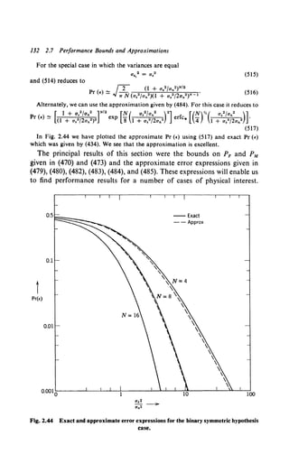
149. 2.8 Summary 133
Results for some other cases are given in Yudkin [34] and Goblick [35]
and the problems. In Chapter 11-3 we shall study the detection of Gaussian
signals in Gaussian noise. Suitable extensions of the above bounds and
approximations will be used to evaluate the performance of the optimum
processors.
2.8 SUMMARY
In this chapter we have derived the essential detection and estimation
theory results that provide the basis for our work in the remainder of the
book.
We began our discussion by considering the simple binary hypothesis
testing problem. Using either a Bayes or a Neyman-Pearson criterion, we
were led to a likelihood ratio test, whose performance was described by a
receiver operating characteristic. Similarly, the M-hypothesis problem led
to the construction of a set of likelihood ratios. This criterion-invariant
reduction of the observation to a single number in the binary case or to
M - I numbers in the M hypothesis case is the key to our ability to solve
the detection problem when the observation is a waveform.
The development of the necessary estimation theory results followed a
parallel path. Here, the fundamental quantity was a likelihood function.
As we pointed out in Section 2.4, its construction is closely related to the
construction of the likelihood ratio, a similarity that will enable us to
solve many parallel problems by inspection. The composite hypothesis
testing problem showed further how the two problems were related.
Our discussion through Section 2.5 was deliberately kept at a general
level and for that reason forms a broad background of results applicable
to many areas in addition to those emphasized in the remainder of the
book. In Section 2.6 we directed our attention to the general Gaussian
problem, a restriction that enabled us to obtain more specific results than
were available in the general case. The waveform analog to this general
Gaussian problem plays the central role in most of the succeeding work.
The results in the general Gaussian problem illustrated that although we
can always find the optimum processor the exact performance may be
difficult to calculate. This difficulty motivated our discussion of error
bounds and approximations in Section 2.7. These approximations will lead
us to useful results in several problem areas of practical importance.
2.9 PROBLEMS
The problems are divided into sections corresponding to the major
sections in the chapter. For example, section P2.2 pertains to text material

150. 134 2.9 Problems
in Section 2.2. In sections in which it is appropriate the problems are
divided into topical groups.
As pointed out in the Preface, solutions to individual problems are
available on request.
P2.2 Binary Hypothesis Tests
SIMPLE BINARY TESTS
Problem 2.2.1. Consider the following binary hypothesis testing problem:
H1:r = s + n,
H 0 :r = n,
where s and n are independent random variables.
p,(S) = ae-as
0
Pn(N) = be-"N
0
s ~ 0,
s < 0,
N<::: 0,
N < 0.
I. Prove that the likelihood ratio test reduces to
H1
R ~ i'·
Ho
2. Find y for the optimum Bayes test as a function of the costs and a priori
probabilities.
3. Now assume that we need a Neyman-Pearson test. Find y as a function of PF,
where
PF ~ Pr(say H1IHo is true).
Problem 2.2.2. The two hypotheses are
I
H1 :p,(R) = 2exp (-IRI)
H0 :p,(R) = ) 2.. exp ( -~ R2)
l. Find the likelihood ratio A(R).
2. The test is
H1
A(R) ~ "'I·
Ho
Compute the decision regions for various values of "'I·
Problem 2.2.3. The random variable x is N(O, a). It is passed through one of two
nonlinear transformations.
Find the LRT.
H1:y = x2 ,
Ho:y = x3 •
Problem 2.2.4. The random variable x is N(m, a). It is passed through one of two
nonlinear transformations.
Find the LRT.
H1:y = e",
Ho:y = x2 •

151. Binary Hypothesis Tests 135
Problem 2.2.5. Consider the following hypothesis-testing problem. There are K
independent observations.
H1 : r, is Gaussian, N(O, a1),
H 0 :r, is Gaussian, N(O, a 0 ),
where a0 < a1 •
I. Compute the likelihood ratio.
2. Assume that the threshold is '7:
H1
A(R) :i; "'·
Ho
i =I, 2, ..., K,
i= 1,2, ... ,K,
Show that a sufficient statistic is /(R) = ~~= 1 R,2• Compute the threshold y for the test
in terms of.,, a0 , a 1 •
3. Define
H1
/(R) :i; y
Ho
PF = Pr (choose Hd Ho is true),
PM = Pr (choose Hoi H, is true).
Find an expression for PF and PM.
4. Plot the ROC forK= I, a 12 = 2, a 0 2 = I.
5. What is the threshold for the minimax criterion when eM = CF and Coo = Cu = 0?
Problem 2.2.6. The observation r is defined in the following manner:
r = bm1 + n:H,
r = n :Ho,
where band n are independent zero-mean Gaussian variables with variances ab2 and
a.2, respectively
I. Find the LRT and draw a block diagram of the optimum processor.
2. Draw the ROC.
3. Assume that the two hypotheses are equally likely. Use the criterion of minimum
probability of error. What is the Pr(•)?
Problem 2.2.7. One of two possible sources supplies the inputs to the simple communi-
cation channel as shown in the figure.
Both sources put out either I or 0. The numbers on the line are the channel
transition probabilities; that is,
Pr(a out II in) = 0.7.
The source characteristics are
Source
Source I: Pr(l) = 0.5, Pr(O) = 0.5;
Source 2: Pr(l) = 0.6, Pr(O) = 0.4.
1 or 0
0.6
Channel

152. 136 2.9 Problems
To put the problem in familiar notation, define
(a) false alarm-say source 2 when source l is present;
(b) detection-say source 2 when source 2 is present.
l. Compute the ROC of a test that maximizes Po subject to the constraint that
PF =a.
2. Describe the test procedure in detail for a = 0.25.
Problem 2.2.8. The probability densities on the two hypotheses are
l
PxJH,(XiH,) = 1r[l + (X_ a,)•]
where ao = 0 and a, = l.
I. Find the LRT.
2. Plot the ROC.
-oo <X< oo:H,
Problem 2.2.9. Consider a simple coin tossing problem:
H,: heads are up, Pr [H,] £ P,
Ho: tails are up, Pr [Hal£ Po < P,.
i = 0, I.
N independent tosses of the coin are made. Show that the number of observed heads,
NH, is a sufficient statistic for making a decision between the two hypotheses.
Problem2.2.10. A sample function ofa simple Poisson counting process N(t) is observed
over the interval T:
hypothesis H1 : the mean rate is k,: Pr (H1) = t.
hypothesis Ho: the mean rate is ko: Pr (Ho) = t.
I. Prove that the number of events in the interval Tis a "sufficient statistic" to
choose hypothesis Ho or H,.
2. Assuming equal costs for the possible errors, derive the appropriate likelihood
ratio test and the threshold.
3. Find an expression for the probability of error.
Problem 2.2.11. Let
where the X; are statistically independent random variables with a Gaussian density
N(O, a). The number of variables in the sum is a random variable with a Poisson
distribution:
)lk
Pr(n = k) = k!e-' k = 0, 1, ....
We want to decide between the two hypotheses,
H,:n 5 I,
Ho: n > I.
Write an expression for the LRT.
Problem 2.2.12. Randomized tests. Our basic model of the decision problem in the
text (p. 24) did not permit randomized decision rules. We can incorporate them by
assuming that at each point R in Z we say H, with probability tf>(R) and say H0 with
probability l - t/>(R). The model in the text is equivalent to setting ,P(R) = I for all
R in z, and ,P(R) = 0 for all R in Z0 •
I. We consider the Bayes criterion first. Write the risk for the above decision model.
2. Prove that a LRT minimizes the risk and a randomized test is never necessary.

153. Binary Hypothesis Tests 137
3. Prove that the risk is constant over the interior of any straight-line segment on
an ROC. Because straight-line segments are generated by randomized tests, this is an
alternate proof of the result in Part 2.
4. Consider the Neyman-Pearson criterion. Prove that the optimum test always
consists of either
(i) an ordinary LRT with PF = a or
(ii) a probabilistic mixture of two ordinary likelihood ratio tests constructed as
H1 H1
follows: Test 1: A(R) ~ 'l gives PF = a+. Test 2: A(R) > 'l gives PF = a-, where
[a-, a+] is the smallest interval containing a. cf>(R) is 0 or 1 except for those R where
cf>(R) = 'l· (Find cf>(R) for this set.)
MATHEMATICAL PROPERTIES
Problem 2.2.13. The random variable A(R) is defined by (13) and has a different
probability density on H1 and Ho. Prove the following:
1. £(A"IH1) = E(An+ 11Ho),
2. E(AIHo) = I,
3. £(AIH1) - E(AIHo) = Var (AIH0).
Problem 2.2.14. Consider the random variable A. In (94) we showed that
Pt.IH1(XIH1) = XPt.IHo(XIHo).
1. Verify this relation by direct calculation ofp,..1H1(·) andp,.. IHo<·)for the densities
in Example I (p. 27, (19) and (20)].
2. On page 37 we saw that the performance of the test in Example 1 was completely
characterized by d2 • Show that
d 2 = In [1 + Var (AIHo)].
Problem 2.2.15. The function erfc. (X) is defined in (66):
1. Integrate by parts to establish the bound
1 ( 1 ) ( x•) 1 ( x•)
v'21r X 1 - x• exp - 2 < erfc. (X)< V21T Xexp - 2 ,
2. Generalize part 1 to obtain the asymptotic series
X> 0.
erfc. (X)= .t 1 e-x•,•[1 + "f(-l)m 1·3· )?mm-1) + R.]·
v21TX m=l
The remainder is less than the magnitude of the n + 1 term and is the same sign.
Hint. Show that the remainder is
R = [<-1)•+ 1 1·3· · ·(2n- 1)] 8
n x••+2 ,
where
f"' ( 2t)-·-··
8 = Jo e-• 1 +_i2 ' dt < 1.
3. Assume that X = 3. Calculate a simple bound on the percentage error when
erfc.(3) is approximated by the first n terms in the asymptotic series. Evaluate this
percentage error for n = 2, 3, 4 and compare the results. Repeat for X = 5.

154. JJ8 2.9 Problems
Problem 2.2.16.
1. Prove
Hint. Show
1 ( X")
erfc. (X) < 2. exp - 2 , X> 0.
[erfc. (X)]2 = Pr(x <:!:: X, y <:!:: X) < Pr(x2 + y2 <:!:: 2X2),
where x and y are independent zero-mean Gaussian variables with unit variance.
2. For what values of X is this bound better than (71)?
HIGHER DIMENSIONAL DECISION REGIONS
A simple binary test can always be reduced to a one-dimensional decision region.
In many cases the results are easier to interpret in two or three dimensions. Some
typical examples are illustrated in this section.
Problem 2.2.17.
H,:p,.,,,.2 1H1(X,,X.IH,) = -
4
1 [exp (- 2
x•:- 2
x•:) + exp (- 2
x•:- 2
x•:)]·
7Ta1a0 a1 a0 a0 a1
- CX) < x,x. < CX).
1 ( x,• x.•)
Ha:p,.1 ,x2 1Ho(X, X.IHo) = -
2 2 exp - -
2 2 - -
2 2 •
wao ao ao
-CX) < x,x. < CXl,
1. Find the LRT.
2. Write an exact expression for Po and PF. Upper and lower bound Po and PF
by modifying the region of integration in the exact expression.
Problem 2.2.18. The joint probability density of the random variables x, (i =
1, 2, .. , M) on H, and Ho is
where
PxiH0(XIHo) = Il _
1
1 exp (- 2
x':)
lal V27Ta a
-CX) < x, < CX),
1. Find the LRT.
2. Draw the decision regions for various values of 'I in the X, X2-plane for the
special case in which M = 2 and p, = P• = t.
3. Find an upper and lower bound to PF and P0 by modifying the regions of
integration.
Problem 2.2.19. The probability density of r, on the two hypotheses is
The observations are independent.
i = 1, 2, ... , N,
k = 0, 1.
1. Find the LRT. Express the test in terms of the following quantities:
N
Ia = L Rh
1=1

155. M-Hypothesis Tests 139
2. Draw the decision regions in the la,l~-plane for the case in which
2mo = m1 > 0,
Problem 2.2.20 (continuation).
1. Consider the special case
2al = ao.
mo =0,
a0 =a1.
Draw the decision regions and compute the ROC.
2. Consider the special case
Draw the decision regions.
mo = m1 = 0,
a12 = a,2 + a,.2,
Problem 2.2.21. A shell is fired at one of two targets: under H1 the point of aim has
coordinates Xt, Y1o z1; under H0 it has coordinates Xo, Yo, z0. The distance of the
actual landing point from the point of aim is a zero-mean Gaussian variable, N(O, a},
in each coordinate. The variables are independent. We wish to observe the point of
impact and guess which hypothesis is true.
1. Formulate this as a hypothesis-testing problem and compute the likelihood
ratio. What is the simplest sufficient statistic? Is the ROC in Fig. 2.9a applicable?
If so, what value of d 2 do we use?
2. Now include the effect of time. Under H" the desired explosion time is '"
(k = 1, 2). The distribution of the actual explosion time is
1 ( (T - /1<)2)
P•IH"(T} = _1 - exp - 2 2 •
v 27T a1 a,
Find the LRT and compute the ROC.
P2.3 M-Hypothesis Tests
Problem 2.3.1.
-<X) < T < <X>,
k = 1, 2.
1. Verify that the M-hypothesis Bayes test always leads to a decision space whose
dimension is less than or equal to M - 1.
2. Assume that the coordinates of the decision space are
A (R) t::. PriH"(RIH")
" - PriH0 (RIHo)'
k = 1, 2, ... , M- 1.
Verify that the decision boundaries are hyperplanes.
Problem 2.3.2. The formulation of the M-hypothesis problem in the text leads to an
efficient decision space but loses some of the symmetry.
1. Starting with (98) prove that an equivalent form of the Bayes test is the
following:
Compute
M•l
fJ, !l L c,l Pr (H1IR}, i = 0, 1, ..., M- 1,
1=0
and choose the smallest.

156. 140 2.9 Problems
2. Consider the special cost assignment
Cu = 0,
c,1 = c,
i = 0, 1, 2, ... , M- 1,
i"¢j,i,j=0,1,2, ...,M-l.
Show that an equivalent test is the following:
Compute
Pr (H,IR), i = 0, 1, 2, ... , M - 1,
and choose the largest.
Problem 2.3.3. The observed random variable is Gaussian on each of five hypotheses.
where
m1 = -2m,
mo = -m,
ma = 0,
m4 = m,
ms =2m.
-oo < R < oo;
k = 1,2, ...,5,
The hypotheses are equally likely and the criterion is minimum Pr (f).
1. Draw the decision regions on the R-axis.
2. Compute the error probability.
Problem 2.3.4. The observed random variable r has a Gaussian density on the three
hypotheses,
1 [ (R - m~c)2 ]
PriH~c(RIH~c) = . 1 - exp - 2 2 •
v 27T a1c a~c
-oo<R<oo
k = 1, 2, 3,
where the parameter values on the three hypotheses are,
H1:m1 = 0, a1 = aa,
H2:m2 = m, a2 = aa,
Ha:ma = 0, a3 = a6,
(m > 0),
(a6 > aa).
The three hypotheses are equally likely and the criterion is minimum Pr (•).
1. Find the optimum Bayes test.
2. Draw the decision regions on the R-axis for the special case,
ap2 = 2aa2,
fla = m.
3. Compute the Pr (f) for this special case.
Problem 2.3.5. The probability density of r on the three hypotheses is
a112 = a212 = Un2,
a122 = Us2 + O'n 2,
a132 = an2,
a222 = Un2 ,
aoa2 = a,2 + an2 •
-oo < R1 , R2 < oo,
k = 1, 2, 3,

157. Estimation 141
The cost matrix is
where 0 :5 a < 1 and Pr (H.) = Pr (H") §. p. Define h = R12 and /2 = R22 •
1. Find the optimum test and indicate the decision regions in the h, I.-plane.
2. Write an expression for the error probabilities. (Do not evaluate the integrals.)
3. Verify that for a= 0 this problem reduces to 2.2.17.
Problem 2.3.6. On H" the observation is a value of a Poisson random variable
k n
Pr (r = n) = nm! e-"m, m = 1, 2, ... , M,
where km = mk. The hypotheses are equally likely and the criterion is minimum Pr (€).
l. Find the optimum test.
2. Find a simple expression for the boundaries of the decision regions and indicate
how you would compute the Pr (•).
Problem 2.3.7. Assume that the received vector on each of the three hypotheses is
Ho: r = mo + n,
H.: r = m. + n,
H.: r = m2 + n,
where
r Q [::] , m, Q [:::] , n Q [::].
r" m,3 n3
The m, are known vectors, and the components of n are statistically independent,
zero-mean Gaussian random variables with variance a 2 •
I. Using the results in the text, express the Bayes test in terms of two sufficient
statistics.
Find explicit expressions for c, and d,. Is the solution unique?
2. Sketch the decision regions in the h, /2-plane for the particular cost assignment,
P2.4 Estimation
Problem 2.4.1. Let
where a, b, and
Ua2 , Ub2 , and Un 2 •
Coo = Cu = C22 = 0,
C12 = C21 = Cot = Cto = -!Co2 = -!C2o > 0.
BAYES ESTIMATION
r = ab + n,
independent zero-mean Gaussian variables with variances
I. What is dmap?
2. Is this equivalent to simultaneously finding dmap, bmap?

158. 142 2.9 Problems
3. Now consider the case in which
where the b, are independent zero-mean Gaussian variables with variances ab,2•
(a) What is dmap?
(b) Is this equivalent to simultaneously finding dmap, b1,map?
(c) Explain intuitively why the answers to part 2 and part 3b are different.
Problem 2.4.2. The observed random variable is x. We want to estimate the parameter
.. The probability density of x as a function of , is,
PxiA(XI.) = .e-Ax,
= 0,
X~0,.>0,
X< 0.
The a priori density of. depends on two parameters: n., 1
•.
, ~ 0,
, < 0.
1. Find £(.) and Var (.) before any observations are made.
2. Assume that one observation is made. FindpA1x(.IX). What interesting property
does this density possess? Find Ama and E[(1ms- .)2].
3. Now assume that n independent observations are made. Denote these n ob-
servations by the vector x. Verify that
where
and
Find Am. and E[(Am• - .)2 ).
4. Does Amap = Am•?
I'= I+ 1
••
n' = n + "••
R
I= L x,.
I= 1
, ~ 0,
, < 0,
Comment. ReprodiiCing Densities. The reason that the preceding problem was
simple was that the a priori and a posteriori densities had the same functional form.
(Only the parameters changed.) In general,
(AIR) _ Prla(RIA)p.(A)
Pair - p,(R) '
and we say that pa(A) is a reproducing density or a conjugate prior density [with respect
to the transition density p,1.(RIA)] if the a posteriori density is of the same form as
p.(A). Because the choice of the a priori density is frequently somewhat arbitrary, it is
convenient to choose a reproducing density in many cases. The next two problems
illustrate other reproducing densities of interest.

159. Estimation 143
Problem 2.4.3. Let
r=a+n,
where n is N(O, an). Then
1 [ (R- A)"]·
Prio(RIA) = .;- exp
v 21T an 2an2
l. Verify that a conjugate priori density for a is N(m0, ;:) by showing that
where
Poir(AIR) = N(m1, a1),
and
u2
a2- __
n_,
1 - 1 + ko2
2. Extend this result to N independent observations by verifying that
where
Polr(AIR) = N(mN, aN),
and
Observe that the a priori parameter k02 can be interpreted as an equivalent number of
observations (fractional observations are allowed).
Problem 2.4.4. Consider the observation process
A~2 [ A ]
Prio(RIA) = (21r)Yz exp -2 (R - m)2 •
where m is known and A is the parameter of interest (it is the reciprocal of the variance).
We assume that N independent observations are available.
l. Verify that
k1
p.(Alk~o k.) = c(A 2- 1) exp (-tAk1k2), A ;;:: 0,
k~o k. > 0,
(c is a normalizing factor) is a conjugate prior density by showing that
Poir(AIR) =p.(Alk~. k~).
where
k~ = ~ (k1k• + Nw),
k!. =k1 + N,
1 N
w = N 2: (R1 - m)2•
1•1
Note that k~o k2 are simply the parameters in the a priori density which are chosen
based on our a priori knowledge.
2. Find t2ma•

160. 144 2.9 Problems
Problem 2.4.5. We make K observations: R" .. ., Rx, where
r, =a+ n,.
The random variable a has a Gaussian density N(O, aa). The n1 are independent
Gaussian variables N(O, an).
1. Find the MMSE estimate dms·
2. Find the MAP estimate dmap·
3. Compute the mean-square error.
4. Consider an alternate procedure using the same r1•
(a) Estimate a after each observation using a MMSE criterion.
This gives a sequence of estimates a,(R,), a.(R" R2) •.• atCR".. .. R1) •••
dx(R" .. ., Rx). Denote the corresponding variances as a,2 , a,O, ... , ax2 •
(b) Express d1 as a function of d1 _" af_, and R1•
(c) Show that
l - l j
---+-·
a? O'a2 O'n2
Problem 2.4.6. [36]. In this problem we outline the proof of Property 2 on p. 61. The
assumptions are the following:
(a) The cost function is a symmetric, nondecreasing function. Thus
C(X) = C(-X)
C(X,) ;::: C(X.) for X1 ;::: X2 ;::: 0, (P.l)
which implies
dC(X) 0 f X
dX;::; or 2::0. (P.2)
(b) The a posteriori probability density is symmetric about its conditional mean
and is nonincreasing.
(c) lim C(X)Pxlr(XIR) = 0.
x~"'
(P.3)
We use the same notation as in Property 1 on p. 61. Verify the following steps:
1. The conditional risk using the estimate ais
(P.4)
2. The difference in conditional risks is
Ll.'lt = .'lt(aiR) - .'lt(l'imsiR) = rC(Z)[p,lr(Z + d - dmsiR)p,lr(Z - a+ l'imsiR)
- 2Pzlr(ZIR)] dZ. (P.5)
3. For a > dms the integral of the terms in the bracket with respect to Z from 0 to
Z 0 is
r-•ms[Pzlr(Zo + YIR)- Pzlr(Zo- YIR)] dY Q g(Zo) (P.6)
4. Integrate (P.5) by parts to obtain
Ll.'lt = C(Z)g(Z) 1
: - rd~i) g(Z) dZ, (P.7)
5. Show that the assumptions imply that the first term is zero and the second term
is nonnegative.
6. Repeat Steps 3 to 5 with appropriate modifications for ti < dms·

161. Estimation 145
7. Observe that these steps prove that dms minimizes the Bayes risk under the above
assumptions. Under what conditions will the Bayes estimate be unique?
NONRANDOM PARAMETER ESTIMATION
Problem 2.4.7. We make n statistically independent observations: rt. r2, ••. , rno with
mean m and variance u2 • Define the sample variance as
V = ! i (R1 - i ~)2
•
nl=l <=1 n
Is it an unbiased estimator of the actual variance?
Problem 2.4.8. We want to estimate a in a binomial distribution by using n observa-
tions.
Pr (r eventsla) = (:)a•(I - a)•-•, r = 0, I, 2, ... , n.
1. Find the ML estimate of a and compute its variance.
2. Is it efficient?
Problem 2.4.9.
I. Does an efficient estimate of the standard deviation u of a zero-mean Gaussian
density exist?
2. Does an efficient estimate of the variance a" of a zero-mean Gaussian density
exist?
Problem 2.4.10 (continuation). The results of Problem 2.4.9 suggest the general
question. Consider the problem of estimating some function of the parameter A, say,
f,(A). The observed quantity is Rand p,1.(RIA) is known. Assume that A is a nonran-
dom variable.
1. What are the conditions for an efficient estimate /t(A) to exist?
2. What is the lower bound on the variance of the error of any unbiased estimate
off,(A)?
3. Assume that an efficient estimate off 1(A) exists. When can an efficient estimate
of some other function [ 2(A) exist?
Problem 2.4.11. The probability density of r, given A, and A2 is:
Pria1.a2 (RIA, A.)= (21TA2)-Yz exp [ (R ;A:1)
2
];
that is, A, is the mean and A. is the variance.
1. Find the joint ML estimates of A1 and A. by using n independent observations.
2. Are they biased?
3. Are they coupled?
4. Find the error covariance matrix.
Problem 2.4.12. We want to transmit two parameters, A, and A2 • In a simple attempt
to achieve a secure communication system we construct two signals to be transmitted
over separate channels.
s1 = xuA1 + x12A2,
s2 = x21A1 + X22A2,
where x,~o i, j = I, 2, are known. The received variables are
r, = s, + n,
r2 = s2 + n2.

162. 146 2.9 Problems
The additive noises are independent, identically distributed, zero-mean Gaussian
random variables, N(O, un). The parameters At and A2 are nonrandom.
1. Are the ML estimates d1 and d2 unbiased?
2. Compute the variance of the ML estimates ch and d••
3. Are the ML estimates efficient? In other words, do they satisfy the Cramer-Rao
bound with equality?
Problem 2.4.13. Let
N
y = L X~o
i=l
where the x, are independent, zero-mean Gaussian random variables with variance
u,.2• We observe y. In parts 1 through 4 treat Nasa continuous variable.
1. Find the maximum likelihood estimate of N.
2. Is iim, unbiased?
3. What is the variance of iim1?
4. Is iim, efficient?
5. Discuss qualitatively how you would modify part 1 to take into account that N
is discrete.
Problem 2.4.14. We observe a value of the discrete random variable x.
A'
Pr(x = iiA) = ""'ie-A, i = 0, 1,2, ... ,
I.
where A is nonrandom.
1. What is the lower bound on the variance of any unbiased estimate, d(x)?
2. Assuming n independent observations, find an d(x) that is efficient.
Problem 2.4.15. Consider the Cauchy distribution
p,. 1a(XiA) = {w[l + (X- A)2 ]}- 1 •
Assume that we make n independent observations in order to estimate A.
1. Use the Cramer-Rao inequality to show that the variance of any unbiased
estimate of A has a variance greater than 2/n.
2. Is the sample mean a consistent estimate?
3. We can show that the sample median is asymptotically normal, N(A, w/V4n).
(See pp. 367-369 of Cramer [9].) What is the asymptotic efficiency of the sample
median as an estimator?
Problem 2.4.16. Assume that
1 { (R12 - 2pR1R• + R2")}
Prt·'•lp(R., R•iP) = 2w(l - p•)Y. exp - 2(1 - p•) .
We want to estimate the correlation coefficient p by using n independent observa-
tions of (R., R2).
1. Find the equation for the ML estimate p.
2. Find a lower bound on the variance of any unbiased estimate of p.
MATHEMATICAL PROPERTIES
Problem 2.4.17. Consider the biased estimate d(R) of the nonrandom parameter A.
E(d(R)) = A + B(A).

163. Estimation 147
Show that
(1 + dB(A)/dA)0
var [d(R)] ~ E{[alnp~~<RIA>r}"
This is the Cramer-Rao inequality for biased estimates. Note that it is a bound on the
mean-square error.
Problem 2.4.18. Let pr1a(RJA) be the probability density of r, given A. Let h be an
arbitrary random variable that is independent of r defined so that A + h ranges over
all possible values of A. Assume that ph1(H) and PhiH) are two arbitrary probability
densities for h. Assuming that d(R) is unbiased, we have
f[d(R) - (A + H)]Prla(RJA + H) dR = 0.
Multiplying by ph1(H) and integrating over H, we have
fdH Ph1(H) f[d(R) - (A + H)]Prla(RJA + H) dR = 0.
1. Show that
Var [d(R) - A] ~ [El(h) - E2(h)]2 2
f((JPrla(RJA + H)[ph1(H)- Ph2(H)] dH) )dR
Prla(RJA)
for any Ph1 (H) and Ph2 (H). Observe that because this is true for all Ph1 (H) and Ph2 (H),
we may write
Var [d(R) - A] ~ sup (right-hand side of above equation).
Pnl,Ph2
Comment. Observe that this bound does not require any regularity conditions.
Barankin [15] has shown that this is the greatest lower bound.
Problem 2.4.19 (continuation). We now derive two special cases.
1. First, let Ph2 (H) = o(H). What is the resulting bound?
2. Second, let Ph1 (H) = o(H - Ho), where Ho =F 0. Show that
Var [a(R)- A]~ (inc{_!, [Jpi,a(RJA + Ho) dR- 1]})-1
•
Ho Ho Prla(RJA)
The infimum being over all Ho # 0 such that Pr1a(RJA) = 0 implies
Pr!a(RJA + Ho) = 0.
3. Show that the bound given in part 2 is always as good as the Cramer-Rao
inequality when the latter applies.
Problem 2.4.20. Let
a= Lb,
where L is a nonsingular matrix and a and b are vector random variables. Prove that
Am•• = Lbm•• and i,., = Lb,.,.
Problem 2.4.21. An alternate way to derive the Cramer-Rao inequality is developed in
this problem. First, construct the vector z.
t:, [·--~~R}_~~-]
Z- lJlnprja(RJA) ·
oA
1. Verify that for unbiased estimates E(z) = 0.

164. 148 2.9 Problems
2. Assuming that E(z} = 0, the covariance matrix is
Az = E(zzT).
Using the fact that Az is nonnegative definite, derive the Cramer-Rao inequality.
If the equality holds, what does this imply about IAzl?
Problem 2.4.22. Repeat Problem 2.4.21 for the case in which a is a random variable.
Define
and proceed as before.
Problem 2.4.23. Bhattacharyya Bound. Whenever an efficient estimate doeS' not exist,
we can improve on the Cramer-Rao inequality. In this problem we develop a con-
ceptually simple but algebraically tedious bound for unbiased estimates of nonrandom
variables.
1. Define an (N + I)-dimensional vector,
a(R)- A
Prla(RIA)
1 Gl2Prla(RIA)
Pr!a(RIA) 8A2
1 ONprla(RIA)
Verify that
Prla(RIA} BAN
What are the elements in j? Is Az nonnegative definite? Assume that j is positive
definite. When is Az not positive definite?
2. Verify that the results in part 1 imply
a.2 ~ ju.
This is the Bhattacharyya bound. Under what conditions does the equality hold?
3. Verify that for N = 1 the Bhattacharyya bound reduces to Cramer-Rao
inequality.
4. Does the Bhattacharyya bound always improve as N increases?
Comment. In part 2 the condition for equality is
d(R) - A = ~ c,(A) 1 otprla(~IA).
t=l Pr1a(RIA) oA
This condition could be termed Nth-order efficiency but does not seem to occur in
many problems of interest.

165. Estimation 149
5. Frequently it is easier to work with
C!' lnprla(RIA)
oA' ·
Rewrite the elements i,1 in terms of expectations of combinations of these quantities
for N = 1 and 2.
Problem 1.4.24 (continuation). Let N = 2 in the preceding problem.
1. Verify that
2 > 1 j,.•
a. - Ju + Ju(Juj22 - j,.•)'
The second term represents the improvement in the bound.
2. Consider the case in which r consists of M independent observations with
identical densities and finite conditional means and variances. Denote the elements of
j due to M observations as :i.lM). Show that ] 11(M) = Mj11(1). Derive similar
relations for ] 12(M) and ] 22(M). Show that
2 > __
1_+ .i..•(l) + 0 (-1-)·
a. - M]11(l) 2M2lu4(1) M"
Problem 2.4.25. [11] Generalize the result in Problem 2.4.23 to the case in which we
are estimating a function of A, say /(A). Assume that the estimate is unbiased. Define
d(R)- /(A)
k 1 Clprla(RIA)
1 Pr1iRIA) oA
Let
k 1 ONPrla(RIA)
NPrla{RIA) CJAN
N 1 01
Prla{RIA)
y = [d(R) -/(A)] - ~1k, Prla(RIA). CIA' .
1. Find an expression for~. = £[y2 ]. Minimize~. by choosing the k1 appropriately.
2. Using these values of k" find a bound on Var[d(R) -/(A)].
3. Verify that the result in Problem 2.4.23 is obtained by letting /(A) = A in (2).
Problem 1.4.16.
1. Generalize the result in Problem 2.4.23 to establish a bound on the mean-square
error in estimating a random variable.
2. Verify that the matrix of concern is

166. 150 2.9 Problems
What are the elements in jr?
3. Find Az for the special case in which a is N(O, aa).
MULTIPLE PARAMETERS
Problem 2.4.27. In (239) we defined the partial derivative matrix Vx.
a
ax1
a
Vx ~ ax2
Verify the following properties.
I. The matrix A is n x 1 and the matrix 8 is n x I. Show that
Vx(ATB) = (VxAT)B + (VxBT)A.
2. If the n x 1 matrix 8 is not a function of x, show that
Vx(BTx) =B.
3. Let C be an n x m constant matrix,
Vx(xTC) =C.
4. Vx(xT) =I.
Problem 2.4.28. A problem that occurs frequently is the differentiation of a quadratic
form.
Q = AT(x) AA(x),
where A(x) is a m x 1 matrix whoseelements are a function of x and A is a symmetric
nonnegative definite m x m matrix. Recall that this implies that we can write
A= A~A~.
I. Prove
2. For the special case
A(x) = Bx,
prove
3. For the special case
Q = xTAx,
prove VxQ = 2Ax.
Problem 2.4.29. Go through the details of the proof on p. 83 for arbitrary K.
Problem 2.4.30. As discussed in (284), we frequently estimate,
d ~ lld(A).
Assume the estimates are unbiased. Derive (286).
Problem 2.4.31. The cost function is a scalar-valued function of the vector a., C(a.).
Assume that it is symmetric and convex,

167. Composite Hypotheses 151
1. C(a.) = C(- a.).
2. C(bx1 + (1 - b)x.) S bC(x1) + (1 - b) C(x.), Osbst.
Assume that the a posteriori density is symmetric about its conditional mean. Prove
that the conditional mean of a minimizes the Bayes risk.
Problem 2.4.32. Assume that we want to estimate K nonrandom parameters A1o A., •..,
Ax,denoted by A. The probability density Pr1
a(RIA) is known. Consider the biased
estimates l(R) in which
B(a,) ~ f[d,(R) - A,]pr,a(RIA) dR.
1. Derive a bound on the mean-square error in estimating A,.
2. The error correlation matrix is
Find a matrix J 8 such that, J 8 - R,- 1 is nonnegative definite.
MISCELLANEOUS
Problem 2.4.33. Another method of estimating nonrandom parameters is called the
method of moments (Pearson [37]). If there are k parameters to estimate, the first k
sample moments are equated to the actual moments (which are functions of the
parameters of interest). Solving these k equations gives the desired estimates. To
illustrate this procedure consider the following example. Let
1
PxiA(XI..) = r(..) XA-le-x,
= 0,
X~ 0,
X< 0,
where.. is a positive parameter. We haven independent observations of x.
1. Find a lower bound on the variance of any unbiased estimate.
2. Denote the method of moments estimate as Amm• Show
• I n
,mm =-LX.,
n lal
and compute E(~mm) and Var (Amm).
Comment. In [9] the efficiency of ~mm is computed. It is less than 1 and tends to
zero as n ....... co.
Problem 2.4.34. Assume that we have n independent observations from a Gaussian
density N(m, a). Verify that the method of moments estimates of m and a are identical
to the maximum-likelihood estimates.
P2.5 Composite Hypotheses
Problem 2.5.1. Consider the following composite hypothesis testing problem,
1 ( R2
)
H 0 :p,(R) = _1- exp - -
2 • •
Y 21T ao ao
where a0 is known,
1 ( R2
)
H1 :p,(R) = _1- exp - -
2 • •
Y 2,. a 1 a1
where a1 > a0 • Assume that we require PF = 10-•.

168. 152 2.9 Problems
1. Construct an upper bound on the power function by assuming a perfect measure-
ment scheme coupled with a likelihood ratio test.
2. Does a uniformly most powerful test exist?
3. If the answer to part 2 is negative, construct the power function of a generalized
likelihood ratio test.
Problem 2.5.2. Consider the following composite hypothesis testing problem. Two
statistically independent observations are received. Denote the observations as R1 and
R•. Their probability densities on the two hypotheses are
1 ( R 2)
H0 :p,,(R,) = . 1- exp - -
2 ' 2 •
Y 21T a0 ao
j = 1, 2,
where a0 is known,
1 ( R·2
)
H1:p,,(Rt) = _1_ exp - -
2 ' 2 •
Y 21T a 1 a1
i = 1, 2,
where a 1 > a0 • Assume that we require a PF = a.
1. Construct an upper bound on the power function by assuming a perfect measure-
ment scheme coupled with a likelihood ratio test.
2. Does a uniformly most powerful test exist?
3. If the answer to part 2 is negative, construct the power function of a generalized
likelihood ratio test.
Problem 1.5.3. The observation consists of a set of values of the random variables,
r, = s, + n.,
r, = n,
i= 1,2, ... ,M,
i = 1,2, ...,M,
The s, and n, are independent, identically distributed random variables with
densities N(O, a.) and N(O, an), respectively, where an is known and a. is unknown.
1. Does a UMP test exist?
2. If the answer to part 1 is negative, find a generalized LRT.
Problem 2.5.4. The observation consists of a set of values of the random variables
r1, r2, ... , rM, which we denote by the vector r. Under Ho the r, are statistically
independent, with densities
1 ( R,")
p,,(R,) = V2,..,o exp - 2.,o
in which the .1°are known. Under H1 the r, are statistically independent, with densities
1 ( R12
)
p,,(R,) = _,-exp - 2, 1
·y 2,..,1 "•
in which .? > ..0 for all i. Repeat Problem 2.5.3.
Problem 1.5.5. Consider the following hypothesis testing problem. Two statistically
independent observations are received. Denote the observations R1 and R2. The
probability densities on the two hypotheses are
1 ( R,2
)
Ho:p,,(R,) = V21Ta exp -2a"' j = 1, 2,
1 [ (R,- m)2 ]
H1:p,,(R,) = V2,. a exp - 2a" i = 1, 2,
where m can be any nonzero number. Assume that we require PF = a.

169. Composite Hypotheses 153
1. Construct an upper bound on the power function by assuming a perfect measure-
ment scheme coupled with a likelihood ratio test.
2. Does a uniformly most powerful test exist?
3. If the answer to part 2 is negative, construct the power function of a generalized
likelihood ratio test.
Problem 2.5.6. Consider the following hypothesis-testing problem.
m n
Under H1 a nonrandom variable (} (- oo < (} < oo) is transmitted. It is multiplied by
the random variable m. A noise n is added to the result to give r. Under Ho nothing is
transmitted, and the output is just n. Thus
H 1 :r = mfJ + n,
Ho:r = n.
The random variables m and n are independent.
1 ( N•)
p.(N) = ---=--- exp ---
2 •
V2w an 2an
Pm(M) = t 8(M - 1) + t 8(M + 1).
1. Does a uniformly most powerful test exist? If it does, describe the test and give
an expression for its power function? If it does not, indicate why.
2. Do one of the following:
(a) If a UMP test exists for this example, derive a necessary and sufficient
condition on Pm(M) for a UMP test to exist. (The rest of the model is
unchanged.)
(b) If a UMP test does not exist, derive a generalized likelihood ratio test and an
expression for its power function.
Problem 2.5.7 (CFAR receivers.) We haveN independent observations of the variable
x. The probability density on Hk is
The variance a2 is unknown. Define
N
h = _Lx,
1=1
(a) Consider the test
-oo < X, < oo,
i = 1, 2, ..• N,
Hk: k = 0,1,
mo = 0.
Verify that the PF of this test does not depend on a2 • (Hint. Use formula in
Problem 2.4.6.)

170. 154 2.9 Problems
(b) Find a as a function of Pp.
(c) Is this a UMP test?
(d) Consider the particular case in which N = 2 and m1 = m. Find P0 as a
function ofPF and mfa. Compare your result with Figure 2.9b and see how much
the lack of knowledge about the variance a• has decreased the system per-
formance.
Comment. Receivers of this type are called CFAR (constant false alarm rate)
receivers in the radar/sonar literature.
Problem 2.5.8 (continuation). An alternate approach to the preceding problem would
be a generalized LRT.
1. Find the generalized LRT and write an expression for its performance for the
case in which N = 2 and m1 = m.
2. How would you decide which test to use?
Problem 2.5.9. Under Ho, xis a Poisson variable with a known intensity k0 •
kn
Pr (x = n) = -T e-•o,
n.
n = 0,1,2, ....
Under H., x is a Poisson variable with an unknown intensity k., where k1 > k0•
1. Does a UMP test exist?
2. If a UMP test does not exist, assume that M independent observations of x are
available and construct a generalized LRT.
Problem 2.5.10. How are the results to Problem 2.5.2 changed if we know that a0 < a.
and a1 > a. where a0 is known. Neither ao or ah however, is known. If a UMP test
does not exist, what test procedure (other than a generalized LRT) would be logical?
P2.6 General Gaussian Problem
DETECTION
Problem 2.6.1. TheM-hypothesis, general Gaussian problem is
Prlm(RIH,) = [(27r)N121Kt!Yz]-1 exp [-t(RT- m,T) Q,(R- m,)], i = 1, 2, .•. , M.
1. Use the results of Problem 2.3.2 to find the Bayes test for this problem.
2. For the particular case in which the cost of a correct decision is zero and the
cost of any wrong decision is equal show that the test reduces to the following:
Compute
I.(R) = In P, -tIn IK•I - t(RT - m,T) Q,(R - m,)
and choose the largest.
Problem 2.6.2 (continuation). Consider the special case in which all K, = an21 and
the hypotheses are equally likely. Use the costs in Part 2 of Problem 2.6.1.
1. What determines the dimension of the decision space? Draw some typical
decision spaces to illustrate the various alternatives.
2. Interpret the processor as a minimum-distance decision rule.
Problem 2.6.3. Consider the special case in which m, = 0, i = 1, 2, ... , M, and the
hypotheses are equally likely. Use the costs in Part 2 of Problem 2.6.1.
1. Show that the test reduces to the following:
Compute
and choose the smallest.

171. General Gaussian Problem 155
2. Write an expression for the Pr (•) in terms ofPIJH,(L!Hk), where
Problem 2.6.4. Let
qB fl xTBx,
where x is a Gaussian vector N(O, I) and 8 is a symmetric matrix.
1. Verify that the characteristic function of qB is
N
M08(jv) !l E(e1" 0B) = f1 (1 - 2jv.8 ,)-Yz,
!=1
where .B, are the eigenvalues of B.
2. What is PoB(Q) when the eigenvalues are equal?
3. What is the form of PoB(Q) when N is even and the eigenvalues are pair-wise
equal but otherwise distinct; that is,
,2!-1 = "·"
Problem 2.6.5.
i = 1, 2, ... ,~.
all i ,= j.
1. Modify the result of the preceding problem to include the case in which x is a
Gaussian vector N(O, Ax), where Ax is positive definite.
2. What is M.,.-,/ Uv)? Does the result have any interesting features?
Problem 2.6.6. Consider the M-ary hypothesis-testing problem. Each observation is a
three-dimensional vector.
Ho: r = mo + n,
H1: r = m1 + n,
H2: r = m2 + n,
Ha: r = ma + n,
m0 = +A,O,B,
m1 = 0, +A, B,
m2 = -A, 0, B,
m3 = 0, -A, B.
The components of the noise vector are independent, identically distributed Gaussian
variables, N(O, a). We have K independent observations. Assume a minimum Pr(•)
criterion and equally-likely hypotheses. Sketch the decision region and compute the
Pr(•).
Problem 2.6.7. Consider the following detection problem. Under either hypothesis the
observation is a two-dimensional vector r.
Under H1:
r !l [::] [::J + [::J = x + n.
Under Ho:
r !l [::J [~:] + [::J = y + n.

172. 156 2.9 Problems
The signal vectors x and y are known. The length of the signal vector is constrained to
equal v/funder both hypotheses; that is,
X12 + x.• = E,
Y12 + Y•2 =E.
The noises are correlated Gaussian variables.
( ) 1 ( N12 - 2pN1N2 + N22)
Pn1 n0 N~o N2 = 2"""(1 _ p")Y. exp - 2u"(1 _ p") •
1. Find a sufficient statistic for a likelihood ratio test. Call this statistic /(R). We
have already shown that the quantity
d2 = [E(/jHl) - E(/IHo)l"
Var (/IH0)
characterizes the performance of the test in a monotone fashion.
2. Choose x and y to maximize d2 • Does the answer depend on p?
3. Call the d2 obtained by using the best x andy, d0 2 • Calculate d0 2 for p = -1, 0,
and draw a rough sketch of do2 as p varies from -1 through 0 to 1.
4. Explain why the performance curve in part 3 is intuitively correct.
ESTIMATION
Problem 2.6.8. The observation is an N-dimensional vector
r =a+ n,
where a is N(O, Ka), n is N(O, Kn), and a and n are statistically independent.
1. Find Bmapo Hint. Use the properties of Va developed in Problems 2.4.27 and
2.4.28.
2. Verify that Amap is efficient.
3. Compute the error correlation matrix
A. ~ E[(ims - a)(ims - a)r].
Comment. Frequently this type of observation vector is obtained by sampling a
random process r(t) as shown below,
We denote the N samples by the vector r. Using r, we estimate the samples of a(t)
which are denoted by a,. An error of interest is the sum of the squares of errors in
estimating the a,.
a•• =a,- a,
then
Problem 2.6.9 (continuation). Consider the special case
Kn = 11n2J.

173. General Gaussian Problem 157
1. Verify that
i..,8 = (an2 1 + K 4 }- 1 K4 R.
2. Now recall the detection problem described in Case 1 on p. 107. Verify that
l(R) = ~ RTA..,•.
Un
Draw a block diagram of the processor. Observe that this is identical to the "unequal
mean-equal covariance" case, except the mean m has been replaced by the mean-
square estimate of the mean, ims·
3. What is the mean-square estimation error e,?
Problem 2.6.10. Consider an alternate approach to Problem 2.6.8.
r=a+n,
where a is N(O, Ka) and n is N(O, an21). Pass r through the matrix operation W,
which is defined in (369). The eigenvectors are those of Ka.
r' Q Wr = x + n'
1. Verify that WWT = I.
2. What are the statistics of x and n'?
3. Find i. Verify that
A ., R'
X;=---+
2 h
"' an
where .1 are the eigenvalues of Ka.
4. Express i in terms of a linear transformation of x. Draw a block diagram of the
over-all estimator.
5. Prove
Problem 2.6.11 (Nonlinear Estimation). In the general Gaussian nonlinear estimation
problem
r = s(A) + n,
where s(A) is a nonlinear function of A. The noise n is Gaussian N(O, Kn) and
independent of a.
1. Verify that
PrJS(A,(Ris(A)) = [(27T)N12 IKnPIJ -l exp [-!-(RT - sT(A))Qn (R - s(A))].
2. Assume that a is a Gaussian vector N(O, K8 ). Find an expression for In Pr.a(R, A).
3. Using the properties of the derivative matrix Va derived in Problems 2.4.27
and 2.4.28, find the MAP equation.
Problem 2.6.12 (Optimum Discrete Linear Filter). Assume that we have a sequence of
scalar observations r~o r., r3 , ••• , rK, where r, = a, + n, and
E(a,) = E(n,) = 0,
E(rrT) = Ar,
E(ra,) = Ara1,
(N X N),
(N x 1).
We want to estimate aK by using a realizable discrete linear filter. Thus
K
dK = L h,R, = hTR.
1=1

174. 158 2.9 Problems
Define the mean-square point estimation error as
fp !l E{[dK(R) - aK]2}.
1. Use Vh to find the discrete linear filter that minimizes fp.
2. Find ~P for the optimum filter.
3. Consider the special case in which a and n are statistically independent. Find h
and fp.
4. How is dK(R) for part 3 related to Amap in Problem 2.6.8.
Note. No assumption about Gaussianness has been used.
SEQUENTIAL EsTIMATION
Problem 2.6.13. Frequently the observations are obtained in a time-sequence,
r1, r,, ra, ... , rN. We want to estimate the k-dimensional parameter a in a sequential
manner.
The ith observation is
i= 1,2, ... ,N,
where C is a known 1 x k matrix. The noises w, are independent, identically distri·
buted Gaussian variables N(O, u.}. The a priori knowledge is that a is Gaussian,
N(mo,Aa).
l. Findpa!r1(A!Rt)•
2. Find the minimum mean-square estimate lh and the error correlation matrix
A.1 • Put your answer in the form
Pa1r1 (AIR1) = cexp [-t(A- A1}TA;{(A- A1)],
where
and
3. Draw a block diagram of the optimum processor.
4. Now proceed to the second observation R2 • What is the a priori density for this
observation? Write the equations for Pa1
,1 .,2 (Air" r,}, A;,t, and A, in the same
format as above.
5. Draw a block diagram of the sequential estimator and indicate exactly what
must be stored at the end of each estimate.
Problem 2.6.14. Problem 2.6.13 can be generalized by allowing each observation to be
an m-dimensional vector. The ith observation is
r1 = Ca + w~,
where C is a known m x k matrix. The noise vectors w, are independent, identically
distributed Gaussian vectors, N(O, Aw), where Aw is positive-definite.
Repeat Problem 2.6.13 for this model. Verify that
A, = At-1 + A.,CTAw- 1(R, - 0,.1)
and
A;/ = Aq: 1 + CTAw-1C.
Draw a block diagram of the optimum processor.

175. General Gaussian Problem 159
Problem 2.6.15. Discrete Kalman Filter. Now consider the case in which the parameter
a changes according to the equation
ak+l = 4ta,. + ruk, k = 1,2,3, ...,
where a1 is N(mo, Po}, 4t is an n x n matrix (known), r is an n x p matrix (known},
uk is N(O, Q}, and uk is independent of u1for j # k. The observation process is
k = 1,2,3, ...,
where Cis an m x n matrix, wk is N(O, Aw) and thew,. are independent of each other
and u1•
PART I. We first estimate a1o using a mean-square error criterion.
1. Write Pa11r1(AdRt).
2. Use the Va1 operator to obtain A1.
3. Verify that A1 is efficient.
4. Use Va1{[Va1(lnpa11r1(AtiRt))lT} to find the error covariance matrix P~o
where
Check.
and
i = 1, 2, ....
A1 = mo + PtCTAw- 1[R- Cm0]
Pt- 1 = Po- 1 + CTAw- 1 C.
PART II. Now we estimate a2.
2. Verify that Pa21r1(A2IR1) is N(4ti~o M2), where
3. Find i2 and P2.
Check.
4. Write
M2 ~ CZ.PlCZ,T + rQrr.
A2 = 4tit + P2CrAw- 1(R2- C4tit),
P2- 1 = M2- 1 + CTAw- 1C.
P2 = M2- 8
and verify that 8 must equal
8 = M2CT(CM2Cr + Aw)- 1CM2.
5. Verify that the answer to part 3 can be written as
i2 = 4ti1 + M2CT(CM2CT + Aw)- 1(R2 - C4tit).
Compare the two forms with respect to ease of computation. What is the dimension
of the matrix to be inverted?
PART III
1. Extend the results of Parts I and II to find an expression for ik and P,. in terms
of Ak-t and Mk. The resulting equations are called the Kalman filter equations for
discrete systems [38].
2. Draw a block diagram of the optimum processor.
PART IV. Verify that the Kalman filter reduces to the result in Problem 2.6.13 when
4t = I and Q = 0.

176. 160 2.9 Problems
SPECIAL APPLICATIONS
A large number of problems in the areas of pattern recognition, learning systems,
and system equalization are mathematically equivalent to the general Gaussian
problem. We consider three simple problems (due to M. E. Austin) in this section.
Other examples more complex in detail but not in concept are contained in the
various references.
Problem 2.6.16. Pattern Recognition. A pattern recognition system is to be implemented
for the classification of noisy samples taken from a set of M patterns. Each pattern
may be represented by a set of parameters in which the mth pattern is characterized
by the vector Sm. In general, the Sm vectors are unknown. The samples to be classified
are of the form
X= Sm + D,
where the sm are assumed to be independent Gaussian random variables with mean
Sm and covariance Am and n is assumed to be zero-mean Gaussian with covariance An
independent from sample to sample, and independent of Sm.
I. In order to classify the patterns the recognition systems needs to know the
pattern characteristics. We provide it with a "learning" sample:
Xm = Sm + D,
where the system knows that the mth pattern is present.
Show that if J learning samples, x~>, x~>, ... , x~>, of the form x~> = Sm + n(J)
are available for each m = I, ... , M, the pattern recognition system need store only
the quantities
for use in classifying additional noisy samples; that is, show that the lm, m = 1,... M'
form a set of sufficient statistics extracted from the MJ learning samples.
2. What is the MAP estimate of Sm? What is the covariance of this estimate as a
function of J, the number of learning samples?
3. For the special case of two patterns (M = 2) characterized by unknown scalars
s1 and s., which have a priori densities N(s" a) and N(S., a), respectively, find the
optimum decision rule for equiprobable patterns and observe that this approaches the
decision rule of the "known patterns" classifier asymptotically with increasing
number of learning samples J.
Problem 2.6.17. lntersymbol Interference. Data samples are to be transmitted over a
known dispersive channel with an impulse response h(t) in the presence of white
Gaussian noise. The received waveform
K
r(t) = L ekh(t - kT) + n(t)
k~-K
may be passed through a filter matched to the channel impulse response to give a set
of numbers
a1 = Jr(t) h(t - jT) dt
for j = 0, ±1, ±2, ... , ±K, which forms a set of sufficient statistics in the MAP

177. General Gaussian Problem 161
estimation of the ek. (This is proved in Chapter 4.) We denote the sampled channel
autocorrelation function as
b1 = fh(t) h(t - jT) dt
and the noise at the matched filter output as
n1 = Jn(t) h(t - jT) dt.
The problem then reduces to an estimation of the ek, given a set of relations
K
a1 = .L ekbJ-k + n1 forj,k = 0, ±1, ±2, ... ±K.
k=-K
Using obvious notation, we may write these equations as
a= Bt; + n.
1. Show that if n(t) has double-sided spectral height tNo, that the noise vector n
has a covariance matrix An = tNoB.
2. If the tk are zero-mean Gaussian random variables with covariance matrix Ali
show that the MAP estimate oft; is of the form t; = Ga and therefore that ~0 = gra.
Find g and note that the estimate of to can be obtained by passing the sufficient
statistics into a tapped delay line with tap gains equal to the elements of g. This cas-
cading of a matched filter followed by a sampler and a transversal filter is a well-
known equalization method employed to reduce intersymbol interference in digital
communication via dispersive media.
Problem 2.6.18. Determine the MAP estimate of to in Problem 2.6.17; assuming
further that the tk are independent and that the tk are known (say through a "teacher"
or infallible estimation process) for k < 0. Show then that the weighting of the
sufficient statistics is of the form
and find g1 and .fi. This receiver may be interpreted as passing the sampled matched-
filter output through a transversal filter with tap gains g1 and subtracting the output
from a second transversal filter whose input is the sequence of ek which estimates have
been made. Of course, in implementation such a receiver would be self-taught by
using its earlier estimates as correct in the above estimation equation.
Problem No. 2.6.19. Let
and assume that z is N(m., a.) for all finite G.
1. What is M.(jv)? Express your result in terms of m. and a••
2. Rewrite the result in (1) in terms of G, m, and Ar [see (316}--(317) for definitions].
3. Observe that
and
and therefore
M.(ju) = Mr(jv) if Gu = v.
Use these observations to verify (317).

178. 162 2.9 Problems
Problem No. 2.6.20 (continuation).
(a) Assume that theAr defined in (316) is positive definite. Verify that the expres-
sion for pr(R) in (318) is correct. [Hint. Use the diagonalizing transformation W
defined in (368).]
(b) How must (318) be modified if Ar is singular? What does this singularity imply
about the components of r?
Pl.7 Performance Bounds and Approximations
Problem 2.7.1. Consider the binary test with N independent observations, r., where
Pr!IH~c = N(m~c, a~c), k =0, 1,
i = 1, 2, ..., N.
Find 1-'(s).
Problem 2.7.2 (continuation). Consider the special case of Problem 2.7.1 in which
mo = 0,
ao2 = a"2'
and
1. Find p.(s), Jl(s), and ji.(s).
2. Assuming equally likely hypotheses, find an upper bound on the minimum Pr(6).
3. With the assumption in part 2, find an approximate expression for the Pr(~)
that is valid for large N.
Problem 2.7.3. A special case of the binary Gaussian problem with N observations is
1 ( RTKk -lR)
PrfH~c(RIH~c) = (2·n)NI2jK~cl"' exp - 2 '
1. Find p.(s).
k = 0, 1.
2. Express it in terms of the eigenvalues of the appropriate matrices.
Problem 2.7.4 (continuation). Consider the special case in which
Ko = an21
and
Find p.(s), /l(s), fi(s).
Problem 2.7.5 (alternate continuation of 2.7.3). Consider the special case in which K1
and K0 are partitioned into the 4 N x N matrices given by (422) and (423).
1. Find p.(s).
2. Assume that the hypotheses are equally likely and that the criterion is minimum
Pr(6). Find a bound on the Pr(f).
3. Find an approximate expression for the Pr(f).
Problem 2.7.6. The general binary Gaussian problem for N observations is
1 [ (RT - m~cT)K~c -l(R - m~c)]
PrrH~c(RIH~c) = (2,.)H'"IK~ciY• exp - 2 ' k = 0, 1.
Find p.(s).
Problem 2.7.7. Consider Example 3A on p. 130. A bound on the Pr(f) is
[ (1 + a,2/an2) ]N/2
Pr(f) :;;; ! (1 + a,•f2an2)2
1. Constrain Na,2/a,.2 = x. Find the value of N that minimizes the bound.
2. Evaluate the approximate expression in (516) for this value of N.

179. Performance Bounds and Approximations 163
Problem 2.7.8. We derived the Chernoff bound in (461) by using tilted densities. This
approach prepared us for the central limit theorem argument in the second part of our
discussion. If we are interested only in (461), a much simpler derivation is possible.
1. Consider a function of the random variable x which we denote asf(x). Assume
f(x) ~ 0, all x,
f(x) ~ f(Xo) > 0, all x ~ Xo.
Prove
Pr [x > X. ] < E[/(x)].
- 0 - /(Xo)
2. Now let
and
f(x) = e"',
Xo = y.
s ~ 0,
Use the result in (1) to derive (457). What restrictions on yare needed to obtain (461) '?
Problem 2.7.9. The reason for using tilted densities and Chernoff bounds is that a
straightforward application of the central limit theorem gives misleading results when
the region of interest is on the tail of the density. A trivial example taken from [4-18]
illustrates this point.
Consider a set of statistically independent random variables x, which assumes
values 0 and 1 with equal probability. We are interested in the probability
Pr [YN = *~~ Xt ~ 1] Q Pr [AN).
(a) Define a standardized variable
Use a central limit theorem argument to estimate Pr [AN]. Denote this estimate
as Pr [AN].
(b) Calculate Pr [AN] exactly.
{c) Verify that the fractional error is,
Pr (AN) o.19N
Pr [AN] oc e
Observe that the fractional error grows exponentially with N.
(d) Estimate Pr [AN] using the Chernoff bound of Problem 2.7.8. Denote this esti-
Prc [AN]
mate as Pre [AN]. Compute Pr [AN(
REFERENCES
(1] W. B. Davenport and W. L. Root, Random Signals and Noise, McGraw-Hill,
New York, 1958.
[2] A. T. Bharucha-Reid, Elements of the Theory of Markov Processes and their
Applications, McGraw-Hill, New York, 1960.
[3] M. Abramovitz and I. A. Stegun (ed.), Handbook of Mathematical Functions,
National Bureau of Standards, U.S. Government Printing Office, Washington,
D.C., June 1964.

180. 164 References
[4] J. A. Greenwood and H. 0. Hartley, Guides to Tables in Mathematical Statistics,
Princeton University Press, Princeton, New Jersey, 1962.
[5] R. A. Fisher, "Theory of Statistical Estimation,'' Proc. Cambridge Phil. Soc.,
22, 700 (1925).
[6] R. A. Fisher, "On the Mathematical Foundations of Theoretical Statistics,''
Phil. Trans. Roy. Soc., London, 222, 309 (1922).
[7] R. A. Fisher, "Two New Properties of Mathematical Likelihood,'' Proc. Roy.
Soc., London, 144, 285 (1934).
[8) R. A. Fisher, "The Logic of Inductive Inference,'' J. Roy. Statist. Soc., 98, 39
(1935).
[9] H. Cramer, Mathematical Methods of Statistics, Princeton University Press,
Princeton, New Jersey, 1946.
[10] S. S. Wilks, Mathematical Statistics, Wiley, New York, 1962.
[11] M. G. Kendall and A. Stuart, The Advanced Theory ofStatistics, Vol. 2, Inference
and Relationship, Hafner, New York, 1961.
[12] C. R. Rao, "Information and Accuracy Attainable in the Estimation of Statistical
Parameters," Bull. Calcutta Math. Soc., 37, 81-91 (1945).
[13] A. Bhattacharyya, "On Some Analogues of the Amount of Information and
their Use in Statistical Estimation," Sankhya, 8, 1, 201, 315 (1946, 1947,
1948).
[14] H. L. Van Trees, "A Generalized Bhattacharyya Bound," Internal Memo.,
Detection & Estimation Theory Group, MIT, 1966.
[15] E. W. Barankin, "Locally Best Unbiased Estimates,'' Ann. Math. Stat., 20,477
(1949).
[16] R. Bellman, Introduction to Matrix Analysis, McGraw-Hill, New York, 1960.
[17] E. L. Lehmann, Testing Statistical Hypotheses, Wiley, New York, 1959.
[18] F. B. Hildebrand, Methods of Applied Mathematics, Prentice-Hall, Englewood
Cliffs, New Jersey, 1952.
[19] R. Fisher and F. Yates, Statistical Tables for Biological, Agricultural, and
Medical Research, Oliver & Boyd, Edinburgh, 1953.
[20] S. Sherman, "Non-mean-square Error Criteria," IRE Trans. Information Theory,
IT-4, No. 3, 125-126 (1958).
[21] K. Pearson, Tables of the Incomplete r-Function, Cambridge University Press,
Cambridge, 1934.
[22] J. N. Pierce, "Theoretical Diversity Improvement in Frequency-Shift Keying,''
Proc. IRE, 46, 903-910 (May 1958).
[23] C. E. Shannon, "Seminar Notes for Seminar in Information Theory,'' MIT,
1956 (unpublished).
[24] R. M. Fano, Transmission ofInformation, MIT Press, Cambridge, Massachusetts,
and Wiley, New York, 1961.
[25] C. E. Shannon, R. G. Gallager, and E. R. Berlekamp, "Lower Bounds to Error
Probability for Coding on Discrete Memoryless Channels: I,'' Information and
Control, Vol. 10, No. 1, 65-103 (1967).
[26] R. G. Gallager, "Lower Bounds on the Tails of Probability Distributions,''
MIT, RLE, QPR 77, 277-291 (April 1965).
[27] I. M. Jacobs, "Probability-of-Error Bounds for Binary Transmission on the
Slow Fading Rician Channel," IEEE Trans. Information Theory, Vol. IT-12,
No.4, Oct, 1966.
[28] H. Chernoff, "A Measure of Asymptotic Efficiency for Tests of a Hypothesi
based on the Sum of Observations,'' Annals Math. Stat., 23, 493-507 (1962).

181. References I65
[29] A. Bhattacharyya, "On a Measure of Divergence Between Two Statistical
Populations defined by their Probability Distributions," Bull. Calcutta Math.
Soc., 35, No. 3, 99-110 (1943).
[30] W. Feller, An Introduction to Probability Theory and Its Applications, Vol. I,
Wiley, New York, 1950, 1957.
[31] D. Dugue, "Application des Proprietes de Ia Limite au Sens du Calcul des
Probabilities a L'etude des Diverses Questions D'estimation," Ecol. Poly., 3,
No. 4, 305-372 (1937).
[32] A. Sommerfeld, An Introduction to the Geometry of N Dimensions, Dutton, New
York, 1929.
[33] W. Feller, An Introduction to Probability Theory and Its Applications, Vol. II,
Wiley, New York, 1966.
[34] H. L. Yudkin, "An Error Bound for Gaussian Signals in Gaussian Noise,"
MIT, RLE, QPR 73, April 15, 1964.
[35] T. J. Goblick, "Study of An Orbiting Dipole Belt Communication System,"
Lincoln Laboratory, Technical Report 369, December 22, 1964.
[36] A. J. Viterbi, Principles of Coherent Communication, McGraw-Hill, New York,
1966.
[37] K. Pearson," On the Systematic Fitting of Curves to Observations and Measure-
ments," Biometrika, I, 265 (1902).
[38] R. E. Kalman, "A New Approach to Linear Filtering and Prediction Problems,"
J. Basic Eng. (ASME Trans.) 82D, 35-45 (1960).

182. 3
Detection, Estimation, and Modulation Theory, Part I:
Detection, Estimation, and Linear Modulation Theory. Harry L. Van Trees
Copyright © 2001 John Wiley & Sons, Inc.
ISBNs: 0-471-09517-6 (Paperback); 0-471-22108-2 (Electronic)
Representations of Random
Processes
3.1 INTRODUCTION
In this chapter we discuss briefly some of the methods of characterizing
random processes that we need for the remainder ofthe book. The essential
idea that we want to emphasize is straightforward. There are many alter-
nate ways ofcharacterizing waveforms and random processes, but the best
depends heavily on the problem that we are trying to solve. An intelligent
characterization frequently makes the problem solution almost trivial.
Several methods of characterizing signals come immediately to mind.
The first is a time-domain characterization. A typical signal made up of
pulses ofvarious heights is shown in Fig. 3.1. A time-domain characteriza-
tion describes the signal shape clearly.
Is it a good representation? To answer this question we must specify
what we are going to do with the signal. In Fig. 3.2 we illustrate two
possible cases. In the first we pass the signal through a limiter and want to
s(t)
1 2 3
Fig. 3.1 A typical signal.
166

183. x(t)
x(t)
,v--
~
(a)
Possible Representations 167
y(t)
~w)it----
~ y(t)
-27rW 27rW w
(b)
Fig. 3.2 Operations on signals
calculate the output. The time domain characterization enables us to find
the output by inspection. In the second we pass the signal through an ideal
low-pass filter and want to calculate the energy in the output. In this case
a time-domain approach is difficult. If, however, we take the Fourier
transform of s(t),
S(jw) = I-:s(t)e-Jrot dt, (I)
the resulting problem is straightforward. The energy in y(t) is Ey, where
r2nW dw
EY = 2 Jo IS(jw)i2
21T· (2)
Thus, as we well know, both the time-domain and frequency-domain
descriptions play an important role in system analysis. The point of the
example is that the most efficient characterization depends on the problem
of interest.
To motivate another method of characterization consider the simple
communication systems shown in Fig. 3.3. When hypothesis 1 is true, the
deterministic signal s1(t) is transmitted. When hypothesis 0 is true, the
signal s2(t) is transmitted. The particular transmitted waveforms are
different in systems A, B, and C. The noise in each idealized system is
constructed by multiplying the two deterministic waveforms by inde-
pendent, zero-mean, Gaussian random variables and adding the resulting
waveforms. The noise waveform will have a different shape in each system.

184. 168 3.1 1ntroduction
Hp1(t) ~
~ cPa1(t)
n(t) = n1 cl>a1(t) +n2cl>a2(t)
T
Ho:so(t) ~
-¥v cPa2(t)
(a)
H1:s1(t) ~
-% cPb,(t) n(t) =n1 cPb1 (t) +n2<i>b2 (t)
T
< ..
Ho:so(t) ~
-9fb- cPb2 (t)
(b)
AT
<: ..
Fig. 3.3 Three hypothetical communication systems.
The receiver wants to decide which hypothesis is true. We see that the trans-
mitted signal and additive noise are appreciably different waveforms in
systems A, B, and C. In all cases, however, they can be written as
s1(t) = s1cp1(t), 0 :s; t :s; T,
s2(t) = s2cp2(t), 0 :s; t :s; T, (3)
n(t) = n1cfo1(t) + n2cfo2(t), 0 :s; t :s; T,
where the functions cp1(t) and cp2(t) are orthonormal; that is,
J:c/>;(t) cfolt) dt = sti• i,j = 1, 2. (4)

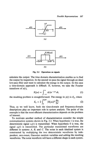
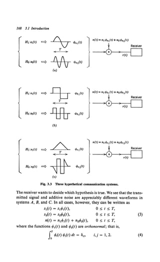
185. Series Expansions 169
The functions cp1(t) and cp2(t) are different in the three systems. It is clear
that because
r(t) = (s1 + n1) </J1(t) + n2 <P2(t),
r(t) = n1 <P1(t) + (s2 + n2) cp2(t),
0::;:;: t::;:;: T :H1 ,
0::;:;: t::;:;: T :H0, (5)
we must base our decision on the observed value of the coefficients of the
two functions. Thus the test can be viewed as
rQ [::] [~] + [::],
r Q [~:] [~J + [:J :Ho. (6)
This, however, is just a problem in classical detection that we encountered
in Chapter 2.
The important observation is that any pair of orthonormal functions
cp1(t) and cp2(t) will give the same detection performance. Therefore either
a time-domain or frequency-domain characterization will tend to obscure
the significant features of this particular problem. We refer to this third
method of characterization as an orthogonal series representation.
We develop this method of characterizing both deterministic signals and
random processes in this chapter. In the next section we discuss deter-
ministic signals.
3.2 DETERMINISTIC FUNCTIONS: ORTHOGONAL REPRESENTATIONS
Consider the function x(t) which is defined over the interval [0, T] as
shown in Fig. 3.4. We assume that the energy in the function has some
finite value Ex.
Ex = J:X 2(t) dt < 00. (7)
Now the sketch implies one way of specifying x(t). For every t we know
the value of the function x(t). Alternately, we may wish to specify x(t) by
a countable set of numbers.
The simple example in the last section suggests writing
00
x(t) = 2 X; cp;(t), (8)t
i=l
t Throughout most of our discussion we are concerned with expanding real wave-
forms using real orthonormal functions and real coefficients. The modifications to
include complex orthonormal functions and coefficients are straightforward.

186. 170 3.2 Deterministic Functions: Orthogonal Representations
x(t)
Fig. 3.4 A time-limited function.
where the cf>t(t) are some set of orthonormal functions. For example, we
could choose a set of sines and cosines
(l)Yz
c/J1(t) = T ,
(2)Yz (27T )
cp2(t) = T cos T t ,
O~t~T. (9)
(2)Yz (27T )
cp~(t) = T sin T t ,
c/J2n(t) = (jfcos e;nt)-
Several mathematical and practical questions come to mind. The mathe-
matical questions are the following:
1. Because it is only practical to use a finite number (N) of coefficients,
how should we choose the coefficients to minimize the mean-square
approximation (or representation) error?
2. As N increases, we would like the mean-square approximation error
to go to zero. When does this happen?
The practical question is this:
If we receive x(t) as a voltage waveform, how can we generate the
coefficients experimentally?
First we consider the mathematical questions. The representation error is
N
eN(t) = X(t) - L X1cp1
(t), (10)
1;1
when we use N terms. The energy in the error is
E.(N) Q JT eN2(t) dt = JT [x(t)- ~ x1cp1
(t)]
2
dt. (11)
0 0 1;1

187. Series Expansions 171
We want to minimize this energy for any N by choosing the x1 appro-
priately. By differentiating with respect to some particular x1, setting the
result equal to zero, and solving, we obtain
Xi = JOT X(t) cp1
(t) dt. (12)
Because the second derivative is a positive constant, the x1 given by (12)
provides an absolute minimum. The choice of coefficient does not change
as N is increased because of the orthonormality of the functions.
Finally, we look at the energy in the representation error as N--+ oo.
E.(N) ~ rT eN2
(t) dt = rT [x(t) - 2: XI rPI(t)] 2
dt
Jo Jo 1=1
= Ex - 2 1~ S:x(t)xl cMt) dt + JoT 1~ ~1x1
x1cMt) cfot(t) dt
(13)
Because the x12 are nonnegative, the error is a monotone-decreasing
function of N.
If, lim E.(N) = 0 (14)
N .... oo
for all x(t) with finite energy, we say that the </>1(t), i = I, ... , are a complete
orthonormal (CON) set over the interval [0, T] for the class of functions
with finite energy. The importance of completeness is clear. If we are
willing to use more coefficients, the representation error decreases. In
general, we want to be able to decrease the energy in the error to any
desired value by letting N become large enough.
We observe that for CON sets
"'
Ex = L X12• (15)
1~1
Equation 15 is just Parseval's theorem. We also observe that x12 repre-
sents the energy in a particular component of the signal.
Two possible ways of generating the coefficients are shown in Fig. 3.5.
In the first system we multiply x(t) by rMt) and integrate over [0, T].
This is referred to as a correlation operation. In the second we pass x(t)
into a set of linear filters with impulse responses hkr) = r/>1
(T- T) and
observe the outputs at time T. We see that the sampled output of the ith
filter is
LT x(T) h1
(T- T) dT.
For the particular impulse response used this is x1,
x, = LT X(T) rPt(T) dT, i = 1, 2, ... , N. (16)

188. 172 3.2 Deterministic Functions: Orthogonal Representations
x(t)
cPr,(t)
x(t)
(a)
(b)
X2
{Sample at t = T
~Xl
Fig. 3.5 Generation of expansion coefficients: (a) correlation operation;
(b) filter operation.
In Chapter 2 we saw that it was convenient to consider N observations
as a point in anN-dimensional space. We shall find that it is equally useful
to think of theN coefficients as defining a point in a space. For arbitrary
signals we may need an infinite dimensional space. Thus any finite energy
signal can be represented as a vector. In Fig. 3.6 we show two signals-
sl(t) and s2(t):
3
s1(t) = 2 su (Pt(t),
i=l
(17a)
3
s2(t) = 2 s21 if>t(t).
!=1

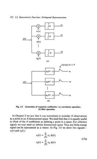
189. Geometric Representation 173
cpa~cf>a(t)
St~st(t)
Fig. 3.6 Representation of a signal as a vector.
The corresponding signal vectors are
Several observations follow immediately:
(17b)
1. The length ofthe signal vector squared equals the energy in the signal.
!s1!2= Eh
ls2l2 = E2.
2. The correlation coefficient between two signals is defined as
rT S1(t) S2(t) dt
/';.:::..Jo~----
Pl2 -- VE1E2 .
Substituting (17a) into (19), we have
P12 =
J: L~ Su ~~(t)] L~ S21 ~it)]dt
VE1E2
(18)
(19)
(20)

190. 174 3.3 Random Process Characterization
Using the orthonormality of the coordinate functions the integral
reduces to
3
LSuS21
P12 = -'-
1-,==
1 ==-
V£1£2
(21)
The numerator is just the dot product of s1 and s2• Using {18) in the
denominator, we obtain,
S1•S2
P12 = ls1l lsl (22)
The obvious advantage of the vector space interpretation is that it enables
us to use familiar geometric ideas in dealing with waveforms.
We now extend these ideas to random waveforms.
3.3 RANDOM PROCESS CHARACTERIZATION
We begin our discussion in this section by reviewing briefly how random
processes are conventionally defined and characterized.
3.3.1 Random Processes: Conventional Characterizations
The basic idea ofa random process is familiar. Each time we conduct an
experiment the outcome is a function over an interval of time instead of
just a single number. Our mathematical model is illustrated in Fig. 3.7.
Each point in the sample space n maps into a time function. We could
write the function that came from w1 as x(t, w1) to emphasize its origin, but
it is easier to denote it simply as x(t). The collection of waveforms gener-
ated from the points inn are referred to as an ensemble. Ifwe look down the
ensemble at any one time, say t1o we will have a random variable x11 £:.
x(t1o w). Similarly, at other times t1 we have random variables x1,.
Clearly, we could characterize any particular random variable x11 by its
probability density. A more difficult question is how to characterize the
entire process. There is an obvious property that this characterization
should have. If we consider a set of times t1 , t2, ••• , t.,. in the interval in
which the process is defined, there are n random variables Xt1 , Xt2 , Xt3 , ••• ,
x1n. Any complete characterization should be able to specify the joint
density Px11x12 ••• x1n(Xh X2 , ••• , X.,.). Furthermore, it should be able to
specify this density for any set of n times in the interval (for any finite n).
Unfortunately, it is not obvious that a characterization of this kind will
be adequate to answer all questions of interest about a random process.
Even if it does turn out to be adequate, there is a practical difficulty in
actually specifying these densities for an arbitrary random process.

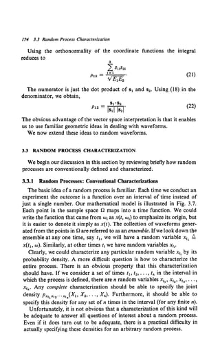
191. Random Processes: Conventional Characterizations 175
Sample space
Fig. 3.7 An ensemble of sample functions.
Outcome of
first experiment
Outcome of
second experiment
Outcome of
jlhexperiment
There are two common ways of handling this difficulty in specifying the
nth-order density.
Structured Processes. We consider only those processes in which any
nth-order density has a certain structure that can be produced by using
some low-order density and a known algorithm.
Example. Consider the probability density at the ordered set of times
l1 < l2 < Ia < ••• < ln-1 < ln.
If
the process is called a Markov process. Here knowledge of the second-order density
enables us to construct the nth order density (e.g., [2,p. 44] or Problems 3.3.9 and
3.3.10). Other structured processes will appear naturally as our discussion proceeds.
Partial Characterization. We now consider operations on the random
process that can be studied without actually completely characterizing the
process. For these operations we need only a partial characterization. A

192. 176 3.3 Random Process Characterization
large number of partial characterizations are possible. Two of the most
widely used are the following:
I. Single-time characterizations.
2. Second-moment characterizations.
In a single-time characterization we specify only Px,(X), the first-order
probability density at time t. In general, it will be a function of time. A
simple example illustrates the usefulness of this characterization.
Example. Let
r(t) = x(t) + n(t). (24)
Assume that x, and n, are statistically independent and Px,(X) and p.,(N) are
known. We operate on r(t) with a no-memory nonlinear device to obtain a minimum
mean square error estimate of x(t) which we denote by x(t).
From Chapter 2, x(t) is just the conditional mean. Because we are constrained to a
no-memory operation, we can use only r(t). Then
(25)
If x, is Gaussian, N(O, ux), and n, is Gaussian, N(O, u.), it is a simple exercise (cf.
Problem 3.3.2) to show that
,. 2
f(R,) = 2 +X 2 R.,
U;x Un
(26)
so that the no-memory device happens to be linear. Observe that because we allowed
only a no-memory device a complete characterization of the process was not necessary.
In a second-moment characterization we specify only the first and second
moments of the process. We define the mean-value function of the process
as
(27)
In general, this is a function of time. The correlation function is defined as
00
Rx(t, u) ~ E(x1xu) = JJX1XuPx,x/Xt, Xu) dXt dXu. (28)
-00
The covariance function is defined as
Kx(t, u) ~ E{[xt - mx(t)][xu - mx(u)]}
= Rx(t, u) - mx(t) mx(u). (29)
This partial characterization is well suited to linear operations on
random processes. This type of application is familiar (e.g., [1], pp. 171-
185).
The covariance function has several properties of interest to us. Looking
at the definition in (29), we see that it is symmetric:
Kx(t, u) = Kx(u, t). (30)

193. Random Processes: Conventional Characterizations 177
If we multiply a sample function x(t) by some deterministic square-
integrable functionf(t) and integrate over the interval [0, T], we obtain a
random variable:
x, ~ J:x(t) f(t) dt. (31)
The mean of this random variable is
E(x1) = x1 ~ E f x(t) f(t) dt = f mx(t) f(t) dt, (32)
and the variance is
Var (x1) ~ E[(x1 - x1) 2]
= E {f[x(t)- mx(t)] f(t) dt f [x(u)- mx(u)] f(u) du}. (33)
Bringing the expectation inside the integral, we have
T
Var (x1) = IIf(t) Kx(t, u) f(u) dt du. (34)
0
The variance must be greater than or equal to zero. Thus, we have shown
that
T
IIf(t) Kx(t, u) f(u) dt du ~ 0 (35)
0
for any f(t) with finite energy. We call this property nonnegative definite-
ness. If the inequality is strict for every f(t) with nonzero finite energy, we
say that Kx(t, u) is positive definite. We shall need the two properties in (30)
and (35) in the next section.
If the process is defined over an infinite interval and the covariance
function depends only on t - u and not tor u individually, we say that
the process is covariance-stationary and write
(36)t
Similarly, if the correlation function depends only on It - u, we say that
the process is correlation-stationary and write
(37)
t It is important to observe that although Kx(t, u) is a function of two variables and
Kx(r) of only one variable, we use the same notation for both. This economizes on
symbols and should cause no confusion.

194. 178 3.3 Random Process Characterization
For stationary processes, a characterization using the power density
spectrum Sx(w) is equivalent to the correlation function characterization
Sx(w) ~ s:"' Rx(T)e-1"'' dT
and
(38)
As already pointed out, these partial characterizations are useful only
when the operations performed on the random process are constrained to
have a certain form. A much more useful representation for the problems
of interest to us is a characterization in terms of an orthogonal series ex-
pansion. In the next section we use a series expansion to develop a second-
moment characterization. In the succeeding section we extend it to provide
a complete characterization for a particular process of interest. It is worth-
while to observe that we have yet to commit ourselves in regard to a com-
plete characterization of a random process.
3.3.2 Series Representation of Sample Functions of Random Processes
In Section 3.2 we saw how we could represent a deterministic waveform
with finite energy in terms of a series expansion. We now want to extend
these ideas to include sample functions of a random process. We start off
by choosing an arbitrary complete orthonormal set: c/>1(t), c/>2(t), .... For
the moment we shall not specify the exact form of the cfo1(t). To expand
x(t) we write
N
x(t) = lim L x1cfo1(t),
N-+a> 1=1
O::s;t::s;T, (39)
where
x1 Q LT x(t) cfo,(t) dt. (40)
We have not yet specified the type of convergence required of the sum
on the right-hand side. Various types of convergence for sequences of
random variables are discussed in the prerequisite references [1, p. 63]
or [29].
An ordinary limit is not useful because this would require establishing
conditions on the process to guarantee that every sample function could be
represented in this manner.
A more practical type of convergence is mean-square convergence:
N
x(t) = l.i.m. L x, cfo,(t),
N .... oo i=l
(41)

195. Karhunen-Loeve Expansion 179
The notation "l.i.m." denotes limit in the mean (e.g., [1, p. 63]) which is
defined as,
J~n;, E [(xt- 1~ x,<Mt)rJ = 0, 0 s t sT. (42)
For the moment we assume that we can find conditions on the process
to guarantee the convergence indicated in (42).
Before doing so we discuss an appropriate choice for the orthonormal
set. In our discussions of classical detection theory our observation space
was finite dimensional and usually came with a built-in coordinate system.
In Section 2.6 we found that problems were frequently easier to solve if we
used a new coordinate system in which the random variables were un-
correlated (if they happened to be Gaussian variables, they were also
statistically independent). In dealing with continuous waveforms we have
the advantage that there is no specified coordinate system, and therefore
we can choose one to suit our purposes. From our previous results a logical
choice is a set of <Mt) that leads to uncorrelated coefficients.
If
(43)
we would like
(44)
For simplicity we assume that m1 = 0 for all i. Several observations are
worthwhile:
I. The value x12 has a simple physical interpretation. It corresponds to
the energy along the coordinate function <Mt) in a particular sample
function.
2. Similarly, E(x12) = At corresponds to the expected value ofthe energy
along <Mt), assuming that m1 = 0. Clearly, A
1 ~ 0 for all i.
3. If Kx(t, u) is positive definite, every . is greater than zero. This
follows directly from (35). A little later it will be easy to show that if
Kx(t, u) is not positive definite, at least one A
1 must equal zero.
We now want to determine what the requirement in (44) implies about
the complete orthogonal set. Substituting (40) into (44) and bringing the
expectation inside the integral, we obtain
= J:<f,1(t) dt LT Kx(t, u) </J;(u) du, for all i and j. (45)

196. 180 3.3 Random Process Characterization
In order that (45) may hold for all choices of i and a particular j, it is
necessary and sufficient that the inner integral equal >..1 cf>it):
>..i cf>it) = J:Kx(t, u) cf>iu) du, O:$t:$T. (46)
The functions cfo1(t) are called eigenfunctions and the numbers >..1 are called
eigenvalues.
Therefore we want to demonstrate that for some useful class of random
processes there exist solutions to (46) with the desired properties. The
form of (46) is reminiscent of the equation that specified the eigenvectors
and eigenvalues in Section 2.6 {2-363),
>..cf> = Kx<f>, (47)
where Kx was a symmetric, nonnegative definite matrix. This was a set of
N simultaneous homogeneous linear equations where N was the dimen-
sionality of the observation space. Using results from linear equation
theory, we saw that there were N real, nonnegative values of>.. for which
(47) had a nontrivial solution. Now the coordinate space is infinite and we
have a homogeneous linear integral equation to solve.
The function Kx(t, u) is called the kernel of the integral equation, and
because it is a covariance function it is symmetric and nonnegative
definite. We restrict our attention to processes with a finite mean-square
value [E{x2(t)) < oo]. Their covariance functions satisfy the restriction
T 2
JJKx2(t, u) dt du ~ [ J:E[x2(t)] dt] < oo, (48)
0
where Tis a finite number.
The restrictions in the last paragraph enable us to employ standard
results from linear integral equation theoryt (e.g., Courant and Hilbert [3],
Chapter 3; Riesz and Nagy [4]; Lovitt [5]; or Tricomi [6]).
Properties ofIntegral Equations
I. There exist at least one square-integrable function cf>(t) and real
number >.. i' 0 that satisfy (46).
It is clear that there may not be more than one solution. For example,
Kx(t, u) = alf(t)f(u), 0 :$ t, u :$ T. (49)
has only one nonzero eigenvalue and one normalized eigenfunction.
2. By looking at (46) we see that if cf>1(t) is a solution then ccp1(t) is also
a solution. Therefore we can always normalize the eigenfunctions.
tHere we follow Davenport and Root [1], p. 373.

197. Properties of Integral Equations 181
3. If cfo1(t) and cfo2(t) are eigenfunctions associated with the same eigen-
value ., then c1</>1(t) + c2</>2(t) is also an eigenfunction associated with ..
4. The eigenfunctions corresponding to different eigenvalues are ortho-
gonal.
5. There is at most a countably infinite set of eigenvalues and all are
bounded.
6. For any particular . there is at most a finite number of linearly
independent eigenfunctions. [Observe that we mean algebraic linear
independence;f(t) is linearly independent of the set <f>1
(t), i = 1, 2, ... , K,
if it cannot be written as a weighted sum of the cfo1
(t).] These can always be
orthonormalized (e.g., by the Gram-Schmidt procedure; see Problem 4.2.7
in Chapter 4).
7. Because K:x(t, u) is nonnegative definite, the kernel K:x(t, u) can be
expanded in the series
00
Kx(t, u) = 2; .1 </>1(t) </>1(u),
1=1
0 ~ t, u ~ T, (50)
where the convergence is uniform for 0 ~ t, u ~ T. (This is called Mercer's
theorem.)
8. If K:x(t, u) is positive definite, the eigenfunctions form a complete
orthonormal set. From our results in Section 3.2 this implies that we can
expand any deterministic function with finite energy in terms of the
eigenfunctions.
9. If Kx(t, u) is not positive definite, the eigenfunctions cannot form a
complete orthonormal set. [This follows directly from (35) and (40).]
Frequently, we augment the eigenfunctions with enough additional ortho-
gonal functions to obtain a complete set. We occasionally refer to these
additional functions as eigenfunctions with zero eigenvalues.
10. The sum of the eigenvalues is the expected value of the energy of
the process in the interval (0, T), that is,
E [ rTx2
(t) dt] = rr K:x(t, t) dt = ~ .,.
Jo Jo 1=1
(Recall that x(t) is assumed to be zero-mean.)
These properties guarantee that we can find a set of cfo1(t) that leads to
uncorrelated coefficients. It remains to verify the assumption that we made
in (42). We denote the expected value ofthe error ifx(t) is approximated by
the first N terms as ~N(t):
~N(t)' f?= E [ (x(t) - 1~ X1 c/J1
(t))
2
]. (51)

198. 182 3.3 Random Process Characterization
Evaluating the expectation, we have
eN(t) = K,.(t, t) - 2E [x<t) I~ x, tf>,(t)] + E Lt,tx,x,tf>,(t) t/>,(t)].
(52)
eN(t) = Kx(t, t) - 2E[x(t) 1~ (fx(u) tf>,(u) du) t/>1
(t)] + ~1~tf>, (t)tf>1(t),
(53)
eN(t) = Kx(t, t) - 2 I~ u:Kx(t, u) tf>,(u) du)tf>,(t) + '~ '"tf>,(t) tf>,(t),
(54)
N
eN(t) = Kx(t, t) - L .,•Mt) cfot{t). (55)
1=1
Property 7 guarantees that the sum will converge uniformly to K,.(t, t)
as N ~ oo. Therefore
lim eN(t) = 0, 0 :s; t ::;; T, (56)
N-"'
which is the desired result. (Observe that the convergence in Property 7
implies that for any E > 0 there exists an N1 independent of t such that
eN(t) < E for all N > Nl).
The series expansion we have developed in this section is generally
referred to as the Karhunen-Loeve expansion. (Karhunen [25), Loeve [26],
p. 478, and [30].) It provides a second-moment characterization in terms
of uncorrelated random variables. This property, by itself, is not too
important. In the next section we shall find that for a particular process of
interest, the Gaussian random process, the coefficients in the expansion are
statistically independent Gaussian random variables. It is in this case that
the expansion finds its most important application.
3.3.3 Gaussian Processes
We now return to the question of a suitable complete characterization
of a random process. We shall confine our attention to Gaussian random
processes. To find a suitable definition let us recall how we defined jointly
Gaussian random variables in Section 2.6. We said that the random
variables X~o x2, ••• , xN were jointly Gaussian if
(57)
was a Gaussian random variable for any set of g1• In 2.6 N was finite and
we required the g1 to be finite. If N is countably infinite, we require the
g1 to be such that E(y2] < oo. In the random process, instead of a linear

199. Gaussian Processes 183
transformation on a set of random variables, we are interested in a linear
functional of a random function. This suggests the following definition:
Definition. Let x(t) be a random process defined over some interval [Ta, T8]
with a mean-value mx(t) and covariance function Kx(t, u). If every linear
functional of x(t) is a Gaussian random variable, then x(t) is a Gaussian
random process. In other words, if
JT8
y = g(u) x(u) du,
Ta
(58)
and g(u) is any function such that E[y2] < oo. Then, in order for x(u) to be
a Gaussian random process, y must be a Gaussian random variable for
every g(u) in the above class.
Several properties follow immediately from this definition.
Property 1. The output of a linear system is a particular linear functional
of interest. We denote the impulse response as h(t, u), the output·at time t
due to a unit impulse input at time u. If the input is x(t) which is a sample
function from a Gaussian random process, the output y(t) is also.
Proof·
J
T8
y(t) = h(t, u) x(u) du,
Ta
(59)
The interval [Tn T6 ] is simply the range over which y(t) is defined. We
assume that h(t, u) is such that E[y2(t)] < oo for all t in [Ty, T6 ]. From
the definition it is clear that y1 is a Gaussian random variable. To show
that y(t) is a Gaussian random process we must show that any linear
functional of it is a Gaussian random variable. Thus,
(60)
or
iTA JT8
z = gy(t) dt h(t, u) x(u) du,
Ty Ta
(61)
must be Gaussian for every gy(t) [such that E[z2] < oo]. Integrating with
respect to t and defining the result as
ITA
g(u) Q gy(t) h(t, u) dt,
Ty
(62)
we have
JT8
z = g(u) x(u) du,
Ta
(63)
which is Gaussian by definition.
Thus we have shown that if the input to a linear system is a Gaussian
random process the output is a Gaussian random process.

200. 184 3.3 Random Process Characterization
Property 2. If
JTP
Y1 = gl(u) x(u) du (64)
Ta
and
JTp
Y2 = g2(u) x(u) du, (65)
Ta
where x(u) is a Gaussian random process, then y1 and y2 are jointly
Gaussian. (The proof is obvious in light of (57).)
Property 3. If
(66)
and
(67)
where if>1(u) and cfolu) are orthonormalized eigenfunctions of (46) [now
the interval of interest is (Ta, T13) instead of (0, T)] then x1 and xi are stat-
istically independent Gaussian random variables (i #- j). Thus,
(68)
where
(69)
This property follows from Property 2 and (45).
Property 4. For any set of times tl> t2, t3 , ••• , tn in the interval [Ta, Tp] the
random variables x11 , x12 , ••• , x1• are jointly Gaussian random variables.
Proof If we denote the set by the vector xt>
[
Xt
1
]
!::. Xt2
Xt- . '
Xtn
(70)
whose mean is mx,
(71)

201. Gaussian Processes 185
then the joint probability density is
Px1(X) = [(21T)n'2 1AxiY.]-1 exp [-!(X- mx)TA;1{X- mJ] (72)
and the joint characteristic function is
Mxliv) = exp (jvTmx - tvTAxv), (73)
where Ax is the covariance matrix ofthe random variables x11 , x12 , ••• , x1n.
(We assume Ax is nonsingular.) The ij element is
Ax,tJ = E[(xt, - mx(tt))(Xt1 - mx(t1
))]. (74)
This property follows by using the function
n
g(u) = L g1 8(u - t1) (75)
1=1
in (58) and the result in (57). Thus we see that our definition has the de-
sirable property suggested in Section 3.3.1, for it uniquely specifies the joint
density at any set of times. Frequently Property 4 is used as the basic
definition. The disadvantage of this approach is that it is more difficult to
prove that our definition and Properties 1-3 follow from (72) than vice-
versa.
The Gaussian process we have defined has two main virtues:
1. The physical mechanisms that produce many processes are such that
a Gaussian model is appropriate.
2. The Gaussian process has many properties that make analytic
results feasible.
Discussions of physical mechanisms that lead logically to Gaussian
processes are available in [7] and [8]. Other properties of the Gaussian
process which are not necessary for our main discussion, are developed in
the problems (cf. Problems 3.3.12-3.3.18).
We shall encounter multiple processes that are jointly Gaussian. The
definition is a straightforward extension of the preceding one.
Definition. Let x1(t), x2(t), ... , xN(t) be a set of random processes defined
over the intervals (Ta1 , T13 ), (Ta2 , T132 ), ••• , (TaN' T8N), respectively. If
every sum of arbitrary functionals of x1(t), i = I, ... , N, is a Gaussian
random variable, then the processes x1(t), x2(t), ... , xN(t) are defined to
be jointly Gaussian random processes. In other words,
N rTp
y = 1~ JTa,' g1
(u) x1
(u) du
must be Gaussian for every set of g1(u) such that E[y2] < oo.

202. 186 3.4 Homogeneous Integral Equations and Eigenfunctions
Other properties of jointly Gaussian processes are discussed in the
problems.
Property 3 is the reason for our emphasis on the Karhunen-Loeve ex-
pansion. It enables us to characterize a Gaussian process in terms of an at
most countably infinite set of statistically independent Gaussian random
variables. The significance ofthis will perhaps be best appreciated when we
see how easy it makes our ensuing work. Observe that if we had chosen to
emphasize Markov processes the orthogonal expansion method of charac-
terization would not have been particularly useful. In Section 6.3 we discuss
characterizations that emphasize the Markovian structure.
The Karhunen-Loeve expansion is useful in two ways:
1. Many of our theoretical derivations use it as a tool. In the majority
ofthese cases the eigenfunctions and eigenvalues do not appear in the final
result. The integral equation that specifies them (46) need never be solved.
2. In other cases the result requires an explicit solution for one or more
eigenfunctions and eigenvalues. Here we must be able to solve the equation
exactly or find good approximate solutions.
In the next section we consider some useful situations in which solutions
can be obtained.
3.4 HOMOGENEOUS INTEGRAL EQUATIONS AND EIGENFUNCTIONS
In this section we shall study in some detail the behavior ofthe solutions
to (46). In addition to the obvious benefit of being able to solve for an
eigenfunction when it is necessary, the discussion serves several other
purposes:
1. By looking at several typical cases and finding the eigenvalues and
eigenfunctions the idea of a coordinate expansion becomes somewhat
easier to visualize.
2. In many cases we shall have to make approximations to get to the
final result. We need to develop some feeling for what can be neglected
and what is important.
3. We want to relate the behavior ofthe eigenvalues and eigenfunctions
to more familiar ideas such as the power density spectrum.
In Section 3.4.1 we illustrate a technique that is useful whenever the
random process is stationary and has a rational power density spectrum.
In Section 3.4.2 we consider bandlimited stationary processes, and in
Section 3.4.3 we look at an important nonstationary process. Next in
Section 3.4.4 we introduce the idea ofa "white" process. In Section 3.4.5,
we derive the optimum linear filter for estimating a message corrupted by

203. Rational Spectra 187
noise. Finally, in Section 3.4.6, we examine the asymptotic behavior of the
eigenfunctions and eigenvalues for large time intervals.
3.4.1 Rational Spectra
The first set of random processes of interest are stationary and have
spectra that can be written as a ratio of two polynomials in w 2•
N(w2)
Sx(w) = D(w2)' (76)
where N(w2) is a polynomial of order q in w2 and D(w2) is a polynomial of
order pin w 2 • Because we assume that x(t) has a finite mean-square value,
q < p. We refer to these spectra as rational. There is a routine but tedious
method of solution. The basic idea is straightforward. We convert the
integral equation to a differential equation whose solution can be easily
found. Then we substitute the solution back into the integral equation to
satisfy the boundary conditions. We first demonstrate the technique by
considering a simple example and then return to the general case and form-
alize the solution procedure. (Detailed discussions of similar problems are
contained in Slepian [9], Youla [10], Davenport and Root [1], Laning and
Battin [11], Darlington [12], Helstrom [13, 14], or Zadeh and Ragazzini
[22].)
Example. Let
or
2aP
Sx(w) = w• + a•, - 00 < w < oo,
- 00 < T < 00.
The mean-square value of x(t) is P. The integral equation of interest is
fTPexp(-aJt- uJ)<fo(u)du = Acp(t), -T~t~T.
(The algebra becomes less tedious with a symmetric interval.)
(77)
(78)
(79)
As indicated above, we solve the integral equation by finding the corresponding
differential equation, solving it, and substituting it back into the integral equation.
First, we rewrite (79) to eliminate the magnitude sign.
A <fo(t) = J' P exp [- a(t - u)] <fo(u)du + J.T P exp [- a(u - t)] <fo(u)du. (80)
-T t
Differentiating once, we have
A~(t) = -Para• f' e+au cp(u)du + Pae+at [T e-a• cp(u)du. (81)
-T Jt

204. 188 3.4 Homogeneous integral Equations and Eigenfunctions
Differentiating a second time gives
, ¥(t} = Pa2
fT e-«ll-ul 1>(u) du - 2Pa 1>(t);
but the first term on the right-hand side is just a2 , 1>(1). Therefore
, ~(1) = a2 , 1>(1) - 2Pa 1>(1)
or, for, >F 0,
~(I) = a 2
(, ~ 2P/a) 1>(l).
The solution to (83) has four possible forms corresponding to
(i) , = 0;
(ii) 0 < , < 2P.
"''
(iii)
2P
, =-;;
(iv) , > 2P.
"'
(82)
(83)
(84)
(85)
We can show that the integral equation cannot be satisfied for (i), (iii), and (iv).
(Cf. Problem 3.4.1.)
For (ii) we may write
0 < b2 < CX), (86)
Then
1>(1) = c1eibl + c2e-ibl. (87)
Substituting (87) into (80) and performing the integration, we obtain
0 = e-«1 1 • + 2 • - e+at 1 • + 2 • •
[
C e-<cr+Jb)T C e-Ca-Jb)T] [C e-Ca-Jb)T C e-Ca+Jb)T]
"' + }b "' - }b -"' + }b -"' - }b
(88)
We can easily verify that if c1 >F ±c2, (88) cannot be satisfied for all time. For
c1 = -c2 we require that tan bT = -bfa. For c1 = c2 we require tan bT = afb.
Combining these two equations, we have
{tan bT + ~){tan bT- ~) = 0. (89)
The values of b that satisfy (89) can be determined graphically as shown in Fig. 3.8.
The upper set of intersections correspond to the second term in (89) and the lower set
to the first term. The corresponding eigenvalues are
2Pa
"· = .....-----b
2'
a + 1
i = 1, 2, .... (90}
Observe that we have ordered the solutions to (89), b1 < b2 < ba < · · · . From (90)
we see that this orders the eigenvalues .1 > .2 > .3 • • • • The odd-numbered solutions
correspond to c1 = c2 and therefore
I
-TStST (i odd). (91)

205. Rational Spectra 189
Fig. 3.8 Graphical solution of transcendental equation.
The even-numbered solutions correspond to c1 = -c2 and therefore
-T::;; t::;; T (i even). (92)
We see that the eigenfunctions are cosines and sines whose frequencies are not
harmonically related.
Several interesting observations may be made with respect to this
example:
1. The eigenvalue corresponding to a particular eigenfunction is equal
to the height of the power density spectrum at that frequency.
2. As T increases, bn decreases monotonically and therefore An increases
monotonically.
3. As bT increases, the upper intersections occur at approximately
(i - 1) 71'/2 [i odd] and the lower intersections occur at approximately

206. 190 3.4 Homogeneous Integral Equations and Eigenfunctions
(i - 1) 7T/2 [i even]. From (91) and (92) we see that the higher index
eigenfunctions are approximately a set of periodic sines and cosines.
1 [(i - 1)7T ]
rY.(1 + si~~~Tr cos 2T t '
-T5,. t 5,_ T (i odd).
1 . [(i - 1)7T ]
rY.(l _ sin 2b1T)Y. sm 2T t '
2b1T
-T 5,_ t 5,_ T (i even).
This behavior is referred to as the asymptotic behavior.
The first observation is not true in general. In a later section (p. 204)
we shall show that the ,n are always monotonically increasing functions
ofT. We shall also show that the asymptotic behavior seen in this example
is typical of stationary processes.
Our discussion up to this point has dealt with a particular spectrum.
We now return to the general case.
It is easy to generalize the technique to arbitrary rational spectra. First
we write Sx(w) as a ratio of two polynomials,
(93)
Looking at (83), we see that the differential equation does not depend
explicitly on T. This independence is true whenever the spectrum has the
form in (93). Therefore we would obtain the same differential equation
if we started with the integral equation
, cf>(t) = J:.., Kx(t - u) cf>(u) du, -00 < t < 00. (94)
By use of Fourier transforms a formal solution to this equation follows im-
mediately:
.<l>(jw) = Sx(w) <l>(jw) = ~~::~ <l>(jw) (95)
or
(96)
There are 2p homogeneous solutions to the differential equation corres-
ponding to (96) for every value of , (corresponding to the roots of the
polynomial in the bracket). We denote them as cPh,(t, .), i = 1, ... , 2p.
To find the solution to (46) we substitute
2p
cf>(t) = L a1
c/>h,(t, ,) (97)
1=1
into the integral equation and solve for those values of , and a, that lead

207. Rational Spectra 191
to a solution. There are no conceptual difficulties, but the procedure is
tedious.t
One particular family of spectra serves as a useful model for many
physical processes and also leads to tractable solutions to the integral
equation for the problem under discussion. This is the family described by
the equation
S ( . ) = (2nP) sin (TT/2n) .
x w.n a I + (w/a)2n (98)
It is referred to as the Butterworth family and is shown in Figure 3.9.
When n = 1, we have the simple one-pole spectrum. As n increases, the
attenuation versus frequency for w > a increases more rapidly. In the
10
11"
2.0
1.0
i
S,(w:n)
---p;a
10-1
Fig. 3.9 Butterworth spectra.
t In Appendix I of Part II we shall develop a technique due to A. Baggeroer [32, 33]
that is more efficient. At the present point in our discussion we lack the necessary
background for the development.

208. 192 3.4 Homogeneous Integral Equations and Eigenfunctions
limit, as n -+ oo, we have an ideal bandlimited spectrum. In the next
section we discuss the eigenfunctions and eigenvalues for the bandlimited
spectrum.
3.4.2 Bandlimited Spectra
When the spectrum is not rational, the differential equation correspond-
ing to the integral equation will usually have time-varying coefficients.
Fortunately, in many cases of interest the resulting differential equation is
some canonical type whose solutions have been tabulated. An example in
this category is the bandlimited spectrum shown in Fig. 3.10. In this case
{
7TP
Sx(w) = --;;-'
0,
or, in cycles per second,
S,.(w) = {2~'
0,
where
27TW =a.
lwl ;s; a,
lwl >a,
Ill ;s; w,
Ill> w,
The corresponding covariance function is
K (t ) _ p sin a(t - u).
" 'u - a(t- u)
The integral equation of interest becomes
A,P(t) = P a - </>(u) du.
f+T/2 st'n (t u)
-T/2 a(t - u)
[This is just (46) with the interval shifted to simplify notation.]
(99)
(100)
(101)
(102)
(103)
Once again the procedure is to find a related differential equation and
to examine its solution. We are, however, more interested in the results
Sx(w)
P/2W
-----L=-------~------~=---~W
-21rW 21rW
Fig. 3.10 BandUmited spectrum.

209. Bandlimited Spectra 193
than the detailed techniques; therefore we merely state them ([9], [15], [16],
[17], and [18] are useful for further study).
The related differential equation over a normalized interval is
(1 - 12)/(t)- 2t/(t) + (p.- c2t 2)f(t) = 0,
where
-1 < t < 1, (104)
aT
c = "2 = 1rWT (105)
and p. is the eigenvalue. This equation has continuous solutions for certain
values of JA.(c). These solutions are called angular prolate spheroidal func-
tions and are denoted by Son(c, t), n = 0, 1, 2, .... A plot of typical
S0n(c, t) is contained in [15], [16], and [17]. These functions also satisfy
the integral equation
2[Rb1
J(c, 1)]2Son(c, t) = J+l sint<t - )u) S0n(c, u) du,
-1 c t - u
-1 :::;; t :::;; 1, (106)
or changing variables
PT[R<l>(aT 1)] 2
S (aT.:!:!...) = JT'2P sin a(t - u) S (aT 2u) d
On 2' On 2' T -T/2 a(t - u) On 2' T u,
T T
-2 ~ t ~ 2' (107)
where R'o1
J(aT/2, 1) is a radial prolate spheroidal function. Thus the eigen-
values are
n = 0, I, 2, ....
These functions are tabulated in several references (e.g. [18] or [19]).
The first several eigenvalues for various values of WT are shown in
Figs. 3.11 and 3.12. We observe a very interesting phenomenon. For
values of n > (2WT + 1) the values of ,n rapidly approach zero. We can
check the total energy in the remaining eigenvalues, for
co f+T/2
L: . = Kx(t, t) dt = PT.
i=O -T/2
(108)
In Fig. 3.11, 2WT = 2.55 and the first four eigenvalues sum to (2.54/2.55)
PT. In Fig. 3.12, 2WT = 5.10 and the first six eigenvalues sum to (5.09/
5.10)PT. This behavior is discussed in detail in [17]. Our example suggests
that the following statement is plausible. When a bandlimited process
[- W, W cps] is observed over aT-second interval, there are only (2TW+I)
significant eigenvalues.,This result will be important to us in later chapters
(specifically Chapters II-2 and II-3) when we obtain approximate solutions

210. 194 3.4 Homogeneous Integral Equations and Eigenfunctions
2WT=2.55
>-o=0.996 2~
>.1=0.912 2~
>.2=0.519 2~
>.a=O.llO 2~
- - - - ___p___ _
A4=0.009 2W
>-s = 0.0004 2"w
Fig. 3.11 Eigenvalues for a bandlimited spectrum (lWT = 1.55).
by neglecting the higher eigenfunctions. More precise statements about the
behavior are contained in [15], [16], and [17].
3.4.3 Nonstationary Processes
The process of interest is the simple Wiener process. It was developed as
a model for Brownian motion and is discussed in detail in [20] and [21].
A typical sample function is shown in Fig. 3.13.
2WT=5.10
p
>.o=l.OOO 2w
p
Al=0.999 2W
p
A2=0.997 2W
>.a=0.961 2~
>.4 =0.748 2"w
>.s = 0.321 2"w
>.6=0.061 2~
--x~:Oo6 ?w----
>.s=0.0004 iw
Fig. 3.12 Eigenvalues of a bandlimited spectrum (2WT = 5.10).

211. Nonstationary Processes 195
Fig. 3.13 Sample function of a Wiener process.
This process is defined for t ;;:::: 0 and is characterized by the following
properties:
x(O) = 0,
E[x(t)] = 0,
E[x2(t)] = a2 t,
1 ( X12
)
P:x:I(Xt) = V27Tu2t exp - 2u2t .
(109)
(110)
(111)
The increment variables are independent; that is, if t3 > t2 > t~> then
(x13 - Xt2 ) and (x12 - x1) are statistically independent. In the next
example we solve (46) for the Wiener process.
Example. Wiener Process. Using the properties of the Wiener process, we can show
that
2 • {a2u,
Kx(l, u) = a mm (u,t) = 2
at
u ~ t,
t ~ u,
In this case (46) becomes
..~(I) = J:Kx(l, u) tf>(u) du, O~t~T.
(112)
(113)

212. 196 3.4 Homogeneous Integral Equations and Eigenfunctions
Substituting (112) into (ll3)
, r/>(t) = a2 f~ u rf>(u) du + a2 t rr/>(u) du.
Proceeding as in Section 3.4.1, we differentiate (114) and obtain,
, r/>(t) = a2 f rf>(u) du.
Differentiating again, we obtain
or, for. # 0,
.. a2
r/>(t) + "I r/>(t) = 0.
There are three possible ranges for .:
(i)
(ii)
(iii)
, < 0,
. = 0,
, > 0.
(114)
(ll5)
(116)
(ll7)
(118)
We can easily verify (cf. Problem 3.4.3) that (i) and (ii) do not provide solutions that
will satisfy the integral equation. For . > 0 we proceed exactly as in the preceding
section and find
a2T2
.n = (n _ t)27T2' n=1,2, ... (119)
and
rPn(t) = (frsin [(n- ~) ft] 0::::;; t::::;; T. (120)
Once again the eigenfunctions are sinusoids.
The Wiener process is important for several reasons.
1. A large class of processes can be transformed into the Wiener process
2. A large class of processes can be generated by passing a Wiener
process through a linear or nonlinear system. (We discuss this in detail
later.)
3.4.4 White Noise Processes
Another interesting process can be derived from the Wiener process.
Using (41) and (120) we can expand x(t) in a series.
x(t) = 1;}:~·ntlXn (~)y. sin [(n - ~) ~t], (121)
where the mean-square value of the coefficient is given by {119):
(122)

213. White Noise Processes 197
We denote the K-term approximation as xK(t).
Now let us determine what happens when we differentiate xK(t):
We see that the time function inside the braces is still normalized. Thus
we may write
, K (2)Yz ( })7T
xK(t) = n~l Wn T cos n- 2 -yt, (124)
where
We observe that we have generated a process in which every eigenvalue is
equal. Clearly, if we let K--+ oo, the series would not converge. If it did, it
would correspond to a process with infinite energy over [0, T].
We can formally obtain the covariance function of this resulting process
by differentiating Kx(t, u):
()2 82 .
Kx(t, u) = ot ou Kx(t, u) = ot ou [a2 mm (t, u)]
0 ~ t, u ~ T. (125)
We see that the covariance function is an impulse. Still proceeding formally,
we can look at the solution t-o the integral equation (46) for an impulse
covariance function:
, </>(t) = a 2 s:o(t - u) </>(u) du, O<t<T. (126)
The equation is satisfied for any </>(t) with , = a 2• Thus any set of ortho-
normal functions is suitable for decomposing this process. The reason for
the nonuniqueness is that the impulse kernel is not square-integrable. The
properties stated on pp. 180--181 assumed square-integrability.
We shall find the resulting process to be a useful artifice for many
models. We summarize its properties in the following definitions.
Definition. A Gaussian white noise process is a Gaussian process whose
covariance function is a 2 8(t - u). It may be decomposed over the interval
[0, T] by using any set of orthonormal functions cPi(t). The coefficients
along each coordinate function are statistically independent Gaussian
variables with equal variance a 2 •
Some related notions follow easily.

214. 198 3.4 Homogeneous integral Equations and Eigenfunctions
Property. We can write, formally
ao
rr s(t - u) = L a 2 cMt) eMu), 0 :s; t, u :s; T. (127)
1=1
or, equivalently,
ao
8(t - u) = LcMt) eMu), 0 ~ t, u ~ T. (128)
1=1
Property. If the coefficients are uncorrelated, with equal variances, but not
Gaussian, the process is referred to as a white process.
Property. If the process is defined over the infinite interval, its spectrum is
(129)
that is, it is constant over all frequencies. The value of each eigenvalue
corresponds to the spectral height a 2•
The utility of a white noise process is parallel to that of an impulse
input in the analysis of linear systems. Just as we can observe an impulse
only after it has been through a system with some finite bandwidth, we can
observe white noise only after it has passed through a similar system.
Therefore, as long as the bandwidth ofthe noise is appreciably larger than
that of the system, it can be considered as having an infinite bandwidth.
To illustrate a typical application of eigenfunction expansions we con-
sider a simple problem.
3.4.5 The Optimum Linear Filter
In this section we consider the problem of trying to estimate a message
in the presence of interfering noise. Our treatment at this point is reason-
ably brief. We return to this problem and study it in detail in Chapter 6.
Here we have three objectives in mind:
I. The introduction of time-varying linear filters and simple minimiza-
tion techniques.
2. The development ofa specific result to be used in subsequent chapters;
specifically, the integral equation whose solution is the optimum linear
filter.
3. The illustration of how the orthogonal expansion techniques we
have just developed will enable us to obtain a formal solution to an
integral equation.
The system ofinterest is shown in Fig. 3.14. The message a(t) is a sample
function from a zero-mean random process with a finite mean-square
value and a covariance function K4 (t, u). It is corrupted by an uncorrelated

215. The Optimum Linear Filter 199
Fig. 3.14 Linear filter problem.
additive zero-mean noise n(t) with covariance function Kn(t, u). We ob-
serve the sum of these two processes,
r(t) = a(t) + n(t), 0 ::::;;; t ::::;;; T. (130)
We pass r(t) through a linear filter to obtain an estimate of a(t) denoted
by d(t).
Because a(t) is not necessarily stationary and the observation interval is
finite, we anticipate that to obtain the best estimate we may require a time-
varying filter. We characterize the filter by its impulse response h(t, u),
which is the value of the output at time t when the input is an impulse at
time u. If the system is physically realizable, then
h(t, u) = 0, t < u,
for the output cannot precede the input. If the system is time-invariant,
then h(t, u) depends only on the difference (t - u). We assume that r(t)
equals zero for t < 0 and t > T. Because the system is linear, the output
due to r(t), 0 ::::;;; t :::;; T, can be written as
a(t) = I:h(t, u) r(u) du, (131)
which is an obvious generalization of the convolution integral.
We want to choose h(t, u) to minimize the mean of the squared error
integrated over the interval [0, T]. In other words, we want to choose
h(t, u) to minimize the quantity
~~ ~ E{j., J:[a(t) - d(t)]2 dt}
= E{j., LT [a(t) - LT h(t, u) r(u) durdt} (132)
Thus we are minimizing the mean-square error integrated over the interval.
We refer to 6 as the interval estimation error.
Similarly, we can define a point estimation error:
~p(t) = E{[a(t) - s:h(t, u) r(u) dur}. 0 :::;; t :::;; T. (133)
Clearly, if we minimize the point error at each time, the total interval

216. 200 3.4 Homogeneous Integral Equations and Eigenfunctions
error will be m;nimized. One way to solve this minimization problem is to
use standard variational techniques (e.g., [31], Chapter 2). Our approach
is less formal and leads directly to a necessary and sufficient condition. We
require the filter h(t, u) to be a continuous function in both variables over
the area 0 ~ t, u ~ Tand denote the h(t, u) that minimizes ep(t) as ho(t, u).
Any other filter function h(t, u) in the allowed class can be written as
h(t, u) = h0 (t, u) + £h.(t, u), 0 ~ t, u ~ T, (134)
where " is a real parameter and h.(t, u) is in the allowable class of filters.
Taking the expectation of (133), substituting (134) into the result, and
grouping terms according to the power of "• we obtain
~p(t:£) = Ka(t. t) - 2 LT h(t, u) Ka(t, u) du
+ J:dv s:du h(t, v) h(t, u) Kr(u, v) (135)
or
~p(t:£) = Ka(t, t) - 2 LT h0 (t, u) Ka(t, u) du
+ s:dv s:du h0 (t, u) h0 (t, v) Kr(u, v)
- 2£ LT du h.(t, u) [Ka(t, u) - S:h0 (t, v) Kr(u, v) dv]
T
+ £ 2 JJh.(t, v) h.(t, u) Kr(u, v) du dv. (136)
0
If we denote the first three terms as ~p.(t) and the last two terms as
Ag(t: £), then (136) becomes
ep(t:£) = ep.(t) +Ae(t:£). (137)
Now, if h0 (t, u) is the optimum filter, then Ll~(t:£) must be greater than or
equal to zero for all allowable h.(t, u) and all " i= 0. We show that a
necessary and sufficient condition for this to be true is that
Ka(t, u) - s:h0 (t, v) Kr(u, v) dv = 0,
The equation for Ag{t: £) is
0 ~ t ~ T
O<u<T.
Ag{t: £) = -2£ s:du h.(t, u)[Ka(t, u) - LT h0 (t, v) Kr(u, v) dv]
T
+ £ 2 ffh.(t, v) h.(t, u) Kr(u, v) du dv.
0
(138)
(139)

217. The Optimum Linear Filter 201
Three observations are needed:
I. The second term is nonnegative for any choice of h,(t, v) and e
because K,(t, u) is nonnegative definite.
2. Unless
f h,(t, u) [Ka(t, u) - f h0 (t, v) K,(u, v) dv] du = 0, (140)
there exists for every continuous h,(t, u) a range of values of e that will
cause ~W: oo) to be negative. Specifically, ~g{t: e) < 0 for all
2lTh,(t, u) [Ka(t, u) - rh0 (t, v) K,(u, v) dv] du
0 < E < O T O (141)
IIh,(t, v) h,(t, u) K,(u, v) du dv
0
if the numerator on the right side of (141) is positive. ~g{t:e) is negative
for all negative e greater than the right side of (141) if the numerator is
negative.
3. In order that (140) may hold, it is necessary and sufficient that the
term in the bracket be identically zero for all 0 < u < T. Thus
rT o< t < r
Ka(t, u) - Jo h0 (t, v) K,(u, v) dv = 0, 0 ~ u-::: T. (142)
The inequality on u is strict if there is a white noise component in r(t)
because the second term is discontinuous at u = 0 and u = T. If (142) is
not true, we can make the left side of(l40) positive by choosing h,(t, u) > 0
for those values of u in which the left side of (142) is greater than zero and
h,(t, u) < 0 elsewhere. These three observations complete the proofof(138).
The result in (138) is fundamental to many ofour later problems. For the
case of current interest we assume that the additive noise is white. Then
K,(t, u) = ~o o(t - u) + Ka(t, u).
Substituting (143) into (138), we obtain
N, r
2°h0 (t, u) + Jo h0 (t, v) Ka(u, v) dv = Ka(t, u),
0 ~ t ~ T
O<u<T.
(143)
(144)
Observe that h0 (t, 0) and h0 (t, T) are uniquely specified by the continuity
requirement
h0(t, 0) = lim h0(t, u)
u-+O+
h0 (t, T) = lim h0 (t, u).
u-+T-
(145a)
(145b)

218. 202 3.4 Homogeneous Integral Equations and Eigenfunctions
Because a(t) has a finite mean-square value, (145a) and (145b) imply that
(144) is also valid for u = 0 and u = T.
The resulting error for the optimum processor follows easily. It is simply
the first term in (137).
~p.(t) = K4
(t, t) - 2 JoT h0
(t, u) K4
(t, u) du
T
+ JJh0(t, u) h0(t, v) Kr(u, v) du dv (146)
0
or
~p.(t) = K4 (t, t) - LT h.(t, u) Ka.(t, u) du
- J: h.(t, u)[Ka.(t, u) - JoT h.(t, v) Kr(u, v) dv] du. (147)
But (138) implies that the term in brackets is zero. Therefore
~p.(t) = Ka.(t, t) - LT h0(t, u) Ka.(t, u) du. (148)
For the white noise case, substitution of (144) into (148) gives
(149)
As a final result in our present discussion of optimum linear filters, we
demonstrate how to obtain a solution to {144) in terms of the eigenvalues
and eigenfunctions of K4 (t, u). We begin by expanding the message
covariance function in a series,
..
Ka.(t, u) = L: ~·Mt) t/>1(u), (150)
1=1
where .1 and cfot(t) are solutions to (46) when the kernel is K4 (t, u). Using
(127), we can expand the white noise component in (143)
Kw(t, u) = ~o a(t - u) = ~ ~o t/>1(t) t/>,(u). (151)
1=1
To expand the white noise we need a CON set. If K4 (t, u) is not positive
definite we augment its eigenfunctions to obtain a CON set. (See Property 9
on p. 181).
Then
"" ( No)
Kt(t, u) = 1~ ~ + T t/>1(t) t/>1(u). (152)

219. The Optimum Linear Filter 203
Because the tMt) are a CON set, we try a solution of the form
ao
ho(t, u) = Lh1 tMt) 4>t(u). (153)
jml
Substituting (150), (152), and (153) into (144), we find
ao ~~
h0 (t, u) = L: ~ N, 12 4>t(t) 4>t(u).
1=1 + 0
(154)
Thus the optimum linear filter can be expressed in terms of the eigen-
functions and eigenvalues of the message covariance function. A K-term
approximation is shown in Fig. 3.15.
The nonrealizability could be eliminated by a T-second delay in the
second multiplication. Observe that (154) represents a practical solution
only when the number of significant eigenvalues is small. In most cases
the solution in terms of eigenfunctions will be useful only for theoretical
purposes. When we study filtering and estimation in detail in later chapters,
we shall find more practical solutions.
The error can also be expressed easily in terms ofeigenvalues and eigen-
functions. Substitution of (154) into (149) gives
0 ~ t ~ T (155)
and
(156)
Fig. 3.15 Optimum filter.

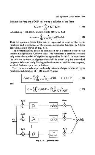
220. 204 3.4 Homogeneous Integral Equations and Eigenfunctions
In addition to the development of a useful result, this problem has
provided an excellent example of the use of eigenfunctions and eigenvalues
in finding a series solution to an integral equation. It is worthwhile to re-
emphasize that all the results in this section were based on the original
constraint of a linear processor and that a Gaussian assumption was not
needed. We now return to the general discussion and develop several
properties of interest.
3.4.6 Properties of Eigenfunctions and Eigenvalues
In this section we derive two interesting properties that will be useful in
the sequel.
Monotonic Property.t Consider the integral equation
A
1(T) 4>1(t:T) = LT Kx(t, u) 4>1(u:T) du, 0::;; t::;; T, (157)
where Kx(t, u) is a square-integrable covariance function. [This is just (46)
rewritten to emphasize the dependence of the solution on T.] Every eigen-
value ,1(T) is a monotone-increasing function ofthe length ofthe interval T.
Proof Multiplying both sides by 4>1(t:T) and integrating with respect to t
over the interval [0, T], we have,
T
1
(T) = If4>t(t: T) Kx(t, u) 4>1(u: T) dt du. (158)
0
Differentiating with respect to T we have,
o>.I(T) =2 fTo</>t(t:T)d rK( ).1.( ·T)d
oT Jo oT t Jo xt,u ~~u. u
+ 2tPt(T:T) s:Kx(T, u) 4>1(u:T) du. (159)
Using (157), we obtain
(),~'?) = 2-(T) s:o4>~~~T) 4>1(t:T) dt + 2A1(T) 4>12(T:T). (160
To reduce this equation, recall that
LT 4>t2(t: T) dt = 1.
t This result is due to R. Huang [23].
(161)

221. Properties of Eigenfunctions and Eigenvalues 205
Differentiation of (161) gives
2 J:o!/J~~~T) cf>t(t: T) dt + !/J12(T: T) = 0.
By substituting (162) into (160), we obtain
a>..~<:) = >..t(T) !/Jt2(T:T) ~ 0,
which is the desired result.
(162)
(163)
The second property of interest is the behavior of the eigenfunctions and
eigenvalues of stationary processes for large T.
Asymptotic Behavior Properties. In many cases we are dealing with
stationary processes and are interested in characterizing them over an
infinite interval. To study the behavior of the eigenfunctions and eigen-
values we return to (46); we assume that the process is stationary and that
the observation interval is infinite. Then (46) becomes
>.. !/J(t) = J~.., Kx(t - u) !/J(u) du, - oo < t < oo. (164)
In order to complete the solution by inspection, we recall the simple
linear filtering problem shown in Figure 3.16. The input is y(t), the impulse
response is h(r), and the output is z(t). They are related by the convolution
integral:
z(t) = J~.., h(t - u) y(u) du, -00 < t < 00. {165)
In a comparison of (164) and (165) we see that the solution to {164) is
simply a function that, when put into a linear system with impulse response
Kx(r), will come out of the system unaltered except for a gain change. It is
well known from elementary linear circuit theory that complex exponen-
tials meet this requirement. Thus
!/J(t) = ei"'1, -00 < w < oo, {166)t
y (t) ,. 81--z(_t)_),_
Fig. 3.16 Linear filter.
t The function e<•+i.,>< also satisfies (165) for values of u where the exponential
transform of h(T) exists. The family of exponentials with u = 0 is adequate for our
purposes. This is our first use of a complex eigenfunction. As indicated at the begin-
ning of Section 3.2, the modifications should be clear. (See Problem 3.4.11)

222. 206 3.4 Homogeneous Integral Equations and Eigenfunctions
is an eigenfunction for any w on the real line. Substituting into (164), we
have
(167)
or
.. = s:"' Kx(t - u)e-1"'<t-u> du = Sx(w). (168)
Thus the eigenvalue for a particular w is the value of the power density
spectrum of the process at that w.
Now the only difficulty with this discussion is that we no longer have a
countable set of eigenvalues and eigenfunctions to deal with and the idea
of a series expansion of the sample function loses its meaning. There are
two possible ways to get out of this difficulty.
I. Instead oftrying to use a series representation ofthe sample functions,
we could try to find some integral representation. The transition would be
analogous to the Fourier series-Fourier integral transition for deterministic
functions.
2. Instead ofstarting with the infinite interval, we could consider a finite
interval and investigate the behavior as the length increases. This might
lead to some simple approximate expressions for large T.
In Sections 3.5 and 3.6 we develop the first approach. It is an approach
for dealing with the infinite interval that can be made rigorous. The second,
which we now demonstrate, is definitely heuristic but leads to the correct
results and is easy to apply.
We start with (46) and assume that the limits are -T/2 and T/2:
f+T/2 T T
, tfo(t) = -T/
2
Kx(t - u) tfo(u) du, - 2 :::; t :::; 2.
We define
I
fo = r'
and try a solution of the form,
cPn(u) = e+i2nfonu, T T
--<u<-,
2- -2
(I69)
(170)
(171)
where n = 0, ±I, ± 2, .... (We index over both positive and negative
integers for convenience).
Define
fn = nfo·
Substituting (17I) into (169), we have
JT/2
..n tPn(t) = Kx(t - u)e+12"1nu du.
-T/2
(I72)
(I73)

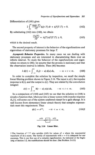
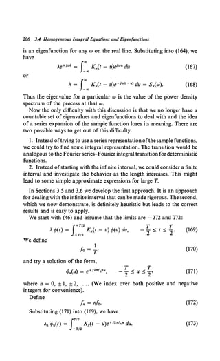
223. Properties of Eigenfunctions and Eigenvalues 207
Now,
Kx(t - u) = s:oo Sx(f)e+J2nf<t-u> df (174)
Substituting (174) into (173) and integrating with respect to u, we obtain
An cfon(t) = s:oo Sx(f)e+12"11[sin1TC~(~ //)] df (175)
The function in the bracket, shown in Fig. 3.17, is centered at f = fn
where its height is T. Its width is inversely proportional to T and its area
equals one for all values ofT. We see that for large T the function in the
bracket is approximately an impulse at fn· Thus
An cf>n(t) ~ J:"" Sx(f)e+12" 11 o(f- fn) df = Sx(fn)e+12"'•t. (176)
Therefore
and
for large T.
T T
-- < t < -·
2- - 2
(177)
(178)
From (175) we see that the magnitude of Tneeded for the approximation
to be valid depends on how quickly Sx(f) varies near fn·
In (156) we encountered the infinite sum of a function of the eigenvalues
gl =No I At .
2Tt=l,i + N0 /2
(179)
More generally we encounter sums of the form
00
g" ~ 2 g(,;). (180)
i=l
An approximate expression for g" useful for large T follows directly
from the above results. In Fig. 3.18 we sketch a typical spectrum and the
approximate eigenvalues based on (177). We see that
+oo +oo
g" ~ :2 g(Sx(nfo)) = T :2 g(Sx(nfo))fo, (181)
where the second equality follows from the definition in (170). Now, for
large T we can approximate the sum by an integral,
(182)
which is the desired result.

224. 208 3.4 Homogeneous Integral Equations and Eigenfunctions
T
sin rT(fn- ()
.,.-(fn- f)
Fig, 3.17 Weighting function in (175).
The next properties concern the size of the largest eigenvalue.
Maximum and Minimum Properties. Let x(t) be a stationary random pro-
cess represented over an interval of length T. The largest eigenvalue
Ama.x(T) satisfies the inequality
Amax(T) ~ max Sx(f)
f
for any interval T. This result is obtained by combining (177) with the
monotonicity property.
Another bound on the maximum eigenvalue follows directly from
Property 10 on p. 181.
J
n2 J®
Ama.x(T) ~ Kx(t, t) dt = T Sx(j) df.
-T/2 - ®
Fig. 3.18 Approximate eigenvalues; large T.

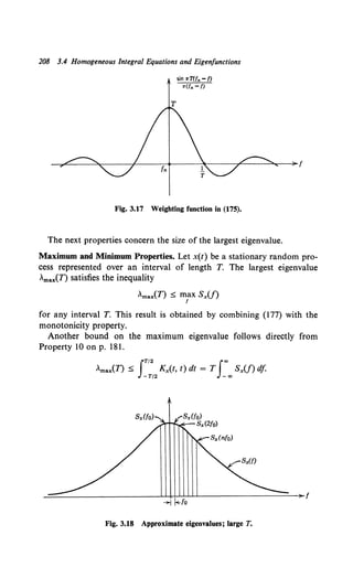
225. Cosine-Sine Expansion 209
A lower bound is derived in Problem 3.4.4,
T/2
Amax(T) ~ f f!(t) Kx(t, u)f(u) dt du,
-T/2
wheref(t) is any function with unit energy in the interval (- T/2, T/2).
The asymptotic properties developed on pp. 205-207 are adequate for
most of our work. In many cases, however, we shall want a less heuristic
method of dealing with stationary processes and an infinite interval.
In Section 3.6 we develop a method of characterization suitable to
stationary processes over an infinite interval. A convenient way to approach
this problem is as a limiting case ofa periodic process. Therefore in Section
3.5 we digress briefly and develop representations for periodic processes.
3.5 PERIODIC PROCESSESt
Up to this point we have emphasized the representation ofprocesses over
a finite time interval. It is often convenient, however, to consider the infinite
time interval. We begin our discussion with the definition of a periodic
process.
Definition. A periodic process is a stationaryrandom process whose correla-
tion function Rx(T) is periodic with period T:
for all T.
It is easy to show that this definition implies that almost every sample
function is periodic [i.e., x(t) = x(t + T)]. The expectation of the
difference is
E[(x(t) - x(t + T))2] = 2Rx(O) - 2Rx(T) = 0.
Therefore the probability that x(t) = x(t + T) is one.
We want to represent x(t) in terms ofa conventional Fourier series with
random coefficients. We first consider a cosine-sine series and assume that
the process is zero-mean for notational simplicity.
Cosine-Sine Expansion. The series expansion for the process is
x(t) = lNi..:.~·~~ [Xcl cos e;it) + x., sin (2
; it)]' - 00 < t < oo, {183)
t Sections 3.5 and 3.6 are not essential to most of the discussions in the sequel and
may be omitted in the first reading.

226. 210 3.5 Periodic Processes
where
2 JT/2 (2'1T )
Xct = T -T/2 x(t) cos Tit dt (184)
and
x,, = j.f~~2 x(t) sin c;it) dt. (185)
The covariance function can be expanded as
(186)
where
2 JT/2 (2'1T )
p, = T -T/2 Kx(T) cos TiT dT. (187)
It follows easily that
E(xc,Xc1) = E(x.,x.1) = 0, i =F j,
(188)
all i,j.
Thus the coefficients in the series expansion are uncorrelated random
variables. (This means that the eigenfunctions of any periodic process for
the interval (- T/2, T/2) are harmonically related cosines and sines.)
Similarly,
(189)
Observe that we have not normalized the coordinate functions. The motiva-
tion for this is based on the fact that the power, not the energy, at a given
frequency is the quantity ofinterest. By omitting the v'fin the coordinate
functions the value (xc12 + xs~2) represents the power and not the energy.
The expected value of the power at frequency w1 £ 21ri/T £ iw0 is p1•
Complex Exponential Expansion. Alternately, we could expand the
process by using complex exponentials:
and
K ( ) ~ p, ( . 2'1T . )
x -r = ,="="' 2 exp 1 T zt ,
,,.0
x(t) = l.i.m. 'f x, exp (j2
T'" u),
N-HIJ t= -N
, .. 0
-00 < t < oo.
For positive i,
i '2:::. 1.
(190)
(191)
(192)

227. Spectral Decomposition 211
Xci = 2 Re (xi)
' '
I I
I
'
I
' I I
I I I I
T I I I
' t I
I I I I I
' I
w w
211'" 411'" I 1011'" 211'" 411'" 611'" I 1011'"
r r ~ 1' T r T ~ 1'
(a) (b)
Fig. 3.19 Coefficients for a typical sample function.
The values for negative indices are conjugates of the values for positive
indices:
and
x1 = ~f:,2 x(t) exp ( -j 2
; it) dt.
We see that the coefficients are uncorrelated.
(193)
(194)
(195)
Just as in the finite interval case, every sample function is determined
in the mean-square sense by its coefficients. We can conveniently catalog
these coefficients as a function of w. In Fig. 3.19 we show them for a
typical sample function. In Fig. 3.20 we show the statistical average of the
square of the coefficients (the variance).
Pi
' T
'
I
•
I I I I •
'
I I I
•
I I I I I
211'" 1011'" 1411'"
w
T T T
Fig. 3.20 Variance of coefficients: periodic process.

228. 212 3.6 Infinite Interval: Spectral Decomposition
3.6 INFINITE TIME INTERVAL: SPECTRAL DECOMPOSITION
3.6.1 Spectral Decomposition
We now consider the effect of letting T, the period of the process,
approach infinity.
Cosine-Sine Representation. Looking at Fig. 3.19, we see that the lines
come closer together as T increases. In anticipation of this behavior, a
more convenient sketch might be the cumulative amplitude plot shown in
Fig. 3.21 for a typical sample function. The function z.(w,.) is the sum of
the cosine coefficients from 1 through w,.( ~ nw0).
Similarly,
"
z.(w,.) = L Xcl•
1=1
n
z.cw,.) = L: x.~.
1•1
We see that because of the zero-mean assumption,
z.co) = z.(o) = o,
and
n n 2 IT/2
z.(w,.) = L Xcl = L -T x(t) cos (iwot) dt.
1=1 1=1 -T/2
Fig. 3.21 Cumulative voltage function: periodic process.
(196)
(197)
(198)
(199)

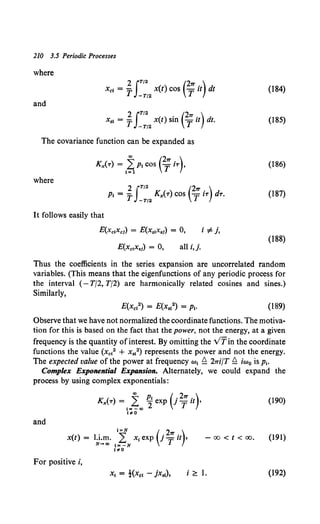
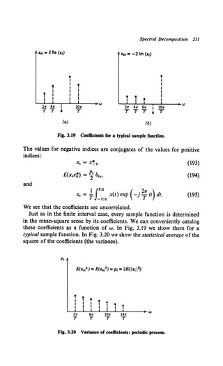
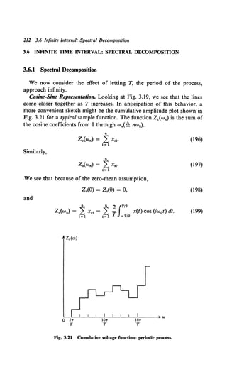
229. Spectral Decomposition 213
Looking at (183), we see that we can write
N
x(t) = l.i.m. 2: [Z.(wn) - Z0 (wn-1)] COS Wnt
N-+oo n=l
N
+ l.i.m. 2 [Z.(wn)- z.(wn-1)] sin Wnt. (200)
N-+oo n=l
From the way it is defined we see that
E{[Z.(wn) - Z.(wn-1)]2} = E{[Z.(wn) - Z.(wn-1)]2} = Pn· (201)
We can indicate the cumulative mean power by the function G.(wn),
where
n
G.(wn) = 2Pt = Gs(wn),
1=1
(202)
A typical function is shown in Fig. 3.22.
The covariance function can be expressed in terms of G.(wn) by use of
(186) and (202).
co
K,c{T) = 2 [Gc(wn) - Gc(Wn-1)] COS WnT• (203)
n=1
Complex Exponential Representation. Alternately, in complex notation,
n n 1 JT/2
Z(wn) - Z(wm) = 2 Xt = 2 - x(t)e-f<troo>t dt
t=m+1 t=m+1 T -T/2
and
N
x(t) = l.i.m. L [Z(wn)- Z(wn-1)]ei"'nt,
N-+00 n= -N
{204)
~~-L----------~------------------~w
211" 411" 21rn
'T'T 1'
Fig. 3.22 Cumulative power spectrum: periodic process.

230. 214 3.6 Infinite Interval: Spectral Decomposition
The mean-square value of the nth coefficient is,
n = -oo, ... , -1, 1, ... ,oo, (205)
The cumulative mean power is,
" p
G(w,.) = 2: J'
I=- oo
w,. > -oo, (206)
and
K,.(-r) = .i [G(w,.)- G(w,._1)]e1"'n'. (207)
n= -®
Cosine-Sine Representation. We now return to the cosine-sine repre-
sentation and look at the effect ofletting T-+ oo. First reverse the order of
summation and integration in (199). This gives
JT/2 II 1
Zc(w,.) = 2x(t) 2: cos (iw0 t) -T dt.
-T/2 1=1
(208)
Now let
liw 1
-2 =llf= -·
7T T
and
w = nw0 = w,..
Holding nw0 constant and letting T-+ oo, we obtain
Joo f"' dw
Zc(w) = _00
2x(t) dt Jo COS wt 27T (209)
or
1 foo sin wt
Zc(w) = -
2 2 - - x(t) dt.
7T -co I
(210)
Similarly,
Z,(w) = 2~ I-oooo 2 I - ~OS wt x(t) dt. (211)
The sum representing x(t) also becomes an integral,
x(t) ~ Leo dZc(w) cos wt + Loo dZ,(w) sin wt. (212)
We have written these integrals as Stieltjes integrals. They are defined as
the limit of the sum in (200) as T-+ oo. It is worthwhile to note that we
shall never be interested in evaluating a Stieltjes integral. Typical plots
of Zc(w) and Z.(w) are shown in Fig. 3.23. They are zero-mean processes
with the following useful properties:

231. Spectral Decomposition 215
Zc(W) z.(w)
Fig. 3.23 Typical integrated voltage spectrum.
1. The increments in disjoint intervals are uncorrelated; that is,
E{[Z.(w1) - z.(w1 - dw1)][Z.(w2) - Z.(w2 - dw2)]} = 0 (213)
and
E{[Z,(w1) - Z.(w1 - dw1)][Z.(w2) - z.(w2 - dw2)]} = 0 (214)
if (w1 - dwl> wd and (w2 - dw2, w2 ] are disjoint. This result is directly
analogous to the coefficients in a series expansion being uncorrelated.
2. The quadrature components are uncorrelated even in the same
interval; that is,
E{[Z.(w1) - z.(w1 - dw1)J[Z,(w2) - Z,(w2 - dw2)]} = 0 (215)
for all w1 and w2•
3. The mean-square value of the increment variable has a simple
physical interpretation,
E{[Z.(w1) - z.(w1 - dw)]2} = G.(w1) - G.(w1 - dw). (216)
The quantity on the right represents the mean power contained in the
frequency interval (w1 -!l.w, wd.
4. In many cases of interest the function G.(w) is differentiable.
(217)
(The "2" inside the integral is present because Sx(w) is a double-sided
spectrum.)
dG.(w) b. 2Sx(w).
dw - 21T
(218)
5. Ifx(t) contains a periodic component offrequency "'•• G.(w) will have
a step discontinuity at "'• and Sx{w) will contain an impulse at "'•·
The functions Z.(w) and z.(w) are referred to as the integrated Fourier
transforms of x(t). The function G0(w) is the integrated spectrum of x(t).
A logical question is: why did we use z.(w) instead of the usual Fourier
transform of x(t)?

232. 216 3.6 Infinite Interval: Spectral Decomposition
The difficulty with the ordinary Fourier transform can be shown. We
define
JT/2
Xc,T(w) = x(t) COS wt dt
-T/2
and examine the behavior as T-+ oo. Assuming E[x(t)] = 0,
E[Xc,T(w)] = 0,
and
(219)
(220)
J
T/2 JT/2
E[JXc,T(w)i2] = dt du Rx(t- u) cos wt cos wu. (221)
-T/2 -T/2
Itis easy to demonstrate that the right side of(221) will become arbitrarily
large as T-+ oo. Thus, for every w, the usual Fourier transform is a
random variable with an unbounded variance.
Complex Exponential Representation. A similar result to that in (210)
can be obtained for the complex representation.
1 Joo (e-1w.t _e-iw,.t)
Z(wn) - Z(wm) = -
2 _ . x(t) dt
1T - 00 }t
(222)
and
x(t) = J:"' dZ(w)e1
wt. (223)
The expression in (222) has a simple physical interpretation. Consider the
complex bandpass filter and its transfer function shown in Fig. 3.24. The
impulse response is complex:
The output at t = 0 is
J"' 1 (e-1w.• _ e-iw,.•)
y(O) = -
2 _. x(r) dr = Z(wm)- Z(wn)·
- oo 1T jT
x(t)
..
4 H8 (jw)= 0
hg (T)
y(t)
)
D
Fig. 3.24 A complex filter.
:>w
(224)
(225)

233. Spectral Decomposition 217
Thus the increment variables in the Z(w) process correspond to the output
of a complex linear filter when its input is x(t).
The properties of interest are directly analogous to (213)-(218) and are
listed below :
E[JZ(w) - Z(w - ~w)J 2 ] = G(w) - G(w - ~w). {226)
If G{w) is differentiable, then
dG(w) I.J. Sx(w). (227)
dw - 2'7T
A typical case is shown in Fig. 3.25.
E{JZ(w) - Z(w - ~w)J2} = 2
1 (w Sx(w) dw. (228)
'IT Jw-11w
If w 3 > w 2 > wl> then
E{[Z(w3) - Z(w2)][Z*(w2) - Z*(w1)]} = 0. (229)
In other words, the increment variables are uncorrelated. These proper-
ties can be obtained as limiting relations from the exponential series or
directly from (225) using the second-moment relations for a linear
system.
Several observations will be useful in the sequel:
l. The quantity dZ(w) plays exactly the same role as the Fourier trans-
form of a finite energy signal.
For example, consider the linear system shown in Fig. 3.26. Now,
y(t) = J_'»oo h(T) X(t - T) dT (230)
or
J_"'"' dZ11(w)eiwt = f_"'"' dT h(T) J_"'"' dZx(w)eiw<t-•> (231)
G(w) S,.(w)
Fig. 3.25 An integrated power spectrum and a power spectrum.

234. 218 3.6 Infinite Interval: Spectral Decomposition
x(t) y(t)
Fig. 3.26 Linear filter.
Thus
dZy{w) = H(jw) dZx(w) (233)
and
(234)
2. Ifthe process is Gaussian, the random variables [Z(w1)- Z(w1 - dw)]
and [Z(w2) - Z(w2 - dw)] are statistically independent whenever the
intervals are disjoint.
We see that the spectral decompositiont ofthe process accomplishes the
same result for stationary processes over the infinite interval that the
Karhunen-Loeve decomposition did for the finite interval. It provides us
with a function Z(w) associated with each sample function. Moreover, we
can divide the w axis into arbitrary nonoverlapping frequency intervals;
the resulting increment random variables are uncorrelated (or statistically
independent in the Gaussian case).
To illustrate the application of these notions we consider a simple
estimation problem.
3.6.2 An Application of Spectral Decomposition: MAP Estimation of a
Gaussian Process
Consider the simple system shown in Fig. 3.27:
r(t) = a(t) + n(t), -oo < t < oo. (235)
We assume that a(t) is a message that we want to estimate. In terms of the
integrated transform,
-00 < w < 00. (236)
r(t)
a(t) )'0 r(t) )
Fig. 3.27 System for estimation example.
t Further discussion of spectral decomposition is available in Gnedenko [27] or
Bartlett ([28], Section 6-2).

235. Application of Spectral Decomposition 219
Assume that a(t) and n(t) are sample functions from uncorrelated zero-
mean Gaussian random processes with spectral densities Sa(w) and S,.(w),
respectively. Because Za(w) and Z,.(w) are linear functionals of a Gaussian
process, they also are Gaussian processes.
Ifwe divide the frequency axis into a set of disjoint intervals, the incre-
ment variables will be independent. (See Fig. 3.28.) Now consider a
particular interval (w - dw, w] whose length is dw. Denote the increment
variables for this interval as dZ,(w) and dZ,.(w). Because of the statistical
independence, we can estimate each increment variable, dZa(w), separately,
and because MAP and MMSE estimation commute over linear trans-
formations it is equivalent to estimating a(t).
The a posteriori probability of dZa(w), given that dZ,(w) was received,
is just
PdZ.,(OJ)IdZr(OJ)[dZa(w)ldZr(w)]
= k ex (-! ldZ,(w) - dZa(w)i 2 _ ! ldZa(w)l2 )· ( 237)
p 2 S,.(w) dw/2TT 2 Sa(w) dw/2TT
[This is simply (2-141) with N = 2 because dZ,(w) is complex.]
Because the a posteriori density is Gaussian, the MAP and MMSE
estimates coincide. The solution is easily found by completing the square
and recognizing the conditional mean. This gives
/"'-.. Sa(w)
dZ4(w) = dZa(w) = Sa(w) + S,.(w) dZ,(w). (238)
Therefore the minimum-mean square error estimate is obtained by
passing r(t) through a linear filter,
H U ) Sa(w) (239)
0 w = Sa(w) + S,.(w)·
We see that the Gaussian assumption and MMSE criterion lead to a
linear filter. In the model in Section 3.4.5 we required linearity but did not
assume Gaussianness. Clearly, the two filters should be identical. To
verify this, we take the limit of the finite time interval result. For the
special case of white noise we can modify the result in (154) to take in
account the complex eigenfunctions and the doubly infinite sum. The
result is,
ho(t, u) = t=%"' >., +>.~o/2 tfo,(t) tfot(u). (240)
Using (177) and (178), we have
1• h ( ) 2 Jao Sa(w) { ) dw
1m o f, U = s ( ) AT
12 COS W ( - U -2>
T-+oo o aW +lYo 7T
(241)
which corresponds to (239).

236. 220 3.7 Vector Random Processes
- +-dw
Fig. 3.28 Integrated transforms of a(t) and r(t).
In most of our developments we consider a finite time interval and use
the orthogonal series expansion of Section 3.3. Then, to include the infinite
interval-stationary process case we use the asymptotic results of Section
3.4.6. This leads us heuristically to the correct answer for infinite time. A
rigorous approach for the infinite interval would require the use of the
integrated transform technique we have just developed.
Before summarizing the results in this chapter, we discuss briefly how
the results of Section 3.3 can be extended to vector random processes.
3.7 VECTOR RANDOM PROCESSES
In many cases of practical importance we are concerned with more than
one random process at the same time; for example, in the phased arrays
used in radar systems the input at each element must be considered.
Analogous problems are present in sonar arrays and seismic arrays in
which the received signal has a number of components. In telemetry
systems a number of messages are sent simultaneously.
In all of these cases it is convenient to work with a single vector random
process x(t) whose components are the processes of interest. If there are
N processes, x1(t), x2(t)· · ·xN(t), we define x(t) as a column matrix,
[
xl(t)l
x2(t)
x(t) ~ ; .
xN(t)
(242)

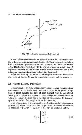
237. Vector Eigenfunctions, Scalar Eigenvalues 221
The dimension N may be finite or countably infinite. Just as in the single
process case, the second moment properties are described by the process
means and covariance functions. In addition, the cross-covariance
functions between the various processes must be known. The mean value
function is a vector
mx(t) ~£[:~:~] = [::::~].
xN(t) mN(t)
(243)
and the covariances may be described by an N x N matrix, Kx(t, u), whose
elements are
Ku(t, u) ~ E{[x1
(t) - m1(t)][x1(u) - m;(u)]}. (244)
We want to derive a series expansion for the vector random process x(t).
There are several possible representations, but two seem particularly
efficient. In the first method we use a set of vector functions as coordinate
functions and have scalar coefficients. In the second method we use a set
of scalar functions as coordinate functions and have vector coefficients.
For the first method and finite N, the modification of the properties on
pp. 180-181 is straightforward. For infinite N we must be more careful.
A detailed derivation that is valid for infinite N is given in [24]. In the
text we go through some of the details for finite N. In Chapter II-5 we
use the infinite N result without proof. For the second method, additional
restrictions are needed. Once again we consider zero-mean processes.
Method 1. Vector Eigenfunctions, Scalar Eigenvalues. Let
N
x(t) = l.i.m. Lx,«t»1(t),
N-+oo 1=1
(245)
where
iT iT NiT
x1 = «t»t(t) x(t) dt = xT(t) ct»1(t) dt = L xk(t) cfol(t) dt, (246)
0 0 k=l 0
and
(247)
is chosen to satisfy
0'5.t'5.T. (248)

238. 222 3.7 Vector Random Processes
Observe that the eigenfunctions are vectors but that the eigenvalues are
still scalars.
Equation 248 can also be written as,
~J: Kkit, u) tfo/(u) du = "A1tfo8t), k:::; 1, ... , N, 0 ~ t ~ T. (249)
The scalar properties carry over directly. In particular,
E(x1x1) = .181"
and the coordinate functions are orthonormal; that is,
or
N rT
k~ Jo tfoNt) tfo/(t) dt = SIJ•
The matrix
Kx(t, u) = E[x(t) xT(u)] - mx(t) mxT(u)
00 00
= L: L: Cov [x1
x1] cf>t(t) cf>l(u)
1=1 1=1
""
= L: "A,cf>1
(t)cf>{(u)
1=1
or
00
(250)
(251)
(252)
(253)
Kx,kit, u) = L: AttfoNt) tfo/(u), k,j = l, ... , N. (254)
1=1
This is the multidimensional analog of (50).
One property that makes the expansion useful is that the coefficient is a
scalar variable and not a vector. This point is perhaps intuitively trouble-
some. A trivial example shows how it comes about.
Example. Let
x1(t) = a s1(t),
x2(t) = b s2(t),
O::;;t::;;T,
O~t~T.
(255)
where a and bare independent, zero-mean random variables and s1(t) and
s2(t) are orthonormal functions
and
J:St(t) slt) dt = Slf,
Var (a) = aa2,
Var (b) = ab2•
i,j = I, 2, (256)
(257)

239. Matrix Eigenvalues, Scalar Eigenfunctions 223
Then
[
ua2 s1(t) s1(u) 0 ]
Kx(t, u) = .
0 ub2 s11(t) s2(u)
(258)
We can verify that there are two vector eigenfunctions:
cf»l(t) = [slg)]; ,1 = Ua2, (259)
and
cf»2(t) = [s2~t)]; ,2 = (]b2 • (260)
Thus we see that in this degenerate caset we can achieve simplicity in
the coefficients by increasing the number ofvector eigenfunctions. Clearly,
when there is an infinite number of eigenfunctions, this is unimportant.
A second method of representation is obtained by incorporating the
complexity into the eigenvalues.
Method 2. Matrix Eigenvalues, Scalar Eigenfunctions
In this approach we let
co
x(t) = 2: x,ifs,(t), O~t~T.
1=1
and
"' = I:x(t) 1/Ji(t) dt.
We would like to find a set of A1 and ifs1(t) such that
E[x1xl] = A, 811
and
f .p,(t)¢s,(t) dt = 811·
These requirements lead to the equation
A, ifs,(t) = I:Kx(t, u)ifs1(u) du, 0 ~ t::;;; T.
(261)
(262)
(263)
(264)
(265)
For arbitrary time intervals (265) does not have a solution except for a
few trivial cases. However, if we restrict our attention to stationary
processes and large time intervals then certain asymptotic results may
be obtained. Defining
(266)
t It is important not to be misled by this degenerate example. The useful application
is in the case of correlated processes. Here the algebra of calculating the actual
eigenfunctions is tedious but the representation is still simple.

240. 224 3.8 Summary
and assuming the interval is large, we find
(267)
and
(268)
As before, to treat the infinite time case rigorously we must use the
integrated transform
(269)
and
(270)
The second method of representation has a great deal ofintuitive appeal
in the large time interval case where it is valid, but the first method enables
us to treat a more general class of problems. For this reason we shall
utilize the first representation in the text and relegate the second to the
problems.
It is difficult to appreciate the importance of the first expansion until we
get to some applications. We shall then find that it enables us to obtain
results for multidimensional problems almost by inspection. The key to
the simplicity is that we can still deal with scalar statistically independent
random variables.
It is worthwhile to re-emphasize that we did not prove that the expan-
sions had the desired properties. Specifically, we did not demonstrate that
solutions to (248) existed and had the desired properties, that the multi-
dimensional analog for Mercer's theorem was valid, or that the expansion
converged in the mean-square sense ([24] does this for the first expansion).
3.8 SUMMARY
In this chapter we developed means ofcharacterizing random processes.
The emphasis was on a method of representation that was particularly well
suited to solving detection and estimation problems in which the random
processes were Gaussian. For non-Gaussian processes the representation
provides an adequate second-moment characterization but may not be
particularly useful as a complete characterization method.
For finite time intervals the desired representation was a series of ortho-
normal functions 'whose coefficients were uncorrelated random variables.

241. Matrix Eigenvalues, Scalar Eigenfunctions 225
The choice ofcoordinate functions depended on the covariance function of
the process through the integral equation
JT!
Acp(t) = K(t, u) cp(u) du,
T,
(271)
The eigenvalues A corresponded physically to the expected value of the
energy along a particular coordinate function cp(t). We indicated that this
representation was useful for both theoretical and practical purposes.
Several classes of processes for which solutions to (271) could be obtained
were discussed in detail. One example, the simple Wiener process, led us
logically to the idea of a white noise process. As we proceed, we shall find
that this process is a useful tool in many of our studies.
To illustrate a possible application ofthe expansion techniques we solved
the optimum linear filtering problem for a finite interval. The optimum
filter for the additive white noise case was the solution to the integral
equation
T; s t, u :S T1• (272)
The solution could be expressed in terms of the eigenfunctions and
eigenvalues.
For large time intervals we found that the eigenvalues of a stationary
process approached the power spectrum of the process and the eigen-
functions became sinusoids. Thus for this class of problem the expansion
could be interpreted in terms of familiar quantities.
For infinite time intervals and stationary processes the eigenvalues were
not countable and no longer served a useful purpose. In this case, by
starting with a periodic process and letting the period go to infinity, we
developed a useful representation. Instead of a series representation for
each sample function, there was an integral representation,
(273)
The function Zx(w) was the integrated transform of x(t). It is a sample
function of a random process with uncorrelated increments in frequency.
For the Gaussian process the increments were statistically independent.
Thus the increment variables for the infinite interval played exactly the
same role as the series coefficients in the finite interval. A simple example
showed one of the possible applications of this property.
Finally, we extended these ideas to vector random processes. The
significant result here was the ability to describe the process in terms of
scalar coefficients.

242. 226 3.9 Problems
In Chapter 4 we apply these representation techniques to solve the
detection and estimation problem.
3.9 PROBLEMS
Many of the problems in Section P3.3 are of a review nature and may be
omitted by the reader with an adequate random process background.
Problems 3.3.19-23 present an approach to the continuous problem which
is different from that in the text.
Section P3.3 Random Process Characterizations
SECOND MOMENT CHARACTERIZATIONS
Problem 3.3.1. In chapter 1 we formulated the problem of choosing a linear filter to
maximize the output signal-to-noise ratio.
(~) /', u~ h(T- T) S(T) dT]2.
N o - Na/2 J~ h2(T) dT
1. Use the Schwarz inequality to find the h(T) which maximizes (S/N)•.
2. Sketch h(T) for some typical s(t).
Comment. The resulting filter is called a matched filter and was first derived by
North [34].
Problem 3.3.2. Verify the result in (3-26).
Problem 3.3.3. [1]. The input to a stable linear system with a transfer function HUw)
is a zero-mean process x(t) whose correlation function is
Rx(T) = ~0 3(T).
1. Find an expression for the variance of the output y(t).
2. The noise bandwidth of a network is defined as
/', J:00 IHUw)l2 dw/21r
BN - 1Hmaxl2 '
(double-sided in cps).
Verify that
Problem 3.3.4. [1]. Consider the fixed-parameter linear system defined by the equation
v(t) = x(t - 8) - x(t)
and
y(t) = r""v(u) du.
1. Determine the impulse response relating the input x(t) and output y(t).
2. Determine the system function.
3. Determine whe.ther the system is stable.
4. Find BN.

243. Random Process Characterizations 227
Problem 3.3.5. [1]. The transfer function of an RC network is
YUw)
XUw) = 1 + RCjw·
The input consists ofa noise which is a sample function ofa stationary random process
with a flat spectral density of height No/2, plus a signal which is a sequence ofconstant-
amplitude rectangular pulses. The pulse duration is 8 and the minimum interval
between pulses is T, where 8 « T.
A signal-to-noise ratio at the system output is defined here as the ratio of the
maximum amplitude of the output signal with no noise at the input to the rms value
of the output noise.
1. Derive an expression relating the output signal-to-noise ratio as defined above
to the input pulse duration and the effective noise bandwidth of the network.
2. Determine what relation should exist between the input pulse duration and the
effective noise bandwidth of the network to obtain the maximum output signal-to-
noise.
ALTERNATE REPRESENTATIONS AND NoN-GAUSSIAN PROCESSES
Problem 3.3.6. (sampling representation). When the observation interval is infinite
and the processes of concern are bandlimited, it is sometimes convenient to use a
sampled representation of the process. Consider the stationary process x(t) with the
spectrum shown in Fig. P3.1. Assume that x(t) is sampled every 1/2W seconds.
Denote the samples as x(i/2W), i = -oo, ... , 0, ....
1. Prove
• K ( i ) sin 21rW(t- i/2W)
x(t) = 1K':.~· ~ x 2W 21rW(t- i/2W) ·
2. Find E[x(i/2W)xU/2W)].
-w w )I f
Fig. P3.1
Problem 3.3.7 (contiiUUltiOII). Let
Define
Prove that if
then
l{l ( ) = v'lWsin 21rW(t- i/2W),
It 21TW(t- i/2W) -oo < t < oo.
K
x(t) = l.i.m. ~ x1 4>1(t).
lr-+CIO i= -K
for all i,j,
p
SxU) = 2w• l/1 s w.

244. 228 3.9 Problems
Problem 3.3.8. Let x(t) be a bandpass process "centered" around/c.
S,(f) = 0, 11-lcl > w,
IJ+Icl > w,
J> o,
J< 0.
We want to represent x(t) in terms of two low-pass processes xc(t) and x,(t). Define
x(t) = Vl Xc(t) COS (21Tfct) + Vl X,(t) sin (27T.fct),
where xc(t) and x,(t) are obtained physically as shown in Fig. P3.2.
ch ){1------~ X0(t)
-w w
_x~(-t)_ _. -./2cos 21r{c(t) H(f)
1. Prove
dj )f 1-------•x.(t)
-w w
H(f)
Fig. P3.2
E{(x(t) - i(t)]2 } = 0.
2. Find S,c(f), S,,(f), and S"c"•(f).
3. What is a necessary and sufficient condition for S,c,,(f) = 0?
Observe that this enables us to replace any bandpass process by two low-pass
processes or a vector low-pass process.
x(t) = [Xc(t)]
x,(t)
Problem 3.3.9. Show that the n-dimensional probability density of a Markov process
can be expressed as
n ~ 3.
Problem 3.3.10. Consider a Markov process at three ordered time instants, t1 < to < Ia.
Show that the conditional density relating the first and third time must satisfy the
following equation:
p,,31,,1 (X,3 !X,) = fdXi2p,,31 ,,2(X,3 !Xt2 )p,,21 ,, 1 (X,2 !X,1 ).
Problem 3.3.11. A continuous-parameter random process is said to have independent
increments if, for all choices of indices to < t1 · · · < In, the n random variables
x(t1) - x(to), •• ., x(tn) - x(tn-1)

245. Random Process Characterizations 229
are independent. Assuming that x(t0) = 0, show that
Mx1e,12... ,.1n(jvl, .•. ,jvn) =M,.11(jvl + jv2+ · · · + jvn) TI M,.1
k-"lk- 1(jvk+ · · • + jvn).
k=O
GAUSSIAN PROCESSES
Problem 3.3.12. (Factoring of higher order moments). Let x(t), t e T be a Gaussian
process with zero mean value function
E[x(l)] = 0.
1. Show that all odd-order moments of x(t) vanish and that the even-order
moments may be expressed in terms of the second-order moments by the following
formula:
Let n be an even integer and let l~o ••• , In be points in T, some of which may coin-
cide. Then
E[x(t1) · · · x(tn)] = 2: E[x(t,J x(t,2)] E[x(t,3) x(t,4)] · · · E[x(t,n_1) x(t,n)],
in which the sum is taken over all possible ways of dividing the n points into n/2
combinations of pairs. The number of terms in the sum is equal to
1·3·5· · ·(n- 3)(n- 1);
for example,
E[x(t1) x(t.) x(ta) x(t4)) = E[x(t1) x(t.)]E[x(ta) x(t4)) + E[x(t1) x(ta)]E[x(/2) x(t4))
+ E[x(t1) x(I4)]E[x(12) x(ta)].
Hint. Differentiate the characteristic function.
2. Use your result to find the fourth-order correlation function
R,.(t., l2, Ia, l4) = E[x(t1) x(t.) x(ta) x(14)]
of a stationary Gaussian process whose spectral density is
No
S,.(f) = 2'
= 0,
Ill~ W,
elsewhere.
What is lim R,.(t., '•· Ia, 14)?
Problem 3.3.13. Let x(t) be a sample function of a stationary real Gaussian random
process with a zero mean and finite mean-square value. Let a new random process be
defined with the sample functions
y(t) = x•(t).
Show that
R.(-r) = R,.2(0) + 2R,.2(-r).
Problem 3.3.14. [1]. Consider the system shown in Fig. P3.3. Let the input e0(t) be a
sample function of stationary real Gaussian process with zero mean and flat spectral
density at all frequencies of interest; that is, we may assume that
S.0 (/) = No/2
1. Determine the autocorrelation function or the spectral density of e.(t).
2. Sketch the autocorrelation function or the spectral density of e0(1), e1(1), and
e.(t).

246. 230 3.9 Problems
R
to----'IIA/r---r---......---1 Square- t
law
eo(t) device e2(t)
I e2 = Ae12 1----o1
Fig. P3.3
Problem 3.3.15. The system of interest is shown in Fig. P3.4, in which x(t) is a sample
function from an ergodic Gaussian random process.
No
Rx(-r) = 2 a(-r).
The transfer function of the linear system is
H(f) = e2ff l/1 ~ w,
= 0, elsewhere.
1. Find the de power in z(t).
2. Find the ac power in z(t).
x(t)
Fig. P3.4
Problem 3.3.16. The output of a linear system is y(t), where
y(t) = I"h(-r) x(t - -r) d-r.
z(t)
The input x(t) is a sample function from a stationary Gaussian process with correlation
function
Rx(-r) = a(-r).
We should like the output at a particular time t 1 to be statistically independent of the
input at that time. Find a necessary and sufficient condition on h(-r) for x(t1) and y(t,)
to be statistically independent.
Problem 3.3.17. Let x(t) be a real, wide-sense stationary, Gaussian random process
with zero mean. The process x(t) is passed through an ideal limiter. The output
of the limiter is the process y(t),
where
y(t) = L[x(t)],
L(u) ={+I
-1
u?; 0,
u < 0.
Show that the autocorrelation functions of the two processes are related by the
formula
) 2 · 1 [Rx(-r)]
R (-r = - sm- - - ·
" 1r Rx(O)

247. Random Process Characterizations 231
Problem 3.3.18. Consider the bandlimited Gaussian process whose spectrum is shown
in Fig. P3.5.
Write
x(t) = v(t) cos [27T.fct + O(t)].
Find
Pv<t>(V) and PBw(O).
Are v(t) and O(t) independent random variables?
Fig. P3.5
SAMPLING APPROACH TO CONTINUOUS GAUSSIAN PROCESSESt
In Chapters 4, 5, and 11-3 we extend the classical results to the waveform case by
using the Karhunen-Loeve expansion. If, however, we are willing to use a heuristic
argument, most of the results that we obtained in Section 2.6 for the general Gaussian
problem can be extended easily to the waveform case in the following manner.
The processes and signals are sampled every • seconds as shown in Fig. P3.6a.
The gain in the sampling device is chosen so that
This requires
Similarly, for a random process,
n1 = v'; n(t1)
and
E[n1n1] = •E[n(t1) n(t1)] = •Kn(t,, t1).
(I)
(2)
(3)
(4)
To illustrate the procedure consider the simple model shown in Fig. P3.6b. The
continuous waveforms are
r(t) = m(t) + n(t),
r(t) = n(t),
0 ~ t ~ T: Hh
0 ~ t ~ T: Ho,
(5)
where m(t) is a known function and n(t) is a sample function from a Gaussian
random process.
The corresponding sampled problem is
r = m + n: Hh
r = n: Ho,
(6)
t We introduce the sampling approach here because of its widespread use in the
literature and the feeling of some instructors that it is easier to understand. The
results of these five problems are derived and discussed thoroughly later in the text.

248. 232 3.9 Problems
where
r Q. .y;r~:::]
r(tN)
and N = T/E. Assuming that the noise n(t) is band-limited to 1/£ (double-sided, cps)
and has a flat spectrum of N0/2, the samples are statistically independent Gaussian
variables (Problem 3.3.7).
N,
E[nnT] = £[n2(t)]l = -:j I Q a21. (7)
~
0 T
m(t)
n(t)
m(t)
r(t)
Sampler
with gain
(a)
Sampler
with gain
(b)
Fig. P3.6
ri= mi +ni, i= l,...,N
The vector problem in (6) is familiar from Section 2.6 of Chapter 2. From (2.350)
the sufficient statistic is
} N
/(R) = 2 L m1R1•
a t=l
(8)
Using (2) and (3) in (8), we have
2 Tl<
/(R) = -N 2: .y;m(t1) • v'; r(t1
).
0 f=l
As £ ->- 0, we have (letting dt = E)
2 I.T
l.i.m. /(R) = .., m(t) r(t) dt Q l(r(t))
E"-+D H'o o
which is the desired result. Some typical problems of interest are developed below.
Problem 3.3.19. Consider the simple example described in the introduction.
1. Show that
where E is the energy in m(t).
d2 = 2£,
No
2. Draw a block diagram of the receiver and compare it with the result in Problem
3.3.1.

249. Integral Equations 233
Problem 3.3.20. Consider the discrete case defined by (2.328). Here
E[nnT] = K
and
Q = K-t.
1. Sample the bandlimited noise process n(t) every ( seconds to obtain n(t1),
n(t2), ... , n(t"). Verify that in the limit Q becomes a function with two arguments
defined by the equation
J: Q(t, u) K(u, z) du = ~(t - z).
Hint: Define a function Q(t~o t1) = (lj£)Q,f.
2. Use this result to show that
T
I = JJm"(t) Q(t, u) r(u) dt du
0
in the limit.
3. What is d2 ?
Problem 3.3.21. In the example defined in (2.387) the means are equal but the
covariance matrices are different. Consider the continuous waveform analog to this
and show that
T
I = JJr(t) hit, u) r(u) dt du,
0
where
hA(t, u) = Qo(t, u) - Q1(t, u).
Problem 3.3.22. In the linear estimation problem defined in Problem 2.6.8 the received
vector was
and the MAP estimate was
r=a+n
Ka'l = KrR.
Verify that the continuous analog to this result is
J:KG- 1 (t, u) d(u) du = J:K,- 1 (t, u) r(u) du,
Problem 3.3.23. Let
05.t5.T.
r(t) = a(t) + n(t), 05.t5.T,
where a(t) and n(t) are independent zero-mean Gaussian processes with covariance
functions KG(t, u) and Kn(t, u), respectively. Consider a specific time /1 in the interval.
Find
PG<!1l l•<tl, o S. 1 S. T [At1 lr(t), 05. t 5. T].
Hint. Sample r(t) every£ seconds and then let •--->- 0.
Section P3.4 Integral equations
Problem 3.4.1. Consider the integral equation
rTdu Pexp (-ait- ui)•f;.(u) = >.,4>,(1),
1. Prove that >. = 0 and >. = 2P/a are not eigenvalues.
-T5.tST.
2. Prove that all values of .. > 2P/a cannot be eigenvalues of the above integral
equation.

250. 234 3.9 Problems
Problem 3.1.1. Plot the behavior of the largest eigenvalue of the integral equation in
Problem 3.4.1 as a function of aT.
Problem 3.1.3. Consider the integral equation (114).
~ t/>(t) = a2 f~ u <f>(u) du + a2t r</>(u) du, OStST.
Prove that values of~ :s 0 are not eigenvalues of the equation.
Problem 3.1.1. Prove that the largest eigenvalue of the integral equation
~</>(t) = fT K.(t, u) </>(u) du, - T S t S T,
satisfies the inequality.
T
~1 ~ JJf(t) K.(t, u) f(u) dt du,
-T
where /(t) is any function with unit energy in [- T, T].
Problem 3.4.5. Compare the bound in Problem 3.4.4, using the function
f(t) = _} ,
v2T
-TStST,
with the actual value found in Problem 3.4.2.
Problem 3.1.6. [15]. Consider a function whose total energy in the interval
-oo < t < oo is E.
E = f_"',. l/(t)i2 dt.
Now, time-limit/(t), - T/2 s t s T/2 and then band-limit the result to (- W, W)cps.
Call this resulting function /os(t). Denote the energy in /os(t) as Eos·
Eos = f~.. l/os(t)l2 dt.
1. Choose/(!) to maximize
A Ens
y!::.£·
2. What is the resulting value of y when WT = 2.55?
Problem 3.4.7. [15]. Assume that/(t) is first band-limited.
f2nW dw
/ 8 (1) = F(w) e1"'1- ·
-2nW 2.,.
Now, time-limit / 8 (1), - T/2 S t s T/2 and band-limit the result to (- W, W) to
obtain f808(t). Repeat Problem 3.4.6 with BDB replacing DB.
Problem 3.1.8 [35]. Consider the triangular correlation function
K.(t - u) = 1 - It - ul, it - ui S 1,
= 0, elsewhere.
Find the eigenfunctions and eigenvalues over the interval (0, T) when T < 1.

251. Periodic Processes 235
Problem 3.4.9. Consider the integral equation
iTf
. </>(t) = Kn(t, u) </>(u) du,
Tj
Ti :S t :S T1,
where
~ (2Trit) (2TriU)
Kn(t, u) = ~~ u,2 cos T COS T •
and
T ~ T1 - Tj.
Find the eigenfunctions and eigenvalues of this equation.
Problem 3.4.10. The input to an unrealizable linear time-invariant system is x(t) and
the output is y(t). Thus, we can write
y(t) = J_""., h(T) x(t - T) dT.
We assume that
(i)
(ii) I ( 7 • )
h(T) = --=--exp - -
2 •
V2Tr Uc 2uc
-00 < 'T < 00,
(iii) E. ~ r.,y2 (t) dt.
I. What is the maximum value of E. that can be obtained by using an x(t) that
satisfies the above constraints?
2. Find an x(t) that gives an E. arbitrarily close to the maximum E•.
3. Generalize your answers to (1) and (2) to include an arbitrary HUw).
Problem 3.4.11. All of our basic derivations assumed that the coefficients and the
coordinate functions in the series expansions of signals and processes were real. In
this problem we want to derive the analogous relations for complex coefficients and
coordinate functions. We still assume that the signals and processes are real.
Derive the analogous results to those obtained in (12), (15), (18), (20), (40), (44),
(46), (50), (128), and (154).
Problem 3.4.12. In (180) we considered a function
""
CA ~ 2: g(.,)
l=l
and derived its asymptotic value (181). Now consider the finite energy signal s(t)
and define
JT/2
s, ~ s(t) tf>,(t) dt,
-T/2
where the tf>,(t) are the same eigenfunctions used to define (180). The function of
interest is
""
g~ ~ L s,• g(.,).
t=l
Show that
f., dw
g~ ~ _ 00
JS(jw)J 2 g(Sx(w)) 2Tf
for large T, where the function S(jw) is the Fourier transform of s(t).

252. 236 3.9 Problems
Section P3.5 Periodic Processes
Problem 3.5.1. Prove that if R,,(T) is periodic then almost every sample function is
periodic.
Problem 3.5.2. Show that if the autocorrelation R,(T) of a random process is such that
for some T1 # 0,
then R,(T) is periodic.
Problem 3.5.3. Consider the random process
N
x(t) = L an cos (nwt + Bn).
n=l
The an (n = 1, 2, ... , N) are independent random variables:
E(a1) = E(a.) = ···E(aN) = 0.
Var(a1), Var(a.), ... ,Var(an) are different. The Bn (n = 1,2, ...,N) are identically
distributed, independent random variables.
1
Pen(8) = 21T, 0 ;5; 8 ;5; 2w.
The Bn and an are independent.
1. Find R,(t1, t2).
2. Is the process wide-sense stationary'?
3. Can you make any statements regarding the structure of particular sample
functions?
Section P3.6 Integrated Transforms
Problem 3.6.1. Consider the feedback system in Fig. P3.7. The random processes a(t)
and n(t) are statistically independent and stationary. The spectra Sa(w) and Sn(w)
are known.
1. Find an expression for Z,(w), the integrated Fourier transform of x(t).
2. Express S,(w) in terms of Sa(w), Sn(w), G1(jw), and G2(jw).
n(t)
Fig. P3.7
Problem 3.6.2. From (221)
IT/2 JT/2
E£1 Xc,T(w)!2J = dt du R,(t - u) cos wt COS wU.
-T/2 -T/2
Prove that the right side becomes arbitrarily large as T~ oo.

253. Section P3.7 Vector Random Processes
Problem 3.7.1. Consider the spectral matrix
S(w} = l2
v2k
-jw + k
References 237
Extend the techniques in Section 3.4 to find the vector eigenfunctions and
eigenvalues for Method I.
Problem 3.7.2. Investigate the asymptotic behavior (i.e., as T becomes large) of the
eigenvalues and eigenfunctions in Method 1 for an arbitrary stationary matrix kernel.
Problem 3.7.3. Let x,(t} and Xo(t) be statistically independent zero-mean random
processes with covariance functions K,1(t, u) and Kx2(t, u), respectively. The eigen-
functions and eigenvalues are
K,1 (t, u):~, r!>.(t),
K,2 (t, u):!-'h 1/J,(t),
i = 1, 2, ... ,
i = 1, 2, ... .
Prove that the vector eigenfunctions and scalar eigenvalues can always be written as
Problem 3.7.4. Consider the vector process r(t) in which
r(t) = a(t) + n(t), -co < t < co.
The processes a(t) and n(t) are statistically independent, with spectral matrices
Sa(w} and Sn(w}, respectively. Extend the idea of the integrated transform to the
vector case. Use the approach in Section 3.6.2 and the differential operator introduced
in Section 2.4.3 (2-239) to find the MAP estimate of a(t).
REFERENCES
[1) W. B. Davenport, Jr., and W. L. Root, An Introduction to the Theory ofRandom
Signals and Noise, McGraw-Hill, New York, 1958.
[2] D. Middleton, Introduction to Statistical Communication Theory, McGraw-Hill,
New York, 1960.
[3) R. Courant and D. Hilbert, Methods of Mathematical Physics, Interscience
Publishers, New York, 1953.
[4] F. Riesz and B. Sz.-Nagy, Functional Analysis, Ungar, New York, 1955.
[5] W. V. Lovitt, Linear Integral Equations, McGraw-Hill, New York, 1924.
[6] F. G. Tricomi, Integral Equations, Interscience Publishers, New York, 1957.
[7] S. 0. Rice, "Mathematical Analysis of Random Noise," Bell System Tech. J.,
23, 282-332 (1944).
[8] A. Vander Ziel, Noise, Prentice-Hall, Englewood Cliffs, New Jersey, 1954.
[9] D. Slepian, "Estimation of Signal Parameters in the Presence of Noise," Trans.
IRE, PGIT-3, 68 (March 1954).
[10] D. Youla, "The Solution of a Homogeneous Wiener-Hopf Integral Equation
Occurring in the Expansion of Second-Order Stationary Random Functions,"
Trans. IRE, IT-3, 187-193 (September 1957).

254. 238 References
[11] J. H. Laning and R. H. Battin, Random Processes in Automatic Control, McGraw-
Hill, New York, 1956.
[12] S. Darlington, "Linear Least-Squares Smoothing and Predictions with Applica-
tions," Bell System Tech. J., 37, 1221-1294 (September 1958).
[13] C. W. Helstrom, Statistical Theory ofSignal Detection, Pergamon, London, 1960.
[14] C. W. Helstrom, "Solution of the Detection Integral Equation for Stationary
Filtered White Noise," IEEE Trans. Inform. Theory, IT-11, 335-339 (July 1965).
[15] D. Slepian and H. 0. Pollak, "Prolate Spheroidal Wave Functions, Fourier
Analysis and Uncertainty-!," Bell System Tech. J., 40, 43-64 (1961).
[16] H. J. Landau and H. 0. Pollak, "Prolate Spheroidal Wave Functions, Fourier
Analysis and Uncertainty-11," Bell System Tech. J., 40, 65-84 (1961).
[17] H. J. Landau and H. 0. Pollak, "Prolate Spheroidal Wave Functions, Fourier
Analysis and Uncertainty-III: The Dimension of the Space of Essentially
Time- and Band-Limited Signals," Bell System Tech J., 41, 1295, 1962.
[18] C. Flammer, Spheroidal Wave Functions, Stanford University Press, Stanford,
1957.
[19] J. A. Stratton, P. M. Morse, L. J. Chu, J. D. C. Little, and F. J. Corbato,
Spheroidal Wave Functions, MIT Press and Wiley, New York, 1956.
[20] E. Parzen, Stochastic Processes, Holden-Day, San Francisco, 1962.
[21] M. Rosenblatt, Random Processes, Oxford University Press, New York, 1962.
[22] L. A. Zadeh and J. R. Ragazzini, "Optimum Filters for the Detection of Signals
in Noise," Proc. I.R.E., 40, 1223, 1952.
[23] R. Y. Huang and R. A. Johnson, "Information Transmission with Time-
Continuous Random Processes," IEEE Trans. Inform. Theory, IT-9, No. 2,
84-95 (April 1963).
[24] E. J. Kelly and W. L. Root, "A Representation of Vector-Valued Random
Processes," Group Rept. 55-2I, revised, MIT, Lincoln Laboratory, April22, 1960.
[25] K. Karhunen, "0ber Linearen Methoden in der Wahrscheinlichkeitsrechnung,"
Ann. Acad. Sci. Fennical, Ser. A, 1, No. 2.
[26] M. Loeve, Probability Theory, Van Nostrand, Princeton, New Jersey, 1955.
[27] B. V. Gnedenko, The Theory ofProbability, Chelsea, New York, 1962.
[28] M. S. Bartlett, An Introduction to Stochastic Processes, Cambridge University
Press, Cambridge, 1961.
[29] A. Papoulis, Probability, Random Variables, and Stochastic Processes, McGraw-
Hill, New York, 1965.
[30] M. Loeve, "Surles Fonctions Aleatoire& Stationnaires de Second Order," Rev.
Sci., 83, 297-310 (1945).
[31] F. B. Hildebrand, Methods of Applied Mathematics, Prentice-Hall, Inc., Engle-
wood Cliffs, N.J., 1952.
[32] A. B. Baggeroer, "A State-Variable Technique for the Solution of Fredholm
Integral Equations," 1967 IEEE International Conference on Communication,
Minneapolis, Minnesota, June 12-14, 1967.
[33] A. B. Baggeroer, "A State-Variable Technique for the Solution of Fredholm
Integral Equations," R.L.E., Technical Report No. 459, M.I.T. July 15, 1967.
[34] D. 0. North, "Analysis of the Factors Which Determine Signal/Noise Dis-
crimination in Radar," RCA Tech. Rep. PTR-6-C, June 1943; reprinted in
Proc. IRE, Vol. 51, pp. 1016-1028 (July 1963).
[35] T. Kailath, "Some Integral Equations with 'Nonrational' Kernels," IEEE
Transactions on Information Theory, Vol. IT-12, No. 4, pp. 442-447 (October
1966).

255. 4
Detection, Estimation, and Modulation Theory, Part I:
Detection, Estimation, and Linear Modulation Theory. Harry L. Van Trees
Copyright© 2001 John Wiley & Sons, Inc.
ISBNs: 0-471-09517-6 (Paperback); 0-471-22108-2 (Electronic)
Detection of Signals
-Estimation of Signal Parameters
4.1 INTRODUCTION
In Chapter 2 we formulated the detection and estimation problems in the
classical context. In order to provide background for several areas, we
first examined a reasonably general problem. Then, in Section 2.6 of
Chapter 2, we investigated the more precise results that were available in
the general Gaussian case.
In Chapter 3 we developed techniques for representing continuous
processes by sets of numbers. The particular representation that we
considered in detail was appropriate primarily for Gaussian processes.
We now want to use these representations to extend the results of the
classical theory to the case in which the observations consist of continuous
waveforms.
4.1.1 Models
The problems of interest to us in this chapter may be divided into two
categories. The first is the detection problem which arises in three broad
areas: digital communications, radar/sonar, and pattern recognition and
classification. The second is the signal parameter estimation problem
which also arises in these three areas.
Detection. The conventional model of a simple digital communication
system is shown in Fig. 4.1. The source puts out a binary digit (either 0 or
I) every Tseconds. The most straightforward system would transmit either
VE10 s0(t) or vE11 s1{t) during each interval. In a typical space com-
munication system an attenuated version of the transmitted signal would
be received with negligible distortion. The received signal consists of
V£0 s0(t) or VB;s1(t) plus an additive noise component.
The characterization of the noise depends on the particular application.
One source, always present, is thermal noise in the receiver front end. This
239

256. 240 4.1 Introduction
n(t)
(In each T
second interval)
Fig. 4.1 A digital communication system.
User
0, 1, 1, 1
noise can be modeled as a sample function from a Gaussian random
process. As we proceed to more complicated models, we shall encounter
other sources of interference that may turn out to be more important than
the thermal noise. In many cases we can redesign the system to eliminate
these other interference effects almost entirely. Then the thermal noise will
be the disturbance that limits the system performance. In most systems
the spectrum of the thermal noise is flat over the frequency range of
interest, and we may characterize it in terms of a spectral height of N0 f2
joules. An alternate characterization commonly used is effective noise
temperature Te (e.g., Valley and Wallman [I] or Davenport and Root [2],
Chapter 10). The two are related simply by
No= kT8 , (1)
where k is Boltzmann's constant, 1.38 X w-23 jouletK and Te is the
effective noise temperature, °K.
Thus in this particular case we could categorize the receiver design
as a problem of detecting one of two known signals in the presence of
additive white Gaussian noise.
If we look into a possible system in more detail, a typical transmitter
could be as shown in Fig. 4.2. The transmitter has an oscillator with
nominal center frequency of w0 • It is biphase modulated according to
whether the source output is I (0°) or 0 (180°). The oscillator's instan-
taneous phase varies slowly, and the receiver must include some auxiliary
equipment to measure the oscillator phase. If the phase varies slowly
enough, we shall see that accurate measurement is possible. If this is true,
the problem may be modeled as above. If the measurement is not accurate,
however, we must incorporate the phase uncertainty in our model.
A second type ofcommunication system is the point-to-point ionospheric
scatter system shown in Fig. 4.3 in which the transmitted signal is scattered
by the layers in the ionosphere. In a typical system we can transmit a
"one" by sending a sine wave ofa given frequency and a "zero" by a sine
wave of another frequency. The receiver signal may vary as shown in Fig.
4.4. Now, the receiver has a signal that fluctuates in amplitude and phase.

257. 1, 0
Source
r-----------l
Models 241
Transmitted signal
(Biphase modulated
r-----+---i-- 4A)i·~l
L-----------.J
Transmitter
Fig. 4.2 Details of typical system.
In the commonly-used frequency range most of the additive nmse is
Gaussian.
Corresponding problems are present in the radar context. A conventional
pulsed radar transmits a signal as shown in Fig. 4.5. If a target is present,
the sequence of pulses is reflected. As the target fluctuates, the amplitude
and phase of the reflected pulses change. The returned signal consists of a
sequence of pulses whose amplitude and phase are unknown. The problem
Fig. 4.3 Ionospheric scatter link.

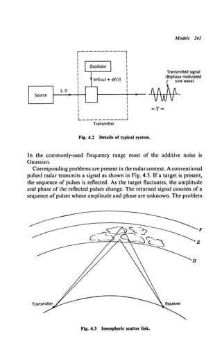
258. 242 4.1 Introduction
- 1me-varymg enve ope
/'
~ :-
___ .....
T'
'"" '
LY-
u -.1.;
''-....
!,...--
_y
(Frequency differences exaggerated)
WO WO Wl
Fig. 4.4 Signal component in time-varying channel.
is to examine this sequence in the presence of receiver noise and decide
whether a target is present.
There are obvious similarities between the two areas, but there are also
some differences :
l. In a digital communication system the two types oferror (say 1, when
0 was sent, and vice versa) are usually of equal importance. Furthermore,
a signal may be present on both hypotheses. This gives a symmetry to the
problem that can be exploited. In a radar/sonar system the two types of
(a)
(b)
Fig. 4.5 Signals in radar model: (a) transmitted sequence of rf pulses; (b) received
sequence [amplified (time-shift not shown)].

259. Models 243
error are almost always of unequal importance. In addition, a signal is
present only on one hypothesis. This means that the problem is generally
nonsymmetric.
2. In a digital communication system the probability of error is usually
an adequate measure of system performance. Normally, in radar/sonar a
reasonably complete ROC is needed.
3. In a digital system we are sending a sequence of digits. Thus we can
correct digit errors by putting some structure into the sequence. In the
radar/sonar case this is not an available alternative.
In spite of these differences, a great many of the basic results will be
useful for both areas.
Estimation. The second problem of interest is the estimation of signal
parameters, which is encountered in both the communications and radar/
sonar areas. We discuss a communication problem first.
Consider the analog message source shown in Fig. 4.6a. For simplicity
we assume that it is a sample function from a bandlimited random process
(2W cps: double-sided). We could then sample it every l/2W seconds
without losing any information. In other words, given these samples at the
Analog
source
Sample
values;
A1, Azoo•
Sample
values;
AJ,A2"'
Pulse
frequency
modulator
(a)
(b)
(c)
Sampler
Fig. 4.6 Analog message transmission.

260. 244 4.1 Introduction
n(t)
a(t)
Fig. 4.7 A parameter transmission system.
receiver, we could reconstruct the message exactly (e.g. Nyquist, [4] or
Problem 3.3.6). Every T seconds (T = l/2W) we transmit a signal that
depends on the particular value A1 at the last sampling time. In the system
in Fig. 4.6b the amplitude of a sinusoid depends on the value of A1• This
system is referred to as a pulse-amplitude modulation system (PAM). In
the system in Fig. 4.6c the frequency of the sinusoid depends on the sample
value. This system is referred to as a pulse frequency modulation system
(PFM). The signal is transmitted over a channel and is corrupted by noise
(Fig. 4.7). The received signal in the ith interval is:
r(t) = s(t, A1) + n(t), (2)
The purpose ofthe receiver is to estimate the values ofthe successive A1 and
use these estimates to reconstruct the message.
A typical radar system is shown in Fig. 4.8. In a conventional pulsed
radar the transmitted signal is a sinusoid with a rectangular envelope.
s1(t) = V2£; sin wet, 0 :s; t :s; T,
= 0, elsewhere. (3a)
Fig. 4.8 Radar system diagram.
Target
•
~locity V1

261. Format 245
The returned signal is delayed by the round-trip time to the target. If the
target is moving, there is Doppler shift. Finally there is a random amplitude
and phase due to the target fluctuation. The received signal in the absence
of noise is
Sr(t) = V V2Et sin ((we + wv)(t - T) + ~{>], T~t~T+T.
= 0, elsewhere. (3b)
Here we estimate T and wv (or, equivalently, target range and velocity).
Once again, there are obvious similarities between the communication and
radar/sonar problem. The basic differences are the following:
l. In the communications context A1 is a random variable with a prob-
ability density that is usually known. In radar the range or velocity limits
of interest are known. The parameters, however, are best treated as non-
random variables (e.g., discussion in Section 2.4).
2. In the radar case the difficulty may be compounded by a lack of
knowledge regarding the target's presence. Thus the detection and esti-
mation problem may have to be combined.
3. In almost all radar problems a phase reference is not available.
Other models of interest will appear naturally in the course of our
discussion.
4.1.2 Format
Because this chapter is long, it is important to understand the over-all
structure. The basic approach has three steps:
1. The observation consists of a waveform r(t). Thus the observation
space may be infinite dimensional. Our first step is to map the received
signal into some convenient decision or estimation space. This will reduce
the problem to one studied in Chapter 2.
2. In the detection problem we then select decision regions and compute
the ROC or Pr (£). In the estimation problem we evaluate the variance or
mean-square error.
3. We examine the results to see what they imply about system design
and performance.
We carry out these steps for a sequence of models of increasing com-
plexity (Fig. 4.9) and develop the detection and estimation problem in
parallel. By emphasizing their parallel nature for the simple cases, we can
save appreciable effort in the more complex cases by considering only one
problem in the text and leaving the other as an exercise. We start with the
simple models and then proceed to the more involved.

262. 246 4.2 Detection and Estimation in White Gaussian Noise
Signal
Channel Signal detection parameter estimation
Additive Simple Single
white binary parameter,
noise linear
Additive General Single
colored binary parameter,
noise nonlinear
Simple M-ary Multiple
random parameter
Multiple
channels
Fig. 4.9 Sequence of models.
A logical question is: if the problem is so simple, why is the chapter so
long? This is a result of our efforts to determine how the model and its
parameters affect the design and performance of the system. We feel that
only by examining some representative problems in detail can we acquire
an appreciation for the implications of the theory.
Before proceeding to the solution, a briefhistorical comment is in order.
The mathematical groundwork for our approach to this problem was
developed by Grenander [5]. The detection problem relating to optimum
radar systems was developed at the M.I.T. Radiation Laboratory, (e.g.,
Lawson and Uhlenbeck [6]) in the early 1940's. Somewhat later Woodward
and Davies [7, 8] approached the radar problem in a different way. The
detection problem was formulated at about the same time in a manner
similar to ours by both Peterson, Birdsall, and Fox [9] and Middleton and
Van Meter [10], whereas the estimation problem was first done by Slepian
[11]. Parallel results with a communications emphasis were developed by
Kotelnikov [12, 13] in Russia. Books that deal almost exclusively with
radar include Helstrom [14] and Wainstein and Zubakov [15]. Books that
deal almost exclusively with communication include Kotelnikov [13],
Harman [16], Baghdady (ed.) [17], Wozencraft and Jacobs [18], and
Golomb et al. [19]. The last two parts of Middleton [47] cover a number of
topics in both areas. By presenting the problems side by side we hope to
emphasize their inherent similarities and contrast their differences.
4.2 DETECTION AND ESTIMATION IN WHITE GAUSSIAN NOISE
In this section we formulate and solve the detection and estimation
problems for the case in which the interference is additive white Gaussian
noise.

263. Detection of Signals in Additive White Gaussian Noise: Simple Binary 247
We consider the detection problem first: the simple binary case, the
general binary case, and the M-ary case are discussed in that order. By
using the concept of a sufficient statistic the optimum receiver structures
are simply derived and the performances for a number of important cases
are evaluated. Finally, we study the sensitivity of the optimum receiver to
the detailed assumptions of our model.
As we have seen in the classical context, the decision and estimation
problems are closely related; linear estimation will turn out to be essentially
the same as simple binary detection. When we proceed to the nonlinear
estimation problem, new issues will develop, both in specifying the
estimator structure and in evaluating its performance.
4.2.1 Detection of Signals in Additive White Gaussian Noise
Simple BiMry Detection. In the simplest binary decision problem the
received signal under one hypothesis consists of a completely known
signal, VE s(t). corrupted by an additive zero-mean white Gaussian noise
w(t) with spectral height N0/2; the received signal under the other hypoth-
esis consists of the noise w(t) alone. Thus
r(t) = VB s(t) + w(t),
= w(t),
For convenience we assume that
0 ~ t ~ T:H1,
0 ~ t ~ T:H0• (4)
(5)
so that E represents the received signal energy. The problem is to observe
r(t) over the interval [0, T] and decide whether H0 or H1 is true. The
criterion may be either Bayes or Neyman-Pearson.
The following ideas will enable us to solve this problem easily:
I. Our observation is a time-continuous random waveform. The first
step is to reduce it to a set of random variables (possibly a countably
infinite set).
2. One method is the series expansion of Chapter 3:
K
r(t) = l.i.m. 2 r1 cf>t(t);
K-oo i=l
O~t~T. (6)
When K = K', there are K' coefficients in the series, r1o ... , rx· which
we could denote by the vector rx·· In our subsequent discussion we suppress
the K' subscript and denote the coefficients by r.

264. 248 4.2 Detection and Estimation in White Gaussian Noise
r(t)
tyVVvv Decomposition r Rotation l Decision
into of
Continuous coordinates Infinite coordinates Sufficient
device
dimensional
waveform
vector statistic
y
Fig. 4.10 Generation of sufficient statistics.
3. In Chapter 2 we saw that if we transformed r into two independent
vectors, I (the sufficient statistic) and y, as shown in Fig. 4.10, our decision
could be based only on I, because the values of y did not depend on the
hypothesis. The advantage ofthis technique was that it reduced the dimen-
sion of the decision space to that of I. Because this is a binary problem
we know that I will be one-dimensional.
Here the method is straightforward. If we choose the first orthonormal
function to be s(t), the first coefficient in the decomposition is the Gaussian
random variable,
{J:s(t) w(t) dt 0. w1 :H0,
r- m
1
- {Ts(t)[VE s(t) + w(t)] dt = VB + w1: H1.
The remaining r1 (i > 1) are Gaussian random variables which can be
generated by using some arbitrary orthonormal set whose members are
orthogonal to s(t).
{
LT r/J1(t) w(t) dt 0. w1:H0 ,
r1 = i =f. 1. (8)
LT rfo1(t)[VE s(t) + w(t)] dt = w1:H1 ,
From Chapter 3 (44) we know that
E(w1w1) = 0; i # j.
Because w1 and w1 are jointly Gaussian, they are statistically independent
(see Property 3 on p. 184).
We see that only r1 depends on which hypothesis is true. Further, all
r1 (i > 1) are statistically independent of r1 • Thus r1 is a sufficient statistic
(r1 = 1). The other r1 correspond to y. Because they will not affect the
decision, there is no need to compute them.

265. Detection of Signals in Additive White Gaussian Noise: Simple Binary 249
r(t)
s(t)
Fig. 4.11 Correlation receiver.
Several equivalent receiver structures follow immediately. The structure
in Fig. 4.11 is called a correlation receiver. It correlates the input r(t) with
a stored replica of the signal s(t). The output is rt. which is a sufficient
statistic (r1 = /) and is a Gaussian random variable. Once we have
obtained rt. the decision problem will be identical to the classical problem
in Chapter 2 (specifically, Example 1 on pp. 27-28). We compare I to a
threshold in order to make a decision.
An equivalent realization is shown in Fig. 4.12. The impulse response
of the linear system is simply the signal reversed in time and shifted,
(9)
The output at time T is the desired statistic /. This receiver is called a
matched filter receiver. (It was first derived by North [20].) The two
structures are mathematically identical; the choice of which structure to
use depends solely on ease of realization.
Just as in Example 1 of Chapter 2, the sufficient statistic I is Gaussian
under either hypothesis. Its mean and variance follow easily:
E(ll H1) = E(r1l H1) = VE,
E(IJ H0) = E(r11H0) = 0,
Var (/I Ho) = Var (/I H1) = ~0•
Thus we can use the results of Chapter 2, (64)-(68), with
r(t)
d= (~f'"·
Observe at time t =Tr-------.
Linear
system t----
h(r)
h(r)=s(T-r), O:'St:'ST,
0 elsewhere.
r1
Fig. 4.12 Matched filter receiver.
(10)
(11)

266. 250 4.2 Detection and Estimation in White Gaussian Noise
t
Fig. 4.13 Receiver operating characteristic: known signal in additive white Gaussian
noise.
The curves in Figs. 2.9a and 2.9b of Chapter 2 are directly applicable and
are reproduced as Figs. 4.13 and 4.14. We see that the performance
depends only on the received signal energy E and the noise spectral height
N0-the signal shape is not important. This is intuitively logical because
the noise is the same along any coordinate.
The key to the simplicity in the solution was our ability to reduce an
infinite dimensional observation space to a one-dimensional decision space
by exploiting the idea of a sufficient statistic. Clearly, we should end up
with the same receiver even if we do not recognize that a sufficient statistic
is available. To demonstrate this we construct the likelihood ratio directly.
Three observations lead us easily to the solution.
1. If we approximate r(t) in terms of some finite set of numbers,

267. Detection ofSignals in Additive White Gaussian Noise: Simple Binary 251
Fig. 4.14 Probability of detection vs {~~)y..
r1o ..., rK, (r), we have a problem in classical detection theory that we can
solve.
2. If we choose the set r1o r2, ••• , rK so that
K
Prl•'2·····'KiH,(Rl> R2, ... , RKIH,) = n PriiH,(R,IH,),
i= 1
i = 0, I, (12)
that is, the observations ~re conditionally independent, we have an easy
problem to solve.

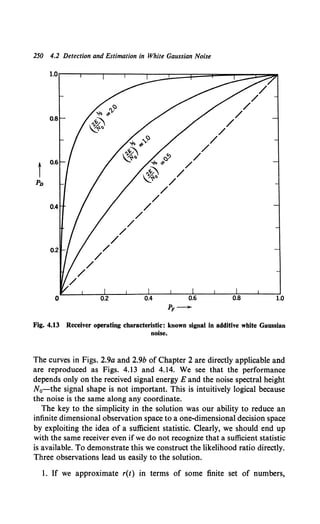
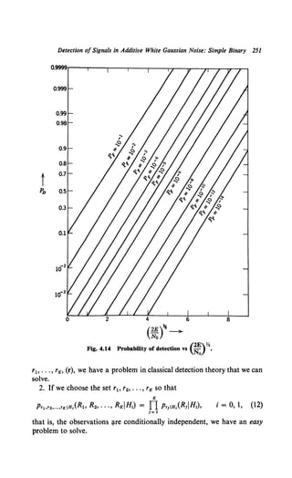
268. 252 4.2 Detection and Estimation in White Gaussian Noise
3. Because we know that it requires an infinite set of numbers to
represent r(t) completely, we want to get the solution in a convenient form
so that we can let K--+ oo.
We denote the approximation that uses K coefficients as rK(t). Thus
K
rK(t) = L r1 (Mt), 0 :5: t :5: T, (13)
1=1
where
r1= S:r(t) (Mt) dt, i = 1,2, .. .K, (14)
and the (Mt) belong to an arbitrary complete orthonormal set offunctions.
Using (14), we see that under H0
r1= S: w(t) cMt) dt = w" (15)
and under H1
r1 = LT VEs(t) cMt) dt + J: w(t) cMt) dt = s1 + w1• (16)
The coefficients s1 correspond to an expansion of the signal
K
sK(t) Q L S1 cPt(t), 0 :5: t :5: T,
1=1
and
v'E s(t) = lim sK(t).
K-+a>
The rt's are Gaussian with known statistics:
E(rtiHo) = 0,
E(r1iH1) = s"
Var (r1IH0) = Var (rtiH1) = ~0•
(17)
(18)
(19)
Because the noise is "white," these coefficients are independent along any
set of coordinates. The likelihood ratio is
Il
K 1 ( 1 (R1 - s1) 2)
- - exp -- .:.....:':-;-="-
A[ ( )] - PriH• (Ri Hl) - I= 1 V~ 2 No/2 (20)
rK t - PriHo(RIHo) - ITK 1 ( I Rl2 ) •
--exp ----
t=l V7TNo 2 No/2
Taking the logarithm and canceling common terms, we have
2 K } K
In A[rK(t)] = Jr 2 R1s, - N, 2 s12• (21)
HOI=l 01=1

269. Detection of Signals in Additive White Gaussian Noise: Simple Binary 253
The two sums are easily expressed as integrals. From Parseval's theorem,
and
(22)
We now have the log likelihood ratio in a form in which it is convenient
to pass to the limit:
. 2v1fiT E
l.I.m. In A[rK(t)] Q ln A[r(t)] = u r(t) s(t) dt - ,.7 •
K-+o> Ho O Ho
(23)
The first term is just the sufficient statistic we obtained before. The
second term is a bias. The resulting likelihood ratio test is
2vEiT Hl E
N r(t) s(t) dt ~ ln 7J + N ·
o o Ho o
(24)
(Recall from Chapter 2 that 7J is a constant which depends on the costs
and a priori probabilities in a Bayes test and the desired PF in a Neyman-
Pearson test.) It is important to observe that even though the probability
density Pr<tliH,(r(t)IH1) is not well defined for either hypothesis, the likeli-
hood ratio is.
Before going on to more general problems it is important to emphasize
the two separate features of the signal detection problem:
I. First we reduce the received waveform to a single number which is a
point in a decision space. This operation is performed physically by a
correlation operation and is invariant to the decision criterion that we
plan to use. This invariance is important because it enables us to construct
the waveform processor without committing ourselves to a particular
criterion.
2. Once we have transformed the received waveform into the decision
space we have only the essential features of the problem left to consider.
Once we get to the decision space the problem is the same as that studied
in Chapter 2. The actual received waveform is no longer important and
all physical situations that lead to the same picture in a decision space are
identical for our purposes. In our simple example we saw that all signals
of equal energy map into the same point in the decision space. It is
therefore obvious that the signal shape is unimportant.
The separation of these two parts of the problem leads to a clearer
understanding of the fundamental issues.

270. 254 4.2 Detection and Estimation in White Gaussian Noise
General Binary Detection in White Gaussian Noise. The results for the
simple binary problem extend easily to the general binary problem. Let
r(t) = VB;_ s1(t) + w(t),
= VE0 s0(t) + w(t),
0::;;; t::;;; T:Ht.
0::;;; t::;;; T:H0, (25)
where s0(t) and s1(t) are normalized but are not necessarily orthogonal.
We denote the correlation between the two signals as
p Q J:s0(t) s1(t) dt.
(Note that !PI ::;;; 1 because the signals are normalized.)
We choose our first two orthogonal functions as follows:
l/>1(t) = s1(t), 0 ::;;; t ::;;; T, (26)
0::;;; t::;;; T. (27)
We see that l/>2(t) is obtained by subtracting out the component of s0(t)
that is correlated with if>1(t) and normalizing the result. The remaining
if>1
(t) consist ofan arbitrary orthonormal set whose members are orthogonal
to if>1(t) and if>2(t) and are chosen so that the entire set is complete. The
coefficients are
i = 1, 2, .... (28)
All of the r1 except r1 and r2 do not depend on which hypothesis is true
and are statistically independent of r1 and r2• Thus a two-dimensional
decision region, shown in Fig. 4.15a, is adequate. The mean value of r1
along each coordinate is
E[rt!Ho] = flo s:s0(t) !/>1(t) dt, !d Sob i = 1, 2, :H0 , (29)
and
i = 1, 2, :H1• (30)
The likelihood ratio test follows directly from Section 2.6 (2.327)
1 2 } 2 Ht
In A = -No ,6(R, - s11) 2 + No ,6(~ -s01) 2 ~In 7J, (3la)
1 I Ht
InA= --IR- s1l2 + -IR- sol2 ~ ln7J, (3lb)
No No Ho
or, canceling common terms and rearranging the result,
Ht N. l
R.T(sl - So)~ 2°1n 7J + 2(js1!2 - lsol2). (31c)

271. Detection of Signals in Additive White Gaussian Noise: General Binary 255
(a)
f r2
I
I
I
I
I
I
(b)
SayHo
Fig. 4.15 Decision spaces.
Decision line
Say H1
y
Thus only the product of RT with the difference vector s1 - s0 is used to
make a decision. Therefore the decision space is divided into two parts by
a line perpendicular to s1 -- s0 as shown in Fig. 4.15b. The noise com-
ponents along the r1 and r2 axes are independent and identically distributed.
Now observe that we can transform the coordinates as shown in Fig.
4.15b. The noises along the new coordinates are still independent, but only
the coefficient along the I coordinate depends on the hypothesis and the y
coefficient may be disregarded. Therefore we can simplify our receiver by

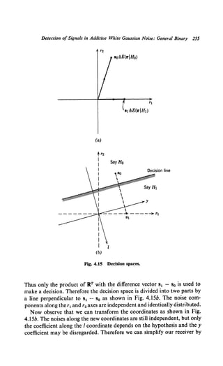
272. 256 4.2 Detection and Estimation in White Gaussian Noise
generating I instead of r1 and r2• The function needed to generate the
statistic is just the normalized version of the difference signal. Denote
the difference signal by s,..(t):
s,..(t) Q VE1 s1(t) - VE0 s0(t). (32)
The normalized function is
I' () _ VE1 s1(t)- VE0 s0(t)
Jt.t - •
(E1 - 2pVE0 E1 + Eo)Y.
(33)
The receiver is shown in Fig. 4.16. (Note that this result could have been
obtained directly by choosingf,..(t) as the first orthonormal function.)
Thus once again the binary problem reduces to a one-dimensional
decision space. The statistic I is Gaussian:
E(lJHl) = El - vE;E;_ P '
(E1 - 2pVE;E;_ + E0)Y•
(34)
E(IJHo) = yE;ff;_ P - Eo .
(E1 - 2pVE;;E;_ + E0 )Y.
(35)
The variance is N0 /2 as before. Thus
(36)
Observe that if we normalized our coordinate system so that noise variance
was unity then d would be the distance between the two signals. The
resulting probabilities are
(ln 17 d)
PF = erfc* d + 2 •
(ln 11 d)
Pv = erfc* d - 2 ·
[These equations are just (2.67) and (2.68).]
r(t)
·rt-------~[E~----;o
..../E;s1(t)- -./Eoso(t)
f,..(t)= (E!-2P~+Eo)~
Fig. 4.16 Optimum correlation receiver, general binary problem.
(37)
(38)

273. Detection of Signals in Additive White Gaussian Noise: M-ary Detection 257
The best choice of signals follows easily. The performance index dis
monotonically related to the distance between the two signals in the
decision space. For fixed energies the best performance is obtained by
making p = - 1. In other words,
(39)
Once again the signal shape is not important.
When the criterion is minimum probability of error (as would be the
logical choice in a binary communication system) and the a priori prob-
abilities of the two hypotheses are equal, the decision region boundary has
a simple interpretation. It is the perpendicular bisector of the line con-
necting the signal points (Fig. 4.17). Thus the receiver under these circum-
stances can be interpreted as a minimum-distance receiver and the error
probability is
Pr (fi) = J"' -1- exp {-x2
) dx = erfc* {~)· (40)
d/2 vT,; 2 2
If, in addition, the signals have equal energy, the bisector goes through the
origin and we are simply choosing the signal that is most correlated with
r(t). This can be referred to as a "largest-of" receiver (Fig. 4.18).
The discussion can be extended to the M-ary problem in a straight-
forward manner.
M-ary Detection in White Gaussian
M-hypotheses:
r(t) = V£1 s1(t) + w(t);
Noise. Assume that there are
Minimum probability
of error decision
line
(41)
Fig. 4.17 Decision space.

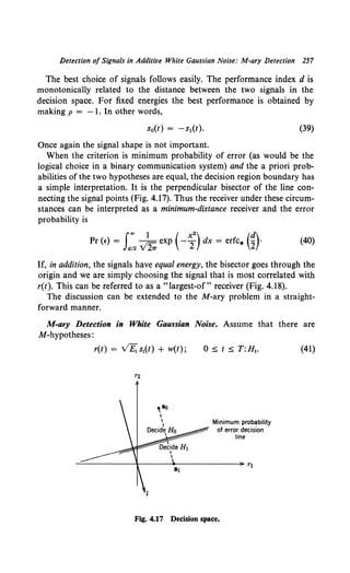
274. 258 4.2 Detection and Estimation in White Gaussian Noise
r(t)
so(t)
Fig. 4.18 "Largest of" receiver.
The s1(t) all have unit energy but may be correlated:
JoT s1
(t) s1(t) dt = p11• i,j = 1, 2, ... , M. (42)
This problem is analogous to theM-hypothesis problem in Chapter 2.
We saw that the main difficulty for a likelihood ratio test with arbitrary
costs was the specification of the boundaries of the decision regions. We
shall devote our efforts to finding a suitable set of sufficient statistics and
evaluating the minimum probability of error for some interesting cases.
First we construct a suitable coordinate system to find a decision space
with the minimum possible dimensionality. The procedure is a simple
extension of the method used for two dimensions. The first coordinate
function is just the first signal. The second coordinate function is that
component of the second signal which is linearly independent of the first
and so on. We let
cP1(t) = s1(t),
cP2(t) = (1 - P122)-%[s2(t) - P12 s1(t)].
To construct the third coordinate function we write
cPa(t) = Ca[sa(t) - C1cP1(t) - C2cP2(t)],
(43a)
(43b)
(43c)
and find c1 and c2 by requiring orthogonality and c3 by requiring rPa(t) to
be normalized. (This is called the Gram-Schmidt procedure and is
developed in detail in Problem 4.2.7.) We proceed until one of two things
happens:
1. M orthonormal functions are obtained.
2. N ( < M) orthonormal functions are obtained and the remaining
signals can be represented by linear combinations of these orthonormal
functions. Thus the decision space will consist of at most M dimensions
and fewer if the signals are linearly dependent.t
t Observe that we are talking about algebraic dependence.

275. Detection ofSignals in Additive White Gaussian Noise: M-ary Detection 259
We then use this set of orthonormal functions to generate N coefficients
(N ~ M)
rl ~ rr(t) tPt(t) dt, i = I, 2, ... , N. (44a)
These are statistically independent Gaussian random variables with
variance N0 (2 whose means depend on which hypothesis is true.
E[rdH1] ~ mli, i = 1, ... , N, (44b)
j = 1, ... ,M.
The likelihood ratio test follows directly from our results in Chapter 2
(Problem No. 2.6.1). When the criterion is minimum Pr (~:),we compute
1 N
It = In pi - N L (Rt - mti)2,
0 I =1
j= 1, ... ,M, (45)
and choose the largest. (The modification for other cost assignments is
given in Problem No. 2.3.2.)
Two examples illustrate these ideas.
Example 1. Let
St{t) = (~f' sin [Wet + (i- 1) n
and
21Tn
We=T
i = I, 2, 3, 4,
(n is an arbitrary integer). We see that
</>I(t) = (-ftsin wet,
and
(2)%
</>2(t) = T COS Wet,
OStST, i = 1, 2, 3, 4,
(46)
OStST,
(47)
OstsT.
We see s3 (t) and s4(t) are - </>1 (1) and - </>2(1) respectively. Thus, in this case,
M = 4 and N = 2. The decision space is shown in Fig. 4.19a. The decision regions
follow easily when the criterion is minimum probability of error and the a priori
probabilities are equal. Using the result in (45), we obtain the decision regions in
Fig. 4.19b.
Example 2. Let
OStST,
OStST, (48)
(2)% 61rn
s3(t) = T sin T t, OStST,
(n is an arbitrary integer) and
i = 1, 2, 3.
Now
(49)

276. 260 4.2 Detection and Estimation in White Gaussian Noise
sa
(a) (b)
Fig. 4.19 Decision space.
In this case, M = N = 3 and the decision space is three-dimensional, as shown in
Fig. 4.20a. For min Pr (•) and equal a priori probabilities the decision regions follow
easily from (45). The boundaries are planes perpendicular to the plane through s1, s2 ,
and S3. Thus it is only the projection of R on this plane that is used to make a decision,
and we can reduce the decision space to two dimensions as shown in Fig. 4.20b.
(The coefficients r~ and r~ are along the two orthonormal coordinate functions used
to define the plane.)
Note that in Examples 1 and 2 the signal sets were so simple that the
Gram-Schmidt procedure was not needed.
It is clear that these results are directly analogous to the M hypothesis
case in Chapter 2. As we have already seen, the calculation of the errors is
conceptually simple but usually tedious for M > 2. To illustrate the
procedure, we compute the Pr (~;-) for Example 1.
ra Ha
(a) (b)
Fig. 4.20 Decision space: orthogonal signals.

277. Detection ofSignals in Additive White Gaussian Noise: M-ary Detection 261
Example I (continued). We assume that the hypotheses are equally likely. Now the
problem is symmetrical. Thus it is sufficient to assume that s1(t) was transmitted and
compute the resulting Pr (£). (Clearly, Pr (£) = Pr (£1H,), i = 1, ... , 4.) We also
observe that the answer would be invariant to a 45° rotation of the signal set
because the noise is circularly symmetric.
Thus the problem of interest reduces to the simple diagram shown in Fig. 4.21.
The Pr (£)is simply the probability that r lies outside the first quadrant when H1is
true.
Now r1 and r2 are independent Gaussian variables with identical means and
variances:
and
E(rdH1) = E(r2IH1) = (~) y,
Var (r1IH1) = Var (r2IH1) = ~0• (50)
The Pr (£) can be obtained by integrating p,1.,21u1(R~> R2IH1) over the area outside
the first quadrant. Equivalently, Pr (•) is the integral over the first quadrant subtracted
from unity.
Pr (£) = 1- [[ (2w~o) -l> exp (- (R1 - ;:Efi.)2
) dR1 r (51)
Changing variables, we have
Pr (£) = 1 - (fvE/No .}2wexp (- ;) dx)" = 1 - (erfc* [- (:orJf. (52)
which is the desired result.
Another example of interest is a generalization of Example 2.
Example 3. Let us assume that
r(t) = VE s1(t) + w(t),
and
OstsT,
P11 = &v
i = I, 2, ..., M (53)
(54)
and the hypotheses are equally likely. Because the energies are equal, it is convenient to
First quadrant corresponds
to correct decision when
H1 is true
si
Fig. 4.21 Rotation of signal.

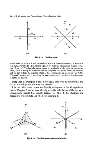
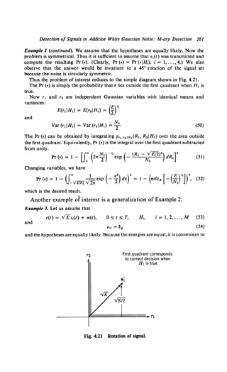
278. 262 4.2 Detection and Estimation in White Gaussian Noise
implement the LRT as a "greatest of" receiver as shown in Fig. 4.22. Once again the
problem is symmetric, so we may assume H, is true. Then an error occurs if any
1
1 > /, : j oF 1, where
l1 ~ J:r(t)s1(t) dt, j = 1, 2, ... , M.
Thus
Pr (•) = Pr (EIH,) = I - Pr (all/1 < I, : j oF liH,) (55)
or, noting that the 1
1 (j '#- 1) have the same density on H,,
(56)
In this particular case the densities are
(57)
and
j '#- l. (58)
Substituting these densities into (56) and normalizing the variables, we obtain
f., 1 { (x-(2£/N0
)Y•)2
}(J" 1 [ y2
] )M-1
Pr(E)= 1- _.,dx.y2.,.exp - 2 _.,.y2.,.exp -2 dy
(59)
Unfortunately, we cannot integrate this analytically. Numerical results for certain
r(t)
Fig. 4.22 "Largest of" receiver.

279. Detection ofSig1Ulls in Additive White Gaussian Noise: M-ary Detection 26J
t
Pr(e)
E/No-
Fig. 4.23 Error probabiUty: M orthogonal signals.
values of M and E/No are tabulated in [21 I and shown in Fig. 4.23. For some of our
purposes an approximate analytic expression is more interesting. We derive a very
simple bound. Some other useful bounds are derived in the problems. Looking at (55),
we see that we could rewrite the Pr (~)as
Pr <~> = Pr (any 1
1> /1 :j '# 1 IH1),
Pr (E) = Pr U2 > /1 or /3 > h or
(60)
(61)

280. 264 4.2 Detection and Estimation in White Gaussian Noise
Now, several /1 can be greater than ft. (The events are not mutually exclusive.) Thus
Pr (e) :s; Pr (/2 > It) + Pr (/a > h) + ···+ Pr (IM > It), (62)
Pr (e) :s; (M- 1){f., ) 2.. exp [-(x- v'~)2]({• )
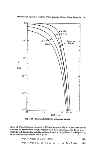
2.. exp ( -~) dy)dx};
(63)
but the term in the bracket is just the expression of the probability of error for two
orthogonal signals. Using (36) with p = 0 and E1 = Eo = E in (40), we have
Pr (e) :s; (M- 1) J"'_v'1 exp (-L
2
2
) dy.
..!E/No 2?T
(64)
(Equation 64 also follows directly from (63) by a change of variables.) We can further
simplify this equation by using (2.71):
< (M- 1) ( E)
Pr (e) _ v' v' exp - 2N ·
2w EfN0 o
(65)
We observe that the upper bound increases linearly with M. The bound on the Pr (e)
given by this expression is plotted in Fig. 4.23 for M = 16.
A related problem in which M orthogonal signals arise is that of
transmitting a sequence of binary digits.
Example 4. Sequence ofDigits. Consider the simple digital system shown in Fig. 4.24,
in which the source puts out a binary digit every T seconds. The outputs 0 and 1 are
equally likely. The available transmitter power is P. For simplicity we assume that
we are using orthogonal signals. The following choices are available:
1. Transmit one of two orthogonal signals every T seconds. The energy per signal
is PT.
2. Transmit one of four orthogonal signals every 2Tseconds. The energy per signal
is 2PT. For example, the encoder could use the mapping,
00 ..... so(t)
1,0,0,1 01-st(t)
10...., s2(t)
u-sa(t)
Encoder
00-->- So(t ),
01 -->- SI(t),
10-->- s.(t),
11 -->- sa(t).
s;(t)
signal every
2Tsec
r2T
Jo Si(t) sj(t) dt = Oij
n(t)
Fig. 4.24 Digital communication system.

281. Detection of Signals in Additive White Gaussian Noise: M-ary Detection 265
3. In general, we could transmit one of M orthogonal signals every T log2 M
seconds. The energy per signal is TP!og. M. To compute the probability of error we
use (59):
f., 1 { 1[ (2PTlog M)ll]"}
Pr(E) = 1- _., dx v'2.,. exp - 2 x- No 2
[fx 1 ( y2) ]M-1
x ~exp -- dy · (66)
_.,. v'z.,. 2
The results have been calculated numerically [19] and are plotted in Fig. 4.25. The
behavior is quite interesting. Above a certain value of PT/No the error probability
decreases with increased M. Below this value the converse is true. It is instructive to
investigate the behavior as M -~ oo. We obtain from (66), by a simple change of
variables,
f., e-•2
12 { M- 1 [ (2PT!o M)y,]}
lim (1- Pr(E)) = dy • 1_ lim erf* y + N,g. ·
M-+ao -co ·v27T M...,ao o
(67)
Now consider the limit of the logarithm of the expression in the brace:
. In erf* [y + (2PT~g• ~r1
J~~ (M- 1)-1 . (68)
Evaluating the limit by treating Mas a continuous variable and using L'Hospital's
rule, we find that (see Problem 4.2.15)
{
-00
lim In{-}= '
M-"'
0,
PT
No< In 2,
PT
No >In 2.
(69)
Thus, from the continuity of logarithm,
{
0,
lim Pr (E) =
M_.,
1,
PT
No >In 2,
(70)
PT
No <In 2.
Thus we see that there is a definite threshold effect. The value of Tis determined by
how fast the source produces digits. Specifically, the rate in binary digits per second is
R ~ fbinary digits/sec.
Using orthogonal signals, we see that if
1 p
R < ln2N0
(71)
(72)
the probability of error will go to zero. The obvious disadvantage is the bandwidth
requirement. As M---+ oo, the transmitted bandwidth goes to oo.
The result in (72) was derived for a particular set of signals. Shannon
has shown (e.g., [22] or [23]) that the right-hand side is the bound on the

282. 1
t
Pr(E)
2 3 4 5 6 7
PT/No-
Fig. 4.25 Probability of decision error: M orthogonal signals, power constraint.
266

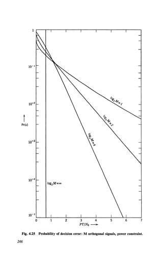
283. Detection of Signals in Additive White Gaussian Noise: Sensitivity 267
rate for error-free transmission for any communication scheme. This rate
is referred to as the capacity of an infinite bandwidth, additive white
Gaussian noise channel,
Coo = 1~2 ~0 bits/sec. (73)
Shannon has also derived an expression for a bandlimited channel
(Wch: single-sided}:
(74)
These capacity expressions are fundamental to the problem of sending
sequences of digits. We shall not consider this problem, for an adequate
discussion would take us too far afield. Suitable references are [18] and [66].
In this section we have derived the canonic receiver structures for the
M-ary hypothesis problem in which the received signal under each hypoth-
esis is a known signal plus additive white Gaussian noise. The simplicity
resulted because we were always able to reduce an infinite dimensional
observation space to a finite ( ~ M) dimensional decision space.
In the problems we consider some of the implications of these results.
Specific results derived in the problems include the following:
1. The probability of error for any set of M equally correlated signals
can be expressed in terms of an equivalent set of M orthogonal signals
(Problem 4.2.9).
2. The lowest value of uniform correlation is -(M- 1)-1• Signals
with this property are optimum when there is no bandwidth restriction
(Problems 4.2.9-4.2.12). They are referred to as Simplex signals.
3. For large M, orthogonal signals are essentially optimum.
Sensitivity. Before leaving the problem of detection in the presence of
white noise we shall discuss an important issue that is frequently over-
looked. We have been studying the mathematical model of a physical
system and have assumed that we know the quantities of interest such as
s(t), E, and N0 exactly. In an actual system these quantities will vary from
their nominal values. It is important to determine how the performance of
the optimum receiver will vary when the nominal values are perturbed. If
the performance is highly sensitive to small perturbations, the validity of
the nominal performance calculation is questionable. We shall discuss
sensitivity in the context of the simple binary detection problem.
The model for this problem is
r(t) = VE s(t) + w(t),
r(t) = w(t),
0 ~ t ~ T:H1
0 ~ t ~ T:Ho. (75)

284. 268 4.2 Detection and Estimation in White Gaussian Noise
The receiver consists ofa matched filter followed by a decision device. The
impulse response of the matched filter depends on the shape of s(t).
The energy and noise levels affect the decision level in the general Bayes
case. (In the Neyman-Pearson case only the noise level affects the threshold
setting). There are several possible sensitivity analyses. Two of these are
the following:
I. Assume that the actual signal energy and signal shape are identical
to those in the model. Calculate the change in Pv and PF due to a change
in the white noise level.
2. Assume that the signal energy and the noise level are identical to
those in the model. Calculate the change in Pv and PF due to a change in
the signal.
In both cases we can approach the problem by first finding the change
in d due to the changes in the model and then seeing how Pv and PF are
affected by a change in d. In this section we shall investigate the effect of
an inaccurate knowledge of signal shape on the value of d. The other
questions mentioned above are left as an exercise. We assume that we have
designed a filter that is matched to the assumed signal s(t),
h(T - t) = s(t), O~t~T. (76)
and that the received waveform on H 1 is
r(t) = sa(t) + w(t), O~t~T. (77)
where sa(t) is the actual signal received. There are two general methods of
relating sa(t) to s(t). We call the first the function-variation method.
Function- Variation Method. Let
sa(t) = VEs(t) + VE, s,(t), O~t~T. (78)
where s,(t) is a normalized waveform representing the inaccuracy. The
energy in the error signal is constrained to equal E,.
The effect can be most easily studied by examining the decision space
(more precisely an augmented decision space). To include all of s,(t) in
the decision space we think of adding another matched filter,
h2(T- t) = cp2(t) = s,(t) - p, s(t),
VI - p,2
O~t~T. (79)
where p, is the correlation between s,(t) and s(t). (Observe that we do not
do this physically.) We now have a two-dimensional space. The effect of
the constraint is clear. Any sa(t) will lead to a point on the circle surround-
ing s, as shown in Fig. 4.26. Observe that the decision still uses only the

285. Detection ofSignals in Additive White Gaussian Noise: Sensitivity 269
Q)
~
c:
0
"iii
~
/--.......
cbt(t)-vs(t)
Fig. 4.26 Signal locus: fixed energy in error signal.
coordinate along s(t). The effect is obvious. The error signal that causes
the largest performance degradation is
s.(t) = -s(t).
Then
To state the result another way,
where
!l.d v~
d =- V2E/N0
fl.d ~da-d.
(80)
(81)
(82)
(83)
We see that small energy in the error signal implies a small change in
performance. Thus the test is insensitive to small perturbations. The
second method is called the parameter-variation method.
Parameter-Variation Method. This method can best be explained by an
example. Let
(2)%
s(t) = T sin wet, O~t~T, (84)
be the nominal signal. The actual signal is
Sa(t) = (¥fsin (wet+ 0), O~t~T, (85)
which, for (} =. 0, corresponds to the nominal signal. The augmented

286. 270 4.2 Detection and Estimation in White Gaussian Noise
Gl
~
c
.!2
Ill
"2
c
''
I
I
----l""-----JI!,..----1/~-v'E-=E=----~ cbi(t)
I
I
I
I
I
/
I
Fig. 4.27 Signal locus: fixed energy in total signal.
decision space is shown in Fig. 4.27. The vector corresponding to the
actual signal moves on a circle around the origin.
(2£)%
da = No COS 8 (86)
and
i).d
d = - (1 - cos 0). (87)
Once again we see that the test is insensitive to small perturbations.
The general conclusion that we can infer from these two methods is
that the results of detection in the presence of white noise are insensitive
to the detailed assumptions. In other words, small perturbations from the
design assumptions lead to small perturbations in performance. In almost
all cases this type of insensitivity is necessary if the mathematical model is
going to predict the actual system performance accurately.
Many statistical analyses tend to ignore this issue. The underlying
reason is probably psychological. After we have gone through an involved
mathematical optimization, it would be pleasant to demonstrate an order-
of-magnitude improvement over the system designed by using an intuitive
approach. Unfortunately, this does not always happen. When it does, we
must determine whether the mathematical result is sensitive to some

287. Linear Estimation 271
detailed assumption. In the sequel we shall encounter several examples of
this sensitivity.
We now turn to the problem of linear estimation.
4.2.2 Linear Estimation
In Section 4.1.1 we formulated the problem of estimating signal param-
eters in the presence of additive noise. For the case of additive white noise
the received waveform is
r(t) = s(t, A) + w(t), O~t~T, (88a)
where w(t) is a sample function from a white Gaussian noise process with
spectral height N0 f2. The parameter A is the quantity we wish to estimate.
If it is a random parameter we will assume that the a priori density is
known and use a Bayes estimation procedure. If it is a nonrandom variable
we will use ML estimates. The function s(t, A) is a deterministic mapping
of A into a time function. If s(t, A) is a linear mapping (in other words,
superposition holds), we refer to the system using the signal as a linear
signaling (or linear modulation) system. Furthermore, for the criterion of
interest the estimator will turn out to be linear so we refer to the problem
as a linear estimation problem. In this section we study linear estimation
and in Section 4.2.3, nonlinear estimation. For linear modulation (88a)
can always be written as
r(t) = AVEs(t) + w(t), O~t~T, (88b)
where s(t) has unit energy.
We can solve the linear estimation problem easily by exploiting its
similarity to the detection problem that we just solved. From Section 2.4
we know that the likelihood function is needed. We recall, however, that
the problem is greatly simplified if we can find a sufficient statistic and
work with it instead of the received waveform. If we compare (88b) and
(4)-(7), it is clear that a sufficient statistic is r1o where
r1 = J:r(t) s(t) dt. (89)
Just as in Section 4.2.1, the probability density of r1o given a = A, is
Gaussian:
E(r1IA) = AVE,
Var (r1 IA) = ~0•
(90)
It is easy to verify that the coefficients along the other orthogonal functions

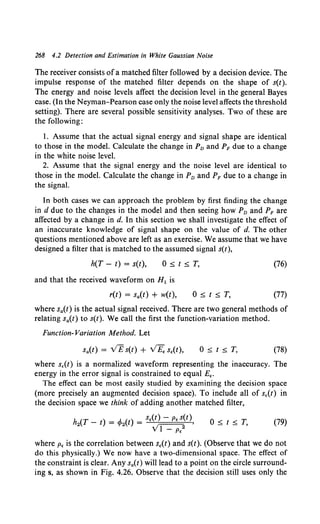
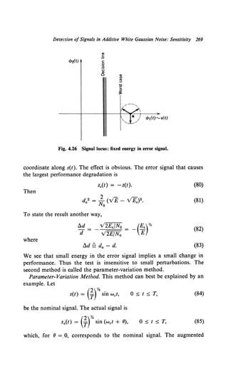
288. 272 4.2 Detection and Estimation in White Gaussian Noise
[see (8)] are independent of a. Thus the waveform problem reduces to the
classical estimation problem (see pp. 58-59).
The logarithm of the likelihood function is
/(A)= _! (R1 -AVE)2
•
2 N 0/2
(91)
If A is a nonrandom variable, the ML estimate is the value of A at which
this function is a maximum. Thus
(92)
The receiver is shown in Fig. 4.28a. We see the estimate is unbiased.
If a is a random variable with a probability density Pa(A), then the
MAP estimate is the value of A where
{93)
is a maximum. For the special case in which a is Gaussian, N(O, aa). the
r(t)
Rt
(a)
Rt
~---~--+------------------
s(t)
2-../E/No
R1 2E/No + 1/ua2
(b)
Fig. 4.28 Optimum receiver, linear estimation: (a) ML receiver;
(b) MAP receiver.

289. Nonlinear Estimation 273
MAP estimate is easily obtained by differentiating lp(A) and equating the
result to zero:
(94)
and
A ( ) 2E/N0 R1
amap Rl = 2EfNo + lfua2 v£" (95)
In both the ML and MAP cases it is easy to show that the result is the
absolute maximum.
The MAP receiver is shown in Fig. 4.28b. Observe that the only differ-
ence between the two receivers is a gain. The normalized error variances
follow easily: for MAP
(MAP). (96)
The quantity aa2E is the expected value of the received energy. For ML
2 6. Ua•2 = (2A2£)-1
ua.n- A2 No (ML). (97)
Here A2E is the actual value ofthe received energy. We see that the variance
ofthe maximum likelihood estimate is the reciprocal ofd2 , the performance
index of the simple binary problem. In both cases we see that the only
way to decrease the mean-square error is to increase the energy-to-noise
ratio. In many situations the available energy-to-noise ratio is not adequate
to provide the desired accuracy. In these situations we try a nonlinear
signaling scheme in an effort to achieve the desired accuracy. In the next
section we discuss the nonlinear estimation.
Before leaving linear estimation, we should point out that the MAP
estimate is also the Bayes estimate for a large class of criteria. Whenever a
is Gaussian the a posteriori density is Gaussian and Properties 1 and 2 on
pp. 60-61 are applicable. This invariance to criterion depends directly on
the linear signaling model.
4.2.3 Nonlinear Estimation
The system in Fig. 4.7 illustrates a typical nonlinear estimation problem.
The received signal is
r(t) = s(t, A) + w(t), 0::;; t::;; T. (98)
From our results in the classical case we know that a sufficient statistic
does not exist in general. As before, we can construct the likelihood

290. 274 4.2 Detection and Estimation in White Gaussian Noise
function. We approach the problem by making a K-coefficient approxima-
tion to r(t). By proceeding as on p. 252 with obvious notation we have
A[ ( ) ] ( I ) Il
K 1 ( 1 [R1 - s1(A)]2 )
rK t 'A = Prla R A = . • ; - exp -2 N /2 .
•=1 v TTN0 o
(99)
where
s1(A) ~ LT s(t, A) cp1(t) dt.
Now, if we let K-+ oo, A[rK(t), A] is not well defined. We recall from
Chapter 2 that we can divide a likelihood function by anything that does
not depend on A and still have a likelihood function. On p. 252 we avoided
the convergence problem by dividing by
K 1 ( 1 R1
2)
PrK(t)IHo [rK(t)JHo] = TI .;-exp -2 N /2 '
1=1 V TTN0 o
before letting K-+ oo. Because this function does not depend on A, it is
legitimate to divide by it here. Define
A1[rK(t) A] = A[rK(t), A] .
' PrK<t>IH0 [rK(t)JHo]
(100)
Substituting into this expression, canceling common terms, letting
K-+ oo, and taking the logarithm we obtain
2 rT 1 rT
In A1 [r(t), A] = No Jo r(t) s(t, A) dt - No Jo s2(t, A) dt. (101)
To find Omz we must find the absolute maximum of this function. To
find dmap we add lnpa(A) to (101) and find the absolute maximum. The
basic operation on the received data consists of generating the first term
in (101) as a function of A. The physical device that we actually use to
accomplish it will depend on the functional form of s(t, A). We shall
consider some specific cases and find the actual structure.
Before doing so we shall derive a result for the general case that will be
useful in the sequel. Observe that if the maximum is interior and ln A1(A)
is differentiable at the maximum, then a necessary, but not sufficient,
condition is obtained by first differentiating (101):
oIn A1(A) =l_ (T [ ( ) _ ( A)] os(t, A) d
oA No Jo r t s t, oA t (102)
(assuming that s(t, A) is differentiable with respect to A). For Omz. a
necessary condition is obtained by setting the right-hand side of (102)
equal to zero. For Omap we add dIn Pa(A)fdA to the right-hand side of (102)

291. Nonlinear Estimation 275
and set the sum equal to zero. In the special case in which Pa(A) is Gaussian,
N(O, ua), we obtain
A 2ua2 fT[() ( A)]os(t,A)dl
amap = No Jo r t - s t, oA t A=dmap• (103)
In the linear case (103) reduces to (95) and gives a unique solution. A
number of solutions may exist in the nonlinear case and we must examine
the sum of (101) and lnp0 (A) to guarantee an absolute maximum.
However, just as in Chapter 2, (102) enables us to find a bound on the
variance of any unbiased estimate of a nonrandom variable and the
addition of d2 In p"(A)/dA2 leads to a bound on the mean-square error in
estimating a random variable. For nonrandom variables we differentiate
(102) and take the expectation
E[021~~1(A)] = ; 0
{ E J:[r(t) - s(t, A)] 02~~/) dt
- E J: [as~~/)f dt}. (104)
where we assume the derivatives exist. In the first term we observe that
E[r(t) - s(t, A)] = E[w(t)] = 0. (105)
In the second term there are no random quantities; therefore the expecta-
tion operation gives the integral itself.
Substituting into (2.179), we have
Var (d- A) ;, 2 J: ["~:A)rdt
(106)
for any unbiased estimate d. Equality holds in (106) if and only if
oIn Al(A) = k(A){d[r(t)] - A} (107)
oA
for all A and r(t). Comparing (102) and (107), we see that this will hold
only for linear modulation. Then dm1 is the minimum variance estimate.
Similarly, for random variables
E[ A - ]2 (E {.3.. rT [os(t, A)]2d - d2lnpa(A)})-l (108)
a a :2: a NoJo oA t dA2 '
where Ea denotes an expectation over the random variable a. Defining
2 /:::,. E rT [os(t, A)]2 dt (109)
i'a - a Jo oA '
we have
D(A _ )2 (.3.. 2 _ E [d2lnpa(A)] )-l
L' a a :2: No i'a a dA2 (110)

292. 276 4.2 Detection and Estimation in White Gaussian Noise
Equality will hold if and only if (see 2.226)
o2 ln A1(A) d2 ln Pa(A)
oA2 + dA2 = constant. (111)
Just as in Chapter 2 (p. 73), in order for (111) to hold it is necessary
and sufficient that Palr<t>[A lr(t) : 0 s t s T] be a Gaussian probability
density. This requires a linear signaling scheme and a Gaussian a priori
density.
What is the value of the bound if it is satisfied only for linear signaling
schemes?
As in the classical case, it has two principal uses:
1. It always provides a lower bound.
2. In many cases, the actual variance (or mean-square error) in a non-
linear signaling scheme will approach this bound under certain conditions.
These cases are the analogs to the asymptotically efficient estimates in the
classical problem. We shall see that they correspond to large E/N0 values.
To illustrate some of the concepts in the nonlinear case we consider two
simple examples.
Example 1. Let s(t) be the pulse shown in Fig. 4.29a. The parameter a is the arrival
-T
{l+cos~t
s(t) =
0
~1(-- p --~>I
(a)
LJ1
l t""*------- ~a ------~
Allowable values of a
(b)
_E.<t<g
2- - 2
elsewhere
T
Fig. 4.29 (a) Pulse shape; (b) Allowable parameter range.
>

293. Nonlinear Estimation 277
time of the pulse. We want to find a MAP estimate of a. We know a range of values
Xa that a may assume (Fig. 4.29b). Inside this range the probability density is uniform.
For simplicity we let the observation interval [- T, T] be long enough to completely
contain the pulse.
From (101) we know that the operation on the received waveform consists of
finding In A.[r(t), A]. Here
2 IT 1 IT
In A1 [r(t), A] = .., r(u) s(u - A) du - N s2(u - A) du.
''O -T 0 -T
(112)
For this particular case the second term does not depend on A, for the entire pulse
is always in the interval. The first term is a convolution operation. The output of a
linear filter with impulse response h(T) and input r(u) over the interval [- T, T] is
-TS t S T (113)
Clearly, if we let
y(t) = rTr(U) h(t - U) du,
h(T) = S(- T), (114)
the output as a function of time over the range Xa will be identical to the likelihood
function as a function of A. We simply pick the peak of the filter output as a function
of time. The time at which the peak occurs is dma• .The filter is the matched filter
that we have already encountered in the detection problem.
In Fig. 4.30 we indicate the receiver structure. The output due to the signal com-
ponent is shown in line (a). Typical total outputs for three noise levels are shown in
lines (b), (c), and (d). In line (b) we see that the peak of In A(A) is large compared to
r(t) Matched y(t)
filter
A
-T~l----~~L-
2~p~~~--------------~IT
(a)
T ....._ / , •• ¥._•-- A . . . . . . . . .
- "t ·~· v:;.. v y ~iF" V o w:v--1
(b)
-Tli'~T
) (c)
-T~T
(d)
Fig. 4.30 Receiver outputs [arrival time estimation]: (a) signal component; (b) low noise
level; (c) moderate noise level; (d) high noise level.

294. 278 4.2 Detection and Estimation in White Gaussian Noise
the noise background. The actual peak is near the correct peak, and we can expect
that the error will be accurately predicted by using the expression in (110). In line (c)
the noise has increased and large subsidiary peaks which have no relation to the
correct value of A are starting to appear. Finally, in line (d) the noise has reached the
point at which the maximum bears no relation to the correct value. Thus two questions
are posed:
l. Under what conditions does the lower bound given by (110) accurately predict
the error?
2. How can one predict performance when (110) is not useful?
Before answering these questions, we consider a second example to see
if similar questions arise.
Example 2. Another common example of a nonlinear signaling technique is discrete
frequency modulation (also referred to as pulse frequency modulation, PFM). Every
T seconds the source generates a new value of the parameter a. The transmitted
signal is s(t, A), where
(2E)Yo
s(t, A) = T sin (we + {3A)t, (115)
Here we is a known carrier frequency, {3 is a known constant, and E is the transmitted
energy (also the received signal energy). We assume that Pa(A) is a uniform variable
OVer the interval (- VJ Ua, VJ Ua)•
To find Omap we construct the function indicated by the first term in (101): (The
second term in (101) and the a priori density are constant and may be discarded.)
JT/2
I,(A) = r(t) sin (wet + {3At) dt,
-'1'/2
= 0, elsewhere. (116)
One way to construct f.(A) would be to record r(t) and perform the multiplication
and integration indicated by (116) for successive values of A over the range. This is
obviously a time-consuming process. An alternate approacht is to divide the range
into increments of length !!. and perform the parallel processing operation shown in
Fig. 4.31 for discrete values of A:
t.
A, = - VJ Ua + 2'
36.
A2 = - VJ Ua + T'
M = l2Vlaa + ~J. (117)
t This particular type of approach and the resulting analysis were first done by
Woodward (radar range measurement [8]) and Kotelnikov (PPM and PFM, [13]).
Subsequently, they have been used with various modifications by a number of authors
(e.g., Darlington [87], Akima [88], Wozencraft and Jacobs [18], Wainstein and
Zubakov [15]). Our approach is similar to [18]. A third way to estimate A is discussed
in [87]. (See also Chapter 11.4.)

295. Nonlinear Estimation 279
where[· j denotes the largest integer smaller than or equal to the argument. The output
of this preliminary processing is M numbers. We choose the largest and assume that
the correct value of A is in that region.
To get the final estimate we conduct a local maximization by using the condition
IT/ 2 os(t, A)
[r(t)- s(t, A)]-;-A dtiA~amaP = 0. (118)
-T/2 u
(This assumes the maximum is interior.)
A possible way to accomplish this maximization is given in the block diagram in
Fig. 4.32. We expect that if we chose the correct interval in our preliminary processing
the final accuracy would be closely approximated by the bound in (108). This bound
can be evaluated easily. The partial derivative of the signal is
and
when
os(t, A) (2£)y,
----a::r- = T {3t COS (wet + {3At), -T/2:::;; t:::;; T/2,
2£ IT/2 ET·
'Ya2 = T /32 -T/2 12 cos2 (wet + {3At) dt ~ "12 {32,
s(t, AM)
s(t, Ak)
s(t, Al)
Fig. 4.31
LT/2
-T/2
LT/2
-T/2
LT/2
-T/2
dt
dt
dt
1
T»-·
We
q
~I
?
I
I
p
/
rf
'q
q
I
9
I
?
I
q
b
Receiver structure [frequency estimation].
"
~
)!
~
0
~
(119)
(120)
~
"'
"'
~
.,
>
-5
.e-
:::>
0
...
~
i.i:

296. 280 4.2 Detection and Estimation in White Gaussian Noise
r(t)
+
s(t, a)
iJ•(t, ~)
~
,T/2
J dt
-T/2
Adjust a
to obtain null
Fig. 4.32 Local estimator.
Then the normalized mean-square error of any estimate is bounded by
a! t. a.•> No 12No 1 1
"·· - aa2 - 2ya2 aa• = T2 2£ /l2 aa•'
(121)
which seems to indicate that, regardless of how small E/No is, we can make the
mean-square error arbitrarily small by increasing fl. Unfortunately, this method
neglects an important part of the problem. How is the probability of an initial interval
error affected by the value of fJ?
With a few simplifying assumptions we can obtain an approximate expression for
this probability. We denote the actual value of A as A•. (This subscript is necessary
because A is the argument in our likelihood function.) A plot of
1JT/2
-E s(t, Aa) s(t, A) dt
-T/2
for the signal in (115) as a function of A,. ~ A - Aa is given in Fig. 4.33. (The
double frequency term is neglected.) We see that the signal component of MA)
passes through zero every 21rj{JTunits. This suggests that a logical value of a is 2"/fJT.
To calculate the probability of choosing the wrong interval we use the approxima-
tion that we can replace all A in the first interval by A1 and so forth. We denote the
probability of choosing the wrong interval as Pr (£1}. With this approximation the
problem is reduced to detecting which of M orthogonal, equal energy signals is
present. For large M we neglect the residual at the end of the interval and let
(122)
but this is a problem we have already solved (64). Because large fJT is the case of
interest, we may use the approximate expression in (65):
p ( ) < (VJ aafJT/1r- 1) (-~)·
r £1 - V2,£fNo exp 2No
(123)
We see that as aaflT increases the probability that we will choose the wrong interval
also increases.t The conclusion that can be inferred from this result is of fundamental
importance in the nonlinear estimation problem.
For a fixed E/N0 and Twe can increase fJ so that the local error will be arbitrarily
small if the receiver has chosen the correct interval. As fJ increases, however, the
t This probability is sometimes referred to as the probability of anomaly or ambiguity.

297. sin (fJAxT/2)
fJAsT/2
A.,-
Nonlinear Estimation 281
Fig. 4.33 Signal component vs. A,.
probability that we will be in the correct interval goes to zero. Thus, for a particular {J,
we must have some minimum E/No to ensure that the probability of being in the
wrong interval is adequately small.
The expression in (123) suggests the following design procedure. We decide that a
certain Pr (EJ) (say Po) is acceptable. In order to minimize the mean-square error
subject to this constraint we choose fJ such that (123) is satisfied with equality. Sub-
stituting Po into the left side of (123), solving for aafJT, and substituting the result in
(121), we obtain
(l24)t
The reciprocal of the normalized mean-square error as a function of E/No for typical
values of Po is shown in Fig. 4.34. For reasons that will become obvious shortly, we
refer to the constraint imposed by (123) as a threshold constraint.
The result in (123) indicates one effect of increasing {J. A second effect can be seen
directly from (115). Each value of A shifts the frequency of the transmitted signal
from we to we + {JA. Therefore we must have enough bandwidth available in the
channel to accommodate the maximum possible frequency excursion. The pulse
t Equation 124 is an approximation, for (123) is a bound and we neglected the 1 in
the parentheses because large {3T is the case of interest.

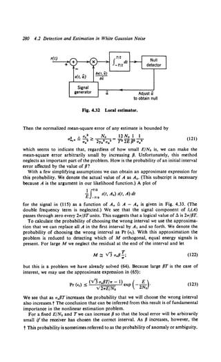
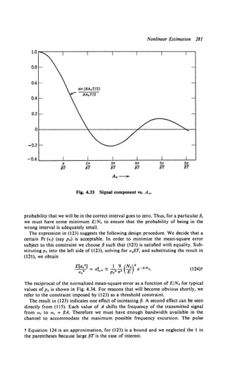
298. 282 4.2 Detection and Estimation in White Gaussian Noise
bandwidth is approximately 2w/Trad/sec. The maximum frequency shift is ± v3 f3aa.
Therefore the required channel bandwidth centered at we is approximately
.y- 2w l . ;-
2wWch ~ 2 3 f3aa + T = T(2v 3 f3aaT + 2w)
When aaf3T is large we can neglect the 2w and use the approximation
2wWch ~ 2VJ f3aa•
(l2Sa)
(l2Sb)
In many systems of interest we have only a certain bandwidth available. (This band-
width limitation may be a legal restriction or may be caused by the physical nature of
the channel.) If we assume that E/No is large enough to guarantee an acceptable
Pr (€1), then (125b) provides the constraint of the system design. We simply increase {3
until the available bandwidth is occupied. To find the mean-square error using this
design procedure we substitute the expression for f3aa in (l2Sb) into (121) and obtain
E[a2.] 2 18 No l
~ = aa,n = ,.• E (WchT)" (bandwidth constraint). (126)
We see that the two quantities that determine the mean-square error are E/N 0 , the
energy-to-noise ratio, and WchT, which is proportional to the time-bandwidth product
of the transmitted pulse. The reciprocal of the normalized mean-square error is
plotted in Fig. 4.34 for typical values of WchT.
The two families of constraint lines provide us with a complete design procedure
for a PFM system. For low values ofE/No the threshold constraint dominates. As E/No
increases, the MMSE moves along a fixed Po line until it reaches a point where the
available bandwidth is a constraint. Any further increase in E/No moves the MMSE
along a fixed {3 line.
The approach in which we consider two types of error separately is useful and
contributes to our understanding of the problem. To compare the results with other
systems it is frequently convenient to express them as a single number, the over-all
mean-square error.
We can write the mean-square error as
E(a.•) = a.T• = E[a,2 Jinterval error] Pr [interval error]
+ E[a.2 Jno interval error] Pr [no interval error] (127)
We obtained an approximation to Pr (€1) by collecting each incremental range of A
at a single value A,. With this approximation there is no signal component at the
other correlator outputs in Fig. 4.31. Thus, if an interval error is made, it is equally
likely to occur in any one of the wrong intervals. Therefore the resulting estimate d
will be uncorrelated with a.
E[a,2 Jinterval error] = E[(d - a)2 linterval error]
= E[d2 Jinterval error] + E[a2 linterval error]
- 2E[dalinterval error]. (128)
Our approximation makes the last term zero. The first two terms both equal aa2 •
Therefore
E[a."linterval error] = 2aa2• (129)
If we assume that p 0 is fixed, we then obtain by using (124) and (129) in (127)
a~Tn = E(a~•) = 2po + (1 -Po) _9_ (No)•e- EiNo. (130)
Ua ,.3p~ E

299. Nonlinear Estimation 283
101
"'
I
~
"' II
I
~
0
~
Threshold constraint
I I
E -
No
Fig. 4.34 Reciprocal of the mean-square error under threshold and bandwidth
constraints.
In this case the modulation index fJ must be changed as E/No is changed. For a fixed
fJ we use (121) and (123) to obtain
2 - 12 No [1 v3 a.{JT/rr -E/2N ] 2 v3 a.fJT/rr -E/2N
a - - - - - - e o + e o
•r• (a.{JT)2 2£ V2rrE/N0 V2rrE/No .
(131)
The result in (131) is plotted in Fig. 4.35, and we see that the mean-square error

300. 284 4.2 Detection and Estimation in White Gaussian Noise
exhibits a definite threshold. The reciprocal of the normalized mean-square error for
a PAM system is also shown in Fig. 4.35 (from 96). The magnitude of this improve-
ment can be obtained by dividing (121) by (96).
Thus the improvement obtained from PFM is proportional to the square of {1T. It is
important to re-emphasize that this result assumes E/No is such that the system is
above threshold. If the noise level should increase, the performance of the PFM
system can decrease drastically.
Our approach in this particular example is certainly plausible. We see,
however, that it relies on a two-step estimation procedure. In discrete
frequency modulation this procedure was a natural choice because it was
also a logical practical implementation. In the first example there was no
need for the two-step procedure. However, in order to obtain a parallel
set of results for Example 1 we can carry out an analogous two-step
analysis and similar results. Experimental studies of both types of systems
indicate that the analytic results correctly describe system performance.
It would still be desirable to have a more rigorous analysis.
We shall discuss briefly in the context of Example 2 an alternate
approach in which we bound the mean-square error directly. From (ll5)
we see that s(t, A) is an analytic function with respect to the parameter A.
Thus all derivatives will exist and can be expressed in a simple form:
{(2£)%
ans(t, A) = T ({3t)n( -l)<n-1)/2 cos (wet + {3At),
oAn (2E)Y2
T ({3t)n( -l)n12 sin (wet + {3At),
n odd,
(132)
n even.
This suggests that a generalization of the Bhattacharyya bound that we
developed in the problem section of Chapter 2 would enable us to get as
good an estimate of the error as desired. This extension is conceptually
straightforward (Van Trees [24]). For n = 2 the answer is still simple.
For n ;;::: 3, however, the required matrix inversion is tedious and it is
easier to proceed numerically. The detailed calculations have been carried
out [29]. In this particular case the series does not converge fast enough to
give a good approximation to the actual error in the high noise region.
One final comment is necessary. There are some cases of interest in
which the signal is not differentiable with respect to the parameter. A
simple example of this type of signal arises when we approximate the
transmitted signal in a radar system by an ideal rectangular pulse and
want to estimate the time of arrival of the returning pulse. When the noise
is weak, formulas for these cases can be developed easily (e.g., Mallinckrodt

301. t
E/No~
Fig. 4.35 Reciprocal of the total mean-square error.
285

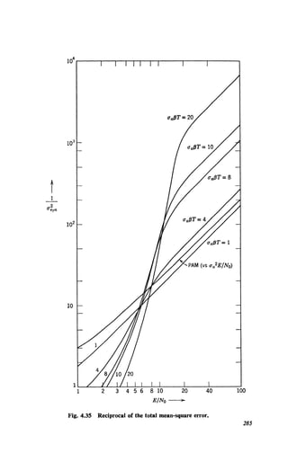
302. 286 4.2 Detection and Estimation in White Gaussian Noise
and Sollenberger [25], Kotelnikov [13], Manasse [26], Skolnik [27]).
For arbitrary noise levels we can use the approach in Example 2 or the
Barankin bound (e.g., Swerling [28]) which does not require differenti-
ability.
4.2.4 Summary: Known Signals in White Gaussian Noise
It is appropriate to summarize some of the important results that have
been derived for the problem of detection and estimation in the presence
of additive white Gaussian noise.
Detection. 1. For the simple binary case the optimum receiver can be
realized as a matched filter or a correlation receiver, as shown in Figs. 4.11
and 4.12, respectively.
2. For the general binary case the optimum receiver can be realized by
using a single matched filter or a pair of filters.
3. In both cases the performance is determined completely by the
normalized distance d between the signal points in the decision space,
d2 = ~o (E1 + Eo - 2pv'£;Fo). (133)
The resulting errors are
PF = erfc* e~7J + ~)• (134)
PM = err. end7J - g)· (135)
For equally-likely hypotheses and a minimum Pr (e) criterion, the total
error probability is
(136)
4. The performance of the optimum receiver is insensitive to small
signal variations.
5. For the M-ary case the optimum receiver requires at most M- 1
matched filters, although frequently M matched filters give a simpler
implementation. For M orthogonal signals a simple bound on the error
probability is
Pr (e) :s; M- 1 exp (-_§_)·
V27T(E/N0) 2No
(137)
6. A simple example of transmitting a sequence of digits illustrated the
idea of a channel capacity. At transmission rates below this capacity the

303. Model 287
Pr (4:) approaches zero as the length of encoded sequence approaches
infinity. Because of the bandwidth requirement, the orthogonal signal
technique is not efficient.
Estimation. 1. Linear estimation is a trivial modification of the detec-
tion problem. The optimum estimator is a simple correlator or matched
filter followed by a gain.
2. The nonlinear estimation problem introduced several new ideas. The
optimum receiver is sometimes difficult to realize exactly and an approxi-
mation is necessary. Above a certain energy-to-noise level we found that
we could make the estimation error appreciably smaller than in the linear
estimation case which used the same amount of energy. Specifically,
V [ ~ A] N0/2
ar a - ~ rT [os(t, A)]2
Jo oA dt.
(138)
As the noise level increased however, the receiver exhibited a threshold
phenomenon and the error variance increased rapidly. Above the threshold
we found that we had to consider the problem of a bandwidth constraint
when we designed the system.
We now want to extend our model to a more general case. The next
step in the direction of generality is to consider known signals in the
presence of nonwhite additive Gaussian noise.
4.3 DETECTION AND ESTIMATION IN NONWHITE GAUSSIAN NOISE
Several situations in which nonwhite Gaussian interference can occur
are of interest:
1. Between the actual noise source and the data-processing part of the
receiver are elements (such as an antenna and RF filters) which shape the
noise spectrum.
2. In addition to the desired signal at the receiver, there may be an
interfering signal that can be characterized as a Gaussian process. In
radar/sonar it is frequently an interfering target.
With this motivation we now formulate and solve the detection and
estimation problem. As we have seen in the preceding section, a close
coupling exists between detection and estimation. In fact, the development
through construction of the likelihood ratio (or function) is identical. We
derive the simple binary case in detail and then indicate how the results
extend to other cases of interest. The first step is to specify the model.

304. 288 4.3 Detection and Estimation in Nonwhite Gaussian Noise
When colored noise is present, we have to be more careful about our
model. We assume that the transmitted signal on hypothesis 1 is
0 5, t 5, T,
elsewhere.
(139)
Observe that s(t) is defined for all time. Before reception the signal is
corrupted by additive Gaussian noise n(t). The received waveform r(t)
is observed over the interval T.. 5, t 5, T1• Thus
r(t) = VE s(t) + n(t),
= n(t),
T1 5, t 5, T1 :H1
T1 5, t 5, T1 :H0•
(140)
Sometimes T1 will equal zero and T1 will equal T. In general, however,
we shall letT.. (:SO) and T1 (;::T) remain arbitrary. Specifically, we shall
frequently examine the problem in which 1j = -oo and T1 = +oo. A
logical question is; why should we observe the received waveform when
the signal component is zero? The reason is that the noise outside the
interval is correlated with the noise inside the interval, and presumably
the more knowledge available about the noise inside the interval the
better we can combat it and improve our system performance. A trivial
example can be used to illustrate this point.
Example. Let
v£s(t) = 1, O::>t::>1
(141)
= 0, elsewhere.
Let
n(t) = n, O::>t:52, (142)
where n is a Gaussian random variable. We can decide which hypothesis is true in the
following way:
I = J:r(t) dt - f r(t) dt. (143)
If
I= 0, say H 0
~ 0 say H,.
Clearly, we can make error-free decisions. Here we used the extended interval to
estimate the noise inside the interval where the signal was nonzero. Unfortunately,
the actual situation is not so simple, but the idea of using an extended observation
interval carries over to more realistic problems.
Initially, we shall find it useful to assume that the noise always contains
an independent white component. Thus
n(t) = w(t) + nc(t) (144)
where nc(t) is the colored noise component. Then,
Kn(t, u) = ~0 S(t - u) + Kc(t, u). (145)

305. Model 289
We assume the nc(t) has a finite mean-square value [E(nc2(t)) < oo for all
1j !5: t !5: T1] so Kc(t, u) is a square-integrable function over [Jj, T1].
The white noise assumption is included for two reasons:
1. The physical reason is that regardless of the region of the spectrum
used there will be a nonzero noise level. Extension of this level to infinity
is just a convenience.
2. The mathematical reason will appear logically in our development.
The white noise component enables us to guarantee that our operations
will be meaningful. There are other ways to accomplish this objective but
the white noise approach is the simplest.
Three logical approaches to the solution of the nonwhite noise problem
are the following:
1. We choose the coordinates for the orthonormal expansion of r(t) so
that the coefficients are statistically independent. This will make the con-
struction of the likelihood ratio straightforward. From our discussion in
Chapter 3 we know how to carry out this procedure.
2. We operate on r(t) to obtain a sufficient statistic and then use it to
perform the detection.
3. We perform preliminary processing on r(t) to transform the problem
into a white Gaussian noise problem and then use the white Gaussian
noise solution obtained in the preceding section. It is intuitively clear that
if the preliminary processing is reversible it can have no effect on the
performance of the system. Because we use the idea of reversibility
repeatedly, however, it is worthwhile to provide a simple proof.
Reversibility. It is easy to demonstrate the desired result in a general setting. In
Fig. 4.36a we show a system that operates on r(u) to give an output that is optimum
according to some desired criterion. (The problem of interest may be detection or
estimation.) In system 2, shown in Fig. 4.36b, we first operate on r(u) with a reversible
operation k[t, r(u)] to obtain z(t). We then design a system that will perform an
operation on z(t) to obtain an output that is optimum according to the same criterion
as in system 1. We now claim that the performances of the two systems are identical.
Clearly, system 2 cannot perform better than system 1 or this would contradict our
statement that system 1 is the optimum operation on r(u). We now show that system 2
cannot be worse than system 1. Suppose that system 2 were worse than system 1.
If this were true, we could design the system shown in Fig. 4.36c, which operates on
z(t) with the inverse of k[t, r(u)] to give r(u) and then passes it through system I.
This over-all system will work as well as system I (they are identical from the input-
output standpoint). Because the result in Fig. 4.36c is obtained by operating on z(t),
it cannot be better than system 2 or it will contradict the statement that the second
operation in system 2 is optimum. Thus system 2 cannot be worse than system I.
Therefore any reversible operation can be included to facilitate the solution. We
observe that linearity is not an issue, only the existence of an inverse. Reversibility
is only sufficient, not necessary. (This is obvious from our discussion of sufficient
statistics in Chapter 2.)

306. 290 4.3 Detection and Estimation in Nonwhite Gaussian Noise
I
r(u) Optimum I Output 1
----~operation :
1
Sysrm 1----~
Ti su $. Tr on r(u) 1
(a)
r(u) J I z(t)
-=--:---:-=-..;I k(t, r(u)j
1
1------+1
Ti$.u$.Tr
(b)
z(t)
(c)
Optimum operation on z(t)
Output 3
Output 2
Fig. 4.36 Reversibility proof: (a) system 1; (b) system 2; (c) system 3.
We now return to the problem of interest. The first two of these
approaches involve much less work and also extend in an easy fashion to
more general cases. The third approach however, using reversibility, seems
to have more intuitive appeal, so we shall do it first.
4.3.1 "Whitening" Approach
First we shall derive the structures of the optimum detector and
estimator. In this section we require a nonzero white noise level.
Structures. As a preliminary operation, we shall pass r(t) through a
linear time-varying filter whose impulse response is hw(t, u) (Fig. 4.37).
The impulse response is assumed to be zero for either t or u outside the
interval [T" T1]. For the moment, we shall not worry about realizability
r(t)
hw(t. u)
r,(t)
Fig. 4.37 " Whitening " filter.

307. "Whitening" Approach 291
and shall allow hw(t, u) to be nonzero for u > t. Later, in specific examples,
we also look for realizable whitening filters. The output is
IT/
r.(t) ~ hw(t, u) r(u) du
Tt
I~ I~
= hw(t, u)VE s(u) du + hw(t, u) n(u) du
Tt Tt
(146)
when H1 is true and
(147)
when H 0 is true. We want to choose hw(t, u) so that
Kn,(t, u) = E[n.(t) n.(u)] = S(t - u), T1 s t, u s T1• (148)
Observe that we have arbitrarily specified a unity spectral height for the
noise level at the output of the whitening filter. This is merely a convenient
normalization.
The following logical question arises:
What conditions on Kn(t, u) will guarantee that a reversible whitening
filter exists? Because the whitening filter is linear, we can show rever-
sibility by finding a filter hw- 1(t, u) such that
IT/
hw- 1(t, z) hw(z, u) dz = 8(t - u),
T,
T1 ::;; t, u ::;; T1• (149)
For the moment we shall assume that we can find a suitable set of
conditions and proceed with the development.
Because n.(t) is "white," we may use (22) and (23) directly (No = 2):
IT, IT'
ln A[r.(t)] = r.(u) s.(u) du - ! s!(u) du.
~ ~
(150)
We can also write this directly in terms of the original waveforms and
hw(t, u):
IT, IT' IT' -
ln A[r(t)] = du hw(u, z) r(z) dz hw(u, v)VE s(v) dv
T1 Tt Tt
IT, IT' IT'
- ! du hw(u, z)VEs(z) dz hw(u, v)VE s(v) dv.
Tt T, Tt (151)

308. 292 4.3 Detection und Estimation in Nonwhite Gaussian Noise
This expression can be formally simplified by defining a new function:
T1 < z, v < T1• (152)t
For the moment we can regard it as a function that we accidentally
stumbled on in an effort to simplify an equation. Later we shall see that it
plays a fundamental role in many of our discussions. Rewriting (151), we
have
JT
1 JT1
In A[r(t)] = r(z) dz Qn(z, v)VE s(v) dv
Tt T1
£JT1 JT1
- 2 s(z) dz Qn(z, v) s(v) dv.
T, T,
(153)
We can simplify (153) by writing
JTI
g(z) = Qn(z, v)VE s(v) dv,
T,
(154)
We have used a strict inequality in (154). Looking at (153), we see that g(z)
only appears inside an integral. Therefore, if g(z) does not contain singu-
larities at the endpoints, we can assign g(z) any finite value at the endpoint
and In A[r(t)] will be unchanged. Whenever there is a white noise com-
ponent, we can show that g(z) is square-integrable (and therefore contains
no singularities). For convenience we make g(z) continuous at the end-
points.
g(T1) = lim g(z),
z-+T1
-
g(T;) = lim g(z).
+
Z-+T
l
We see that the construction of the likelihood function involves a correla-
tion operation between the actual received waveform and a function g(z).
Thus, from the standpoint of constructing the receiver, the function g(z)
is the only one needed. Observe that the correlation of r(t) with g(t) is
simply the reduction of the observation space to a single sufficient statistic.
Three canonical receiver structures for simple binary detection are
t Throughout this section we must be careful about the endpoints of the interval.
The difficulty is with factors of 2 which arise because of the delta function in the noise
covariance. We avoid this by using an open interval and then show that endpoints
are not important in this problem. We suggest that the reader ignore the comments
regarding endpoints until he has read through Section 4.3.3. This strategy will make
these sections more readable.

309. " Whitening" Approach 293
-vE s(t)
(a)
r(t)
g(t)
(b)
-VE s(t)
(c)
Fig. 4.38 Alternate structures for colored noise problem.
shown in Fig. 4.38. We shall see that the first two are practical implementa-
tions, whereas the third affords an interesting interpretation. The modifica-
tion of Fig. 4.38b to obtain a matched filter realization is obvious. To
implement the receivers we must solve (149), (152), or (154). Rather than
finding closed-form solutions to these equations we shall content ourselves
in this section with series solutions in terms of the eigenfunctions and
eigenvalues of K0(t, u). These series solutions have two purposes:
1. They demonstrate that solutions exist.
2. They are useful in certain optimization problems.
After deriving these solutions, we shall look at the receiver performance
and extensions to general binary detection, M-ary detection, and estima-
tion problems. We shall then return to the issue of closed-form solutions.
The advantage of this approach is that it enables us to obtain an integrated
picture of the colored noise problem and many of its important features
without getting lost in the tedious details of solving integral equations.

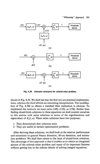
310. 294 4.3 Detection and Estimation in Nonwhite Gaussian Noise
Construction of Q,.(t, u) and g(t). The first step is to express Qn(t, u)
directly in terms of Kn(t, u). We recall our definition of hw(t, u). It is a
time-varying linear filter chosen so that when the input is n(t) the output
will be n.(t), a sample function from a white Gaussian process. Thus
lTI
n.(t) = hw(t, x) n(x) dx
Tl
1j5.t5.T
1 (155)
and
E[n.(t)n.(u)] = Kn.(t, u) = 8(t - u). 1j 5. t 5. T1• (156)
Substituting (155) into (156), we have
Tf
8(1 - u) = E JJhw(t, x) hw(u, z) n(x) n(z) dx dz. (157)
T,
By bringing the expectation inside the integrals, we have
Tf
8(t - u) = JJhw(t, x) hw(u, z) Kn(x, z) dx dz, T1 < t, u < T1• (158)
Tl
In order to get (158) into a form such that we can introduce Qn(t, u), we
multiply both sides by hw(t, v) and integrate with respect to t. This gives
iT/ iT1 iT1
hw(u, v) = dz hw(u, z) Kn(X, z) dx hw(t, v) hw(t, x) dt. (159)
T1 T1 T1
Looking at (152), we see that the last integral is just Qn(v, x). Therefore
(160)
This implies that the inner integral must be an impulse over the open
interval,
iTI
8(z - v) = Kn(X, z) Qn(V, x) dx,
T,
T1 < z, v < T1• (161)
This is the desired result that relates Qn(v, x) directly to the original
covariance function. Because Kn(x, z) is the kernel of many of the integral
equations of interest to us, Qn(v, x) is frequently called the inverse kernel.
From (145) we know that Kn(x, z) consists of an impulse and a well-
behaved term. A logical approach is to try and express Qn(v, x) in a
similar manner. We try a solution to (161) of the form
2
Qn(v, x) = No [S(v - x) - h0 (v, x)] Tl < v, X< T,. (162)

311. "Whitening" Approach 295
Substituting (145) and (162) into (161) and rearranging terms, we obtain
an equation that h0(v, x) must satisfy:
lVo IT'
T h0(V, z) + h0(v, x) Kc(X, z) dx = Kc(v, z),
T,
T1 < z, v < T1 (163)
This equation is familiar to us from the section on optimum linear filters
in Chapter 3 [Section 3.4.5; particularly, (3-144)]. The significance of this
similarity is seen by re-drawing the system in Fig. 4.38c as shown in Fig.
4.39. The function Qn(t, u) is divided into two parts. We see that the
output of the filter in the bottom path is precisely the minimum mean-
square error estimate of the colored noise component, assuming that H0
is true. If we knew n0 (t), it is clear that the optimum processing would
consist of subtracting it from r(t) and passing the result into a matched
filter or correlation receiver. The optimum receiver does exactly that,
except that it does not know n0(t); therefore it makes a MMSE estimate
iic(t) and uses it. This is an intuitively pleasing result of a type that we
shall encounter frequently.t
Assuming Ho is true,
r-·-------------------1
r(t) =llc(t) +w(t)
Unrealizable
1 filter
I Qn(t, u)
L--------------------~
Fig. 4.39 Realization of detector using an optimum linear filter.
t The reader may wonder why we care whether a result is intuitively pleasing, if we
know it is optimum. There are two reasons for this interest: (a) It is a crude error-
checking device. For the type of problems of interest to us, when we obtain a mathe-
matical result that is unintuitive it is usually necessary to go back over the model
formulation and the subsequent derivation and satisfy ourselves that either the model
omits some necessary feature of the problem or that our intuition is wrong. (b) In
many cases the solution for the optimum receiver may be mathematically intractable.
Having an intuitive interpretation for the solutions to the various Gaussian problems
equips us to obtain a good receiver by using intuitive reasoning when we cannot get a
mathematical solution.

312. 296 4.3 Detection and Estimation in Nonwhite Gaussian Noise
From our results in Chapter 3 (3.154) we can write a formal solution for
h0 (t, u) in terms of the eigenvalues of Kc(t, u). Using (3.154),
ao ){
h0 (t, u) = 2 )c + N, 12 cfot(t) cfot(u), T; < t, u < T1, (164)
I= 1 I 0
where •V and cfot(t) are the eigenvalues and eigenfunctions, respectively,
of K.(t, u). We can write the entire inverse kernel as
2 [ 00
)1c ]
Qn(t, u) = N, 8(t - u) - 2 ,c + N, 12 cfot(t) cfot(u) .
0 != 1 I 0
(165)
It is important to re-emphasize that our ability to write Qn(t, u) as an
impulse function and a well-behaved function rests heavily on our assump-
tion that there is a nonzero white noise level. This is the mathematical
reason for the assumption.
We can also write Qn(t, u) as a single series. We express the impulse in
terms of a series by using (3.128) and then combine the series to obtain
ao (No )-1 ao I
Qn(t, u) = 1~ 2 + ..{ cfot(t) cfot(u) = 1~ .? cp1(t) cp1(u), {166)
where
(167)
(T denotes total). The series in (166) does not converge. However, in most
cases Qn(t, u) is inside an integral and the overall expression will converge.
As a final result, we want to find an equation that will specify g(t)
directly in terms of Kn(t, z). We start with (154):
iTt
g(z) = Qn(z, v)VE s(v) dv,
T,
T1 < z < r,. (168)
The technique that we use is based on the inverse relation between Kn(t, z)
and Qn(t, z), expressed by (161). To get rid of Qn(z, v) we simply multiply
(168) by Kn(t, z), integrate with respect to z, and use (161). The result is
iTt
Kn(t, z) g(z) dz = VE s(t),
Tt
r, < t < r,. (169a)
Substituting (145) into (l69a), we obtain an equation for the open interval
(Tt. T1). Our continuity assumption after (154) extends the range to the
closed interval [Th T1]. The result is
N, iTt
2°g(t) + K.(t, z) g(z) dz = VE s(t),
Tt
T; ::::;; t ::::;; T1• (169b)
To implement the receiver, as shown in Fig. 4.38b, we would solve (l69b)

313. A Direct Derivation Using the Karhunen-Loeve Expansion 297
directly. We shall develop techniques for obtaining closed-form solutions
in 4.3.6. A series solution can be written easily by using (168) and (165):
( ) 2 . rr:. ( ) 2 ~ ,Vs1 (
g z = N, v E s z - N, L Ac N, 12 ¢>, z),
0 0 1=1 I + 0
(170)
where
IT!
s, = v£s(t) q,,(t) dt.
Tt
(171)
The first term is familiar from the white noise case. The second term
indicates the effect of nonwhite noise. Observe that g(t) is always a square-
integrable function over (T~o T1) when a white noise component is present.
We defer checking the endpoint behavior until4.3.3.
Summary
In this section we have derived the solution for the optimum receiver
for the simple binary detection problem of a known signal in nonwhite
Gaussian noise. Three realizations were the following:
1. Whitening realization (Fig. 4.38a).
2. Correlator realization (Fig. 4.38b).
3. Estimator-subtractor realization (Fig. 4.39).
Coupled with each of these realizations was an integral equation that
must be solved to build the receiver: 1. (158). 2. (169). 3. (163).
We demonstrated that series solutions could be obtained in terms of
eigenvalues and eigenfunctions, but we postponed the problem of actually
finding a closed-form solution. The concept of an "inverse kernel" was
introduced and a simple application shown. The following questions
remain:
1. How well does the system perform?
2. How do we find closed-form solutions to the integral equations of
interest?
3. What are the analogous results for the estimation problem?
Before answering these questions we digress briefly and rederive the
results without using the idea of whitening. In view of these alternate
derivations, we leave the proof that hw(t, u) is a reversible operator as an
exercise for the reader (Problem 4.3.1).
4.3.2 A Direct Derivation Using the Karhunen-Loeve Expansionj
In this section we consider a more fundamental approach. It is not only
t This approach to the problem is due to Grenander [30]. (See also: Kelly, Reed,
and Root [31].)

314. 298 4.3 Detection and Estimation in Nonwhite Gaussian Noise
more direct for this particular problem but extends easily to the general
case. The derivation is analogous to the one on pp. 250-253.
The reason that the solution to the white noise detection problem in
Section 4.2 was so straightforward was that regardless of the orthonormal
set we chose, the resulting observables r1o r2, ••• , rK were conditionally
independent.
From our work in Chapter 3 we know that we can achieve the same
simplicity if we choose an orthogonal set in a particular manner. Specifi-
cally, we want the orthogonal functions to be the eigenfunctions of the
integral equation (3-46)
(172)
Observe that the .{ are the eigenvalues of the colored noise process only.
(If Kc(t, u) is not positive-definite, we augment the set to make it complete.)
Then we expand r(t) in this coordinate system:
K K K
r(t) = l.i.m. L r1 cMt) = l.i.m. L s1 t/>1(t) + l.i.m. L n1 t/>1(t),
K-+oo i=l K-+oo i=l K-+ao i=l
Tt ~ t ~ T1, (173)
where
JTf (174)
r1 = r(t) t/>1(t) dt,
Tt
JTf
S; = VE s(t) tf>;(t) dt, (175)
Tt
and
f'
n1 = n(t) t/>1(t) dt. (176)
Tt
From {3.42) we know
E(n;) = 0, E(n1
n1) = .?8,Jo (177)
where
,T1::,. No , c
i-T+ I· (178)
Just as on p. 252 (20) we consider the first K coordinates. The likelihood
ratio is

315. A Direct Derivation with a Sufficient Statistic 299
Canceling common terms, letting K ~ oo, and taking the logarithm, we
obtain
(180)
Using (174) and (175), we have
In A[r(t)] = IT' dt JT' du r(t) 2: cMt) t1(u) VEs(u)
Tt Tt 1=1 ,1
- ~ JT' dt IT' du s(t) ~ cMt) t1(u) s(u). (181)
2 Tt Tt 1=1 ,!
From (166) we recognize the sum as Qn(t, u). Thus
IT, IT'
In A[r(t)] = dt du r(t) Qn(t, u)VE s(u)
Tt Tt
EfT' IT'
- 2 dt du s(t) Qn(t, u) s(u).
Tt Tt
(182)t
This expression is identical to (153).
Observe that if we had not gone through the whitening approach we
would have simply defined Qn(t, u) to fit our needs when we arrived at this
point in the derivation. When we consider more general detection problems
later in the text (specifically Chapter II.3), the direct derivation can easily
be extended.
4.3.3 A Direct Derivation with a Sufficient Statistict
For convenience we rewrite the detection problem of interest (140):
r(t) = VE s(t) + n(t),
= n(t),
T1 ~ t ~ T1:H1
T1 ~ t ~ T1 :Ho. (183)
In this section we will not require that the noise contain a white component.
From our work in Chapter 2 and Section 4.2 we know that if we can
write
r(t) = r 1 s(t) + y(t), (184)
t To proceed rigorously from (181) to (182) we require~~ 1 (s12/ll?2) < co (Grenander
[30]: Kelly, Reed, and Root [31]). This is always true when white noise is present.
Later, when we look at the effect of removing the white noise assumption, we shall
see that the divergence of this series leads to an unstable test.
t This particular approach to the colored noise problem seems to have been developed
independently by several people (Kailath [32]; Yudkin [39]). Although the two
derivations are essentially the same, we follow the second.

316. 300 4.3 Detection and Estimation in Nonwhite Gaussian Noise
where r1 is a random variable obtained by operating on r(t) and demon-
strate that:
(a) r1 and y(t) are statistically independent on both hypotheses,
(b) the statistics of y(t) do not depend on which hypothesis is true,
then r1 is a sufficient statistic. We can then base our decision solely on r1
and disregard y(t). [Note that conditions (a) and (b) are sufficient, but not
necessary, for r1 to be a sufficient statistic (see pp. 35-36).]
To do this we hypothesize that r1 can be obtained by the operation
IT!
r1 = r(u) g(u) du
T,
(185)
and try to find a g(u) that will lead to the desired properties. Using (185),
we can rewrite {184) as
r(t) = (s1 + n1) s(t) + y(t) :H1
= n1 s(t) + y(t) :H0 • (186)
where
(187)
and
IT!
n1 t:=. n(u) g(u) du.
T,
(188)
Because a sufficient statistic can be multiplied by any nonzero constant
and remain a sufficient statistic we can introduce a constraint,
lTI
s(u)g(u) du = 1.
Tt
(189a)
Using (189a) in (187), we have
s1 = VE. (189b)
Clearly, n1 is a zero-mean random variable and
n(t) = n1 s(t) + y(t), (190)
This puts the problem in a convenient form and it remains only to find
a condition on g(u) such that
E[n1y(t)] = 0, T, ~ t ~ T1, (191)
or, equivalently,
E{n1 [n(t) - n1 s(t)]} = 0, T1 ~t~Tt> (192)
or
E[n1 ·n(t)] = E[n12] s(t), T1 ~ t ~ Tt. (193)

317. Detection Performance 301
Using (188)
Tf
I:.' Kn(t, u) g(u) du = s(t) JJg(a) Kn(a, fJ) g(fJ) da dfJ,
Tt
(194)
Equations 189a and 194 will both be satisfied if
IT/
Kn(t, u) g(u) du = vEs(t),
T,
(195)
[Substitute (195) into the right side of (194) and use (189a).] Our sufficient
statistic r1 is obtained by correlating r(u) with g(u). After obtaining r1 we
use it to construct a likelihood ratio test in order to decide which hypothesis
is true.
We observe that (195) is over the closed interval [1!, T1], whereas (169a)
was over the open interval (T;, T1). The reason for this difference is that
in the absence of white noise g(u) may contain singularities at the end-
points. These singularities change the likelihood ratio so we can no longer
arbitrarily choose the endpoint values. An advantage of our last derivation
is that the correct endpoint conditions are included. We should also
observe that if there is a white noise component {195) and (169a) will give
different values for g(1j) and g(T1). However, because both sets of values
are finite they lead to the same likelihood ratio.
In the last two sections we have developed two alternate derivations of
the optimum receiver. Other derivations are available (a mathematically
inclined reader might read Parzen [40], Hajek [41], Galtieri [43], or
Kadota [45]). We now return to the questions posed on p. 297.
4.3.4 Detection Performance
The next question is: "How does the presence of colored noise affect
performance?" In the course ofanswering it a number ofinteresting issues
appear. We consider the simple binary detection case first.
Performance: Simple Binary Detection Problem. Looking at the receiver
structure in Fig. 4.38a, we see that the performance is identical to that of
a receiver in which the input signal is s*(t) and the noise is white with a
spectral height of 2. Using (10) and (11), we have
(196)

318. 302 4.3 Detection and Estimation in Nonwhite Gaussian Noise
Thus the performance index d2 is simply equal to the energy in the
whitened signal. We can also express d2 in terms of the original signal.
d2 = J2 dt[J2 hw(t,u)VEs(u)du][J;' hw(t,z)VEs(z)dz]· (197)
We use the definition of Q,.(u, z) to perform the integration with respect
to t. This gives
TJ
(198)
d2 = E JJdu dz s(u) Q,.(u, z) s(z)
Tt
J
TJ
d2 = VE du s(u) g(u).
Tt
It is clear that the performance is no longer independent of the signal
shape. The next logical step is to find the best possible signal shape. There
are three cases of interest:
1. T1 = 0, T1 = T: the signal interval and observation interval coincide.
2. T1 < 0, T1 > T: the observation interval extends beyond the signal
interval in one or both directions but is still finite.
3. T1 = -oo, T1 = oo: the observation interval is doubly infinite.
We consider only the first case.
Optimum Signal Design: Coincident Intervals. The problem is to con-
strain the signal energy E and determine how the detailed shape of s(t)
affects performance. The answer follows directly. Write
00 c'~ rl
Q,.(t, u) = 1~ 2°+ >./ cPt(t) t/>t(u). (199)
Then
00 2
d2 = 2: s, • (200)
!=1 No/2 + Ate
where
s1 = LT VE s(t) cPt(t) dt. (201)
Observe that
00
2 s,2 = E, (202)
I= 1
because the functions are normalized.
Looking at (200), we see that d2 is just a weighted sum of the s12•
Because (202) constrains the sum of the s12, we want to distribute the
energy so that those s1 with large weighting are large. If there exists a

319. Detection Performance 303
smallest eigenvalue, say ></ = >.~10, then d2 will be maximized by letting
s1 = VE and all other s1 = 0. There are two cases of interest:
1. If Kc(t, u) is positive-definite, the number of eigenvalues is infinite.
There is no smallest eigenvalue. We let si = v'E and all other s1 = 0.
Then, assuming the eigenvalues are ordered according to decreasing size,
d2~2E
No
as we increase j. For many of the colored noises that we encounter in
practice (e.g., the one-pole spectrum shown in Fig. 3.9), the frequency of
the eigenfunction increases as the eigenvalues decrease. In other words, we
increase the frequency of the signal until the colored noise becomes
negligible. In these cases we obtain a more realistic signal design problem
by including a bandwidth constraint.
2. If Kc(t, u) is only nonnegative definite, there will be zero eigenvalues.
If s(t) is the eigenfunction corresponding to any one of these eigenvalues,
then
d2 = 2E.
No
We see that the performance of the best signal is limited by the white
nmse.
Singularity. It is easy to see the effect of removing the white noise by
setting N0 equal to zero in (200). When the colored noise is positive-
definite (Case 1), all eigenvalues are nonzero. We can achieve perfect
detection (d2 = oo) if and only if the sum
(203)
diverges.
It can be accomplished by choosing s(t) so that s12 is proportional to>./.
We recall that
L V = 1
Kc(t, t) dt < M.
oo fT
1=1 T,
The right side is finite by our assumption below (145). Thus the energy in
the signal (E = ,21
";. 1 s12) will be finite. If there were a white noise com-
ponent, we could not achieve this proportionality for all i with a finite
energy signal. In (Case 2) there are zero eigenvalues. Thus we achieve
d2 = oo by choosing s(t) = (Mt) for any i that has a zero eigenvalue.
These two cases are referred to as singular detection. For arbitrarily
small time intervals and arbitrarily small energy levels we achieve perfect

320. 304 4.3 Detection and Estimation in Nonwhite Gaussian Noise
detection. We know that this kind of performance cannot be obtained in
an actual physical situation. Because the purpose of our mathematical
model is to predict performance of an actual system, it is important that
we make it realistic enough to eliminate singular detection. We have
eliminated the possibility of singular detection by insisting on a nonzero
white noise component. This accounts for the thermal noise in the receiver.
Often it will appear to be insignificant. If, however, we design the signal
to eliminate the effect of all other noises, it becomes the quantity that
limits the performance and keeps our mathematical model from predicting
results that would not occur in practice.
From (196) we know that d2 is the energy in the whitened signal.
Therefore, if the whitened signal has finite energy, the test is not singular.
When the observation interval is infinite and the noise process is stationary
with a rational spectrum, it is easy to check the finiteness of the energy of
s*(t). We first find the transfer function of the whitening filter. Recall that
(204)
We require that n.(t) be white with unity spectral height. This implies that
co
If du dz hw(u) hw(z) Kn(t - u + z - v) = S(t - v),
-00 < t, v < 00. (205)
Transforming, we obtain
(206a)
or
(206b)
Now assume that Sn(w) has a rational spectrum
(207a)
We define the difference between the order of denominator and numerator
(as a function of w2) as r.
r ~ p- q (207b)
If n(t) has finite power then r ~ I. However, if the noise consists of
white noise plus colored noise with finite power, then r = 0. Using (207a)

321. Singularity 305
in (206b), we see that we can write HwUw) as a ratio of two polynomials
injw.
(208a)
In Chapter 6 we develop an algorithm for finding the coefficients. For the
moment their actual values are unimportant. Dividing the numerator by
the denominator, we obtain
H U
. ) - f, U )' f, u· )'-1 ~" R(jw) (208b)
w w- r w + r-1 w +···+;o + bq{jw)q +···+ bo'
where fn ... , fo are constants and R(jw) is the remainder polynomial of
order less than q. Recall that (jw)' in the frequency domain corresponds to
taking the rth derivative in the time domain. Therefore, in order for the
test to be nonsingular, the rth derivative must have finite energy. In other
words, if
J
oo (d's(t))2
-d, dt < M
-oo t
(209)
the test is nonsingular; for example, if
S (w) = 2aan2
n w2 + a2
(210a)
then
p-q=r=I (210b)
and s'(t) must have finite energy. If we had modeled the signal as an ideal
rectangular pulse, then our model would indicate perfect detectability.
We know that this perfect detectability will not occur in practice, so we
must modify our model to accurately predict system performance. In this
case we can eliminate the singular result by giving the pulse a finite rise
time or by adding a white component to the noise. Clearly, whenever there
is finite-power colored noise plus an independent white noise component,
the integral in (209) is just the energy in the signal and singularity is never
an Issue.
Our discussion has assumed an infinite observation interval. Clearly, if
the test is nonsingular on the infinite interval, it is nonsingular on the finite
interval because the performance is related monotonically to the length of
the observation interval. The converse is not true. Singularity on the
infinite interval does not imply singularity on the finite interval. In this
case we must check (203) or look at the finite-time whitening operation.
Throughout most of our work we retain the white noise assumption so
singular tests never arise. Whenever the assumption is removed, it is
necessary to check the model to ensure that it does not correspond to a
singular test.

322. 306 4.3 Detection and Estimation in Nonwhite Gaussian Noise
General Binary Receivers. Our discussion up to this point has considered
only the simple binary detection problem. The extension to general binary
receivers is straightforward. Let
r(t) = VB;_ s1(t) + n(t),
r(t) = v'E0 s0(t) + n(t),
(211)
where s0(t) and s1(t) are normalized over the interval (0, T) and are zero
elsewhere. Proceeding in exactly the same manner as in the simple binary
case, we obtain the following results. One receiver configuration is shown
in Fig. 4.40a. The function gl!.(t) satisfies
sit) ~ v'£1 s1(t) - v'Eo so(I)
(212)
The performance is characterized by d2 :
Tt
d2 = JJs.1(t) Qn(t, u) sl!.(u) dt du. (213)
Tt
The functions Kn(t, u) and Qn(t, u) were defined in (145) and (161),
respectively. Ali an alternative, we can use the whitening realization shown
in Fig. 4.40b. Here hw(t, u) satisfies (158) and
iTt
sl!..(t) ~ hw(t, u) siu) du,
T,
(214)
r(t) H1 or Ho
TiS t S'If
H1 or Ho
(b)
Fig. 4.40 (a) Receiver configurations: general binary problem, colored noise;
(b) alternate receiver realization.

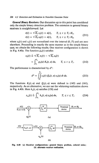
323. Estimation 307
The performance is characterized by the energy in the whitened difference
signal:
(215)
The M-ary detection case is also a straightforward extension (see
Problem 4.3.5). From our discussion of white noise we would expect that
the estimation case would also follow easily. We discuss it briefly in the
next section.
4.3.5 Estimation
The model for the received waveform in the parameter estimation
problem is
r(t) = s(t, A) + n(t), (216)
The basic operation on the received waveform consists of constructing the
likelihood function, for which it is straightforward to derive an expression.
If, however, we look at (98-lOI), and (146-153), it is clear that the answer
will be:
iT! iT1
In A1 [r(t), A] = r(z) dz Q,.(z, v) s(v, A) dv
T1 T1
iT! iT!
- t dz s(z, A) Q,.(z, v) s(v, A) dv. (217)
T1 T1
This result is analogous to (153) in the detection problem. If we define
iT!
g(z, A) = Q,.(z, v) s(v, A) dv,
T,
T1 < z < T1, (218)
or, equivalently,
iT!
s(v, A) = K,.(v, z) g(z, A) dz,
Ti
T1 < v < r,, (219)
(217) reduces to
iT!
In A1 [r(t), A] = r(z) g(z, A) dz
T,
iT!
- ! s(z, A) g(z, A) dz.
T,
(220)
The discussions in Sections 4.2.2 and 4.2.3 carry over to the colored noise
case in an obvious manner. We summarize some of the important results
for the linear and nonlinear estimation problems.

324. 308 4.3 Detection and Estimation in Nonwhite Gaussian Noise
Linear Estimation. The received waveform is
r(t) = AVEs(t) + n(t), (221)
where s(t) is normalized [0, T] and zero elsewhere. Substituting into (218),
we see that
g(t, A) = A g(t), (222)
where g(t) is the function obtained in the simple binary detection case by
solving (169).
Thus the linear estimation problem is essentially equivalent to simple
binary detection. The estimator structure is shown in Fig. 4.41, and the
estimator is completely specified by finding g(t). If A is a nonrandom
variable, the normalized error variance is
(223)
where d2 is given by (198). If A is a value of a random variable a with a
Gaussian a priori density, N(O, aa), the minimum mean-square error is
(224)
(These results correspond to (96) and (97) in the white noise case) All
discussion regarding singular tests and optimum signals carries over
directly.
Nonlinear Estimation. In nonlinear estimation, in the presence ofcolored
noise, we encounter all the difficulties that occur in the white noise case.
In addition, we must find either Qn(t, u) or g(t, A). Because all of the
results are obvious modifications of those in 4.2.3, we simply summarize
the results :
l. A necessary, but not sufficient, condition on am1:
J
r, Jr' os(u A)l
0 = dt du [r(t) - s(t, A)] Qn(t, u) oA - .
T1 T1 A=am1
r(t)
g(t)
>--- am! or amap
(depending on
choice of gain)
Fig. 4.41 Linear estimation, colored noise.
(225)

325. Solution Techniques for Integral Equations 309
2. A necessary, but not sufficient, condition on dma.p (assuming that a
has a Gaussian a priori density):
tlma.p = Cla2 IT' dt [r(t) - s(t, A)] IT' du Qn(t, u) os~AA)l . (226}
Tt T, A=<lmap
3. A lower bound on the variance of any unbiased estimate of the non-
random variable A:
or, equivalently,
Var (a - A) ~ [ {T' os(t, A) og(t, A) dt] -1.
JT, oA oA
(227b)
4. A lower bound on the mean-square error in the estimate of a zero-
mean Gaussian random variable a:
5. A lower bound on the variance of any unbiased estimate of a non-
random variable for the special case of an infinite observation interval and
a stationary noise process:
V ( A - A) [J 00
oS*Uw, A) s -1( ) oSUw, A) dw] -1
ar a ~ - oo oA n w oA 21T , (229)
where
SUw, A) Q J_'"oo s(t, A)e-1wt dt.
As we discussed in 4.2.3, results of this type are always valid, but we must
always look at the over-all likelihood function to investigate their useful-
ness. In other words, we must not ignore the threshold problem.
The only remaining issue in the matter of colored noise is a closed form
solution for Qn(t, u) or g(t). We consider this problem in the next section.
4.3.6 Solution Techniques for Integral Equations
As we have seen above, to specify the receiver structure completely we
must solve the integral equation for g(t) or Qn(t, u).

326. 310 4.3 Detection and Estimation in Nonwhite Gaussian Noise
In this section we consider three cases of interest:
1. Infinite observation interval; stationary noise process.
2. Finite observation interval; separable kernel.
3. Finite observation interval; stationary noise process.
Infinite Observation Interval; Stationary Noise. In this particular case
T1 = -oo, T1 = oo, and the covariance function of the noise is a function
only of the difference in the arguments. Then (161) becomes
8(z - v) = J:"" Qn(X - z) Kn(V -x) dx, -00 < v, z < 00, (230)
where we assume that we can find a Qn(x, z) of this form. By denoting
the Fourier transform of Kn(r) by Sn(w) and the Fourier transform of
Qn(r) by SQ(w) and transforming both sides of (230) with respect to
T = z - v, we obtain
(231)
We see that SQ(w) is just the inverse of the noise spectrum. Further, in the
stationary case (152) can be written as
Qn(z - v) = J:"" hw(u - z) hw(u - v) du. (232)
By denoting the Fourier transform of hw(r) by Hw(jw), we find that (232)
implies
(233)
Finally, for the detection and linear estimation cases (154) is useful.
Transforming, we have
(234)
where the subscript oo indicates that we are dealing with an infinite interval.
To illustrate the various results, we consider some particular examples.
Example 1. We assume that the colored noise component has a rational spectrum.
A typical case is
(235)
and
(236)

327. Then
Solution Techniques for Integral Equations 311
w2 + k2
SQ(w) = •
No (w2 + k2(1 + A)]
2
(237)
where A = 4un"fkNo. Writing
SQ(w) = (jw + k)(-jw + k) ,
(N0 /2)(jw + kv' 1 + A)(-jw + kv' 1 + A)
(238)
we want to choose an Hw(jw) so that (233) will be satisfied. To obtain a realizable
whitening filter we assign the term (jw + k(1 + A)Yz) to Hw(jw) and its conjugate to
H!Uw). The term (jw + k) in the numerator can be assigned to Hw(jw) or H!(jw}.
Thus there are two equally good choicest for the whitening filter:
. (2)Yz jw + k (2)Yz[ k(v'f+A- 1)]
Hw1 (jw) = No jw + k(l + A)Yz = No 1 - jw + kVl +A (239)
and
. ( 2 )Yo -jw + k ( 2 )Yo[ k(v'f""+'"A. + 1)]
Hw.(Jw) = No jw + k(1 + A)Yz = No -1 + jw + kV1 +A . (240)
Thus the optimum receiver (detector) can be realized in the whitening forms shown
in Fig. 4.42. A sketch of the waveforms for the case in which s(t) is a rectangular pulse
is also shown. Three observations follow:
1. The whitening filter has an infinite memory. Thus it uses the entire past of r(t)
to generate the input to the correlator.
2. The signal input to the multiplier will start at t = 0, but even after time t = T
the input will continue.
3. The actual integration limits are (0, oo), because one multiplier input is zero
before t = 0.
It is easy to verify that these observations are true whenever the noise consists of
white noise plus an independent colored noise with a rational spectrum. It is also
true, but less easy to verify directly, when the colored noise has a nonrational
spectrum. Thus we conclude that under the above conditions an increase in observa-
tion interval will always improve the performance. It is worthwhile to observe that if
we use Hw1(jw) as the whitening filter the output of the filter in the bottom path will
be iic,(t), the minimum mean-square error realizable point estimate of nc(t). We shall
verify that this result is always true when we study realizable estimators in Chapter 6.
Observe that we can just as easily (conceptually, at least) operate with SQ(w)
directly. In this particular case it is not practical, but it does lead to an interesting
interpretation of the optimum receiver. Notice that SQ(w) corresponds to an un-
realizable filter. We see that we could pass r(t) through this filter and then cross-
correlate it with s(t), as shown in Figure 4.43a. Observe that the integration is just
over [0, T] because s(t) is zero elsewhere; '**(t), 0 s t s T, however, is affected by
r(t), -oo < t < oo. We see that the receiver structure in Fig. 4.43b is the estimator-
subtractor configuration shown in Fig. 4.39. Therefore the signal at the output of the
bottom path must be iic.(t), the minimum mean-square error unrealizable estimate of
t There are actually an infinite number, for we can cascade Hw1(jw) with any filter
whose transfer function has unity magnitude. Observe that we choose a realizable
filter so that we can build it. Nothing in our mathematical model requires realizability.

328. 312 4.3 Detection and Estimation in Nonwhite Gaussian Noise
r(t)
(a)
r(t)
(b)
Fig. 4.42 "Optimum receiver": "whitening" realizations: (a) configuration 1;
(b) configuration 2.
nc(t). This can be verified directly by substituting (235) and (236) into (3.239). We
shall see that exactly the same result occurs in the general colored noise detection
problem. Comparing Figs. 4.42 and 4.43, we see that they both contain estimates of
colored noise but use them differently.
As a second example we investigate what happens when we remove the
white noise component.
Example 2.
(241)
Then
w2 + k2
Sg(w) = 2kan2 . (242)
If we use a whitening realization, then one choice for the whitening filter is
Hw(jw) = _1 l Uw + k). (243)
V 2kan2

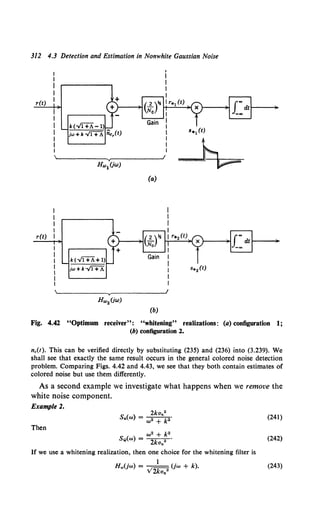
329. Solution Techniques for Integral Equations 313
r(t)
s(t)
(a)
r(t)
(b)
Fig. 4.43 Optimum receiver: estimator-subtractor interpretation.
Thus the whitening filter is a ditferentiator and gain in parallel (Fig. 4.44a).
Alternately, using (234), we see that G"'(jw) is,
. v£ S(jw) v£ 2 2 •
G«~(Jw) = S.(w) = 2ka.• (w + k ) S(Jw). (244)
Remembering that jw in the frequency domain corresponds to differentiation in the
time domain, we obtain
r(t)
v£
g"'(t) = 2ka.• [-s"(t) + k2 s(t)],
_ ~ (s'(t) + ks(t)]
-y2ku.2
(a)
-yE [-sN(t) +k2 s(t)]
2ku 2
n (b)
Fig. 4.44 Optimum receiver: no white noise component.
(245)

330. 314 4.3 Detection and Estimation in Nonwhite Gaussian Noise
as shown in Fig. 4.44b. Observe that s(t) must be differentiable everywhere in the
interval - oo < t < oo; but we assume that s(t) = 0, t < 0, and t > T. Therefore
s(O) and s(T) must also be zero. This restriction is intuitively logical. Recall the loose
argument we made previously: if there were a step in the signal and it was differen-
tiated formally, the result would be an impulse plus a white noise and lead to perfect
detection. This is obviously not the actual physical case. By giving the pulse a finite
rise time or including some white noise we avoid this condition.
We see that the receiver does not use any of the received waveform outside the
interval 0 :5 t :5 T, even though it is available. Thus we should expect the solution
for T. = 0 and T1 = T to be identical. We shall see shortly that it is.
Clearly, this result will hold whenever the noise spectrum has only poles, because
the whitening filter is a weighted sum of derivative operators. When the total noise
spectrum has zeros, a longer observation time will help the detectability. Observe that
when independent white noise is present the total noise spectrum will always have
zeros.
Before leaving the section, it is worthwhile to summarize some of the
important results.
1. For rational colored noise spectra and nonzero independent white
noise, the infinite interval performance is better than any finite observation
interval. Thus, the infinite interval performance which is characterized by
doo2 provides a simple bound on the finite interval performance. For the
particular one-pole spectrum in Example 1 a realizable, stable whitening
filter can be found. This filter is not unique. In Chapter 6 we shall again
encounter whitening filters for rational spectra. At that time we demons-
trate how to find whitening filters for arbitrary rational spectra.
2. For rational colored noise spectra with no zeros and no white noise
the interval in which the signal is nonzero is the only region of importance.
In this case the whitening filter is realizable but not stable (it contains
differentiators).
We now consider stationary noise processes and a finite observation
interval.
Finite Observation Interval; Rational Spectrat. In this section we consider
some of the properties of integral equations over a finite interval. Most of
the properties have been proved in standard texts on integral equations
(e.g., [33] and [34]). They have also been discussed in a clear manner in
the detection theory context by Helstrom [14]. We now state some simple
properties that are useful and work some typical examples.
The first equation of interest is (195),
IT!
VE s(t) = g(u) Kn(t, u) du;
Ti
(246)
t The integral equations in Section 3.4 are special cases of the equations studied in
this section. Conversely, if the equation specifying the eigenfunctions and eigenvalues
has already been solved, then the solutions to the equations in the section follow
easily.

331. Solution Techniques for Integral Equations 315
where s(t) and Kn(t. u) are known. We want to solve for g(t). Two special
cases should be considered separately.
Case 1. The kernel Kn(t, u) does not contain singularities. Physically, this
means that there is no white noise present. Here (246) is a Fredholm
equation of the first kind, and we can show (see [33]) that if the range
(Tj, T1) is finite a continuous square-integrable solution will not exist in
general. We shall find that we can always obtain a solution if we allow
singularity functions (impulses and their derivatives) in g(u) at the end
points of the observation interval.
In Section 4.3.7 we show that whenever g(t) is not square-integrable
the test is unstable with respect to small perturbations in the model
assumptions.
We have purposely excluded Case No. l from most of our discussion on
physical grounds. In this section we shall do a simple exercise to show the
result of letting the white noise level go to zero. We shall find that in the
absence of white noise we must put additional restrictions on s(t) to get
physically meaningful results.
Case 2. The noise contains a nonzero white-noise term. We may then write
Kn(t, u) = ~0 8(t - u) + Kc(t, u),
where Kc(t, u) is a continuous square-integrable function. Then
is the equation of interest,
N, fTI
v'E s(t) = 2°g(t) + Kc(t, u) g(u) du,
T,
(247)
(169b)
(248)
This equation is called a Fredholm equation of the second kind. A con-
tinuous, square-integrable solution for g(t) will always exist when Kc(t, u)
is a continuous square-integrable function.
We now discuss two types of kernels in which straightforward procedures
for solving (246) and (248) are available.
Type A (Rational Kernels). The noise nc(t) is the steady-state response of a
lumped, linear passive network excited with white Gaussian noise. Here
the covariance function depends only on (t - u) and we may write
(249)
The transform is
S ( ) J"' K ( ) - iw• d fl N(w2)
c w = -"' c T e T - D(w2) (250)

332. 316 4.3 Detection and Estimation in Nonwhite Gaussian Noise
and is a ratio of two polynomials in w2• The numerator is of order q in w2
and the denominator is of order p in w2• We assume that nc(t) has finite
power so p - q ~ 1. Kernels whose transforms satisfy (250) are called
rational kernels.
Integral equations with this type of kernel have been studied in detail
in [35-37], [47, pp. 1082-1102] [54, pp. 309-329], and [62). We shall
discuss a simple example that illustrates the techniques and problems
involved.
Type B (Separable Kernels). The covariance function of the noise can be
written as
K
Kc(t, u) = L .;4>t(t) 4>t(u), (251)
I= 1
where K is.finite. This type ofkernel is frequently present in radar problems
when there are multiple targets. As we shall see in a later section, the
solution to (246) is straightforward. We refer to this type of kernel as
separable. Observe that if we had allowed K = oo all kernels would be
considered separable, for we can always write
co
Kc(t, u) = L .1 4>1(1) 4>t(u), (252)
I= 1
where the .1 and 4>1(t) are the eigenvalues and eigenfunctions. Clearly, this
is not a practical solution technique because we have to solve another
integral equation to find the 4>1(t).
We consider rational kernels in this section and separable kernels in the
next.
Fredholm Equations ofthe First Kind: Rational Kernels. The basic technique
is to find a differential equation corresponding to the integral equation.
Because of the form of the kernel, this will be a differential equation with
constant coefficients whose solution can be readily obtained. In fact, the
particular solution of the differential equation is precisely the goo(t) that
we derived in the last section (234). An integral equation with a rational
kernel corresponds to a differential equation plus a set of boundary con-
ditions. To incorporate the boundary conditions, we substitute the par-
ticular solution plus a weighted sum of the homogeneous solutions back
into the integral equation and try to adjust the weightings so that the
equation will be satisfied. It is at this point that we may have difficulty.
To illustrate the technique and the possible difficulties we may meet, we

333. Fredholm Equations ofthe First Kind 317
consider a simple example. The first step is to show how g co(t) enters the
picture. Assume that
(253)
and recall that
S(t - u) = Ico eJro<t-u) dw.
-oo 2'17
(254)
Differentiation with respect to t gives
p S(t - u) = jw elro<t-u> _,
I"' dw
-co 2'17
(255)
where p ~ dfdt. More generally,
N( -p2) S(t- u) =I"' N(w2)e1ru<t-u> dw.
-oo 2'17
(256)
In an analogous fashion
D( -p2) Kn(t - u) = I"' D(w2) Sn(w) eJru<t-u) dw_ (257)
-co 2'17
From (253) we see that the right sides of (256) and (257) are identical.
Therefore the kernel satisfies the differential equation obtained by equating
the left sides of (256) and (257):
Now the integral equation of interest is
VE s(t) = JT' Kn(t - u) g(u) du,
r,
Operating on both sides of this equation with D(-p2), we obtain
Using (258) on the right-hand side, we have
D(-p2)VE s(t) = N( -p2) g(t),
(258)
(259)
(261)
but from our previous results (234) we know that if the observation
interval were infinite,
(262)
or
-00 < t < 00. (263)

334. 318 4.3 Detection and Estimation in Nonwhite Gaussian Noise
Thus g""(t) corresponds to the particular solution of (261). There are also
homogeneous solutions to (261):
0 = N( -p2) gh,(t), i = 1, 2, ... , 2q. (264)
We now add the particular solution g""(t) to a weighted sum of the 2q
homogeneous solutions gh1
(t), substitute the result back into the integral
equation, and adjust the weightings to satisfy the equation. At this point
the discussion will be clearer if we consider a specific example.
Example. We consider (246) and use limits [0, T] for algebraic simplicity.
or
Thus
and
The differential equation (261) is
VE( -s"(t) + k 2s(t)) = 2kan2 g(t).
The particular solution is
v£
g.,(t) = 2kan2 [-s"(t) + k2s(t)]
and there is no homogeneous solution as
q = 0.
Substituting back into the integral equation, we obtain
VE s(t) = an2 J:exp (-kit - ui) g(u) du,
For g(t) to be a solution, we require,
Os;ts;T,
(t) - ·{ -kt r· +ku[-s"(u) + k•s(u)] d
s - an e Joe 2kan• u
+ e+kt rT e-ku[-s"(U) +2k2S(U)] du}•
J, 2kan
Os;ts;T.
(265)
(266)
(267)
(268)
(269)
(270)
(271)
(272)
(273)
Because there are no homogeneous solutions, there are no weightings to adjust.
Integrating by parts we obtain the equivalent requirement,
0 = e-kt{~ [s'(O) - ks(O)l}
- e+k<t-n{;k [s'(T) + ks(T)l} (274)
Clearly, the two terms in brackets must vanish independently in order for g .,(t) to
satisfy the integral equation. //they do, then our solution is complete. Unfortunately,
the signal behavior at the end points often will cause the terms in the brackets to be

335. Fredholm Equations of the First Kind 319
nonzero. We must add something to g.,(t) to cancel the e-kt and ek<t-T> terms. We
denote this additional term by g 6(t) and choose it so that
an2 f exp (-kit- u)g.(u) du
I 1
= - 2k [s'(O) - ks(O)] e-kt + 2k [s'(T) + ks(T)] e+k<t-Tl, 0 s t s T. (275)
To generate an e-kt term g.(u) must contain an impulse c1 ll(u). To generate an
e+k<t-T> term g6(u) must contain an impulse c. ll(u - T). Thus
(276)
where
k s(O) - s'(O)
cl = ka." '
k s(T) + s'(T)
c2 = ka.2 '
(277)
to satisfy (274).t Thus the complete solution to the integral equation is
g(t) = g.,(t) + g.(t), 0 s t S T. (278)
From (!53) and (154) we see that the output of the processor is
I= fr(t)g(t)dt
= ~r(O) + ~r(T) + J.T r(t){v£[k2
s(t) -,s"(t)]}dt.
2 2 o 2kan
(279)
Thus the optimum processor consists of a filter and a sampler.
Observe that g(t) will be square-integrable only when c1 and c2 are zero. We discuss
the significance of this point in Section 4.3.7.
When the spectrum has more poles, higher order singularities must be
added at the end points. When the spectrum has zeros, there will be
homogeneous solutions, which we denote as gh1
(t). Then we can show that
the general solution is of the form
2q p- q -1
g(t) = g"'(t) + 2 a; gh,(t) + 2 [bk o<k>(t) + ck o<k>(t- T)], (280)
i=l k=O
where 2p is the order of D(w2) as a function of w and 2q is the order of
N(w2) as a function of w (e.g., [35]). The function S<k>(t) is the kth derivative
of S(t). A great deal of effort has been devoted to finding efficient methods
of evaluating the coefficients in (280) (e.g., [63], [3]).
As we have pointed out, whenever we assume that white noise is present,
the resulting integral equation will be a Fredholm equation of the second
kind. For rational spectra the solution techniques are similar but the
character of the solution is appreciably different.
t We assume that the impulse is symmetric. Thus only one half its area is in the
interval.

336. 320 4.3 Detection and Estimation in Nonwhite Gaussian Noise
Fredholm Equations ofthe Second Kind: Rational Kernels. The equation of
interest is (248):
N, JTf
VEs(t) = 2°g(t) + Kc(t, u) g(u) du,
Tt
(281)
We assume that the noise is stationary with spectrum Sn(w),
(282)
[Observe that N(w2) and D(w2) are of the same order. (This is because
Sc(w) has finite power.)] Proceeding in a manner identical to the preceding
section, we obtain a differential equation that has a particular solution,
g..,(t), and homogeneous solutions, g,.1(t). Substituting
2q
g(t) = g..,(t) + 2 a!Kn1(t), (283)
1=1
into the integral equation, we find that by suitably choosing the a1 we can
always obtain a solution to the integral equation. (No g6(t) is necessary
because we have enough weightings (or degrees of freedom) to satisfy the
boundary conditions.) A simple example illustrates the technique.
Example. Let
Kc(t, u) = ac2 exp (- kit - uJ);
the corresponding spectrum is
Then
ac22k
Sc(cu) = w• + k2•
t;,. N(cu2).
- D(w2)
The integral equation is (using the interval (0, n for simplicity)
v'£s(t) = ~0 g(t) + ac2 J:e-kJt-uJ g(u) du, 0.;:; t S T.
The corresponding differential equation follows easily from (286),
VE(-s*(t) + k2 s(t)) = ~0 [-g*(t) + y2 g(t)],
(284)
(285)
(286)
(287)
(288)
where y2 Q k2(l + 4ac2 /kNo). The particular solution is just g.,.(t). This can be
obtained by solving the differential equation directly or by transform methods.
f.. dw
g ..(t) = e+iwtG..Uw) -·
-oo 2w
ostsT, (289)
( ) 2v'Ef"' +iwt("'. + k•) su >dw
g .. t = - - e - 2
- -
2 w -•
No -.. w + ')' 2w
0 S t S T. (290)

337. The homogeneous solutions are
g,.1 (t) = e•',
g,.2(t) = e-••.
Fredholm Equations of the Second Kind 321
(291)
Then
OStST. (292)
Substitution of (292) into (287) will lead to two simultaneous equations that a1 and
a. must satisfy. Solving for a, and a2 explicitly gives the complete solution. Several
typical cases are contained in the problems.
The particular property of interest is that a solution can always be found
without having to add singularity functions. Thus the white noise assump-
tion guarantees a square-integrable solution. (The convergence ofthe series
in (164) and (170) implies that the solution is square-integrable.)
The final integral equation of interest is the one that specifies h0 (t, u),
(163). Rewriting it for the interval [0, T], we have
2 rT 2
h0 (t, z) + No Jo Kc(t, u) h0(U, z) du = No Kc(t, z), 0 :s; t, z :s; T.
(293)
We observe that this is identical to (281) in the preceding problem,
except that there is an extra variable in each expression. Thus we can think
of t as a fixed parameter and z as a variable or vice versa. In either case
we have a Fredholm equation of the second kind.
For rational kernels the procedure is identical. We illustrate this with a
simple example.
Example. K.(u, z) = a,2 exp (-klu - zl), (294)
2 rT 2
h.(t, z) + No Jo h.(t, u)a,• exp (-klu - zl) du = No a,2 exp (-kit - zl),
0 s t, z s T. (295)
Using the operator k2 - p 2 and the results of (258) and (286), we have
or
where
2a 2 2a 2
(k" - p2) h.(t, z) + N:·2k h.(t, z) = N: 2k 8(t - z), (296)
p•
(1 + A)h.(t, z) - k• h.(t, z) = A 8(t - z),
A= 4a.•.
kN0
(297)
(298)
Let {12 = k 2(1 + A). The particular solution is
2a.2 -~--
hop(t, z) = V exp (-kv 1 + A It - zl),
No 1 +A
0 S t, z ::::; T. (299)

338. 322 4.3 Detection and Estimation in Nonwhite Gaussian Noise
Now add homogeneous solutions a1(t)e+P• and a.(t)e-P• to the particular solution in
(299) and substitute the result into (295). We find that we require
2ka82({J - k)[({J + k)e+PI + ({J - k)e-P1)e-PT
al(t) = NofJ[(/3 + k)•ePT - (fJ - k)"rPT]
(300)
and
The entire solution is
2ka.2 [(/3 + k)e+P• + ({J - k)e-P•][({J + k)e+P<T-I> + ({J - k)e-P<T- 1>]
h.(z, t) = NofJ[(fJ + k)•e+PT - (fJ - k)•e PT] '
0 :S z :S t :S T. (302)
The solution is symmetric in z and t. This is clearly not a very appealing function to
mechanize. An important special case that we will encounter later is the one in which
the colored noise component is small. Then fJ ~ k and
2a82
ho(z, t) ~ No exp - fJit - zl, 0 :5 z, t :5 T. (303)
The important property to observe about (293) is that the extra variable
complicates the algebra but the basic technique is still applicable.
This completes our discussion of integral equations with rational kernels
and finite time intervals.
Several observations may be made:
1. The procedure is straightforward but tedious.
2. When there is no white noise, certain restrictions must be placed on
s(t) to guarantee that g(t) will be square-integrable.
3. When white noise is present, increasing the observation interval
always improves the performance.
4. The solution for h0(t, u) for arbitrary colored noise levels appears to
be too complex to implement. We can use the d2 derived from it (198) as
a basis of comparison for simpler mechanizations. [In Section 6.7 we
discuss an easier implementation of h0(t, u).]
Finite Observation Time: Separable Kernels. As a final category, we
consider integral equations with separable kernels. By contrast with the
tedium of the preceding section, the solution for separable kernels follows
almost by inspection. In this case
K
Kc(t, u) = L .1 tMt) tMu), T1 ::;; t, u::;; T1, (304)
I= 1
where ,1 and t/J1(t) are the eigenvalues and eigenfunctions of Kc(t, u).
Observe that (304) says that the noise has only K nonzero eigenvalues.
Thus, unless we include a white noise component, we may have a singular

339. Finite Observation Time: Separable Kernels 323
problem. We include the white noise component and then observe that
the solution for h0 (t, u) is just a truncated version of the infinite series in
(164). Thus
Tt :::; t, u :::; T1, (305)
The solution to (154) follows easily. Using (305) in (162) and the result
in (154), we obtain
IT/ 2 [ K , ]
g(t) = duVE s(u) N o(t- u)- L N /2 I i cPt(t) cf>t(u)
T1 0 1=1 0 + I
Tt < t < T1• (306)
Recalling the definition of s1 in (201) and recalling that g(t) is continuous
at the end-points, we have
) 2 [· ;- ~ StAt ]
g(t = .., v E s(t) - L.. II{ 12 i cf>t(t) ,
lYO 1=110 + I (307)
g(t) = 0, elsewhere.
This receiver structure is shown in Fig. 4.45. Fortunately, in addition to
having a simple solution, the separable kernel problem occurs frequently
in practice.
A typical case is shown in Fig. 4.46. Here we are trying to detect a
target in the presence of an interfering target and white noise (Siebert [38]).
...--~ X }-------,.
-v'Es(t)
r(t)
Fig. 4.45 Optimum receiver: separable noise process.

340. 324 4.3 Detection and Estimation in Nonwhite Gaussian Noise
Let
Transmitter
• Interfering
target
Desired
• target
Fig. 4.46 Detection in presence of interfering target.
r(t) = v£s(t) + ai si(t) + w(t)
= a1 si(t) + w(t)
T;~t~T1 :H1
T; ~ t ~ T1 :Ho. (308)
If we assume that a1 and si(t) are known, the problem is trivial. The
simplest nontrivial model is to assume that si(t) is a known normalized
waveform but ai is a zero-mean Gaussian random variable, N(O, ai).
Then
This is a special case of the problem we have just solved. The receiver is
shown in Fig. 4.47. The function g(t) is obtained from (307). It can be
redrawn, as shown in Fig. 4.47b, to illustrate the estimator-subtractor
interpretation (this is obviously not an efficient realization). The perform-
ance index is obtained from {198),
d2 = 2E (1 - 2ai2fNo 2)
N0 1 + 2ai2/N0 PI '
(310)
where
(311)
Rewriting (310), we have
d2 = 2E [1 + 2ai2/N0~1 - PI2)]
No I + 2ai /No
{312a)
as PI --+ 0, d2 --+ 2EfN0• This result is intuitively logical. If the interfering
signal is orthogonal to s(t), then, regardless of its strength, it should not
degrade the performance. On the other hand, as PI--+ I,
d2 2E/N0
--+ 1 + 2al/No
(312b)

341. Finite Observation Time: Separable Kernels 325
Now the signals on the two hypotheses are equal and the difference in
their amplitudes is the only basis for making a decision.
We have introduced this example for two reasons:
1. It demonstrates an important case of nonwhite noise in which the
inverse kernel is particularly simple to calculate.
2. It shows all of the concepts (but not the detail) that is necessary to
solve the problem of detection (or estimation) in the presence of clutter
(radar) or reverberation (sonar). In Chapter II-4, after we have developed
a detailed model for the reverberation problem, we shall see how these
results can be extended to handle the actual problem.
Summary of Integral Equations. In this section we have developed
techniques for solving the types of integral equation encountered in the
detection and estimation problems in the presence of nonwhite noise. The
character of the solution was determined by the presence or absence of a
white noise component. The simplicity of the solution in the infinite-
interval, stationary process case should be emphasized. Because the per-
formance in this case always bounds the finite interval, stationary process
case, it is a useful preliminary calculation.
As a final topic for the colored noise problem, we consider the sensitivity
of the result to perturbations in the initial assumptions.
r(t)
·~
~[0j
g(t)
(a)
r(t) +
r-----------------------l
I I
I I
I
I
I
: I
1 ~w ~o-n1
L-------------------------~
Estimator
(b)
)
Best estimate of
interfering signal
(delayed by T seconds)
Fig. 4.47 Optimum receiver: interfering targets.

342. 326 4.3 Detection and Estimation in Nonwhite Gaussian Noise
4.3.7 Sensitivity
Up to this point in our discussion we have assumed that all the quantities
needed to design the optimum receiver were known exactly. We want to
investigate the effects of imperfect knowledge of these quantities. In order
to obtain some explicit results we shall discuss the sensitivity issue in the
context of the simple binary decision problem developed in Section 4.3.1.
Specifically, the model assumed is
r(t) = VEs(t) + n(t),
r(t) = n(t),
T1 ~ t ~ T1:H1o
T1 ~ t ~ T1 :H0,
(313)
where s(t), the signal, and Kn(t, u), the noise covariance function, are
assumed known. Just as in the white noise case, there are two methods of
sensitivity analysis: the parameter variation approach and the functional
variation approach. In the white noise case we varied the signal. Now the
variations can include both the signal and the noise.
Typical parameter variation examples are formulated below:
1. Let the assumed signal be
{(2)Y. .
s(t) = T SID wet,
0,
O~t~T,
(314)
elsewhere,
and the actual signal be
{(2)Y.
sa(t) = T sin (we + ~w)t,
0,
O~t~T.
(315)
elsewhere.
Find ~dfd as a function of ~w.
2. Let the assumed noise covariance be
Kn(t, u) = ~0 S(t - u) + K c(t, u) (316)
and the actual covariance be
Kna(t, u) = (No ~~No) S(t - u) + Kc(t, u). (317)
Find ~dfd as a function of ~N0•
3. In the interfering target example of the last section (308) let the
assumed interference signal be
(318)

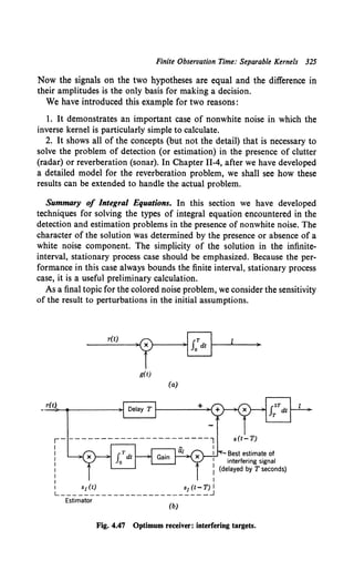
343. Sensitivity 327
In other words, it is a delayed version of the desired signal. Let the actual
interference signal be
s1,.(t) = s(t - T - Lh). (319)
Find tl.dfd as a function of llT.
These examples illustrate typical parameter variation problems. Clearly,
the appropriate variations depend on the physical problem of interest.
In almost all of them the succeeding calculations are straightforward.
Some typical cases are included in the problems.
The functional variation approach is more interesting. As before, we do
a "worst-case" analysis. Two examples are the following:
1. Let the actual signal be
s,.(t) = v'Es(t) + ...;x;s.(t), (320)
where
(321)
To find the worst case we choose s.(t) to make lld as negative as possible.
2. Let the actual noise be
n,.(t) = n(t) + n.(t)
whose covariance function is
K,.,.(t, u) = K,.(t, u) + K,..(t, u),
We assume that n.(t) has finite energy in the interval
This implies that
Tr
IIK,..2(t, u) dt du ~ tl.,..
Tl
(322a)
(322b)
(323a)
(323b)
To find the worst case we choose K,..(t, u) to make lld as negative as
possible.
Various other perturbations and constraints are also possible. We now
consider a simple version of the first problem. The second problem is
developed in detail in [42].
We assume that the noise process is stationary with a spectrum S,.(w)
and that the observation interval is infinite. The optimum receiver, using
a whitening realization (see Fig. 4.38a), is shown in Fig. 4.48a. The

344. 328 4.3 Detection and Estimation in Nonwhite Gaussian Noise
r(t)
{ Nominal output
r.(t)=s.(t) +n.(t)
E(liHo)
E(liHo)
(a)
1'2
(b)
(c)
....fEs(t)
Decision line
Var !liH0)=d2
Decision line
Fig. 4.48 Sensitivity analysis: (a) filter with nominal input; (b) nominal decision space;
(c) actual design space.

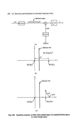
345. Sensitivity 329
corresponding decision space is shown in Fig. 4.48b. The nominal per-
formance is
d _ E(IIH1) - E(liHa) _
- [Var (/jH0)]Yz -
s:"' s!(t) dt
[JCX) ]y,'
-oo s!(t)dt
2
(324)
or
(325)
We let the actual signal be
Sa(t) = VEs(t) + VE. S,(t), -00 < t < oo, (326)
where s(t) and s,(t) have unit energy. The output of the whitening filter
will be
-00 < t < oo, (327)
and the decision space will be as shown in Fig. 4.48c. The only quantity
that changes is E(laiH1). The variance is still the same because the noise
covariance is unchanged. Thus
(328)
To examine the sensitivity we want to make !1d as negative as possible.
If we can make !1d = - d, then the actual operating characteristic will be
the P0 = PF line which is equivalent to a random test. If !1d < - d, the
actual test will be worse than a random test (see Fig. 2.9a). It is important
to note that the constraint is on the energy in s.(t), not s*,(t). Using
Parseval's theorem, we can write (328) as
(329)
This equation can be written in terms ofthe original quantities by observing
that
and
Thus
!1d = v'~E, J_CX)CX) ~: S,Uw)IHwUw)i 2 S*(jw)
_ VEE, foo S Uw) S*(jw) dw.
- d _00 • Sn(w) 27T
(330)
(331)
(332)

346. 330 4.3 Detection and Estimation in Nonwhite Gaussian Noise
The constraint in (321) can be written as
I"' ISE(jw)l2 d
2w = 1.
-"' 11'
(333)
To perform a worst-case analysis we minimize !l.d subject to the constraint
in (333) by using Lagrange multipliers. Let
(334)
Minimizing with respect to SE(jw), we obtain
S (j) =- ~S(jw)
Eo W 2>..d S,.(w)' (335)
(the subscript o denotes optimum). To evaluate >.. we substitute into the
constraint equation (333) and obtain
EEE I"' IS(jw)l2 dw = l (336)
4>..2d2 _"' S,.2(w) 211' '
Ifthe integral exists, then
2>.. = VEEE [I"' IS(jw)1
2
dw] Yo.
d _"' S,.2(w) 211'
(337)
Substituting into (335) and then (332), we have
(338)
(Observe that we could also obtain (338) by using the Schwarz inequality
in (332).) Using the frequency domain equivalent of (325), we have
{[I"' IS(jw)l2
dw] Yz}
a:~ -(;r rf ~~J::?~·~l ·
-oo S,.(w) 211'
(339)
In the white noise case the term in the brace reduces to one and we
obtain the same result as in (82). When the noise is not white, several
observations are important:
1. Ifthere is a white noise component, both integrals exist and the term
in the braces is greater than or equal to one. (Use the Schwarz inequality
on the denominator.) Thus in the colored noise case a small signal
perturbation may cause a large change in performance.
2. If there is no white noise component and the nominal test is not
singular, the integral in the denominator exists. Without further restrictions

347. Known Linear Channels 331
on SUw) and Sn(w) the integral in the numerator may not exist. If it does
not exist, the above derivation is not valid. In this case we can find an
S(Uw) so that !ld will be less than any desired fldx. Choose
{
k S(jw), win 0,
S£(jw) = Sn(w)
0, w not inn,
(340)
where 0 is a region such that
(341)
and k is chosen to satisfy the energy constraint on s((t). We see that in
the absence of white noise a signal perturbation exists that will make the
test performance arbitrarily bad. Such tests are referred to as unstable (or
infinitely sensitive) tests. We see that stability is a stronger requirement
than nonsingularity and that the white noise assumption guarantees a
nonsingular, stable test. Clearly, even though a test is stable, it may be
extremely sensitive.
3. Similar results can be obtained for a finite interval and nonstationary
processes in terms of the eigenvalues. Specifically, we can show (e.g.,
[42]) that the condition
is necessary and sufficient for stability. This is identical to the condition
for g(t) to be square-integrable.
In this section we have illustrated some of the ideas involved in a
sensitivity analysis of an optimum detection procedure. Although we have
eliminated unstable tests by the white noise assumption, it is still possible
to encounter sensitive tests. In any practical problem it is essential to
check the test sensitivityagainst possibleparameterand function variations.
We can find cases in which the test is too sensitive to be of any practical
value. In these cases we try to design a test that is nominally suboptimum
but less sensitive. Techniques for finding this test depend on the problem
of interest.
Before leaving the colored noise problem we consider briefly a closely
related problem.
4.3.8 Known Linear Channels
There is an almost complete duality between the colored additive noise
problem and the problem of transmitting through a known linear channel
with memory. The latter is shown in Fig. 4.49a.

348. 332 4.3 Detection and Estimation in Nonwhite Gaussian Noise
The received waveform on H1 in the simple binary problem is
IT!
r(t) = hch(t, u)VE s(u)du + w(t),
T,
(342)
This is identical in form to (146). Thus hch(t, u) plays an analogous role
to the whitening filter. The optimum receiver is shown in Fig. 4.49b. The
performance index is
= ~I:' dt u:hch(t, u) s(u) du J:hch(t, v) s(v) dv], (343)
where the limits (a, b) depend on the channel's impulse response and the
input signal duration. We assume that T1 :::;; a :::;; b :::;; T1. We can write
this in a familiar quadratic form:
b
d2 = ~IJdu dv s(u) Qch(u, v) s(v) (344)
a
by defining
IT!
Qch(u, v) = hch(t, u) hch(t, v) dt,
Tt
a:::;; u, v:::;; b. (345)
The only difference is that now Qch(u, v) has the properties of a covariance
function rather than an inverse kernel. A problem of interest is to choose
w(t)
--~)1 hch(t,u) 1-1--~)cbt---+) r(t)
s(t) . . s*(t)
(a)
r(t)
s(t)
(b)
Fig. 4.49 Known dispersive channel.

349. The Composite Hypothesis Problem 333
s(t) to maximize d2• The solution follows directly from our earlier signal
design results (p. 302). We can express d2 in terms of the channel eigen-
values and eigenfunctions
(346)
where
St ~ J: VEs(u) tf>t(u) du (347)
and >.,ch and •Mu) correspond to the kernel Qch(u, v). To maximize d2 we
choose
and (348)
St = 0, i '# 1,
because ..1ch is defined as the largest eigenvalue of the channel kernel
Qoh(u, v). Some typical channels and their optimum signals are developed
in the problems.
When we try to communicate sequences of signals over channels with
memory, another problem arises. Looking at the basic communications
system in Fig. 4.1, we see that inside the basic interval 0 ~ t ~ T there is
interference due to noise and the sequence of signals corresponding to
previous data. This second interference is referred to as the intersymbol
interference and it turns out to be the major disturbance in many systems
of interest. We shall study effective methods of combatting intersymbol
interference in Chapter 11.4.
4.4 SIGNALS WITH UNWANTED PARAMETERS: THE COMPOSITE
HYPOTHESIS PROBLEM
Up to this point in Chapter 4 we have assumed that the signals of
concern were completely known. The only uncertainty was caused by the
additive noise. As we pointed out at the beginning of this chapter, in many
physical problems of interest this assumption is not realistic. One example
occurs in the radar problem. The transmitted signal is a high frequency
pulse that acquires a random phase angle (and perhaps a random ampli-
tude) when it is reflected from the target. Another example arises in the
communications problem in which there is an uncertainty in the oscillator
phase. Both problems are characterized by the presence of an unwanted
parameter.
Unwanted parameters appear in both detection and estimation problems.
Because of the inherent similarities, it is adequate to confine our present

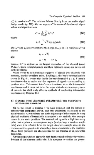
350. 334 4.4 Signals with Unwanted Parameters
discussion to the detection problem. In particular, we shall discuss general
binary detection. In this case the received signals under the two hypotheses
are
r(t) = s1(t, 8) + n(t),
r(t) = s0(t, 8) + n(t),
T1 ~ t ~ T1 :Ht.
~ ~ t ~ T1 :Ho.
(349)
The vector 8 denotes an unwanted vector parameter. The functions s0(t, 8)
and s1(t, 8) are conditionally deterministic (i.e., if the value of 8 were
known, the values of s0(t, 8) and s1(t, 8) would be known for all t in the
observation interval). We see that this problem is just the waveform
counterpart to the classical composite hypothesis testing problem discussed
in Section 2.5. As we pointed out in that section, three types of situations
can develop:
1. 8 is a random variable with a known a priori density;
2. 8 is a random variable with an unknown a priori density;
3. 8 is a nonrandom variable.
We shall confine our discussion here to the first situation. At the end of
the section we comment briefly on the other two. The reason for this choice
is that the two physical problems encountered most frequently in practice
can be modeled by the first case. We discuss them in detail in Sections 4.4.1
and 4.4.2, respectively.
The technique for solving problems in the first category is straight-
forward. We choose a finite set of observables and denote them by the
K-dimensional vector r. We construct the likelihood ratio and then let
K-+ao.
A[r(t)] ~ lim Prl H1 (R!Ht).
K-+«> Pr!Ho(RIHo)
(350)
The only new feature is finding p..1n,(R!Ht) and p..1n0 (RIHo) in the
presence of 8. If 8 were known, we should then have a familiar problem.
Thus an obvious approach is to write
and
Pr!Ho(RIHo) = f Pr!e.n0 (Rj8, Ho) Pelno(81Ho) d8. (352)
Jxe
Substituting (351) and (352) into (350) gives the likelihood ratio. The
tractability of the procedure depends on the form of the functions to be
integrated. In the next two sections we consider two physical problems in
which the procedure leads to easily interpretable results.

351. Random Phase Angles 335
4.4.1 Random Phase Angles
In this section we look at several physical problems in which the un-
certainty in the received signal is due to a random phase angle. The first
problem of interest is a radar problem. The transmitted signal is a band-
pass waveform which may be both amplitude- and phase-modulated. We
can write the transmitted waveform as
()_{V2£;f(t) COS [wet + !fo(t)],
St t -
0,
O~t~T,
elsewhere.
(353)
Two typical waveforms are shown in Fig. 4.50. The function f(t) corre-
sponds to the envelope and is normalized so that the transmitted energy is
E1• The function !fo(t) corresponds to a phase modulation. Both functions
are low frequency in comparison to we.
For the present we assume that we simply want to decide whether a
target is present at a particular range. If a target is present, the signal will
be reflected. In the simplest case of a fixed point target, the received wave-
form will be an attenuated version of the transmitted waveform with a
random phase angle added to the carrier. In addition, there is an additive
white noise component w(t) at the receiver whether the target is present or
f(t) Q>(t)
0
(a)
f(t) Q>(t)
(b)
Fig. 4.50 Typical envelope and phase functions.

352. 336 4.4 Signals with Unwanted Parameters
not. If we define H1 as the hypothesis that the target is present and H0 as
the hypothesis that the target is absent, the following detection problem
results:
H1: r(t) = V2E. /(t - T) COS (w0 (t - T) + rfo(t - T) + 0)
+ w(t), T ::-:; t ::-:; T + T,
= w(t), T1 ::-:; t < T, T + T < t ::-:; T1,
~ Sr(t - T, 0) + w(t),
H0 :r(t) = w(t);
T1 ::-:; t ::-:; T1•
T1 ::-:; t ::-:; T1•
(354a)
(354b)
Because the noise is white, we need only observe over the interval
T ::-:; t ::-:; T + T. Under the assumption that we are interested only in a
particular T, the model is the same if we let T = 0. Thus we need only
consider the problem
H1:r(t) = Sr(t, 0) + w(t),
H0 :r(t) = w(t),
0 ::-:; t ::-:; T,
0 ::-:; t ::-:; T.
(355a)
(355b)
Here we have a simple binary detection problem in which the unknown
parameter occurs only on one hypothesis. Before solving it we indicate
how a similar problem can arise in the communications context.
In a simple on-off communication system we send a signal when the
source output is "one" and nothing when the source output is "zero".
The transmitted signals on the two hypotheses are
H1 :st(t) = V2Et f(t) COS (wet + <fo(t) + 84 ),
Ho:s1(t) = 0,
0 5, t 5, T,
05,t5,T.
(356)
Frequently, we try to indicate to the receiver what 84 is. One method of
doing this is to send an auxiliary signal that contains information about
84 • Ifthis signal were transmitted through a noise-free channel, the receiver
would know 84 exactly and the problem would reduce to the known signal
problem. More frequently the auxiliary signal is corrupted by noise and
the receiver operates on the noise-corrupted auxiliary signal and tries to
estimate 84 • We denote this estimate by 04 • A block diagram is shown in
Fig. 4.51. We discuss the detailed operation of the lower box in Chapter
11.2. Now, if the estimate Da equals 84 , the problem is familiar. If they are
unequal, the uncertainty is contained in the difference 8 = oa - ea. which
is a random variable. Therefore we may consider the problem:
H1 :r(t) = V2Erf(t) cos (w0 t + <fo(t) + 8) + w(t),
H0 :r(t) = w(t),
0 5, t 5, T, (357)
0 5, t ::-:; T, (358)

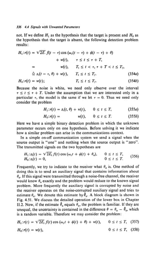
353. Random Phase Angles 337
Data signals
Transmitter 1----~
Auxiliary
signal
(pilot tone)
Fig. 4.51 A pbase estimation system.
where E, is the actual received signal energy and 6 is the phase measure-
ment error. We see that the radar and communication problems lead to the
same mathematical model.
The procedure for finding the likelihood ratio was indicated at the
beginning of Section 4.4. In this particular case the model is so familiar
(see (23)) that we can write down the form for K--+ oo immediately. The
resulting likelihood ratio is
A[r(t)] = J:11
p8(6)d6exp [+;0
J:r(t)s,(t,6)dt- ~oLT s,2(t,6)dt],
(359)
where we assume the range of 6 is [-7T, 7T]. The last integral corresponds
to the received energy. In most cases of interest it will not be a function of
the phase so we incorporate it in the threshold. To evaluate the other
integral, we expand the cosine term in (357),
cos [wet + ~(t) + 6] = cos [wet+ ~(t)] cos 6- sin [wet+ ~(t)] sin 6, (360)
and define
Le Q LT v'2 r(t) f(t) COS [wet + ~{t)) dt, (361)
and
Ls Q LT v2r(t) f(t) sin [wet + ~(t)] dt. (362)
Thus the integral of interest is
In: [2vE ]
A'[r(t)] = -n: p8(6) d6 exp Nor (Lc cos 6- L8 sin 6) . (363)
To proceed we must specify p8(8). Instead ofchoosing a particular density,
we specify a family of densities indexed by a single parameter. We want to
choose a family that will enable us to model as many cases of interest as

354. 338 4.4 Signals with Unwanted Parameters
1.2
1.1
1.0
0.9
t
0.8
,......
0.7
e
< Symmetric about 9=0
~
~ 0.6
0.5
0.4
0.3
0.2
0.1
,_
Fig. 4.52 Family of probability densities for the phase angle.
possible. A family that will turn out to be useful is given in (364) and shown
in Fig. 4.52t:
(8.A ) ~ exp [Am cos 8).
PB . m 271' fo(Am) '
-71' ~ 8 ~ 71', (364)
The function /0(Am) is a modified Bessel function of the first kind which
is included so that the density will integrate to unity. For the present Am
t This density was first used ior this application by Viterbi [44].

355. Random Phase Angles 339
can be regarded simply as a parameter that controls the spread of the
density. When we study phase estimators in Chapter 11.2, we shall find
that it has an important physical significance.
Looking at Fig. 4.52, we see that for Am = 0
Pe(8) = 2~, -Tr ~ 8 ~ Tr. (365)
This is the logical density for the radar problem. As Am increases, the
density becomes more peaked. Finally, as Am~ oo, we approach the known
signal case. Thus by varying Am we can move continuously from the
known signal problem through the intermediate case, in which there is
some information about the phase, to the other extreme, the uniform
phase problem.
Substituting {364) into (363), we have
A'[r{t)] = rn21T /:(Am) exp [(Am+ 2~~rLc) cos 8- 2~~rL.sin 8] d8.
(366)
This is a standard integral (e.g., [45]). Thus
, 1 {[( 2V£, )2 (2v'£, )2]%}
A [r(t)] = lo(Am) lo Am + ~ Lc + ~ L. · (367)
Substituting (367) into (359), incorporating the threshold, and taking the
logarithm, we obtain
Hl E
~ ln 7J + 11.rr + ln /0(Am)· (368)
Ho lYo
The formation of the test statistic is straightforward (Fig. 4.53). The
function /0( ·) is shown in Fig. 4.54. For large x
whereas for small x
and
e"'
/ 0(x) ~. 1- •
V 21TX
x2
10(x) ~ 1 + 4'
x2
ln /0(x) ~ 4 ,
X» 1, (369)
X« 1, (370a)
X« 1. (370b)
Observe that because ln /0(x) is monotone we can remove it by modifying

356. 340 4.4 Signals with Unwanted Parameters
-../2.f(t) sin [wet+ rp(t)]
Fig. 4.53 Optimum receiver: random phase angle
the threshold. Thus two tests equivalent to (368) are
( N
0Am)2
2 ~1
Lc + 2V£; + L. !fay (37la)
and
(2VEr)2
(L 2 + L 2) + 2A 2VEr L ~ '
AT C S m AT C < ')' '
lYQ lYQ Ho
(37Ib)
t
1~~-L----~--~--~----~--~--~
0 1.0 2.0 3.0 4.0 5.0 6.0
X~
Fig. 4.54 Plot of lo(x).

357. Matched Filter-Envelope Detector 341
Linear component
r---------,
I I
I I
I I
I I
L_ .J
.../ff(t) sin (wet+ tf>(t))
Fig. 4.55 Alternate realization of optimum receiver.
Redrawing the receiver structure as shown in Fig. 4.55, we see that the
optimum receiver consists of a linear component and a square-law
component.
Looking at (371a), we see that the region in the L 0 , L. plane corre-
sponding to the decision H0 is the interior of a circle centered at
( -N0Amf2VJI;, 0) with radius yYz. We denote this region as n0• The
probability density of Lc and L. under H0 is a circularly symmetric
Gaussian density centered at the origin. Therefore, if y is fixed and Am is
allowed to increase, no will move to the left and the probability of being
in it on H0 will decrease. Thus, to maintain a constant PF we increase y as
Am is increased. Several decision regions are shown in Fig. 4.56. In the
limit, as Am ~ oo, the decision boundary approaches a straight line and
we have the familiar known signal problem of Section 4.2. The probability
density on H1 depends on 8. A typical case is shown in the figure. We
evaluate PF and Pv for some interesting special cases on p. 344 and in the
problems. Before doing this it will be worthwhile to develop an alternate
receiver realization for the case in which Am = 0. In many cases this
alternate realization will be more convenient to implement.
Matched Filter-Envelope Detector Realization. When Am = 0, we must
find VL0
2 + L,2 • We can do so by using a bandpass filter followed by an
envelope detector, as shown in Fig. 4.57. Because h(t) is the impulse
response of a bandpass filter, it is convenient to write it as
(372)

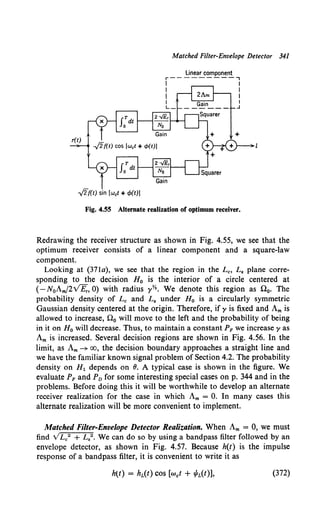
358. 342 4.4 Signals with Unwanted Parameters
Equal contour lines for
PL••L.IH1,6(Lc,LsiH1,9)
No
atLc=---Am
2-../E,.
nl = no is region of
plane outside circle
Fig. 4.56 Decision regions, partially coherent case.
Lc
where hL(t) and •h(t) are low-pass functions. The output at time Tis
y(n = s:h(T- 'T) r('T) d'T. (373)
Using (372), we can write this equation as
y(n = J:r(T) hL(T- 'T) cos [wc(T- 'T) + •h(T- 'T)] d'T
= cos w0 T IoT r(T) hL(T- 'T) cos [r.oc'T - rfiL(T- T)] d'T
+ sin weT J:r(T) hL(T - T) sin [weT - rfL(T- T)] dT. (374)
r(t)
Bandpass
filter
Observe at time
~ t=T
~-----
Fig. 4.57 Matched filter-envelope detector for uniform phase case.

359. Random Phase 343
This can be written as
y(T) ~ Yc(T) COS weT + y.(T) sin weT
= Vye2(T) + Ys2(T) cos [weT - tan-l ~:~~] • (375)
Observing that
Yc(T) = Re J:r(T) hL(T- T) exp [+jw0 T- jt/JL(T- T)] dT (376a)
and
y.(T) = Im J:r(T) hL(T- T) exp [+jw0 T - j!fL(T- T)] dT, (376b)
we see that the output of the envelope detector is
Vyc2(T) + y.2(T) =II: r(T) hL(T- T) exp [-jt/JL(T- T) + jW0 T] dTI·
(377)
From (361) and (362) we see that the desired test statistic is
VL0
2 + L8
2 = IJ:r(T)Vlj(T)e+ld><•>e+lm.• d+ (378)
We see the two expressions will be identical if
and
hL(T- T) = Vlf(T)
tPL(T- T) = -rp(T).
(379)
(380)
This bandpass matched filter provides a simpler realization for the uniform
phase case.
The receiver in the uniform phase case is frequently called an incoherent
receiver, but the terminology tends to be misleading. We see that the
matched filter utilizes all the internal phase structure of the signal. The
only thing missing is an absolute phase reference. The receiver for the
known signal case is called a coherent receiver because it requires an
oscillator at the receiver that is coherent with the transmitter oscillator.
The general case developed in this section may be termed the partially
coherent case.
To complete our discussion we consider the performance for some
simple cases. There is no conceptual difficulty in evaluating the error
probabilities but the resulting integrals often cannot be evaluated analyti-
cally. Because various modifications of this particular problem are fre-
quently encountered in both radar and communications, a great deal of
effort has been expended in finding convenient closed-form expressions

360. 344 4.4 Signals with Unwanted Parameters
and in numerical evaluations. We have chosen two typical examples to
illustrate the techniques employed.
First we consider the radar problem defined at the beginning of this
section (354-355).
Example 1 (Uniform Phase). Because this model corresponds to a radar problem, the
uniform phase assumption is most realistic. To construct the ROC we must compute
PF and Po. (Recall that PFand Po are the probabilities that we will exceed the threshold
, when noise only and signal plus noise are present, respectively.)
Looking at Fig. 4.55, we see that the test statistic is
(381)
where Lc and L, are Gaussian random variables. The decision region is shown in
Fig. 4.56. We can easily verify that
Ho:E(Lc) = E(L,) = 0; Var(Lc) = Var(L,) = ~o,
_,- _,- No
H1 : E(Lcl8) = v E, cos 8; E(L,IB) = v E, sin 8; Var (Lc) = Var (L,) = 2 · (382)
Then
II( N)-1
( L2
+L")
PF ~ Pr [/ > YIHo] = 21T 2° exp - c No • dLc dL,. (383)
no
Changing to polar coordinates and evaluating, we have
PF = exp ( -~J (384)
Similarly, the probability of detection for a particular 8 is
Po(8) = II(2.,. ~0r1 exp (-(Lc - v'E,cos 8)2~ (L, - v'E,sin 8)2) dLc dL,. (385)
iio
Letting Lc = R cos {3, L, = R sin /3, and performing the integration with respect to {3,
we obtain
f., 2 ( R2 + E,) (2Rv'E,)
Po({/) = Po = ../v NoR exp -~ Io ~ dR. (386)
As we expected, Po does not depend on 8. We can normalize this expression by letting
z = V2/N0 R. This gives
1
., ( z2 + d2)
Po = _ z exp ---
2- l 0(zd) dz,
../2>/No
(387)
where d2 Q 2E,/No.
This integral cannot be evaluated analytically. It was first tabulated by Marcum
[46, 48] in terms of a function commonly called Marcum's Q function:
f"" ( z2
+ a 2
)
Q(a, {3) ~ J6
z exp ---
2- l 0(az) dz. (388)
This function has been studied extensively and tabulated for various values of a, {3
(e.g., [48], [49], and [SO]). Thus
( (2,)%
Po= Q d, No · (389)

361. Random Phase 345
i
0.4
0.2
0 .......
0
.......................
...···
...···
.·
...............
d= fiE;
VN;
1.0
Fig. 4.58 Receiver operating characteristic, random phase with uniform density.
This can be written in terms of Pp. Using (384), we have
PD = Q(d, v -2ln Pp). (390)
The ROC is shown in Fig. 4.58. The results can also be plotted in the form of PD
versus d with PF as a parameter. This is done in Fig. 4.59. Comparing Figs. 4.14 and
4.59, we see that a negligible increase of dis required to maintain the same Pn for a
fixed PF when we go from the known signal model to the uniform phase model for
the parameter ranges shown in Fig. 4.59.
The second example of interest is a binary communication system in
which some phase information is available.
Example 2. Partially Coherent Binary Communication. The criterion is minimum
probability of error and the hypotheses are equally likely. We assume that the signals
under the two hypotheses are
H1 :r(t) = V2E,fl(t)cos(wct + 8) + w(t),
H 0 :r(t) = V2E,f0(t)cos(wct + 8) + w(t),
0:5;t:5;T,
0 :5; t :5; T,
(391)

362. 346 4.4 Signals with Unwanted Parameters
where / 0(1) and / 1(1) are normalized and
f/o(l) /1(t) dt = p; -l:S:p:S:l. (392)
The noise spectral height is N0 /2 and p6(1J) is given by (364). The likelihood ratio test
is obtained by an obvious modification of the simple binary problem and the receiver
structure is shown in Fig. 4.60.
We now look at Pr (•) as a function of p, d2 , and Am. Intuitively, we expect that as
Am-+ oo we would approach the known signal problem, and p = -1 (the equal and
opposite signals of (39)) would give the best result. On the other hand, as Am -+ 0,
t
d=- (Jff;_ ~
YHO
Fig. 4.59 Probability of detection vs d, uniform phase.

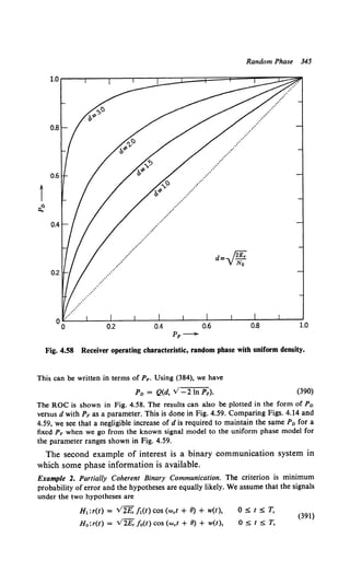
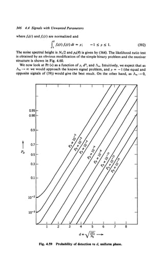
363. Random Phase 347
Linear component
r-- --------,
I I
I I
I
I
I
...__
r(t)
2[fl(t)) sin(w0t)
r(t)
r(t)
2[fo(t)] sin(wct)
Fig. 4.60 Receiver: binary communication system.
the phase becomes uniform. Now, any correlation (+ or -) would move the signal
points closer together. Thus, we expect that p = 0 would give the best performance.
As we go from the first extreme to the second, the best value of p should move from
-1 to 0.
We shall do only the details for the easy case in which p = -1; p = 0 is done in
Problem 4.4.9. The error calculation for arbitrary p is done in [44].
When p = - 1, we observe that the output of the square-law section is identical
on both hypotheses. Thus the receiver is linear. The effect of the phase error is to
rotate the signal points in the decision space as shown in Fig. 4.61.
Using the results of Section 4.2.1 (p. 257),
p ( !B) fo (2 No) -y, [ (x - v£,. cos 8)2
] d
r € = _"' ,. T exp - No X (393)

364. 348 4.4 Signals with Unwanted Parameters
y
Fig. 4.61 Eft'ect of phase errors in decision space.
or
I-..;2E,INo co• e 1 ( z2)
Pr (£18) = _"' v'2, exp -2 dz. (394)
Using (364),
Pr (£) = J+"exp (Am cos 8) Pr (£IB) dB.
_, 2wlo(Am)
(395)
This can be integrated numerically. The results for two particular values of d2 are
shown in Figs. 4.62 and 4.63.t The results for other p were also evaluated in [44]
and are given in these figures. We see that for Am greater than about 2 the negatively
correlated signals become more efficient than orthogonal signals. For Am ~ 10 the
difference is significant. The physical significance of Am will become clearer when we
study phase estimating systems in Chapter 11.2.
In this section we have studied a particular case of an unwanted param-
eter, a random phase angle. By using a family of densities we were able to
demonstrate how to progress smoothly from the known signal case to the
uniform phase case. The receiver consisted of a weighted sum of a linear
operation and a quadratic operation. We observe that the specific receiver
structure is due to the precise form of the density chosen. In many cases
the probability density for the phase angle would not correspond to any
of these densities. Intuitively we expect that the receiver developed here
should be "almost" optimum for any single-peaked density with the same
variance as the member of the family for which it was designed.
We now turn to a case of equal (or perhaps greater) importance in
which both the amplitude and phase of the received signal vary.
t The values of d2 were chosen to give aPr(£)= lQ- 3 and lQ- 5, respectively, at
Am= CO,

365. Random Phase 349
10°~------------~----------~~----------~
t
Pr(E)
(d =3.098)
Fig. 4.62 Pr (€}, partially coherent binary system (lQ- 3 asymptote} [44].
4.4.2 Random Amplitude and Phase
As we discussed in Section 4.1, there are cases in which both the
amplitude and phase of the received signal vary. In the communication
context this situation is encountered in ionospheric links operating above
the maximum usable frequency (e.g., [51]) and in some tropospheric links
(e.g., [52]). In the radar context it is encountered when the target's aspect
or effective radar cross section changes from pulse to pulse (e.g., Swerling
[53]).
Experimental results for a number of physical problems indicate that
when the input is a sine wave, v'2 sin w.t, the output (in the absence of
additive noise) is
(396)
An exaggerated sketch is shown in Fig. 4.64a. The envelope and phase
vary continuously. The envelope vch(t) has the Rayleigh probability
density shown in Fig. 4.64b and that the phase angle Bch(t) has a uniform
density.

366. 350 4.4 Signals with Unwanted Parameters
10°r-------------r-------------r-----------~
t
Pr(E)
(d =4.265)
10 100
Am-
Fig. 4.63 Pr (£),partially coherent binary system (lo-s asymptote) [44].
There are several ways to model this channel. The simplest technique is
to replace the actual channel functions by piecewise constant functions
(Fig. 4.65). This would be valid when the channel does not varysignificantly

367. (a)
Pu(:)
Fig. 4.64 Narrow-band process at output of channel, and the probability of Its
envelope.
V(t)
(a)
(b)
Fig. 4.65 Piecewise constant approximation: (a) actual envelope; (b) piecewise
constant model.
351

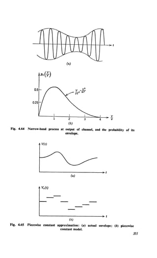
368. 352 4.4 Signals with Unwanted Parameters
in a T second interval. Given this "slow-fading" model, two choices are
available. We can process each signaling interval independently or exploit
the channel continuity by measuring the channel and using the measure-
ments in the receiver. We now explore the first alternative.
For the simple binary detection problem in additive white Gaussian
noise we may write the received signal under the two hypotheses ast
H1 :r(t) = vVlf(t)cos [wet+ r/>(t) + 8] + w(t),
H0 :r(t) = w(t),
0 :5 t :5 T, (397)
0:5t:5T,
where v is a Rayleigh random variable and 8is a uniform random variable.
We can write the signal component equally well in terms of its quad-
rature components:
V2 v f(t) cos [wet + r/>(t) + 8] = alv2 f(t) cos [wet + r/>(t)]
+ a2 v'2 f(t) sin [wet + r/>(t)],
0 :5 t :5 T, (398)
where a1 and a2 are independent zero-mean Gaussian random variables
with variance a2 (where E[v2] = 2a2; see pp. 158-161 of Davenport and
Root [2]). We also observe that the two terms are orthogonal. Thus the
signal out of a Rayleigh fading channel can be viewed as the sum of two
orthogonal signals, each multiplied by an independent Gaussian random
variable. This seems to be an easier way to look at the problem. As a
matter of fact, it is just as easy to solve the more general problem inwhich
the received waveform on H1 is,
M
r(t) = L a1 s1(t) + w(t), 0:5t:5T, (399)
I= 1
where the a1 are independent, zero-mean Gaussian variables N(O, a..) and
(400)
The likelihood ratio is
A[r(t)] =
J~oo···J~oop..JAl) p...(A2) · · ·PaM(AM) exp [ +; 0J:r(t) 1~ A1s1(t) dt
~
(401)
t For simplicity we assume that the transmitted signal has unit energy and adjust the
received energy by changing the characteristics of v.

369. Rayleigh Channels 353
r(t)
(a)
(b)
Fig. 4.66 Receivers for Gaussian amplitude signals: (a) correlation-squarer receiver;
(b) filter-squarer receiver.
Defining
(402)
using the orthogonality of the s1(t), and completing the square in each of
the M integrals, we find the test reduces to
l /::;,L2 a, >
M ( a 2 ) H1
- £... I 2 < ')'.
1=1 C1a1 + No/2 Ho
(403)t
Two receivers corresponding to (403) and shown in Fig. 4.66 are commonly
called a correlator-squarer receiver and a filter-squarer receiver, respec-
tively. Equation 403 can be rewritten as
M ( a 2L ) M
I = LL, 2 a, lv: /2 = LL/i,.
1=1 aa, + 0 1=1
(404)
t Note that we could have also obtained (403) by observing that the L, are jointly
Gaussian on both hypotheses and are sufficient statistics. Thus the results of Section
2.6 [specifically (2.326)] are directly applicable. Whenever the L, have nonzero means
or are correlated, the use of 2.326 is the simplest method (e.g., Problem 4.4.21).

370. 354 4.4 Signals with Unwanted Parameters
This structure, shown in Fig. 4.67, can be interpreted as an estimator-
correlator receiver (i.e., we are correlating r(t) with our estimate of the
received signal.) The identification of the term in braces as a
1 follows from
our estimation discussion in Section 4.2. It is both a minimum mean-square
error estimate and a maximum a posteriori probability estimate. In Fig.
4.67a we show a practical implementation. The realization in Fig. 4.67b
shows that we could actually obtain the estimate of the signal component
as a waveform in the optimum receiver. This interpretation is quite
important in later applications.
r(t)
r(t)
(a)
BM(t- T)
(b)
Fig. 4.67 Estimator-correlator receiver.
MMSE estimate
of signal
component

371. Rayleigh Channels 355
We now apply these results to the original problem in (397). If we relate
L1 to Lc and L2 to L., we see that the receiver is
(405)
(where Lc and L. were defined in the random phase example). This can be
realized, as shown in the preceding section, by a bandpass matched filter
followed by an envelope detector. The two alternate receiver realizations
are shown in Figs. 4.68a and b.
The next step is to evaluate the performance. We observe that Lc and L.
are Gaussian random variables with identical distributions. Thus the
Rayleigh channel corresponds exactly to Example 2 on p. 41 of Chapter 2.
In Equation (2.80), we showed that
Pn = {PF)"o21"12 , {2.80}
where a02 is the variance of Lc on H0 and a12 is the variance of Lc on H1•
Looking at Fig. 4.58a, we see that
No
a 02 = 2 (406)
and
2 No 2 E 6. No E,
(11 = T + (1 I - T + 2' (407)
where E, ~ 2a2 E1 is the average received signal energy
r(t)
(a)
r(t)
h(T)=-¥2f(T-T)COS(WcT- (jJ(T- T))
(b)
Fig. 4.68 Optimum receivers, Rayleigh channel: (a) squarer realization; (b) matched
filter-envelope detector realization.

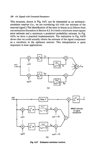
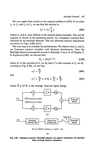
372. 356 4.4 Signals with Unwanted Parameters
because v2 is the received signal energy. Substituting (406) and (407) into
(2.80), we obtain
PF = (Pv)l+ E,tNo (408)
The ROC is plotted in Fig. 4.69.
The solution to the analogous binary communication problem for
arbitrary signals follows in a similar fashion (e.g., Masonson [55] and
0.8
0.7
t
0.1 0.2 0.3 0.4 0.5
PF~
Fig. 4.69 (a) Receiver operating characteristic, Rayleigh channel.
Turin [56]). We discuss a typical system briefly. Recall thatthe phaseangle
8 has a uniform density. From our results in the preceding section (Figs.
4.62 and 4.63) we would expect that orthogonal signals would be optimum.
We discuss briefly a simple FSK system using orthogonal signals. The
received signals under the two hypotheses are
H1 :r(t) = v2 vf(t) cos [w1t + c/>(t) + 8] + w(t),
H0 :r(t) = V2 v f(t) cos [w0t + cfo(t) + 8] + w(t},
O~t~T.
05.t5.T.
(409)

373. Rayleigh Channels 357
The frequencies are separated enough to guarantee orthogonality. Assum-
ing equal a priori probabilities and a minimum probability of error
criterion, 7J = 1. The likelihood ratio test follows directly (see Problem
4.4.24).
2Er --+
No
30
Fig. 4.69 (b) probability of detection vs. 2E,/No.
(410)
50 100
The receiver structure is shown in Fig. 4.70. The probability of error
can be evaluated analytically:
1[ 1£]-l
Pr (E) = - 1 + - __!. •
2 2 N0
(411)
(See Problem 4.4.24.) In Fig. 4.71 we have plotted the Pr (•;) as a function
of E,/N0 • For purposes of comparison we have also shown the Pr (E) for

374. 358 4.4 Signals with Unwanted Parameters
r(t)
Bandpass
matched
filter
Bandpass
matched
filter
Square law
envelope
detector
Square law
envelope
detector
Fig. 4.70 Optimum receiver: binary communication system with orthogonal signals.
the known signal case and the uniform random phase case. We see that
for both nonfading cases the probability of error decreases exponentially
for large E,/N0 , whereas the fading case decreases only linearly. This is
intuitively logical. Regardless of how large the average received energy
becomes, during a deep signal fade the probability of error is equal or
nearly equal to t. Even though this does not occur often, its occurrence
keeps the probability of error from improving exponentially. In Chapter
II.3 we shall find that by using diversity (for example, sending the signal
over several independent Rayleigh channels in parallel) we can achieve an
exponential decrease.
As we have already pointed out, an alternate approach is to measure
the channel characteristics and use this measurement in the receiver
structure. We can easily obtain an estimate of the possible improvement
available by assuming that the channel measurement is perfect. If the
measurement is perfect, we can use a coherent receiver. The resulting Pr (t)
is easy to evaluate. First we write the error probability conditioned on the
channel variable v being equal to V. We then average over the Rayleigh
density in Fig. 4.64b. Using coherent or known signal reception and
orthogonal signals the probability of error for a given value Vis given by
(36) and (40),
and
V -V2 /2a•
2e '
p.,(V) =a
0,
v ~ 0,
v < 0.
(V ~ 0) (412)
(413)

375. Rayleigh Channels 359
Thus
Changing to polar coordinates and integrating, we obtain
(415)
The result is shown in Fig. 4.72.
t
Pr{e)
1o-5 ~~--~~~--~-J--~-J--~~--~~--~~
0 2 3 4 5 6 7 8 9 10 11 12
E,fNo ___,..
Fig. 4.71 Probability of error, binary orthogonal signals, Rayleigh channel.

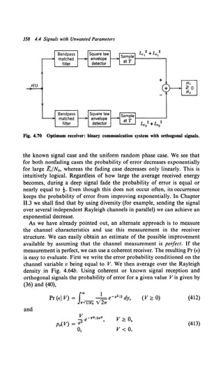
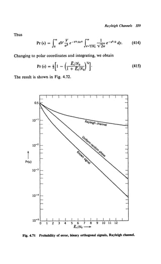
376. 360 4.4 Signals with Unwanted Parameters
Comparing (415) and (411) (or looking at Fig. 4.72), we see that perfect
measurement gives about a 3-db improvement for high E,fN0 values and
orthogonal signals. In addition, if we measured the channel, we could use
equal-and-opposite signals to obtain another 3 db.
Rician Channel In many physical channels there is a fixed (or
"specular") component in addition to the Rayleigh component. A typical
example is an ionospheric radio link operated below the maximum usable
frequency (e.g., [57], [58], or [59]). Such channels are called Rician
channels. We now illustrate the behavior of this type of channel for a
t
Pr(E)
Fig. 4.72 Probability of error, Rayleigh channel with perfect measurement.

377. Rician Channels 361
binary communication system, using orthogonal signals. The received
signals on the two hypotheses are
H1:r(t) = v2 a / 1(t) cos [wet + t/>1(t) + S]
+ V2 Vf1(t) COS [wet + t/>1(t) + 8] + w(t),
O~t~T.
H0 : r(t) = v2 a f 0(t) cos [wet + t/>0(t) + S]
(416)
+ v2 v fo(t) cos [wet + t/>o(t) + 8] + w(t),
O~t~T.
where a and S are the amplitude and phase of the specular component.
The transmitted signals are orthonormal. In the simplest case a and ll are
assumed to be known (see Problem 4.5.26 for unknown S). Under this
assumption, with no loss in generality, we can let 8 = 0. We may now
write the signal component on H1 as
al{v2 _t;(t) cos [wet + tPt(t)]} + a2{v2_t;(t) sin [wet + tf>t(t)]},
(i = 0, 1). (417)
Once again, a1 and a2 are independent Gaussian random variables:
E(a1) = a, E(a2) = 0,
Var (a1) = Var (a2) = a2.
(418)
The expected value of the received energy in the signal component on
either hypothesis is
(419)
where y2 is twice the ratio of the energy in the specular component to the
average energy in the random component.
If we denote the total received amplitude and phase angle as
(420)
The density of the normalized envelope (V~ = V/a)Pv;.(X) and the density
of the phase angle p8.(8') are shown in Fig. 4.73 ([60] and [56]). As we
would expect, the phase angle probability density becomes quite peaked
as y increases.
The receiver structure is obtained by a straightforward modification of
(398) to (405). The likelihood ratio test is

378. ....
~
0.7r----------.-----------.----------,-----------.----------.-----------r----------,
t 0.4
Pv'n(X)
7
x-
Fig. 4.73 (a) Probability density for envelope, Rician channel.

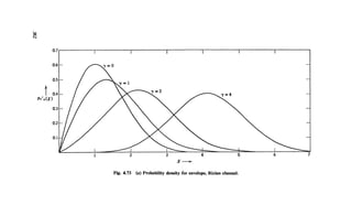
379. Rician Channels 363
1.6
1.5
1.3
1.2
1.1
0.17!" 0.27r 0.37r 0.47r 0.57r 0.67r 0.77r 0.87r 0.97r l.07r
o'
Fig. 4.73 (b) probability density for phase angle, Rician channel.
The receiver structure is shown in Fig. 4.74. The calculation of the
error probability is tedious (e.g., [56]), but the result is
[ y y(f3 + 1) ]
Pr (€) = Q (f3 + !)Yzf3Yz' ({3 + 2)Y.f3Y•
- (~! ~) exp [ _Y;(!32
{3~ ~2; 2)]/o[r2 {3~: ~)] (422)

380. 364 4.4 Signals with Unwanted Parameters
r(t)
-./2fo(t) sin (wet + t/>o(t)]
Fig. 4.74 Optimum receiver for binary communication over a Rician channel.
where fJ f2 2a2/N0 is the expected value of the received signal energy in
the random component divided by N0 • The probability of error is plotted
for typical values of y in Fig. 4.75. Observe that y = 0 is the Rayleigh
channel and y = oo is the completely known signal. We see that even
when the power in the specular component is twice that of the random
component the performance lies close to the Rayleigh channel perform-
ance. Once again, because the Rician channel is a channel of practical
importance, considerable effort has been devoted to studying its error
behavior under various conditions (e.g., [56]).
Summary As we would expect, the formulation for the M-ary signaling
problem is straightforward. Probability of error calculations are once
again involved (e.g., [61] or [15]). In Chapter 11.3 we shall see that both
the Rayleigh and Rician channels are special cases of the general Gaussian
problem.
In this section we have studied in detail two important cases in which
unwanted random parameters are contained in the signal components.

381. Rician Channels 365
Because the probability density was known, the optimum test procedure
followed .directly from our general likelihood ratio formulation. The
particular examples of densities we considered gave integrals that could be
evaluated analytically and consequently led to explicit receiver structures.
Even when we could not evaluate the integrals, the method of setting up
the likelihood ratio was clear.
When the probability density of 8 is unknown, the best procedure is
not obvious. There are two logical possibilities:
1. We can hypothesize a density and use it as if it were correct. We can
investigate the dependence of the performance on the assumed density by
using sensitivity analysis techniques analogous to those we have demon-
strated for other problems.
2. We can use a minimax procedure. This is conceptually straight-
forward. For example, in a binary communication problem we find the
t
Pr(E)
Fig. 4.75 Probability of error for binary orthogonal signals, Rician channel.

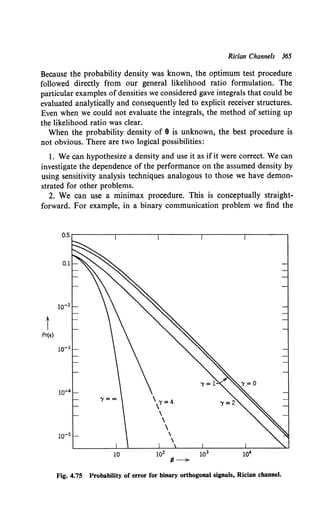
382. 366 4.5 Multiple Channels
Pr (E) as a function of pe(O) and then choose the Pe(O) that maximizes
Pr (E) and design for this case. The two objections to this procedure are its
difficulty and the conservative result.
The final possibility is for 8 to be a nonrandom variable. To deal with
this problem we simply extend the composite hypothesis testing techniques
that we developed in Section 2.5 to include waveform observations. The
techniques are straightforward. Fortunately, in many cases of practical
importance either a UMP test will exist or a generalized likelihood ratio
test will give satisfactory results. Some interesting examples are discussed
in the problems. Helstrom [14] discusses the application of generalized
likelihood ratio tests to the radar problem of detecting signals ofunknown
arrival time.
4.5 MULTIPLE CHANNELS
In Chapter 3 we introduced the idea of a vector random process. We
now want to solve the detection and estimation problems for the case in
which the received waveform is a sample function from a vector random
process.
In the simple binary detection problem, the received waveforms are
H1:r(t) = s(t) + n(t),
H0 :r(t) = n(t),
Tt :S t :S T1,
T1 :S t :S T1•
In the estimation case, the received waveform is
r(t) = s(t, A) + n(t),
Two issues are involved in the vector case:
(423)t
(424)
I. The first is a compact formulation of the problem. By using the
vector Karhunen-Loeve expansion with scalar coefficients introduced in
Chapter 3 we show that the construction of the likelihood ratio is a trivial
extension of the scalar case. (This problem has been discussed in great
detail by Wolf [63] and Thomas and Wong [64].)
2. The second is to study the performance of the resulting receiver
structures to see whether problems appear that did not occur in the scalar
case. We discuss only a few simple examples in this section. In Chapter 11.5
we return to the multidimensional problem and investigate some of the
interesting phenomena.
t In the scalar case we wrote the signal energy separately and worked with normalized
waveforms. In the vector case this complicates the notation needlessly, and we use
unnormalized waveforms.

383. Formulation 367
4.5.1 Formulation
We assume that s(t) is a known vector signal. The additive noise n(t) is
a sample function from an M-dimensional Gaussian random process. We
assume that it contains a white noise component:
where
n(t) = w(t) + Dc(t),
N,
E[w(t)wT(u)] = 2°I 8(t - u).
a more general case is,
E[w(t) wT(u)] = N 8(t - u).
(425)
(426a)
(426b)
The matrix N contains only numbers. We assume that it is positive-
definite. Physically this means that all components of r(t) or any linear
transformation of r(t) will contain a white noise component. The general
case is done in Problem 4.5.2. We consider the case described by (426a) in
the text. The covariance function matrix of the colored noise is
(427)
We assume that each element in Kc(t, u) is square-integrable and that the
white and colored components are independent. Using (425-427), we have
Kn(t, u) = ~0 I 8(t - u) + Kc(t, u). (428)
To construct the likelihood ratio we proceed as in the scalar case.
Under hypothesis H 1
r1 ~ IT1
rT(t) cp1(t) dt
T;
= IT1
sT(t) cp1(t) dt + IT' nT(t) cp1(t) dt
Tt Tt
= s1 + n1• (429)
Notice that all of the coefficients are scalars. Thus (180) is directly
applicable:
"' R1s1 I "' s12
ln A[r(t)] = 2:--- 2: -·
t=l A; 2 t=l A;
(430)
Substituting (429) into (430), we have
TJ
ln A[r(t)] = JJrT(t) 1~ cp;(t):?(u) s(u) dt du
Tt
Tr
- t JJsT(t) 1~ cp,(t):?(u) s(u) dt du. (431)
Tt

384. 368 4.5 Multiple Channels
Defining
1j < t, u < T1, (432)
we have
Tt
In A[r(t)] = ffrT(t) Qn(t, u) s(u) dt du
Tt
Tf
- t ffsT(t) Qn(t, u) s(u) dt du. (433)
Tt
Using the vector form of Mercer's theorem (2.253) and (432), we observe
that
ITt
K0 (t, u) Q0 (u, z) du = S(t - z)I,
T,
(434)
By analogy with the scalar case we write
2
Qn(t, u) = No I[S(t - u) - h0(t, u)] (435)
and show that h0 (t, u) can be represented by a convergent series. The
details are in Problems 4.5.1. As in the scalar case, we simplify (433) by
defining,
IT!
g(t) = Q0 (t, u) s(u) du,
Tt
(436)
r(t) Ht or Ho
g(t)
(a)
r(!!~l T I
=-~g (T-T)I-----'
(b)
Fig. 4.76 Vector receivers: (a) matrix correlator; (b) matrix matched filter.

385. Application 369
The optimum receiver is just a vector correlator or vector matched
filter, as shown in Fig. 4.76. The double lines indicate vector operations
and the symbol 0 denotes the dot product of the two input vectors.
We can show that the performance index is
Tf
d2 = JJsT(t) Q0 (t, u) s(u) dt du
Tt
Tf
= JsT(t) g(t) dt.
Tt
4.5.2 Application
Consider a simple example.
Example.
OStST,
where the s,(t) are orthonormal.
Assume that the channel noises are independent and white:
No
2 0
No
E[w(t)wT(u)] = 2 8(t - u).
0 No
T
Then
[
2~~1 s1
(t) l
g(t) = : .
2VEM ()
-y:;r;- SM f
(437)
(438)
(439)
(440)
The resulting receiver is the vector correlator shown in Fig. 4.77 and the perform-
ance index is
(441)
This receiver is commonly called a maximal ratio combiner [65] because the inputs
are weighted to maximize the output signal-to-noise ratio. The appropriate combiners
for colored noise are developed in the problems.

386. 370 4.6 Multiple Parameter Estimation
Fig. 4.77 Maximal ratio combiner.
Most of the techniques ofthe scalar case carry over directly to the vector
case at the expense of algebraic complexity. Some of them are illustrated
in the problems and a more detailed discussion is contained in Chapter 11.5.
The modifications for linear and nonlinear estimation are straightforward
(see Problems 4.5.4 and 4.5.5). The modifications for unwanted parameters
can also be extended to the vector case. The formulation for M channels of
the random phase, Rayleigh, and Rician types is carried out in the
problems.
4.6 MULTIPLE PARAMETER ESTIMATION
In this section we consider the problem of estimating a finite set of
parameters, ah a2 , ••• , am. We denote the parameters by the vector a.
We will consider only the additive white noise channel. The results are
obtained by combining the classical multiple parameter estimation result
of Chapter 2 with those of Section 4.2.
Our motivation for studying this problem is twofold:
1. One obvious reason is that multiple parameter problems are present
in many physical situations of interest. A common example in radar is
finding the range and velocity of a target by estimating the delay and
Doppler shift of the returned pulse.
2. The second reason is less obvious. In Chapter 5 we shall consider the
estimation of a continuous waveform, and we shall see that by expanding
the waveform in a series we can estimate the coefficients of the series and
use them to construct a waveform estimate. Thus the multiple parameter
problem serves as a method of transition from single parameter estimation
to waveform estimation.

387. Additive White Gaussian Noise Channel 371
4.6.1 Additive White Gaussian Noise Channel
Joint MAP Estimates. We assume that the signal depends on the param-
eter values A1o A2, ••• , AM. Then, for the additive channel, we may write
the received signal as
r(t) = s(t, A) + w(t), (442)
where the A is a column matrix:
(443)
We want to form the a posteriori density in terms of a suitable set of
observables which we denote by the K-dimensional vector r. We then find
the estimate i that maximizes the a posteriori density and let K-+ oo to
get the desired result.
The parameters a1o a2, ••• , aM can be coupled either in the signal
structure or because ofan a priori statistical dependence. We can categorize
this statistical dependence in the following way:
1. The a1o a2, ••• , aM are jointly Gaussian.
2. The a1o a2, ••• , aM are statistically independent and Gaussian.
3. The a1o a2, ••• , aM are statistically independent but not Gaussian.
4. The a1o a2 , ••• , aM are not statistically independent and are not
jointly Gaussian.
Our first observation is that Case 1 can be transformed into Case 2.
The following property was proved in Chapter 2 (2.237).
Property. If b is a nonsingular linear transformation on a (i.e., b = La),
then
and (444)
We know that there is a nonsingular linear transformation that transforms
any set ofdependent Gaussian variables into a set ofindependent Gaussian
variables (Chapter 2, pp. 101-105). Thus, if the a1 are dependent, we can
estimate the b1 instead. Therefore the assumption
M
Pa(A) ~ Pa1 a2 ···aM(Al, ··.,AM) = fl Pa,(A,) (445)
I= 1
effectively includes Cases 1, 2, and 3. Case 4 is much more involved in
detail (but not in concept) and is of no importance in the sequel. We do
not consider it here.

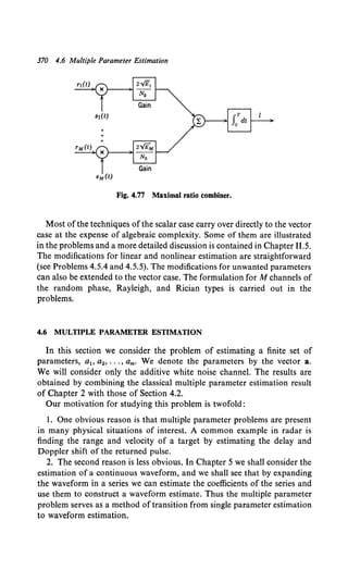
388. 372 4.6 Multiple Parameter Estimation
Assuming that the noise is white and that (445) holds, it follows in the
same manner as the scalar case that the MAP estimates are solutions to the
following set of M simultaneous equations:
0 = {2. rTf 8s(t, A) [r(t) - s(t, A)] dt + 8ln Pa,(A;)}I '
No JTt 8A; 8A; A=ilmap
(i = 1, 2, ... , M). (446)
If the a1 are Gaussian with zero-mean and variances aa1
2 , the equations
reduce to a simple form:
A 2aa,2
iT' os(t, A) I
a, = ~ ay- [r(t) - s(t, A)] dt . ,
0 Tt I A=amap
(i = 1, 2, ... , M).
(447)
This set of simultaneous equations imposes a set of necessary conditions
on the MAP estimates. (We assume that the maximum is interior to the
allowed region of A and that the indicated derivatives exist at the
maximum.)
The second result of interest is the bound matrix. From Section 2.4.3
we know that the first step is to find the information matrix. From
Equation 2.289
JT = JD + Jp,
(82 ln A(A))
Jv,, = -E 8A1 8A1 '
and for a Gaussian a priori density
Jp = Aa-1,
(448)
(449)
(450)
where Aa is the covariance matrix. The term in (449) is analogous to (104)
in Section 4.2. Thus it follows easily that (449) reduces to,
J = 2_ E [iT' 8s(t, A) 8s{t, A) d ] .
Dll lT a 8A 8A. t
lYQ Tt t 1
(451)
We recall that this is a bound with respect to the correlation matrix R,
in the sense that
(452)
is nonnegative definite. If the a posteriori density is Gaussian, R, - 1 = JT.
A similar result is obtained for unbiased estimates of nonrandom
variables by letting Jp = 0. The conditions for the existence of an efficient
estimate carry over directly. Equality will hold for the ith parameter if and
only if
K rTf 8s(t A)
d1[r(t)] - A1 = 1~ k;(A) JT; [r(t) - s(t, A)] at-dt. (453)
To illustrate the application of this result we consider a simple example.

389. Additive White Gaussian Noise Channel 373
Example. Suppose we simultaneously amplitude- and frequency-modulate a sinusoid
with two independent Gaussian parameters a, N(O, a.), and b, N(O, a0). Then
r(t) = s(t, A, B) + w(t) = e:)y, B sin (wet + {JAt) + w(t);
The likelihood function is
} JT/2 [ (2£)Y, ]
ln A[r(t)IA, B] = No -T/2 2r(t) - T B sin (wet + fJAt)
(2£)Yz
X T B sin (wet + flAt) dt.
Then
os(t A B) (2£)Yz
eA. = T B {Jt cos (wet + fJAt)
and
os(t, A, B) (2£)Yz . ( {JA )
i!B = T sm wet + t .
Because the variables are independent, JP is diagonal.
The elements of JT are
2 JT/2 2£ 1
Ju = N E... -T B 2fl2t 2 cos• (wet + flAt) dt + ----,
o -m ~
T 2 2E 1
~ ao• - - fJ" + 2'
- 12 No aa
2 JT/2 2£ . 2 1 2£ 1
J22 = ...,-Ea,o -T sm (wet+ flAt)+ 2 ~ u + 2'
,.o -m ~ ,.o ~
and
= ~0 E•.•[f~2 2
: Bflt sin (wet+ flAt) cos (wet +flAt) dt] ~ 0.
Thus the J matrix is diagonal. This means that
E[(d - a)•] ;:::: (_!_ + ao2T• 2£ f12)- 1
a,; 12 No
and
(455)
(456)
(457)
(458)
(459)
(460)
(461)
(462)
Thus we observe that the bounds on the estimates of a and b are uncorrelated. We
can show that for large E/No the actual variances approach these bounds.
We can interpret this result in the following way. If, each time the experiment was
conducted, the receiver were given the value of b, the performance in estimating a
would not be improved over the case in which the receiver was required to estimate b
(assuming large E/N0}.
We observe that there are two ways in which J 12 can be zero. If
JT12 os(t, A, B) os(t, A, B) d = 0
i!A i!B t
-T/2
(463)
before the expectation is taken, it means that for any value of A or B the partial
derivatives are orthogonal. This is required for ML estimates to be uncoupled.

390. 374 4.7 Summary and Omissions
Even if the left side of (463) were not zero, however, the value after taking the
expectation might be zero, which gives uncoupled MAP estimates.
Several interesting examples of multiple parameter estimation are
included in the problems.
4.6.2 Extensions
The results can be modified in a straightforward manner to include
other cases of interest.
l. Nonrandom variables, ML estimation.
2. Additive colored noise.
3. Random phase channels.
4. Rayleigh and Rician channels.
5. Multiple received signals.
Some of these cases are considered in the problems. One that will be
used in the sequel is the additive colored noise case, discussed in Problem
4.6.7. The results are obtained by an obvious modification of (447) which
is suggested by (226).
a,= ua,2 (T' os~~ A)l . [r9(z) - g(z)) dz, i = 1, 2, ... , M, (464)
JT, I A=amap
where
r9(z) - g(z) ?;:. IT' Qn(z, u)[r(u) - s(u, imap)] du, T1 ~ z ~ T1• (465)
JT,
4.7 SUMMARY AND OMISSIONS
4.7.1 Summary
In this chapter we have covered a wide range of problems. The central
theme that related them was an additive Gaussian noise component. Using
this theme as a starting point, we examined different types of problems and
studied their solutions and the implications of these solutions. It turned
out that the formal solution was the easiest part of the problem and that
investigating the implications consumed most of our efforts. It is worth-
while to summarize some of the more general results.
The simplest detection problem was binary detection in the presence of
white Gaussian noise. The optimum receiver could be realized as a
matched filter or a correlation receiver. The performance depended only
on the normalized distance between the two signal points in the decision

391. Summary 375
space. This distance was characterized by the signal energies, their correla-
tion coefficient, and the spectral height of the additive noise. For equal
energy signals, a correlation coefficient of -1 was optimum. In all cases
the signal shape was unimportant. The performance was insensitive to the
detailed assumptions of the model.
The solution for the M signal problem followed easily. The receiver
structure consisted of at most M - I matched filters or correlators.
Except for a few special cases, performance calculations for arbitrary cost
assignments and a priori probabilities were unwieldy. Therefore we devoted
our attention to minimum probability of error decisions. For arbitrary
signal sets the calculation of the probability of error was still tedious. For
orthogonal and nonorthogonal equally-correlated signals simple expres-
sions could be found and evaluated numerically. Simple bounds on the
error probability were derived that were useful for certain ranges of
parameter values. The question of the optimum signal set was discussed
briefly in the text and in more detail in the problems. We found that for
large M, orthogonal signals were essentially optimum.
The simple detection problem was then generalized by allowing a non-
white additive Gaussian noise component. This generalization also in-
cluded known linear channels. The formal extension by means of the
whitening approach or a suitable set of observable coordinates was easy.
As we examined the result, some issues developed that we had not en-
countered before. By including a nonzero white noise component we
guaranteed that the matched filter would have a square-integrable impulse
response and that perfect (or singular) detection would be impossible. The
resulting test was stable, but its sensitivity depended on the white noise
level. In the presence of a white noise component the performance could
always be improved by extending the observation interval. In radar this
was easy because of the relatively long time between successive pulses.
Next we studied the effect of removing the white noise component. We saw
that unless we put additional" smoothness" restrictions on the signal shape
our mathematical model could lead us to singular and/or unstable tests.
The next degree of generalization was to allow for uncertainties in the
signal even in the absence of noise. For the case in which these uncertainties
could be parameterized by random variables with known densities, the
desired procedure was clear. We considered in detail the random phase
case and the random amplitude and phase case. In the random phase
problem, we introduced the idea of a simple estimation system that
measured the phase angle and used the measurement in the detector. This
gave us a method of transition from the known signal case to situations,
such as the radar problem, in which the phase is uniformly distributed.
For binary signals we found that the optimum signal set depended on the

392. 376 4.7 Summary and Omissions
quality of the phase measurement. As we expected, the optimum correla-
tion coefficient ranged from p = -1 for perfect measurement to p = 0
for the uniform density.
The random amplitude and phase case enabled us to model a number of
communication links that exhibited Rayleigh and Rician fading. Here we
examined no-measurement receivers and perfect measurement receivers.
We found that perfect measurement offered a 6-db improvement. However,
even with perfect measurement, the channel fading caused the error prob-
ability to decrease linearly with Er/N0 instead of exponentially as in a
nonfading channel.
We next considered the problem of multiple channel systems. The
vector Karhunen-Loeve expansion enabled us to derive the likelihood
ratio test easily. Except for a simple example, we postponed our discussion
of vector systems to later chapters.
The basic ideas in the estimation problem were similar, and the entire
formulation up through the likelihood function was identical. For linear
estimation, the resulting receiver structures were identical to those obtained
in the simple binary problem. The mean-square estimation error in white
noise depended only on E/N0 •
The nonlinear estimation problem gave rise to a number of issues. The
first difficulty was that a sufficient statistic did not exist, which meant that
the mapping from the observation space to the estimation space depended
on the parameter we were trying to estimate. In some cases this could be
accommodated easily. In others approximate techniques were necessary.
The resulting function in the estimation space had a number of local
maxima and we had to choose the absolute maximum. Given that we were
near the correct maximum, the mean-square error could be computed
easily. The error could be reduced significantly over the linear estimation
error by choosing a suitable signaling scheme. If we tried to reduce the
error too far, however, a new phenomenon developed, which we termed
threshold. In the cascade approximation to the optimum estimator the
physical mechanism for the occurrence of a threshold was clear. The first
stage chose the wrong interval in which to make its local estimate. In the
continuous realization (such as range estimation) the occurrence was clear
but a quantitative description was more difficult. Because the actual
threshold level will depend on the signal structure, the quantitative results
for the particular example discussed are less important than the realization
that whenever we obtain an error decrease without an increase in signal
energy or a decrease in noise level a threshold effect will occur at some
signal-to-noise level.
The final problem of interest was multiple-parameter estimation. This
served both to complete our discussion and as a starting point for the

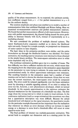
393. Topics Omitted 377
problem of waveform estimation. Here the useful results were relations
that showed how estimation errors were coupled by the signal structure
and the a priori densities.
In addition to summarizing what we have covered, it is equally important
to point out some related issues that we have not.
4.7.2 TOPICS OMITTED
Digital Communications. We have done a great deal of the groundwork
necessary for the study of modern digital systems. Except for a few cases,
however, we have considered only single-digit transmission. (This is
frequently referred to as the one-shot problem in the literature.) From the
simple example in Section 4.2 it is clear that performance can be improved
by transmitting and detecting blocks of digits. The study of efficient
methods is one ofthe central problems ofcoding theory. Suitable references
are given in [66] and [18]. This comment does not imply that all digital
communication systems should employ coding, but it does imply that
coding should always be considered as one of the possible alternatives in
the over-all system design.
Non-Gaussian Interference. It is clear that in many applications the
prime source of interference is non-Gaussian. Simple examples are man-
made interference at lower frequencies, impulse noise, and galactic, solar,
and atmospheric noise.
Our reason for the omission of non-Gaussian interferences is not because
of a lack of interest in or appreciation of their importance. Neither is it
because of our inability to solve a particular non-Gaussian problem. It is
probable that if we can model or measure the pertinent statistics adequately
a close-to-optimum receiver can be derived (e.g., [67], [68]). The reason is
that it is too difficult to derive useful but general results.
Our goal with respect to the non-Gaussian problem is modest. First, it
is to leave the user with an awareness that in any given situation we must
verify that the Gaussian model is either valid or an adequate approxima-
tion to obtain useful results. Second, if the Gaussian model does not hold,
we should be willing to try to solve the actual problem (even approximately)
and not to retain the Gaussian solution because of its neatness.
In this chapter we have developed solutions for the problems ofdetection
and finite parameter estimation. We now turn to waveform estimation.
4.8 PROBLEMS
The problems are divided according to sections in the text. Unless
otherwise stated, all problems use the model from the corresponding

394. 378 4.8 Problems
section of the text; for example, the received signals are corrupted by
additive zero-mean Gaussian noise which is independent of the hypotheses.
Section P4.2 Additive White Gaussian Noise
BINARY DETECTION
Problem 4.2.1. Derive an expression for the probability of detection Po, in terms of d
and PF, for the known signal in the additive white Gaussian noise detection problem.
[see (37) and (38)].
Problem 4.2.2. In a binary FSK system one of two sinusoids of different frequencies
is transmitted; for example,
sl(t) = f(t) cos 2rrfct,
s2(t) = /(t) cos 2rr(fc + tlf)t,
OStST,
OStST,
where lc » 1/T and tJ.f. The correlation coefficient is
J:f2(t)cos(2rr6./t)dt
p = T •
fo f"(t) dt
The transmitted signal is corrupted by additive white Gaussian noise (N0/2).
1. Evaluate p for a rectangular pulse; that is,
f(t) = e:r.
= 0,
Sketch the result as a function of tJ.fT.
OStST,
elsewhere.
2. Assume that we require Pr (f) = 0.01. What value of E/No is necessary to achieve
this iftJ.f = oo? Plot the increase in E/No over this asymptotic value that is necessary
to achieve the same Pr (f) as a function of tJ.fT.
Problem 4.2.3. The risk involved in an experiment is
:R. = CFPFPo + CMPMP1.
The applicable ROC is Fig. 2.9. You are given (a) CM = 2; (b) CF = 1; (c) P1 may
vary between 0 and 1. Sketch the line on the ROC that will minimize your maximum
possible risk (i.e., assume P1 is chosen to make :R. as large as possible. Your line
should be a locus of the thresholds that will cause the maximum to be as small as
possible).
Problem 4.2.4. Consider the linear feedback system shown below
w(t)
+
r(t)
x(t)
+
Fig. P4.1

395. Additive White Gaussian Noise 379
The function x(t) is a known deterministic function that is zero for t < 0. Under
H, A, = A,. Under Ha, A, = Ao. The noise w(t) is a sample function from a white
Gaussian process of spectral height N0/2. We observe r(t) over the interval (0, T).
All initial conditions in the feedback system are zero.
1. Find the likelihood ratio test.
2. Find an expression for Pn and PF for the special case in which x(t) = S(t)
(an impulse) and T = CXJ.
Problem 4.2.5. Three commonly used methods for transmitting binary signals over an
additive Gaussian noise channel are on-off keying (ASK), frequency-shift keying
(FSK), and phase-shift keying (PSK):
Ho:r(t) = sa(t) + w(t),
H1:r(t) = s1(t) + w(t),
OStST,
ostsT,
where w(t) is a sample function from a white Gaussian process of spectral height
No/2. The signals for the three cases are as follows:
ASK
I FSK
I PSK
so(I)
I 0
I V2E/Tsin w1t
I V2E/Tsin wot
s1(t)
I v'2E/T sin w1t
I V2E/Tsin w0t
I V2E/Tsin (w0t + ,.)
where w0 - w1 = 2,.n/T for some nonzero integer n and wo = 2,.mT for some
nonzero integer m.
l. Draw appropriate signal spaces for the three techniques.
2. Find d2 and the resulting probability of error for the three schemes (assume that
the two hypotheses are equally likely).
3. Comment on the relative efficiency of the three schemes (a) with regard to
utilization of transmitter energy, (b) with regard to ease of implementation.
4. Give an example in which the model of this problem does not accurately describe
the actual physical situation.
Problem 4.2.6. Suboptimum Receivers. In this problem we investigate the degradation
in performance that results from using a filter other than the optimum receiver
filter. A reasonable performance comparison is the increase in transmitted energy
required to overcome the decrease in d2 that results from the mismatching. We would
hope that for many practical cases the equipment simplification that results from
using other than the matched filter is well worth the required increase in transmitted
energy. The system of interest is shown in Fig. P4.2, in which
LTs2(t) dt = l and E[w(t) w(r)] = ~0 3(t - r).
Ht:-./Es(t) j
Ho:O
OStST
w(t)
Sub-optimum receiver
Fig. P4.2

396. 380 4.8 Problems
The received waveform is
We know that
and
Suppose that
H1:r(t) = v£ s(t) + w(t),
Ho:r(t) = w(t),
{
s(T- 1),
hopt(l) =
0,
{
( 1)''
s(t) = T '
0,
-co < t < co,
-co < t < co.
O:St:ST,
elsewhere,
-co < t < co,
O:St:ST,
elsewhere.
1. Choose the parameter a to maximize the output signal-to-noise ratio d2 •
2. Compute the resulting d2 and compare with d:pt· How many decibels must the
transmitter energy be increased to obtain the same performance?
M-ARY SIGNALS
Problem 4.2.7. Gram-Schmidt. In this problem we go through the details of the
geometric representation of a set of M waveforms in terms of N(N :S M) orthogonal
signals.
Consider the M signals s1{t), ... , sM(t) which are either linearly independent or
linearly dependent. If they are linearly dependent, we can write (by definition)
M
L a1s1(t) = 0.
1=1
I. Show that if M signals are linearly dependent, then sM(t) can be expressed in
termsofs1(t):i= 1, ...,M-l.
2. Continue this procedure until you obtain N-linearly independent signals and
M-N signals expressed in terms of them. N is called the dimension of the signal set.
3. Carry out the details of the Gram-Schmidt procedure described on p. 258.
Problem 4.2.8. Translation/Simplex Signals [18]. For maximum a posteriori reception
the probability of error is not affected by a linear translation of the signals in the
decision space; for example, the two decision spaces in Figs. P4.3a and P4.3b have
the same Pr (E). Clearly, the sets do not require the same energy. Denote the average
energy in a signal set as
M M f.T
E fl 1~ Pr (H1) lsd2 = 1~1Pr (H,)E, 0
s,2(t) dt.
1. Find the linear translation that minimizes the average energy of the translated
signal set; that is, minimize
M
E ~ L Pr (H1)Is1 -ml2 •
1=1

397. Additive White Gaussian Noise 381
!pz
81 82 81 B2
X X X
fo'l fo'l
84 sa
'"
X X X
(a) (b)
Fig. P4.3
2. Explain the geometric meaning of the result in part 1.
3. Apply the result in part 1 to the case of M orthogonal equal-energy signals
representing equally likely hypotheses. The resulting signals are called Simplex
signals. Sketch the signal vectors for M = 2, 3, 4.
4. What is the energy required to transmit each signal in the Simplex set?
5. Discuss the energy reduction obtained in going from the orthogonal set to the
Simplex set while keeping the same Pr (£).
Problem 1.2.9. Eqully correlated signals. Consider M equally correlated signals
1. Prove
1
-M-l:Sp:Sl.
j = j,
i,.j.
2. Verify that the left inequality is given by a Simplex set.
3. Prove that an equally-correlated set with energy E has the same Pr (£) as an
orthogonal set with energy Eorth = E(l - p).
4. Express the Pr (E) of the Simplex set in terms of the Pr (£)for the orthogonal set
andM.
Problem 1.2.10. M Signals, Arbitrary Correlation. Consider an M-ary system used to
transmit equally likely messages. The signals have equal energy and may be correlated:
P•1 = LTs,(t) s1(t) dt, i,j= 1,2, ...,M.
The channel adds white Gaussian noise with spectral height No/2. Thus
r(t) = v'£ s1(t) + w(t), i = l, ...,M.
1. Draw a block diagram of an optimum receiver containing M matched filters.
What is the minimum number of matched filters that can be used?
2. Let p be the signal correlation matrix. The ij element is p,1• If pis nonsingular,
what is the dimension of the signal space?
3. Find an expression for Pr (£1H,), the probability of error, assuming H, is true.
Assume that p is nonsingular.
4. Find an expression for Pr (E).
5. Is this error expression valid for Simplex signals? (Is p singular?)

398. 382 4.8 Problems
Problem 4.2.11 (contiiUUition). Error Probability [69]. In this problem we derive an
alternate expression for the Pr (e) for the system in Problem 4.2.10. The desired
expression is
1- Pr (£) = itexp (-!)J_:exp [(~* x]
[ d I" I" exp (-!i"p-1y) ]
x dx -.. • . . -.. (2,.)MiliiPI* dy dx. (P.l)
Develop the following steps:
1. Rewrite the receiver in terms of M orthonormal functions •Mt). Define
M
s,(t) = zs,k 4>k(t), i=1,2, ... ,M,
k•l
..
r(t) = zr,. ."(t).
lc•l
Verify that the optimum receiver forms the statistics
and chooses the greatest.
2. Assume that sm(t) is transmitted. Show
Pr (ilm) ~ Pr (R in Zm)
= Pr ( f Sm"R" =max i ss~cR~c)·
lc=l I k=l
3. Verify that
P (-) 1 ( E) ~ J'" J'" exp [-(1/No) ~~=1 R~c2]
r£ =-exp -- L.. •••
M No m•l -., -., (trNo)Mill
x exp ( ..~ max~ R~css~c)· (P.2)
Ho I k=l
4. Define
and observe that (P.2) can be viewed as the expectation of/(R) over a set ofstatistically
independent zero-mean Gaussian variables, R~c, with variance N0 /2. To evaluate this
expectation, define
j = 1, 2, ... , M,
and
Find p.(z). Define

399. Additive White Gaussian Noise 383
Findpx(x).
5. Using the results in (4), we have
1 - Pr (•) =~exp (-!Jr..exp [ (~)* x]p.,(X) dX.
Use p.,(X) from (4) to obtain the desired result.
Problem 4.2.11 (t:olfti,ation).
1. Using the expression in (P.1) of Problem 4.2.11, show that 8 Pr (•)/8p12 > 0.
Does your derivation still hold if 1 -+ i and 2 -+ j?
2. Use the results of part 1 and Problem 4.2.9 to develop an intuitive argument
that the Simplex set is locally optimum.
Comment. The proof of local optimality is contained in [70]. The proof of global
optimality is contained in [71].
Problem 4.2.13. Consider the system in Problem 4.2.10. Define
Pmaz = ~~~ Pil•
1. Prove that Pr (•) on any signal set is less than the Pr (•) for a set of equally
correlated signals with correlation equal to Pmax·
2. Express this in terms of the error probability for a set of orthogonal signals.
3. Show that the Pr (•) is upper bounded by
Pr (•) S(M- 1) {erfc• ([!0 (1 - Pmax>r'}
Problem 4.2.U (72]. Consider the system in Problem 4.2.10. Define
d,:distance between the ith message point and the nearest neighbor.
Observe
dmln = min d,.
I
Prove
erfc.(J) S Pr(•) S (M-l)erfc.(dmtn)
Note that this result extends to signals with unequal energies in an obvious manner.
Problem 4.2.15. In (68) of the text we used the limit
lim In erf• [>' + (2PT~ogm Mrl.
M~., 1/(M- 1)
Use !'Hospital's rule to verify the limits asserted in (69) and (70).
Problem 4.1.16. The error probability in (66) is the probability of error in deciding
which signal was sent. Each signal corresponds to a sequence of digits; for example,
if M= 8,
000 --+- so(t)
001-+sl(t)
010-+ s2(t)
Oll-+s3(t)
100-+s.(t)
101-+sa(t)
110-+ s8 (t)
lll-+s7(t).

400. 384 4.8 Problems
Therefore an error in the signal decision does not necessarily mean that all digits
will be in error. Frequently the digit (or bit) error probability [Prs (€)] is the error of
interest.
I. Verify that if an error is made any of the other M - I signals are equally likely
to be chosen.
2. Verify that the expected number of bits in error, given a signal error is made, is
(log2 M)M
2(M- 1).
3. Verify that the bit error probability is
M
Prs (€) = 2(M _ 1) Pr (£).
4. Sketch the behavior of the bit error probability for M = 2, 4, and 8 (use Fig.
4.25).
Problem 4.1.17. Bi-orthogonal Signals. Prove that for a set of M bi-orthogona1 signals
with energy E and equally likely hypotheses the Pr (€) is
Pr (€) = 1 - .;-exp -- (x- V£)2 .;-exp -- dy dx.
f.oo 1 [ 1 - ][J" 1 ( y2) ]M/2-1
0 v wN0 No -" v wN0 No
Verify that this Pr (€) approaches the error probability for orthogonal signals for
large M and d2• What is the advantage of the hi-orthogonal set?
Problem 4.1.18. Consider the following digital communication system. There are four
equally probable hypotheses. The signals transmitted under the hypotheses are
OStST,
OStST,
OStST,
OStST.
2wn
Wc=T
The signal is corrupted by additive Gaussian white noise w(t), (No/2).
1. Draw a block diagram of the minimum probability of error receiver and the
decision space and compute the resulting probability of error.
2. How does the probability of error behave for large A"/No?
Problem 4.1.19. M-ary ASK [72]. An ASK system is used to transmit equally likely
messages
s,(t) = vE; </>(t), i = 1, 2, ..., M,
where
vE; = <;- I)~. s:'/>2( t) dt = 1.

401. Additive White Gaussian Noise 385
The received signal under the ith hypothesis is
r(t) = s,(t) + w(t),
where w(t) is a white noise with spectral height No/2.
1. Draw a block diagram of the optimum receiver.
2. Draw the decision space and compute the Pr (£).
3. What is the average transmitted energy?
~1 n~ •2 (n - 1) n(2n - 1)
note. L... J = 6 ·
l=l
i =I, 2, ..., M,
4. What translation of the signal set in the decision space would maintain the
Pr (£)while minimizing the average transmitted energy?
Problem 4.2.20 (continuation). Use the sequence transmission model on pp. 264-265
with the ASK system in part 4 of Problem 4.2.19. Consider specifically the case in
which M = 4. How should the digit sequence be mapped into signals to minimize
the bit error probability? Compute the signal error probability and the bit error
probability.
Problem 4.2.21. M-ary PSK [72]. A communication system transmitter sends one of
M messages over an additive white Gaussian noise channel (spectral height No/2)
using the signals
{(2£)Y. ( n 2"i)
s,(t) = T cos 21T T t + M ,
0, elsewhere, i = 0, 1, 2, ..., M- 1,
where n is an integer. The messages are equally likely. This type of system is called
an M-ary phase-shift-keyed (PSK) system.
1. Draw a block diagram of the optimum receiver. Use the minimum number of
filters.
2. Draw the decision-space and decision lines for various M.
3. Prove
where
((2£)% 7T)
a = erfc* No sin M ·
Problem 4.2.22 (continuation). Optimum PSK [73]. The basic system is shown in
Fig. 4.24. The possible signaling strategies are the following:
1. Use a binary PSK set with the energy in each signal equal to PT.
2. Use an M-ary PSK set with the energy in each signal equal to PT logz M.
Discuss how you would choose M to minimize the digit error probability. Compare
hi-phase and four phase PSK on this basis.
Problem 4.2.23 (continuation). In the context of an M-ary PSK system discuss qualita-
tively the effect of an incorrect phase reference. In other words, the nominal signal

402. 386 4.8 Problems
set is given in Problem 4.2.22 and the receiver is designed on that basis. The actual
signal set, however, is
{(
2£)Y' (2..n 2..; )
- cos -t+-+8·
s,(t) = T T M
0,
O~t~T.
elsewhere,
i = 1, 2, ... , M,
n is an integer,
where 8 is a random phase angle. How does the importance of a phase error change
as M increases?
EsTIMATION
Problem 4.2.24. Bhattacharyya Bound. Let
r(t) = s(t, A) + w(t), O~t~T.
where s(t, A) is differentiable k times with respect to A. The noise has spectral height
No/2.
1. Extend the Bhattacharyya bound technique developed in Problem 2.4.23 to the
waveform for the n = 2 case. Assume that A is nonrandom variable.
2. Repeat for the case in which A is a Gaussian random variable; N(O, ua).
3. Extend the results in parts I and 2 to the case in which n = 3.
Problem 4.2.25. Consider the problem in Example 1 on p. 276. In addition to the
unknown time of arrival, the pulse has an unknown amplitude. Thus
r(t) = b s(t - a) + w(t), -T ~ t ~ T,
where a is a uniformly distributed random variable (see Fig. 4.29b) and b is Gaussian,
N(O, u.).
Draw a block diagram of a receiver to generate the joint MAP estimates, dmap
and hmap•
Problem 4.2.26. The known signal s(t), 0 ~ t ~ T, is transmitted over a channel
with unknown nonnegative gain A and additive Gaussian noise n(t):
LTs2 (t) dt = E,
No
K.(t• ..) = 2 au - ..).
1. What is the maximum likelihood estimate of A?
2. What is the bias in the estimate?
3. Is the estimate asymptotically unbiased?
Problem 4.2.27. Consider the stationary Poisson random process x(t). A typical
sample function is shown in Fig. P4.4.
/Event times
--~0~~~-x--~~-----~--*~~T----~
Fig. P4.4

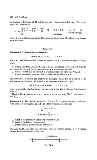
403. Nonwhite Additive Gaussian Noise 387
The probability of n events in any interval ,. is
(h)"
Pr (n, ,.) = - 1
- e-k•.
n.
The parameter k of the process is an unknown nonrandom variable which we want
to estimate. We observe x(t) over an interval (0, n.
1. Is it necessary to record the event times or is it adequate to count the number
of events that occur in the interval? Prove that n•, the number of events that occur
in the interval (0, T) is a sufficient statistic.
2. Find the Cramer-Rao inequality for any unbiased estimate of k.
3. Find the maximum-likelihood estimate of k. Call this estimate !c.
4. Prove that k is unbiased.
5. Find
Var (k- k).
6. Is the maximum-likelihood estimate efficient?
Problem 4.2.28. When a signal is transmitted through a particular medium, the
amplitude of the output is inversely proportional to the murkiness of the medium.
Before observation the output of the medium is corrupted by additive, white Gaussian
noise. (Spectral height N0 /2, double-sided.) Thus
1
r(t) = M f(t) + w(t), 0:5t:5T,
where/(t) is a known signal and
I:J2(t) dt =E.
We want to design an optimum Murky-Meter.
1. Assume that M is a nonrandom variable. Derive the block diagram of a system
whose output is the maximum-likelihood estimate of M (denoted by mm1).
2. Now assume that M is a Gaussian random variable with zero mean and variance
oM2 . Find the equation that specifies the maximum a posteriori estimate of M (denoted
by mmap).
3. Show that
as
Section 4.3 Nonwhite Additive Gaussian Noise
MATHEMATICAL PRELIMINARIES
Problem 4.3.1. Reversibility. Prove that hw(t, u) [defined in (157)] is a reversible
operation by demonstrating an hw -'(t, u) such that
J
T1
hw(t, u) hw -l(u, z) du = a(t - z).
Tl
What restrictions on the noise are needed?

404. 388 4.8 Problems
Problem 4.3.2. We saw in (163) that the integral equation
No IT'
2 ho(Z, v) + h0(V, x) Kc(X, z) dx = Kc(Z, v),
T,
1i S z, v s T1,
specifies the inverse kernel
2
Q.(t, T) = No (8(t - T) - h0(t, T)].
Show that an equivalent equation is
No JT'
2 ho(z, v) + T, ho(Z, v) Kc(X, v) dx = Kc(z, v),
Problem 4.3.3 [74] We saw in Problem 4.3.2 that the inverse kernel Q.(t, T) can be
obtained from the solution to an integral equation:
No JT'
2 ho(t, T) + T, ho(t, u) Kc(U, T) du = Kc(t, T),
where
2
Q.(t, T) = No (8(t - T) - h0 (t, T)].
Suppose we let T1, the end point of the interval, be a variable. We indicate this by
writing h.(t, T: T1) instead of h.(t, T):
Now differentiate this equation with respect to T1 and show that
oh.(t,T:T,) h( T T)h(T T)
oTt = - o t, 1: I o /o T: I •
Hint.
has no solution for .. < 0.
Problem 4.3.4. RealiT.able Whitening Filters [91] In the text, two equivalent realiza-
tions of the optimum receiver for the colored noise problem were given in Figs. 4.38a
and b. We also saw that Q.(t, u) was an unrealizable filter specified by (162) and (163).
Furthermore, we found one solution for h.,(t, T), the whitening filter, in terms of
eigenfunctions that was an unrealizable filter. We want to investigate the possibility of
finding a realizable whitening filter. Recall that we were able to do so in the simple
example on p. 311.
1. Write down the log-likelihood ratio in terms of ho(t, T) = h.(t, T:T1) (see
Problem 4.3.3).
2. Write
fT' [fT' - ][JT' ] JT' oL(t)
In A(r(t)) = T, dt JT, h.,..(t, u) v'E s(u) du T, h,.,(t, z) r (z) dz £ L(T1
)= T, -a1 dt.

405. Nonwhite Additive Gaussian Noise 389
The additional subscript r denotes realizable.
3. Use the result from Problem 4.3.3 that
8h.(u, v:t) h ( )h ( )
at = - • t, u:t • t, v:t
to show that
h.,,(t, u) = (~J%[1l(t - u) - h.(t, u: t)).
Observe that h.(t, u: t) is a realizable filter.
4. Write down the integral equation satisfied by h.(t, T:t). In Chapter 6 we discuss
techniques for solving this equation.
Problem 4.3.5. M-ary Signals, Colored Noise. Let the received signal on the ith
hypothesis be
r(t) = v£, s1(t) + n.(t) + w(t), T1 :s; t :s; T1 :H., i = 1, 2, ... , M,
where w(t) is zero-mean white Gaussian noise with spectral height No/2 and n.(t) is
independent zero-mean colored noise with covariance function K.(t, u). The signals
s,(t) are normalized over (0, T) and are zero outside that interval. Assume that the
hypotheses are equally likely and that the criterion is minimum Pr (€), Draw a block
diagram of the optimum receiver.
EsTIMATION
Problem 4.3.6. Consider the following estimation problem:
3
r(t) = A s(t) + L b,s,(t) + w(t), 0 :s; t :s; T,
f=l
where A is a nonrandom variable, b, are independent, zero-mean, Gaussian random
variables [E(b12) = a12], w(t) is white noise (N0 /2), s(t) = ~}= 1 c,s,(t),
f~ s,(t) sJ(t) dt = ll1~o and f~ = s2(t) dt = 1.
I. Draw a block diagram of the maximum-likelihood estimator of A, dml•
2. Choose c1, c2, c3 to minimize the variance of the estimate.
INTEGRAL EQUATION SOLUTIONS
Problem 4.3.7. In this problem we solve a simple Fredholm equation of the second
kind,
where
• /- N, (Tt
v E s(t) = 2°g(t) + JT, K.(t, u) g(u) du,
K.(t, u) = ac2 exp [-kit- u!J.
1
s(t) = VT
T. = 0,
T1 = T.
0 :s; t :s; T,
1. Find g(t).
2. Evaluate the performance index d2•
T, :s; t :s; T1,

406. 390 4.8 Problems
Problem 4.3.8 (contiiUlation). Solve Problem 4.3.7 for the case in which 7j = - oo and
T1 = oo. Compare the value of d2 that you obtain with the value obtained in that
problem.
Problem 4.3.9. Solve the Fredholm equation of the first kind,
f K(t, u) g(u) = s(t), O:St:ST,
for the triangular kernel
K( '" _ {1 - It - ul for It - ul < 1,
t, u, - 0, elsewhere.
Assume that s(t) is twice differentiable and that T < l.
Now apply this result to the problem of detecting a known signal s(t), 0 S t S T,
which is observed in additive Gaussian noise with covariance
K (t u) = {1 - It - ul for It - ul S 1,
• ' 0, elsewhere.
1. What is the optimum receiver ? Note that we cannot physically generate impulses
so that correlation with g(t) is not a satisfactory answer.
2. Calculate d2•
What is a necessary and sufficient condition for singular detection in this problem
if s(t) is bounded?
Problem 4.3.10.
l. Evaluate d2 for the example given on p. 318.
2. Provided tliat s(t) is bounded and has finite energy, what is a necessary and
sufficient condition on s(t) for a nonsingular test?
Problem 4.3.11 (contiiUlation). The optimum receiver for Problem 4.3.10 includes a
matched filter plus a sampler. Find d2 for the suboptimum receiver that has the
matched filter but not the sampler.
Problem 4.3.12. The opposition is using a binary communication system to transmit
data. The two signals used are the following:
) • 2 211"
s1(t = sm T t,
s0(t) = -sin2 ~ t,
The received signal is either
H 1 :r(t) = s1 (t) + n(t),
H0 :r(t) = s0(t) + n(t),
O:St:ST,
O:St:ST.
O:St:ST,
O:St:ST,
where n(t) is a sample function from a zero-mean Gaussian random process with
covariance function
Kn(T) = e·al<l.
Assume that he knows a and builds a min Pr (E) receiver. Choose a to minimize his
performance.

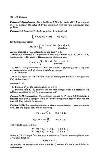
407. Nonwhite Additive Gaussian Noise 391
SENSITIVITY AND SINGULARITY
Problem 4.3.13. Singrdarity [2]. Consider the simple binary detection problem shown
in Fig. P4.S. On H1 the transmitted signal is a finite energy signal x(t). On Ho there
is no transmitted signal. The additive noise w(t) is a sample function from a white
process 1v2 /cps). The received waveform r(t) is passed through a filter whose transfer
function is H(jw). The output y(t), 0 ::s; t ::s; Tis the signal available for processing.
Let .k and 4>k(t) be the eigenvalues and eigenfunctions, respectively, of n(t), 0 ::s; t ::s; T.
To have singular detection, we require
., s 2
L...!!.. =oo.
k~l ,k
We want to prove that this cannot happen in this case.
1. From
sk = J:Mt) s(t) dt
show that
sk = r.. X(/) H(j2w/) 4>t(f) d/,
where
X(/) = J:., x(t)e- 12ntt dt
and
4>k(/) = f"' 4>k(t)e-12nft dt = fT 4>k(t)e-12nf1 dt.
- c Jo
2. Show that
ifm = k,
ifm ::F k.
3. Observe from part 2 that for some set of numbers ck
where
r.. U(f) H(j2wf) 4>:U>df = o.
4. Using (1), (2), and (3), show that
., s 2 J"'
k~l ;k ::s; - ... x2(t) dt,
hence that perfect detection is impossible in this situation.
w(t)
.--T-r-an_s_m-itt_e_r.,1 ~ !f----";o;o.tr;;)"l ;,
Ht:%(t) 0 ~ I
Ho: o s(t) + n(t)
y(t) = n(t)
Fig. P4.5
O::St::ST :H1
O::St::ST :Ho

408. 392 4.8 Problems
Problem 1.3.14. Consider the following system:
It is given that
H1 :r(l) = s1(1) + n(l),
H 0 :r(1) = n(l),
6 21T
n(l) = .~1 a. cos n T I,
OSIST,
osrsT.
where a. are zero-mean random variables. The signal energy is
J:s12 (t) dt = E.
Choose s1(t) and the corresponding receiver so that perfect decisions can' be made
with probability 1.
Problem 4.3.15. Because white noise is a mathematical fiction (it has infinite energy,
which is physically impossible), we sometimes talk about band-limited white noise;
that is,
{
No
s.(w) = T•
0, otherwise.
Now suppose that we wish to detect a strictly time-limited signal
s(t) = (¥)".
0,
OSIST,
otherwise.
Is this a good mathematical model for a physical problem? Justify your answer.
Problem 4.3.16. Sensitivity to White Noise Level. The received waveforms under the
two hypotheses are
r(t) = s(t) + n.(t) + w(t),
r(t) = nc(t) + w(t),
-oo <I< oo:H1o
-oo < t < oo:H0 •
The signal waveform s(t) and the colored noise spectrum S.(w) are known exactly.
The white noise level is
where No/2 is the nominal value and x is a small variation. Assume that the receiver
is designed on the basis of the nominal white noise level.
l. Find an expression for od~oxL=o = 8~';'L=o £! ~.
2. Assume that
and
s(t) = V2kP e-kt,
0,
I~ 0,
1 < 0
1kac2
s.c(w) = w• + k..
Evaluate~ as a function of A£! 4a."fkN0 •

409. Nonwhite Additive Gaussian Noise 393
Problem 4.3.17. Sensitivity to Noise Spectrum. Assume the same nominal model as in
Problem 4.;3.16.
1. Now let
and
where
Find
ka = k (1 + y)
a 4 2 = ac" (1 + z)
od~oy~~~% ~ fl. and od~oz~~~g ~ fl•.
2. Evaluate fly and fl. for the signal shape in Problem 4.3.16.
Problem 4.3.18. Sensitivity to Delay and Gain. The received waveforms under the two
hypotheses are
r(t) = v'F; s(t) + b1s(t - T} + w(t), - oo < t < oo :H1,
r(l) = brs(t- T) + w(l), -oo <I< oo:H0,
where br is N(O, ar) and w(t) is white with spectral height N0 /2. The signal is
s(l} =(~f.
= 0,
O:St:ST,
elsewhere.
1. Design the optimum receiver, assuming that Tis known.
2. Evaluate d2 as a function of Tand ar.
3. Now assume
Ta = T (1 + x).
Find an expression for d" of the nominal receiver as a function of x. Discuss the
implications of your results.
4. Now we want to study the effect of changing a1• Let
ara2 = ar" (1 + y)
and find an expression for d2 as a function of y.
LINEAR CHANNELS
Problem 4.3.19. Optimum Signals. Consider the system shown in Fig. 4.49a. Assume
that the channel is time-invariant with impulse response h(T) [or transfer function
H(f)]. Let
H(f) = l,
= 0,
1/1 < w,
otherwise.
The output observation interval is infinite. The signal input is s(l), 0 :S 1 :S T and is
normalized to have unity energy. The additive white Gaussian noise has spectral
height N0 /2.
1. Find the optimum receiver.
2. Choose s(t), 0 :S t :S T, to maximize d2•

410. 394 4.8 Problems
Problem 4.3.20. Repeat Problem 4.3.19 for the h(t, T) given below:
h(f, T) = a(t - T),
T T 3T
0 ~ T ~ 4' 2 ~ T ~ 4' - 00 < f < 00,
= 0, elsewhere.
Problem 4.3.21. The system of interest is shown in Fig. P4.6. Design an optimum
binary signaling system subject to the constraints:
I. J:s2 (t) dt = Ec.
2. s(t) = 0,
3. h(T) = e-k•,
= 0,
I< 0,
t < T.
T ~ 0,
T < 0.
Fig. P4.6
Section P.4.4 Signals with Unwanted Parameters
MATHEMATICAL PRELIMINARIES
w(t)(~o)
Formulas. Some of the problems in this section require the manipulation of Bessel
functions and Q functions. A few convenient formulas are listed below. Other
relations can be found in [75] and the appendices of [47] and [92]
I. Modified Bessel Functions
1 J.2n
ln(z) ~ 21T
0
exp ( ±jn8) exp (z cos 8) dB,
ln(Z) = L n(Z),
(tz)•
lv(z) ::::: r(v + 1)' v # -1, -2, ... ' z « 1,
e• [ 4v2 - 1]
I.(z) ::::: ---= 1 - - - •
v21rz 8z
z » 1,
1 dk
Zk dzk (z-v I.(z)) = z-•-kJv+k(z),
1 dk
?'dzk (z• I.(z)) = z•-kfv-k(z).
II. Marcum's Q-function [92]
Q(V2a, V2b) = f'exp (-a + x) l0(2Vax) dx,
Q(a, a) =t[l + lo(a2) exp (- a2)],
(F.l.l)
(F.1.2)
(F.l.J)
(F.l.4)
(F.l.S)
(F.l.6)
(F.2.1)
(F.2.2)

411. Signals with Unwanted Parameters 395
1 + Q(a, b) - Q(b, a)
b >a> 0,
_ a12
[t _ (J a1 2
, j a2 2
)]
- a12 + a22 Q al2 + a22 al2 + a22
Q(a, b) c:: erfc. (b - a), b » 1, b » b - a.
III. Rician variables [76]
(F.2.3)
(F.2.4)
(F.2..S)
Consider the two statistically independent Rician variables, x1 and x2 with prob-
ability densities,
The probability of interest is
P• = Pr [x2 > xd.
Define the constants
a?
a= '
a1 2 + a?
Then
.y- v'- c2
( a + b) .y-
P. = Q( a, b)- 1 + c 2 exp - -
2- lo( ab),
or
c2 • ;- • ;- 1 . ;- . ;-
P. = -
1- -
2 [1 - Q(v b, v a)] + -
1 - -
2 Q(v a, v b),
+ c + c
or
0 < ak < oo,
o < xk < oo,
k = 1, 2.
al
c =-·
a2
(F.3.1)
(F.3.2)
(F.3.3)
v'- v'- v'- v'- 1 c2
- 1 ( a + b) v'-
p• =t[l - Q( b, a) + Q( a, b)] - 2c2 + 1exp - -
2- lo( ab). (F.3.4)
Problem 4.4.1. Q-function Properties. Marcum's Q-function appears frequently in the
calculation of error probabilities:
Q(a, {l) = L'" x exp [-t(x2 + a2)] / 0(ax) dx.
Verify the following properties:
1. Q(a, 0) = 1,
2. Q(O, {l) = e-P212.
3. Q(a, {l) = e-<a2 +P2>
12 .~ (~)" I.(a{J), a < {3,
= 1 - e-<a2+p2JI2 i (~)" I.(a{l),
n=l a
fJ < a,

412. 396 4.8 Problems
4. Q(a, P) + Q(p, a) = 1 + (e-1" 2 +62 >12) / 0(ap).
5. Q(a, p) ~ 1 -a~ p(2~a)e-!«-6>212), a»P»l.
6. Q(a, p) ~ p ~ a (2!a)e-!6-al2
1•), P»a»l.
Problem 4.4.2. Let x be a Gaussian random variable N(m,, a,).
1. Prove that
M U. ) !!. E[ ( . ")] _ exp Uvm,"/(1 - 2jva,2)l.
,2 v _ exp +JVX - (1 _ 2jva,")"'
Hint.
M,•(jv) = [M,•(jv) M.•(jv)]Yz,
where y is an independent Gaussian random variable with identical statistics.
2. Let z be a complex number. Modify the derivation in part 1 to show that
3. Let
E[ (+ ")] _ exp [zm,2/(l - 2za,2)]
exp zx - (1 - 2za,•)v• '
2M
y• = L -x,•,
1=1
1
Re(z) < - ·
2a,2
where the x, are statistically independent Gaussian variables, N(m., a1).
Find M.•(jv) and E[exp (+zy2)]. What condition must be imposed on Re (z) in
order for the latter expectation to exist.
4. Consider the special case in which .1 = I and a,2 = a". Verify that the probability
density of y2 is
1 (y)M;' ( Y+Sa") [(YS)li]
p.•(Y) = 2a" Sa" exp - ~ IM-1 -;;> • y?: 0,
= 0, elsewhere,
where S = ~~~~ m12• (See Erdelyi [75], p. 197, eq. 18.)
Problem 4.4.3. Let Q(x) be a quadratic form ofcorrelated Gaussian random variables,
Q(x) !:= xTAx.
1. Show that the characteristic function of Q is
11 (')!!. E( JvQ) = exp{-tmxTA- 1 [1- (I- 2jvAA)- 1 ]mx}.
'"'Q JV - e II - 2jvAAjl•
2. Consider the special case in which A- 1 = A and mx. = 0. What is the resulting
density?
3. Extend the result in part 1 to find E(e•Q), where z is a complex number. What
restrictions must be put on Re (z)?
Problem 4.4.4. (76] Let x" x2 , x3, x4 be statistically independent Gaussian random
variables with identical variances. Prove
Pr (x12 + x22 ?: x32 + x42) = ![1 - Q(p, a) + Q(a, p)],
where
- 2 - 2 , -2 -2YJ
a = (X1 + X2 )h• {J = (Xa + X
4) '.
2a" 2a2

413. Signals with Unwanted Parameters 397
RANDOM PHASE CHANNELS
Problem. 4.4.5. On-OffSignaling: Partially Coherent Channel. Consider the hypothesis
testing problem stated in (357) and (358) with the probability density given by (364).
From (371) we see that an equivalent test statistic is
where
1. Express P, as a Q-function.
fJ t. No Am .
- 2 vE,
2. Express Po as an integral of a Q-function.
Problem 4.4.6. M-orthogonal Signals: Partially Coherent Channel. Assume that each
of the M hypotheses are equally likely. The received signals at the output of a random
phase channel are
r(t) = V2E, j;(t) cos (wet+ •Mt) + 8] + w(t), 0 s t s T:H., i = 1, 2, ... , M,
where p8(8) satisfies (364) and w(t) is white with spectral height N0 /2. Find the LRT
and draw a block diagram of the minimum probability of error receiver.
Problem 4.4.7 (continflation). Error Probability; Uniform Phase. [18] Consider the
special case of the above model in which the signals are orthogonal and 8 has a
uniform density.
1. Show that
where x and y are statistically independent Gaussian random variables with unit
variance.
E[xj8] = V2E,/N0 cos 8,
E[yj8] = V2E,/N0 sin 8.
The expectation is over x andy, given 8.
2. Show that
Pr (~) = M:f(M- 1)<_1)k+l(exp [-(E,/No)k/(k + 1)]}.
k=l k k + 1
Problem 4.4.8. In the binary communication problem on pp. 345-348 we assumed
that the signals on the two hypotheses were not phase-modulated. The general
binary problem in white noise is
r(t) = V2E,/t(t) cos [wet+ ~1(t) + 8] + w(t),
r(t) = V 2£, / 0(t) COS (wet + Mt) + 8] + w(t},
0 S t s T:H1,
0 s t S T:Ho,
where E, is the energy received in the signal component. The noise is white with
spectral height N0/2, and p8(8} satisfies (364). Verify that the optimum receiver
structure is as shown in Fig. P4.7 fori= 0, 1, and that the minimum probability of
error test is

414. 398 4.8 Problems
,;2fi(t) sin (wet +f/J;(t))
Fig. P4.7
Problem 4.4.9 (continuation) [44]. Assume that the signal components on the two
hypotheses are orthogonal.
1. Assuming that Ho is true, verify that
E(x~) = Am + d2 COS 8,
E(y0} = d2 sin 8,
E(xi) =Am,
E(yl) = 0,
where d2 !1 2E,/No and
Var (x~) = Var (Yo) = Var (x1) = Var (y1) = d2 •
2. Prove that
(z Ir.r 8
}_Zo ( Zo2 + Am2 + d4 + 2Amd2 COS 8)
P•oiHo.• o no, - d2 exp - 2d2
and
3. Show that
Pr(E) =Pr(EIHo) = Pr(zo < zdHo) = f..Po(8)d8 f'Pz0 n0 ,o(ZoiHo, 8)dZo
X J"'Pz1IH1,o(Z1JH1, 8) dZh
Zo
4. Prove that the inner two integrals can be rewritten as
where
(a2 + b2}
Pr (Ej8) = Q(a, b) - t exp - 2
- Io(ab),
VlAm
a=-d-•
b = [2(Am2 + d4 + 2Amd2 cos 8W•.
d
5. Check your result for the two special cases in which Am--+ 0 and Am--->- aJ,
Compare the resulting Pr (E) for these two cases in the region where dis large.

415. Signals with Unwanted Parameters 399
Problem 4.4.10 (contlnfllltion). Error Probability, Binary Nonorthogonal Signals [77].
When bandpass signals are not orthogonal, it is conventional to define their correlation
in the following manner:
which is a complex number.
i1{t) £ /1{t)e1_.1m
i1(t) £ fo(t )ef,.o<t>
p ~ S:io<t>A*(t) dt,
1. Express the actual signals in terms of/.(t).
2. Express the actual correlation coefficient of two signals in terms of p.
3. Assume Am = 0 (this corresponds to a uniform density) and define the quantity
,=(I- IW>Y·.
Show that
Problem 4.4.11 (continuation). When Po(B) is nonuniform and the signals are non-
orthogonal, the calculations are much more tedious. Set up the problem and then
refer to [44) for the detailed manipulations.
Problem 4.4.12. M-ary PSK. Consider the M-ary PSK communication system in
Problem 4.2.21. Assume that
(8) _ exp (Am cos 8)
P• - z,. lo(Am) '
-rr S 8 S 'IT.
1. Find the optimum receiver.
2. Write an expression for the Pr {E).
Problem 4.4.13. ASK: Incoherent Channel [72). An ASK system transmits equally
likely messages
where
and
s1(t) = V2E, /(t) cos w.t, i = 1, 2, ... , M,
'1!£. = {i - 1) 11,
J:f"(t) dt = 1,
(M- 1).1 ~E.
The received signal under the ith hypothesis is
r(t) = V2Etf(t) cos (wet+ 8) + w(t),
OStST,
i = 1, 2, ... , M,
where w(t) is white noise (No/2). The phase 8 is a random variable with a uniform
density (0, z,.).
1. Find the minimum Pr (£)receiver.
2. Draw the decision space and compute the Pr (E).

416. 400 4.8 Problems
Problem 4.4.14. Asymptotic Behavior ofIncoherent M-ary Systems [78]. In the text we
saw that the probability of error in a communication system using M orthogonal
signals approached zero as M ~ oo as long as the rate in digits per second was less
than P/No In 2{the channel capacity) {see pp. 264-267). Use exactly the same model as
in Example 4 on pp. 264-267. Assume, however, that the channel adds a random phase
angle. Prove that exactly the same results hold for this case. (Comment. The derivation
is somewhat involved. The result is due originally to Turin [78). A detailed derivation
is given in Section 8.10 of [69).)
Problem 4.4.15 [79]. Calculate the moment generating function, mean, and variance
of the test statistic G = Le2 + L,2 for the random phase problem of Section 4.4.1
under the hypothesis H1.
Problem 4.4.16 (continuation) [79). We can show that ford~ 3 the equivalent test
statistic
R = YLe2 + L,2
is approximately Gaussian (see Fig. 4.73a). Assuming that this is true, find the mean
and variance of R.
Problem 4.4.17(continuation) [79]. Now use the result of Problem 4.4.16 to derive an
approximate expression for the probability of detection. Express the result in terms
of d and PF and show that Pn is approximately a straight line when plotted versus d
on probability paper. Compare a few points with Fig. 4.59. Evaluate the increase in
d over the known signal case that is necessary to achieve the same performance.
Problem 4.4.18. Amplitude Estimation. We consider a simple estimation problem in
which an unwanted parameter is present. The received signal is
r(t) = AVEs(t,8) + w(t),
where A is a nonrandom parameter we want to estimate(assume that it is nonnegative):
s(t, 8) = f(t) cos [wet + t/>(t) + 8],
where f(t) and t/>(t) are slowly varying known functions of time and 8 is a random
variable whose probability density is,
PB(8) = {2
1
•/
0,
-"' < 8 < "'•
otherwise,
w(t) is white Gaussian noise of spectral height No/2.
Find the transcendental equation satisfied by the maximum-likelihood estimate ofA.
Problem 4.4.19. Frequency Estimation: Random Phase Channel. The received signal is
r(t) = V2E f(t) cos (wet+ t/>(t) + wt + 8) + w(t), 0 ::5 t ::5 T,
where J~ f2(t) dt = 1 and f(t), t/>(t), and E are known. The noise w(t) is a sample
function from a white Gaussian noise process (No/2). The frequency shift w is an
unknown nonrandom variable.
1. Find A[r(t)lw].
2. Find the likelihood equation.
3. Draw a receiver whose output is a good approximation to iilm,.

417. Signals with Unwanted Parameters 401
Problem 4.4.20 (contin11ation). Estimation Errors.
I. Compute a bound on the variance of any unbiased estimate of "'·
2. Compare the variance of wm, under the assumption of a small error. Compare
the result with the bound in part l.
3. Compare the result of this problem with example 2 on p. 278.
RANDOM AMPLITUDE AND PHASE
Problem 4.4.21. Consider the detection problem in which
M
r(t) = ,L a,s,(t) + n(t), 0 ~ t ~ T:H,
t=l
=n(t), 0 ~ t ~ T:Ho.
The a, are jointly Gaussian variables which we denote by the vector a. The signals
are denoted by the vector s(t).
and
E(a) ~ ma,
E[(a - ma)(aT - maT)] ~ Aa,
p = J:s(t) sT(t) dt,
E[n(t) n(u)] = ~0 8(t - u)
l. Find the optimum receiver structure. Draw the various interpretations analogous
to Figs. 4.66 and 4.67. Hint. Find a set of sufficient statistics and use (2.326).
2. Find p.(s) for this system. (See Section 2.7 of Chapter 2.)
Problem 4.4.22 (contin11ation). Extend the preceding problem to the case in which
R
E[n(t) n(u)] = -f 8(t - u) + Kc(t, u).
Problem 4.4.23. Consider the ASK system in Problem 4.4.13, operating over a
Rayleigh channel. The received signal under the kth hypothesis is
r(t) = V2Ek v f(t) cos (wet+ II)+ w(t), 0 ~ t ~ T:Hk, k = 1, 2, ..., M.
All quantities are described in Problem 4.4.13 except v:
{
Vexp (- V
2")·
Pv(V) =
0,
v 2: 0,
elsewhere,
and is independent of Hk. The hypotheses are equally likely.
l. Find the minimum Pr (•) receiver.
2. Find the Pr (•).
Problem 4.4.24. M-Orthogonal Signals: Rayleigh Channel [80]. One of M-orthogonal
signals is used to transmit equally likely hypotheses over a Rayleigh channel. The
received signal under the ith hypothesis is
r(t) = v2 v f(t) cos (w,t + II) + w(t), i = 1, 2, ..., M,

418. 402 4.8 Problems
where v is Rayleigh with variance £, 8 is uniform, w(t) is white (N0/2), and /(t) is
normalized.
1. Draw a block diagram of the minimum probability of error receiver.
2. Show that
where
M-1 (M-1) (-l)n+l
Pr (£) = n~1 n n + 1 + n{i
Qt. E,.
I'- No
Problem 4.4.25 [90]. In this problem we investigate the improvement obtained by
using M orthogonal signals instead of two orthogonal signals to transmit 1nformation
over a Rayleigh channel.
1. Show that
P <>= 1 _ rut<P + t) + tJr<M>.
r £ rp;(fJ + 1) + M]
Hint. Use the familiar expression
r(z)r(a+1)= 4i,1 (- 1)na(a-1)···(a-n) 1.
r(z + 0) n=O n! Z + n
2. Consider the case in which fJ » 1. Use a Taylor series expansion and the
properties of .p(x) ~ ~~~~) to obtain the approximate expression
Recall that
1/1(1) = 0.577,
1
!f.(z) = In z - 2z + o(z).
3. Now assume that the M hypotheses arise from the simple coding system in
Fig. 4.24. Verify that the bit error probability is
1M
Pa (£) = 2M_ l Pr (£).
4. Find an expression for the ratio of the Pra (£) in a binary system to the Pra (£)
in an M-ary system.
5. Show that M-->- cx:J, the power saving resulting from using M orthogonal signals,
approaches 2/ln 2 = 4.6 db.
Problem 4.4.26. M Orthogonal Signals: Rician Channel. Consider the same system as
in Problem 4.4.24, but assume that v is Rician.
1. Draw a block diagram of the minimum Pr (£)receiver.
2. Find the Pr (£).
Problem 4.4.27. Binary Orthogonal Signals: Sq11are-Law Receiver [18]. Consider the
problem of transmitting two equally likely bandpass orthogonal signals with energy
£ 1 over the Rician channel defined in (416). Instead of using the optimum receiver

419. Signals with Unwanted Parameters 403
shown in Fig. 4.74, we use the receiver for the Rayleigh channel (i.e., let a = 0 in
Fig. 4.74). Show that
Pr (f) = [ 2 ( 1+ 2;o)] -1 exp [2No(~a~~;2No)]
Problem 4.4.28. Repeat Problem 4.4.27 for the case of M orthogonal signals.
CoMPOSITE SIGNAL HYPOTHESES
Problem 4.4.29. Detecting One of M Orthogonal Signals. Consider the following
binary hypothesis testing problem. Under H1 the signal is one of M orthogonal signals
V£1 s1(t), V£2 s2(t), ... , VEM sM(t):
rs,(t) S1(t) dt = 3,/o i,j = 1, 2, ... , M.
Under H1 the i1h signal occurs with probability p1 (~:.~1 p1 = 1). Under Ho there is no
signal component. Under both hypotheses there is additive white Gaussian noise
with spectral height N0 /2:
r(t) = v£, s,(t) + w(t),
r(t) = w(t),
1. Find the likelihood ratio test.
0 ~ t ~ T with probability p,: H1 ,
0 ~ t ~ T:H0 •
2. Draw a block diagram of the optimum receiver.
Problem· 4.4.30 (contilllllJtion). Now assume that
and
1
p, = M'
£1 =E.
i = 1, 2, ... , M
One method of approximating the performance of the receiver was developed in
Problem 2.2.14. Recall that we computed the variance of A (not In A) on Ho and
used the equation
d2 = In (I + Var [AIHo]). (P.l)
We then used these values of d on the ROC of the known signal problem to find PF
and Pn.
1. Find Var [AIHo].
2. Using (P.1), verify that
2£ = In (1 - M + Me42).
No
3. For 2E/N0 ;;;: 3 verify that we may approximate (P.2) by
2E
No ~ In M + In (e42 - 1).
(P.2)
(P.3)
The significance of (P.3) is that if we have a certain performance level (PF, Pn) for
a single known signal then to maintain the performance level when the signal is
equally likely to be any one of M orthogonal signals requires an increase in the
energy-to-noise ratio of In M. This can be considered as the cost of signal uncertainty.

420. 404 4.8 Problems
4. Now remove the equal probability restriction. Show that (P.3) becomes
2£ (M )
-N ~ -In 2: p12 +In (ea2 - 1).
0 1=1
What probability assignment maximizes the first term1 Is this result intuitively
logical?
Problem 4.4.31 (alternate continuation). Consider the special case of Problem 4.4.29
in which M = 2, £1 = £2 = E, and P1 = P2 = t. Define
[2v'EJ.T E]
J,[r(t)] = N;;- 0
dt r(t) s,(t) - No • i = 1, 2. (P.4)
1. Sketch the optimum decision boundary in It, /2-plane for various values of"'·
2. Verify that the decision boundary approaches the asymptotes It = 211 and
/2 = 2"1.
3. Under what conditions would the following test be close to optimum.
Test. If either It or 1. ~ 211, say H1 is true. Otherwise say Ho is true.
4. Find Po and PF for the suboptimum test in Part 3.
Problem 4.4.32 (continuation). Consider the special case of Problem 4.4.29 in which
E, = E, i = 1, 2, ..., M and p, = 1/M, i = l, 2, ..., M. Extending the definition of
l.[r(t)] in (P.4) to i = 1, 2, ..., M, we consider the suboptimum test.
Test. If one or more I, ~ In M11, say H1. Otherwise say Ho.
1. Define
Show
and
2. Verify that
and
a = Pr [/1 > In M11ls1(t) is not present],
fJ = Pr [/1 < In M"'ls1(t) is present].
PF = 1 - (l - a)M
Po= 1- fJ(l - a)M- 1•
Po:$; fJ.
When are these bounds most accurate 1
3. Find a and {J.
4. Assume that M = 1 and EfN0 gives a certain Pp, P0 performance. How must
E/N0 increase to maintain the same performance at M increases? (Assume that the
relations in part 2 are exact.) Compare these results with those in Problem 4.4.30.
Problem 4.4.33. A similar problem is encountered when each of the M orthogonal
signals has a random phase.
Under H1:
r(t) = V2E /.(t) cos [wet+ tf>,(t) + 81] + w(t), 0 :5; t :5; T (with probabilityp 1).
Under Ho:
r(t) = w(t),

421. Signals with Unwanted Parameters 405
The signal components are orthogonal. The white noise has spectral height N0 /2.
The probabilities, p, equall/M, i = l, 2, ... , M. The phase term in each signal 8,
is an independent, uniformly distributed random variable (0, 21r).
l. Find the likelihood ratio test and draw a block diagram of the optimum receiver.
2. Find Var (AIHo).
3. Using the same approximation techniques as in Problem 4.4.30, show that the
correct value of d to use on the known signal ROC is
d!::. In [l + Var(AIHo)] =In [t- ~ + ~lo (~)l
Problem 4.4.34 (continuation). Use the same reasoning as in Problem 4.4.31 to derive
a suboptimum test and find an expression for its performance.
Problem 4.4.35. Repeat Problem 4.4.33(1) and 4.4.34 for the case in which each of M
orthogonal signals is received over a Rayleigh channel.
Problem 4.4.36. In Problem 4.4.30 we saw in the "one-of-M" orthogonal signal
problem that to maintain the same performance we had to increase 2E/No by In M.
Now suppose that under H1 one of N(N > M) equal-energy signals occurs with
equal probability. TheN signals, however, lie in an M-dimensional space. Thus, if we
let t/>t{t), j = 1, 2, ..., M, be a set of orthonormal functions (0, T), then
M
s,(t) = L a11t/>1(t), i = 1, 2, ... , N,
1=1
where
M
L a,l = 1, i=1,2, ... ,N.
1=1
The other assumptions in Problem 4.4.29 remain the same.
1. Find the likelihood ratio test.
2. Discuss qualitatively (or quantitatively, if you wish) the cost of uncertainty in
this problem.
CHANNEL MEASUREMENT RECEIVERS
Problem 4.4.37. Channel Measurement [18]. Consider the following approach to
exploiting the phase stability in the channel. Use the first half of the signaling interval
to transmit a channel measuring signal v2 Sm(t) cos Wet with energy Em. Use the
other half to send one of two equally likely signals ± v2 sd(t) cos Wet with energy Ed.
Thus
and
r(t) = [sm(t) + sd(t)] v2 cos (wet + 8) + w(t):H"
r(t) = ( Sm(t) - sd(t)) v2 cos (wet + 8) + w(t):Ho,
1
P•(8) = 2"' 0 5 8 5 21T.
05t5T,
05t5T,
I. Draw the optimum receiver and decision rule for the case in which Em = Ed.
2. Find the optimum receiver and decision rule for the case in part I.
3. Prove that the optimum receiver can also be implemented as shown in Fig. P4.8.
4. What is the Pr (E) of the optimum system?

422. 406 4.8 Problems
Phase
difference
detector
Sample at T ,...--------,
r(t) If I4>1 <go•, say H1
----i
q,(T) If I4> I>90", say Ho
h1(T) = -../2Bm(T- T) COS WeT
h2(T) = -../2sd(T- T) COS WeT
Fig. P4.8
Problem 4.4.38 (contin•ation). Kineplex [81]. A clever way to take advantage of the
result in Problem 4.4.37 is employed in the Kineplex system. The information is
transmitted by the phase relationship between successive bauds. If sa(t) is transmitted
in one interval, then to send H1 in the next interval we transmit +sa(t); and to send
Howe transmit -sa(t). A typical sequence is shown in Fig. P4.9.
Source 1 1 0 0 0 1 1
Trans. +sm(t) +sm(t) + - + - - -
sequence
(Initial reference)
Fig. P4.9
1. Assuming that there is no phase change from baud-to-baud, adapt the receiver
in Fig. P4.8 to this problem. Show that the resulting Pr (•) is
Pr (•) = t exp (- ;}
(where E is the energy per baud, E = Ea = Em).
2. Compare the performance of this system with the optimum coherent system in
the text for large E/No. Are decision errors in the Kineplex system independent from
baud to baud?
3. Compare the performance of Kineplex to the partially coherent system perform-
ance shown in Figs. 4.62 and 4.63.
Problem 4.4.39 (contin•ation). Consider the signal system in Problem 4.4.37 and
assume that Em ¢ Ea.
l. Is the phase-comparison receiver of Fig. P4.8 optimum?
2. Compute the Pr (•) of the optimum receiver.
Comment. It is clear that the ideas of phase-comparison can be extended to M-ary
systems. (72], [82], and [83] discuss systems of this type.

423. Signals with Unwanted Parameters 407
MISCELLANEOUS
Problem 4.4.40. Consider the communication system described below. A known
signal s(t) is transmitted. It arrives at the receiver through oneof two possible channels.
The output is corrupted by additive white Gaussian noise w(t). If the signal passes
through channel 1, the input to the receiver is
r(t) = a s(t) + w(t), 0St$T,
where a is constant over the interval. It is the value of a Gaussian random variable
N(O, a.). If the signal passes through channel 2, the input to the receiver is
r(t) = s(t) + w(t), 0St$T.
It is given that
J:s2(t) dt = E.
The probability of passing through channel 1 is equal to the probability of passing
through channel 2 (i.e., P1 = P2 = t).
1. Find a receiver that decides which channel the signal passed through with
minimum probability of error.
2. Compute the Pr (•).
Problem 4.4.41. A new engineering graduate is told to design an optimum detection
system for the following problem:
H1:r(t) = s(t) + w(t),
H 0 :r(t) = n(t),
T, S t $ T1,
T1 $ t $ T,.
The signal s(t) is known. To find a suitable covariance function Kn(t, u) for the
noise, he asks several engineers for an opinion.
Engineer A says
No
Kn(t, u) = Z ll(t - u).
Engineer B says
Kn(t, u) = ~0 ll(t - u) + Kc(t, u),
where Kc(t, u) is a known, square-integrable, positive-definite function.
He must now reconcile these different opinions in order to design a signal detection
system.
1. He decides to combine their opinions probabilistically. Specifically,
Pr (Engineer A is correct) = PA•
Pr (Engineer B is correct) = PB,
where PA + Ps = 1.
(a) Construct an optimum Bayes test (threshold 71) to decide whether H1 or Ho
is true.
(b) Draw a block diagram of the receiver.
(c) Check your answer for PA = 0 and Ps = 0.
2. Discuss some other possible ways you might reconcile these different opinions.

424. 408 4.8 Problems
Problem 4.4.42. Resolution. The following detection problem is a crude model of a
simple radar resolution problem:
H1 :r(t) = bd sd(t) + b1 s1(t) + w(t),
Ho:r(t) = b1 s1(t) + w(t),
T,StST,
11 S t S T1.
1. s:,fSd(t) SI(t) dt = p.
2. sd(t) and s1(t) are normalized to unit energy.
3. The multipliers bd and b1 are independent zero-mean Gaussian variables with
variances ai and a12, respectively.
4. The noise w(t) is white Gaussian with spectral height No/2 and is independent of
the multipliers.
Find an explicit solution for the optimum likelihood ratio receiver. You do not
need to specify the threshold.
Section P.4.5. Multiple Channels.
MATHEMATICAL DERIVATIONS
Problem 4.5.1. The definition of a matrix inverse kernel given in (4.434) is
1. Assume that
iT!
Kn(t, u) Qn(u, z) du = I 8(t - z).
Tj
No
Kn(t, u) = T I 3(t - u) + Kc(t, u).
Show that we can write
2
Qn(t, u) = No [I 8(t - u) - h.(t, u)],
where h.(t, u) is a square-integrable function. Find the matrix integral equation that
h.(t, u) must satisfy.
2. Consider the problem of a matrix linear filter operating on n(t).
JT/
d(t) = h(t, u) n(u) du,
Tj
where
n(t) = Dc(t) + w(t)
has the covariance function given in part 1. We want to choose h(t, u) so that
iT!
~~ Q E [nc(t) - d(t)]T[nc(t) - d(t)] dt
T,
is minimized. Show that the linear matrix filter that does this is the h.(t, u) found in
part 1.
Problem 4.5.2 (continuation). In this problem we extend the derivation in Section 4.5
to include the case in which
Kn(t, u) = N 3(t - u) + Kc(t, u), 11 s t, us r,,

425. Multiple Channels 409
where N is a positive-definite matrix of numbers. We denote the eigenvalues of N
as A1, A., •.. , AM and define a diagonal matrix,
A1k
0
A.k
J,k =
0
AMk
To find the LRT we first perform two preliminary transformations on r as shown in
Fig. P4.10.
r(t)
Fig. P4.10
The matrix W is an orthogonal matrix defined in (2.369) and has the properties
wr = w-1,
N= w-1I.w.
1. Verify that r"(t) has a covariance function matrix which satisfies (428).
2. Express I in terms of r"(t), Q;;(t, u), and s"(t).
3. Prove that
Tf
I = IIrT(t) Qn(l, u) s(u) dt du,
T,
where
Q0(t, u) ~ N- 1[ll(t - u) - h.(t, u)],
and ho(t, u) satisfies the equation
Kc(l, u) = h0 (1, u)N + JT'ho(l, z) Kc(z, u) dz,
T,
7j S t, uS T1•
4. Repeat part (2) of Problem 4.5.1.
Problem 4.5.3. Consider the vector detection problem defined in (4.423). Assume that
Kc(t, u) = 0 and that N is not positive-definite. Find a signal vector s(t) with total
energy E and a receiver that leads to perfect delectability.
Problem 4.5.4. Let
r(t) = s(t, A) + n(t), 7j s t s T,
where the covariance ofn(t) is given by (425) to (428)and A is a nonrandom parameter.
1. Find the equation the maximum-likelihood estimate of A must satisfy.
2. Find the Cramer-Rao inequality for an unbiased estimate d.
3. Now assume that a is Gaussian, N(O, aa). Find the MAP equation and the lower
bound on the mean-square error.

426. 410 4.8 Problems
Problem 4.5.5 (continllfltion). Let L denote a nonsingular linear transformation on a,
where a is a zero-mean Gaussian random variable.
1. Show that an efficient estimate of A will exist if
s(t, A) = LA s(t).
2. Find an explicit solution for dmap and an expression for the resulting mean-square
error.
Problem 4.5.6. Let
K
r,(t) = L a,1 s,1(t) + w,(t), i= 1,2, ... ,M:H~o
1=1
i = 1, 2, ..., M:H0 •
The noise in each channel is a sample function from a zero-mean white Gaussian
random process
N
E[w(t} wT(u)] = TI 8(t - u).
The a,1 are jointly Gaussian and zero-mean. The s,1(t) are orthogonal. Find an
expression for the optimum Bayes receiver.
Problem 4.5.7. Consider the binary detection problem in which the received signal is
an M-dimensional vector:
r(t) = s(t) + Dc(t) + w(t),
= Dc(t) + w(t),
The total signal energy is ME:
-oo < t < oo:H~o
-oo < t < oo:H0 •
LT sT(t) s(t) dt = ME.
The signals are zero outside the interval (0, n.
1. Draw a block diagram of the optimum receiver.
2. Verify that
Problem 4.5.8. Maximal-Ratio Combiners. Let
r(t) = s(t) + w(t), 0:5t:5T.
The received signal r(t) is passed into a time-invariant matrix filter with M inputs and
one output y(t):
y(t) = rh(t - T) r(T) dT,
The subscript s denotes the output due to the signal. The subscript n denotes the
output due to the noise. Define
(~) t:. y,"(T) .
N out- E[Yn2(DJ
1. Assume that the covariance matrix of w(t) satisfies (439). Find the matrix filter
h(T) that maximizes (S/N)out· Compare your answer with (440).
2. Repeat part 1 for a noise vector with an arbitrary covariance matrix Kc(t, u).

427. Multiple Channels 411
RANDOM PHASE CHANNELS
Problem 4.5.9 [14]. Let
where each a, is an independent random variable with the probability density
0:::;; A < oo,
elsewhere.
Show that
1(x)!!..=.l ( x + P) (vPx
px(X) = 202 p 2 exp --~ 1M- 1 -;;a-}
= 0,
where
Problem 4.5.10. Generalized Q-Function.
The generalization of the Q-function to M channels is
0:::;; X< oo,
elsewhere,
QM(a, {I)= f' x(;r-1
exp (- x• ; a
2
)1M-l(ax) dx.
1. Verify the relation
( a 2 + fl2) M-1 (fl)k
QM(a, fl) = Q(a, fl) + exp ---
2- k~ ;; Mafl).
2. Find QM(a, 0).
3. Find QM(O, {l).
Problem 4.5.II. On-Off Signaling: N Incoherent Channels. Consider an on-off com-
munication system that transmits over N fixed-amplitude random-phase channels.
When H1 is true, a bandpass signal is transmitted over each channel. When Ho is
true, no signal is transmitted. The received waveforms under the two hypotheses are
r1(t) = V2£, fi (t) cos (w1t + •Mt) + 8,) + w(t),
r1(t) = w(t),
0:::;; t:::;; T:H~>
0:::;; t:::;; T:Ho,
i = 1, 2, ... , N.
The carrier frequencies are separated enough so that the signals are in disjoint
frequency bands. Thefi(t) and •Mt) are known low-frequency functions. The amplitudes
v£. are known. The 8, are statistically independent phase angles with a uniform
distribution. The additive noise w(t) is a sample function from a white Gaussian
random process (No/2) which is independent of the IJ,.
1. Show that the likelihood ratio test is
N ( £) [2£% ] H1
A = nexp - u' lo A: (Lc,2+ L,,•)Y. ;;: 'lj,
t=l Il'o Il'o Ho
where Lc, and L,, are defined as in (361) and (362).

428. 412 4.8 Problems
2. Draw a block diagram of the optimum receiver based on In A.
3. Using (371), find a good approximation to the optimum receiver for the case
in which the argument of /0 ( ·) is small.
4. Repeat for the case in which the argument is large.
5. If the E, are unknown nonrandom variables, does a UMP test exist?
Problem 4.5.12 (contin11ation). In this problem we analyze the performance of the
suboptimum receiver developed in part 3 of the preceding problem. The test statistic is
1. Find E[Lc,IHo], E[L,,IH0 ], Var [Lc,IH0 ], Var [L,,JH0 ], E[Lc,IHt, 6], E[L,,JH, 6],
Var [Lc,JH, 6], Var [L,,JH" 6].
2. Use the result in Problem 2.6.4 to show that
M U ) (1 .u )-N (jv 2f=t E,)
IIHt V = - ]Vno exp 1 _ jvNo
and
M,IHoUv) = (1 - jvNo)-N.
3. What is PIIHo(XIHo)? Write an expression for Pp. The probability density of
H1 can be obtained from Fourier transform tables (e.g., [75], p. 197), It is
I) l(X)N;t ( X+Er) (2VXEr)
pqH1(X H1 =- - exp ---- IN-1 --- •
No Er No No
= 0,
where
N
Er ~ L E,.
t=l
4. Express Pn in terms of the generalized Q-function.
Comment. This problem was first studied by Marcum [46].
X~ 0,
elsewhere,
Problem 4.5.13(continllation). Use the bounding and approximation techniques of
Section 2.7 to evaluate the performance of the square-law receiver in Problem 4.5.11.
Observe that the test statistic I is not equal to In A, so that the results in Section 2.7
must be modified.
Problem 4.5.14. N Pulse Radar: Nonftuctuating Target. In a conventional pulse radar
the target is illuminated by a sequence of pulses, as shown in Fig. 4.5. If the target
strength is constant during the period of illumination, the return signal will be
- M
r(t) = V2E L f(t - T - kTp) cos (wet + 6,) + w(t), -oo < t < oo:H,.
k=l
where T is the round-trip time to the target, which is assumed known, and TP is the
interpulse time which is much larger than the pulse length T (f(t) = O:t < 0, t > T].
The phase angles of the received pulses are statistically independent random variables
with uniform densities. The noise w(t) is a sample function of a zero-mean white
Gaussian process (N0/2). Under Ho no target is present and
r(t) = w(t), -oo < t < oo:H0 •

429. Multiple Channels 413
1. Show that the LRT for this problem is identical to that in Problem 4.5.11
(except for notation). This implies that the results of Problems 4.5.11 to 13 apply
to this model also.
2. Draw a block diagram of the optimum receiver. Do not use more than one
bandpass filter.
Problem4.5.15. Orthogonal Signals: N Incoherent Channels. An alternate communica-
tion system to the one described in Problem 4.5.11 would transmit a signal on both
hypotheses. Thus
O:S:t:S:T:H~,
i = 1, 2, ..., N,
0 :s; t S T:Ho,
i = 1, 2, ..., N.
All of the assumptions in 4.5.11 are valid. In addition, the signals on the two
hypotheses are orthogonal.
1. Find the likelihood ratio test under the assumption of equally likely hypotheses
and minimum Pr (£)criterion.
2. Draw a block diagram of the suboptimum square-law receiver.
3. Assume that E, = E. Find an expression for the probability of error in the
square-law receiver.
4. Use the techniques of Section 2.7 to find a bound on the probability of error
and an approximate expression for Pr (•).
Problem 4.5.16 (continuation). N Partially Coherent Channels.
1. Consider the model in Problem 4.5.11. Now assume that the phase angles are
independent random variables with probability density
(IJ) = exp (Am cos 9),
Pe, 2rr/o(Am)
-1T < (J < 1T, i = 1, 2, ... , N.
Do parts 1, 2, and 3 of Problem 4.5.11, using this assumption.
2. Repeat part 1 for the model in Problem 4.5.15.
RANDOM AMPLITUDE AND PHASE CHANNELS
Problem 4.5.17. Density of Rician Envelope and Phase. If a narrow-band signal is
transmitted over a Rician channel, the output contains a specular component and a
random component. Frequently it is convenient to use complex notation. Let
s,(t) !::. v'2 Re [J(t )eld><tlel"'c')
denote the transmitted signal. Then, using (416), the received signal (without the
additive noise) is
s,(t)!::. v'2 Re {v' f(t) exp [j<f>(t) + j!J' + jwct)},
where
in order to agree with (416).
1. Show that
{
V' ( V'2 + a•- 2V'a cos (9'- a))
-- exp - •
Pu•,e•(V', IJ') = 21Ta2 2a2
0,
0 S V' < oo,
o :s: 9' - a s 21r,
elsewhere.

430. 414 4.8 Problems
2. Show that
Pv•( V') = a2 exp - 2a2 Io 7 '
{V' ( V'2
+ a") (aV') 0 S V' < oo,
0, elsewhere.
3. Find E(v') and E(v'2).
4. Find Pe·(B'), the probability density of 8'.
The probability densities in parts 2 and 4 are plotted in Fig. 4.73.
Problem 4.5.18. On-off Signaling: N Rayleigh Channels. In an on-off communication
system a signal is transmitted over each of N Rayleigh channels when H1 is true.
The received signals are
OStST,
i = 1, 2, ... , N,
ostsT,
i= 1,2, ... ,N,
where [.(t) and <f>,(t) are known waveforms, the v, are statistically independent
Rayleigh random variables with variance E., the 8, are statistically independent
random variables uniformly distributed 0 S 8 s 2'1T, and w,(t) are independent white
Gaussian noises (N0 /2).
1. Find the LRT.
2. Draw a block diagram of the optimum receiver. Indicate both a bandpass filter
realization and a filter-squarer realization.
Problem 4.5.19 (continuation). Optimum Diversity.
Now assume that E, = E, (i = 1, 2, ... , N).
1. Verify that this problem is mathematically identical to Case 1A on p. 108 in
Section 2.6. Find the relationships between the parameters in the two problems.
2. Use the identity in part 1 and the results in Example 2 on pp. 127-129 to find
p.(s) and ,;.(s) for this problem.
3. Assume that the hypotheses are equally likely and that minimum Pr (e) is the
criterion. Find an upper bound on the Pr (e) and an approximate expression for the
Pr (e).
4. Constrain NE = Er. Use an approximate expression of the type given in (2.508)
to find the optimum number of diversity channels.
Problem 4.5.20. N Pulse Radar: Fluctuating Target. Consider the pulsed model
developed in Problem 4.5.14. If the target fluctuates, the amplitude of the reflected
signal will change from pulse to pulse. A good model for this fluctuation is the
Rayleigh model. Under H1 the received signal is
N
r(t) = v'2 L v.J(t - r - kTp) cos (wet + 81) + w(t), -oo < t < oo,
1=1
where v., B., and w(t) are specified in Problem 4.5.18.
1. Verify that this problem is mathematically identical to Problem 4.5.18.
2. Draw a block diagram of the optimum receiver.
3. Verify that the results in Figs. 2.35 and 2.42 are immediately applicable to this
problem.

431. Multiple Channels 415
4. If the required PF = 10-4 and the total average received energy is constrained
E[Nv,2] = 64, what is the optimum number of pulses to transmit in order to maxi-
mize Po?
Problem 4.5.21. Binary Orthogonal Signals: N Rayleigh Channels. Consider a binary
communication system using orthogonal signals and operating over N Rayleigh
channels. The hypotheses are equally likely and the criterion is minimum Pr (£).
The received waveforms are
OStST,
i = 1, 2, ... , N:H1
= v2 v.Jo(t) cos [wool + <l>o(t) + 8,] + w,(t), O<t<T,
i = 1, 2, ... , N:Ho.
The signals are orthogonal. The quantities v" 8" and w,(t) are described in Problem
4.5.18. The system is an FSK system with diversity.
1. Draw a block diagram of the optimum receiver.
2. Assume E, = E, i = 1, 2, ... , N. Verify that this model is mathematically
identical to Case 2A on p. 115. The resulting Pr (£) is given in (2.434). Express this
result in terms of E and No.
Problem 4.5.22 (contin11ation). Error Bo11nds: Optimal Diversity. Now assume the £ 1
may be different.
1. Compute !L(s). (Use the result in Example 3A on p. 130.)
2. Find the value of s which corresponds to the threshold y = p.(s) and evaluate
p.(s) for this value.
3. Evaluate the upper bound on the Pr (£)that is given by the Chernoff bound.
4. Express the result in terms of the probability of error in the individual channels:
P, Q Pr (£on the ith diversity channel)
1[( E,)-1]
P, = 2 1 + 2N0 •
5. Find an approximate expression for Pr(£) using a Central Limit Theorem
argument.
6. Now assume that £ 1 = E, i = 1, 2, ... , N, and NE = Er. Using an approxima-
tion of the type given in (2.473), find the optimum number of diversity channels.
Problem 4.5.23. M-ary Orthogonal Signals: N Rayleigh Channels. A generalization of
the binary diversity system is an M-ary diversity system. The M hypotheses are
equally likely. The received waveforms are
r,(t) = v2 v, J.(t) cos [w.,t + </>.(t) + 8.] + w,(t), 0 S t S T:Hk,
i = 1, 2, ... , N,
k = 1,2, ...,M.
The signals are orthogonal. The quantities v" 8., and w,(t) are described in Problem
4.5.18. This type of system is usually referred to as multiple FSK (MFSK) with
diversity.
1. Draw a block diagram of the optimum receiver.
2. Find an expression for the probability of error in deciding which hypothesis is
true.

432. 416 4.8 Problems
Comment. This problem is discussed in detail in Hahn [84] and results for various
M and N are plotted.
Problem 4.5.24 (continuation). Bounds.
I. Combine the bounding techniques of Section 2.7 with the simple bounds in
(4.63) through (4.65) to obtain a bound on the probability of error in the preceding
problem.
2. Use a Central Limit Theorem argument to obtain an approximate expression.
Problem 4.5.25. M Orthogonal Signals: N Rician Channels. Consider the M-ary
system in Problem 4.5.23. All the assumptions remain the same except now we assume
that the channels are independent Rician instead of Rayleigh. (See Problem 4.5.17.)
The amplitude and phase of the specular component are known.
l. Find the LRT and draw a block diagram of the optimum receiver.
2. What are some of the difficulties involved in implementing the optimum receiver?
Problem 4.5.26 (continuation). Frequently the phase of specular component is not
accurately known. Consider the model in Problem 4.5.25 and assume that
P (X) = exp (Am cos X), 7r !S; X !S; 7r,
6' 27T lo{Am)
and that the a, are independent of each other and all the other random quantities in
the model.
1. Find the LRT and draw a block diagram of the optimum receiver.
2. Consider the special case where Am = 0. Draw a block diagram of the optimum
receiver.
Commentary. The preceding problems show the computational difficulties that are
encountered in evaluating error probabilities for multiple-channel systems. There are
two general approaches to the problem. The direct procedure is to set up the necessary
integrals and attempt to express them in terms of Q-functions, confluent hyper-
geometric functions, Bessel functions, or some other tabulated function. Over the
years a large number of results have been obtained. A summary of solved problems
and an extensive list of references are given in [89]. A second approach is to try to find
analytically tractable bounds to the error probability. The bounding technique
derived in Section 2.7 is usually the most fruitful. The next two problems consider
some useful examples.
Problem 4.5.27. Rician Channels: Optimum Diversity [86].
I. Using the approximation techniques of Section 2.7, find Pr (£)expressions for
binary orthogonal signals in N Rician channels.
2. Conduct the same type of analysis for a suboptimum receiver using square-law
combining.
3. The question of optimum diversity is also appropriate in this case. Check your
expressions in parts I and 2 with [86] and verify the optimum diversity results.
Problem 4.5.28. In part 3 of Problem 4.5.27 it was shown that if the ratio of the energy
in the specular component to the energy in the random component exceeded a certain
value, then infinite diversity was optimum. This result is not practical because it
assumes perfect knowledge of the phase of the specular component. As N increases,
the effect of small phase errors will become more important and should always lead
to a finite optimum number of channels. Use the phase probability density in Problem
4.5.26 and investigate the effects of imperfect phase knowledge.

433. Multiple Channels 417
Section P4.6 Multiple Parameter Estimation
Problem 4;6.1. The received signal is
r(t) = s(t, A) + w(t),
The parameter a is a Gaussian random vector with probability density
I. Using the derivative matrix notation of Chapter 2 (p. 76), derive an integral
equation for the MAP estimate of a.
2. Use the property in (444) and the result in (447) to find the lmap·
3. Verify that the two results are identical.
Problem 4.6.2. Modify the result in Problem 4.6.1 to include the case in which Aa
is singular.
Problem 4.6.3. Modify the result in part 1 of Problem 4.6.1 to include the case in
which £(a) = ma.
Problem 4.6.4. Consider the example on p. 372. Show that the actual mean-square
errors approach the bound as E/No increases.
Problem 4.6.5. Let
r(t) = s(t, a(t)) + n(t), O;s;t;s;T.
Assume that a(t) is a zero-mean Gaussian random process with covariance function
Ka(t, u). Consider the function a*(t) obtained by sampling a(t) every T/M seconds
and reconstructing a waveform from the samples.
*( ) _ ~ ( ) sin [(TrM/T)(t - t,)]
a t - L.. at, •
•=1 · ("M/T)(t - t1)
T 2T
t, = 0, M' M' ....
1. Define
a*(t) = ~ a(t,) sin [(7rM/T)(t - r,)J.
t=l (7rM/T)(t- 11)
Find an equation for a*(t).
2. Proceeding formally, show that as M--+ oo the equation for the MAP estimate
of a(t) is
2 f.T • OS(U, a(u))
a(t) = No 0
[r(u) - s(u, a(u))] oa(u) K.(t, u) du, O;s;tsT.
Problem 4.6.6. Let
r(t) = s(t, A) + n(t), OStST,
where a is a zero-mean Gaussian vector with a diagonal covariance matrix and n(t)
is a sample function from a zero-mean Gaussian random process with covariance
function Kn(t, u). Find the MAP estimate of a.
Problem 4.6.7. The multiple channel estimation problem is
r(t) = s(t, A) + n(t), 0 :5 t S T,
where r(t) is an N-dimensional vector and a is an M-dimensional parameter. Assume
that a is a zero-mean Gaussian vector with a diagonal covariance matrix. Let
E[n(t) nT(u)] = Kn(t, u).
Find an equation that specifies the MAP estimate of a.

434. 418 4.8 Problems
Problem 4.6.8. Let
r(t) = v'2 v f(t, A) COS [wet + tf>(t, A) + 8] + w(t), 0 :S t :S T,
where vis a Rayleigh variable and 8 is a uniform variable. The additive noise w(t) is
a sample function from a white Gaussian process with spectral height N0 /2. The
parameter a is a zero-mean Gaussian vector with a diagonal covariance matrix; a, v,
8, and w(t) are statistically independent. Find the likelihood function as a function ofa.
Problem 4.6.9. Let
r(t) = v'2 v f(t - T) COS [wet + tf>(t - T) + wt + 8] + w(t), -00 < t < 00,
where w(t) is a sample function from a zero-mean white Gaussian noise process with
spectral height No/2. The functionsf(t) and tf>(t) are deterministic functiqns that are
low-pass compared with we. The random variable v is Rayleigh and the random
variable 8 is uniform. The parameters T and w are nonrandom.
1. Find the likelihood function as a function of T and w.
2. Draw the block diagram of a receiver that provides an approximate imple-
mentation of the maximum-likelihood estimator.
Problem 4.6.10. A sequence of amplitude modulated signals is transmitted. The
signal transmitted in the kth interval is
(k - 1)T :s t :s kT, k = 1, 2, ....
The sequence of random variables is zero-mean Gaussian; the variables are related
in the following manner:
a1 is N(O, aa)
a2 = flla1 + u1
The multiplier cJ> is fixed. The u, are independent, zero-mean Gaussian random
variables, N(O, a.). The received signal in the kth interval is
r(t) = sk(t, A) + w(t), (k - 1)T :s t :s kT, k = 1, 2, ....
Find the MAP estimate of ak, k = 1, 2, .... (Note the similarity to Problem 2.6.15.)
REFERENCES
[1] G. E. Valley and H. Wallman, Vacuum Tube Amplifiers, McGraw-Hill, New
York, 1948.
[2] W. B. Davenport and W. L. Root, An Introduction to the Theory of Random
Signals and Noise, McGraw-Hill, New York, 1958.
[3] C. Helstrom, "Solution of the Detection Integral Equation for Stationary
Filtered White Noise," IEEE Trans. Inform. Theory, IT-11, 335-339 (July 1965).
[4] H. Nyquist, "Certain Factors Affecting Telegraph Speed," Bell System Tech. J.,
3, No.2, 324-346 (1924).
[5] U. Grenander, "Stochastic Processes and Statistical Inference," Arkiv Mat., 1,
295 (1950).
[6] J. L. Lawson and G. E. Uhlenbeck, Threshold Signals, McGraw-Hill, New York,
1950.

435. References 4I9
[7] P. M. Woodward and I. L. Davies, "Information Theory and Inverse Prob-
ability in Telecommunication," Proc. lnst. Elec. Engrs., 99, Pt. III, 37 (1952).
[8] P. M. Woodward, Probability and Information Theory, with Application to Radar,
McGraw-Hill, New York, 1955.
[9] W. W. Peterson, T. G. Birdsall, and W. C. Fox, "The Theory of Signal Detect·
ability," IRE Trans. Inform. Theory, PGIT-4, 171 (September 1954).
[10] D. Middleton and D. Van Meter, "Detection and Extraction of Signals in
Noise from the Point of View of Statistical Decision Theory," J. Soc. Ind. Appl.
Math., 3, 192 (1955); 4, 86 (1956).
[11] D. Slepian, "Estimation of Signal Parameters in the Presence of Noise," IRE
Trans. on Information Theory, PGIT-3, 68 (March 1954).
[12] V. A. Kotelnikov, "The Theory of Optimum Noise Immunity," Doctoral
Dissertation, Molotov Institute, Moscow, 1947.
[13] V. A. Kotelnikov, The Theory of Optimum Noise Immunity, McGraw-Hill, New
York, 1959.
[14] C. W. Helstrom, Statistical Theory ofSignal Detection, Pergamon, NewYork, 1960.
[15] L.A. Wainstein and V. D. Zubakov, Extraction ofSignals/rom Noise, Prentice-
Hall, Englewood Cliffs, New Jersey, 1962.
[16] W. W. Harman, Principles ofthe Statistical Theory of Communication, McGraw-
Hill, New York, 1963.
[17] E. J. Baghdady, ed., Lectures on Communication System Theory, McGraw-Hill,
New York, 1961.
[18] J. M. Wozencraft and I. M. Jacobs, Principles of Communication Engineering,
Wiley, New York, 1965.
[19] S. W. Golomb, L. D. Baumert, M. F. Easterling, J. J. Stiffer, and A. J. Viterbi,
Digital Communications, Prentice-Hall, Englewood Cliffs, New Jersey, 1964.
[20] D. 0. North, "Analysis of the Factors which Determine Signal/Noise Dis-
crimination in Radar," RCA Laboratories, Princeton, New Jersey, Report
PTR-6C, June 1943; "Analysis of the Factors which Determine Signal/Noise
Discrimination in Radar," Proc. IEEE, 51, July 1963.
[21] R. H. Urbano, "Analysis and Tabulation of the M Positions Experiment
Integral and Related Error Function Integrals," Tech. Rep. No. AFCRC
TR-55-100, April1955, AFCRC, Bedford, Massachusetts.
[22] C. E. Shannon and W. Weaver, The Mathematical Theory of Communication,
University of Illinois Press, Urbana, Illinois, 1949.
[23] C. E. Shannon, "Communication in the Presence of Noise," Proc. IRE, 37,
10-21 (1949).
[24] H. L. Van Trees, "A Generalized Bhattacharyya Bound," Internal Memo,
IM-VT-6, M.I.T., January 15, 1966.
[25] A. J. Mallinckrodt and T. E. Sollenberger, "Optimum-Pulse-Time Determina-
tion," IRE Trans. Inform. Theory, PGIT-3, 151-159 (March 1954).
[26] R. Manasse, "Range and Velocity Accuracy from Radar Measurements,"
M.I.T. Lincoln Laboratory (February 1955).
[27] M. I. Skolnik, Introduction to Radar Systems, McGraw-Hill, New York, 1962.
[28] P. Swerling, "Parameter Estimation Accuracy Formulas," IEEE Trans. Inform.
Theory, IT-10, No. 1, 302-313 (October 1964).
[29] M. Mohajeri, "Application ofBhattacharyya Bounds to Discrete Angle Modula-
tion," 6.681 Project, Dept. of Elec. Engr., MIT.; May 1966.
[30) U. Grenander, "Stochastic Processes and Statistical Inference," Arkiv Mat., 1,
195-277 (1950).

436. 420 References
[31] E. J. Kelly, I. S. Reed, and W. L. Root, "The Detection of Radar Echoes in
Noise, Pt. 1," J. SIAM, 8, 309-341 (September 1960).
[32] T. Kailath, "The Detection of Known Signals in Colored Gaussian Noise,"
Proc. National Electronics Conf, 21 (1965).
[33] R. Courant and D. Hilbert, Methoden der Mathematischen Physik, Springer-
Verlag, Berlin. English translation: Interscience, New York, 1953.
[34] W. V. Lovitt, Linear Integral Equations, McGraw-Hill, New York.
[35] L. A. Zadeh and J. R. Ragazzini, "Optimum Filters for the Detection of Signals
in Noise," Proc. IRE, 40, 1223 (1952).
[36] K. S. Miller and L. A. Zadeh, "Solution of an Integral Equation Occurring in
the Expansion of Second-Order Stationary Random Functions," IRE Trans.
Inform. Theory, IT-3, 187, IT-2, No. 2, pp. 72-75, June 1956.
[37] D. Youla, "The Solution of a Homogeneous Wiener-Hopf Integnil Equation
Occurring in the Expansion of Second-Order Stationary Random Functions,"
IRE Trans. Inform. Theory, IT-3, 187 (1957).
[38] W. M. Siebert, Elements of High-Powered Radar Design, J. Friedman and L.
Smullin, eds., to be published.
[39] H. Yudkin, "A Derivation of the Likelihood Ratio for Additive Colored Noise,"
unpublished note, 1966.
[40) E. Parzen, "Statistical Inference on Time Series by Hilbert Space Methods,"
Tech. Rept. No. 23, Appl. Math. and Stat. Lab., Stanford University, 1959;
"An Approach to Time Series Analysis," Ann. Math. Stat., 32, 951-990
(December 1961).
[41] J. Hajek, "On a Simple Linear Model in Gaussian Processes," Trans. 2nd Prague
Con[., Inform. Theory, 185-197 (1960).
[42] W. L. Root, "Stability in Signal Detection Problems," Stochastic Processes
in Mathematical Physics and Engineering, Proc. Symposia Appl. Math., 16
(1964).
[43) C. A. Galtieri, "On the Characterization of Continuous Gaussian Processes,"
Electronics Research Laboratory, University of California, Berkeley, Internal
Tech. Memo, No. M-17, July 1963.
[44] A. J. Viterbi, "Optimum Detection and Signal Selection for Partially Coherent
Binary Communication," IEEE Trans. Inform. Theory, IT-11, No. 2, 239-246
(April 1965).
[45] T. T. Kadota, "Optimum Reception of M-ary Gaussian Signals in Gaussian
Noise," Bell System Tech. J., 2187-2197 (November 1965).
[46) J. Marcum, "A Statistical Theory of Target Detection by Pulsed Radar," Math.
Appendix, Report RM-753, Rand Corporation, July 1, 1948. Reprinted in
IEEE Trans. Inform. Theory, IT-6, No.2, 59-267 (April 1960).
[47] D. Middleton, An Introduction to Statistical Communication Theory, McGraw-
Hill, New York, 1960.
[48] J. I. Marcum, "Table of Q-Functions," Rand Corporation Rpt. RM-339,
January 1, 1950.
[49] A. R. DiDonato and M. P. Jarnagin, "A Method for Computing the Circular
Coverage Function," Math. Comp., 16, 347-355 (July 1962).
[50) D. E. Johansen," New Techniques for Machine Computation of the Q-functions,
Truncated Normal Deviates, and Matrix Eigenvalues," Sylvania ARL, Waltham,
Mass., Sci. Rept. No. 2, July 1961.
[51) R. A. Silverman and M. Balser, "Statistics of Electromagnetic Radiation
Scattered by a Turbulent Medium," Phys. Rev., 96, 56Q-563 (1954).

437. References 421
[52] K. Bullington, W. J. Inkster, and A. L. Durkee, "Results of Propagation Tests
at 505 Me and 4090 Me on Beyond-Horizon Paths," Proc. IRE, 43, 1306-1316
(1955).
[53] P. Swerling, "Probability of Detection for Fluctuating Targets," IRE Trans.
Inform. Theory, IT-6, No.2, 269-308 (April1960). Reprinted from Rand Corp.
Report RM-1217, March 17, 1954.
[54] J. H. Laning and R. H. Battin, Random Processes in Automatic Control, McGraw-
Hill, New York, 1956.
[55] M. Masonson, "Binary Transmission Through Noise and Fading," 1956 IRE
Nat/. Conv. Record, Pt. 2, 69-82.
[56] G. L. Turin, "Error Probabilities for Binary Symmetric Ideal Reception through
Non-Selective Slow Fading and Noise," Proc. IRE, 46, 1603-1619 (1958).
[57] R. W. E. McNicol, "The Fading of Radio Waves on Medium and High
Frequencies," Proc. lnst. Elec. Engrs., 96, Pt. 3, 517-524 (1949).
[58] D. G. Brennan and M. L. Philips, "Phase and Amplitude Variability in Medium-
Frequency Ionospheric Transmission," Tech. Rep. 93, M.I.T., Lincoln Lab.,
September 16, 1957.
[59] R. Price, "The Autocorrelogram of a Complete Carrier Wave Received over the
Ionosphere at Oblique Incidence," Proc. IRE, 45, 879-880 (1957).
[60] S. 0. Rice, "Mathematical Analysis of Random Noise," Bell System Tech. J.,
23, 283-332 (1944); 24, 46-156 (1945).
[61] J. G. Proakis, "Optimum Pulse Transmissions for Multipath Channels,"
Group Report 64-G-3, M.I.T. Lincoln Lab., August 16, 1963.
[62] S. Darlington, "Linear Least-Squares Smoothing and Prediction, with Applica-
tions," Bell System Tech. J., 37, 1221-1294 (1958).
[63] J. K. Wolf, "On the Detection and Estimation Problem for Multiple Non-
stationary Random Processes," Ph.D. Thesis, Princeton University, Princeton,
New Jersey, 1959.
[64] J. B. Thomas and E. Wong, "On the Statistical Theory of Optimum Demodula-
tion," IRE Trans. Inform. Theory IT-6, 42Q-425 (September 1960).
[65] D. G. Brennan, "On the Maximum Signal-to-Noise Ratio Realizable from
Several Noisy Signals," Proc. IRE, 43, 1530 (1955).
[66] R. M. Fano, The Transmission of Information, M.I.T. Press and Wiley, New
York, 1961.
[67] V. R. Algazi and R. M. Lerner, "Optimum Binary Detection in Non-Gaussian
Noise," IEEE Trans. Inform. Theory, IT-12, No.2, p. 269; also Lincoln Labora-
tory Preprint, DS-2138, M.I.T., 1965.
[68] H. Sherman and B. Reiffen, "An Optimum Demodulator for Poisson Processes:
Photon Source Detectors," Proc. IEEE, 51, 1316-1320 (October 1963).
[69] A.J.Viterbi,Princip/esofCoherent Communication, McGraw-Hill, New York,l966.
[70] A. V. Balakrishnan, "A Contribution to the Sphere Packing Problem of Com-
munication Theory," J. Math. Anal. Appl., 3, 485-506 (December 1961).
[71] H. J. Landau and D. Slepian, "On the Optimality of the Regular Simplex Code,"
Bell System Tech. J.; to be published.
[72] E. Arthurs and H. Dym, "On the Optimum Detection of Digital Signals in the
Presence of White Gaussian Noise--a Geometric Interpretation and a Study of
Three Basic Data Transmission Systems," IRE Trans. Commun. Systems,
CS-10, 336-372 (December 1962).
[73] C. R. Cahn, "Performance of Digital Phase-Modulation Systems," IRE Trans.
Commun. Systems, CS-7, 3-6 (May 1959).

438. 422 References
[74] L. Collins, "An expression for oh.(sat.,.: t),, Detection and Estimation Theory
Group Internal Memo., IM-LDC-6, M.I.T. (April 1966).
[75] A. Erdelyi et at., Higher Transcendental Functions, McGraw-Hill, New York,
(1954).
[76] S. Stein, "Unified Analysis of Certain Coherent and Non-Coherent Binary
Communication Systems," IEEE Trans. Inform. Theory, IT-10, 43-51 (January
1964).
[77] C. W. Helstrom, "The Resolution of Signals in White Gaussian Noise," Proc.
IRE, 43, 1111-1118 (September 1955).
[78] G. L. Turin, "The Asymptotic Behavior of Ideal M-ary Systems," Proc. IRE
(correspondence), 47, 93-94 (1959).
[79] L. Collins, "An Asymptotic Expression for the Error Probability for Signals
with Random Phase," Detection and Estimation Theory Group Internal Memo,
IM-LDC-20, M.I.T. (February 3, 1967).
[80] J. N. Pierce, "Theoretical Diversity Improvement in Frequency-Shift Keying,"
Proc. IRE, 46, 903-910 (May 1958).
[81] M. Doelz, E. Heald, and D. Martin, "Binary Data Transmission Techniques for
Linear Systems," Proc. IRE, 45, 656-661 (May 1957).
[82] J. J. Bussgang and M. Leiter, "Error Rate Approximation for Differential
Phase-Shift Keying," IEEETrans. Commun. Systems, Cs-12., 18-27(March 1964}.
[83] M. Leiter and J. Proakis, "The Equivalence of Two Test Statistics for an
Optimum Differential Phase-Shift Keying Receiver," IEEE Trans. Commun.
Tech., COM-12., No.4, 209-210 (December 1964).
[84] P. Hahn, "Theoretical Diversity Improvement in Multiple FSK," IRE Trans.
Commun. Systems. CS-10, 177-184 (June 1962).
[85] J. C. Hancock and W. C. Lindsey, "Optimum Performance of Self-Adaptive
Systems Operating Through a Rayleigh-Fading Medium," IEEE Trans. Com-
mun. Systems, CS-11, 443-453 (December 1963).
[86] Irwin Jacobs, "Probability-of-Error Bounds for Binary Transmission on the
Slowly Fading Rician Channel," IEEE Trans. Inform. Theory, IT-12., No. 4,
431-441 (October 1966).
[87] S. Darlington, "Demodulation of Wideband, Low-Power FM Signals," Bell Sys-
tem Tech. J., 43, No. 1., Pt. 2, 339-374 (1964).
[88] H. Akima, "Theoretical Studies on Signal-to-Noise Characteristics of an FM
System, IEEE Trans. on Space Electronics and Telemetry, SET-9, 101-108
(1963).
[89] W. C. Lindsey, "Error Probabilities for Incoherent Diversity Reception," IEEE
Trans. Inform. Theory, IT-11, No. 4, 491-499 (October 1965).
[90] S. M. Sussman, "Simplified Relations for Bit and Character Error Probabilities
for M-ary Transmission over Rayleigh Fading Channels," IEEE Trans. Commun.
Tech., COM-12., No. 4 (December 1964).
[91] L. Collins, "Realizable Likelihood Function Computers for Known Signals in
Colored Noise," Detection and Estimation Theory Group Internal Memo,
IM-LDC-7, M.I.T. (April 1966).
[92] M. Schwartz, W. R. Bennett, and S. Stein, Communication Systems and Tech-
niques, McGraw-Hill, New York, 1966.

439. 5
Detection, Estimation, and Modulation Theory, Part 1:
Detection, Estimation, and Linear Modulation Theory. Harry L. Van Trees
Copyright© 2001 John Wiley & Sons, Inc.
ISBNs: 0-471-09517-6 (Paperback); 0-471-22108-2 (Electronic)
Estimation of Continuous Waveforms
5.1 INTRODUCTION
Up to this point we have considered the problems of detection and
parameter estimation. We now consider the problem of estimating a con-
tinuous waveform. Just as in the parameter estimation problem, we shall
find it convenient to discuss both nonrandom waveforms and waveforms
that are sample functions from a random process. We shall find that the
estimation procedure for nonrandom waveforms is straightforward. By
contrast, when the waveform is a sample function from a random process,
the formulation is straightforward but the solution is more complex.
Before solving the estimation problem it will be worthwhile to investigate
some of the physical problems in which we want to estimate a continuous
waveform. We consider the random waveform case first.
An important situation in which we want to estimate a random wave-
form is in analog modulation systems. In the simplest case the message
a(t) is the input to a no-memory modulator whose output is s(t, a(t))
which is then transmitted as shown in Fig. 5.1. The transmitted signal is
deterministic in the sense that a given sample function a(t) causes a unique
output s(t, a(t)). Some common examples are the following:
s(t, a(t)) = V2P a(t) sin wet. (l)
Fig. 5.1 A continuous no-memory modulation system.
423

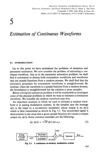
440. 424 5.1 Introduction
This is double sideband, suppressed carrier, amplitude modulation
(DSB-SC-AM).
s(t, a(t)) = V2P [1 + ma(t)] sin wet.
This is conventional DSB-AM with a residual carrier component.
s(t, a(t)) = V2P sin [wet + ,Ba(t)].
This is phase modulation (PM).
(2)
(3)
The transmitted waveform is corrupted by a sample function of zero-
mean Gaussian noise process which is independent of the message process.
The noise is completely characterized by its covariance function Kn(t, u).
Thus, for the system shown in Fig.S.l, the received signal is
r(t) = s(t, a(t)) + n(t), (4)
The simple system illustrated is not adequate to describe many problems
of interest. The first step is to remove the no-memory restriction. A
modulation system with memory is shown in Fig. 5.2. Here, h(t, u)
represents the impulse response of a linear, not necessarily time-invariant,
filter. Examples are the following:
1. The linear system is an integrator and the no-memory device is a
phase modulator. In this case the transmitted signal is
s(t, x(t)) = V2P sin [wet + I:. a(u) du]. (5)
This is frequency modulation (FM).
2. The linear system is a realizable time-invariant network and the
no-memory device is a phase modulator. The transmitted signal is
s(t, x(t)) = v2P sin [Wet + I:. h(t - u) a(u) dul (6)
This is pre-emphasized angle modulation.
Figures 5.1 and 5.2 describe a broad class of analog modulation systems
which we shall study in some detail. We denote the waveform of interest,
a(t), as the message. The message may come from a variety of sources. In
h(t, u)
Linear filter
Fig. S.l A modulation system with memory.

441. Typical Systems 42J
commercial FM it corresponds to music or speech. In a satellite telemetry
system it might correspond to analog data from a sensor (e.g., temperature
or attitude).
The waveform estimation problem occurs in a number of other areas.
If we remove the modulator in Fig. 5.1,
r(t) = a(t) + n(t), T1 ~ t ~ T1• (7)
If a(t) represents the position of some object we are trying to track in the
presence of measurement noise, we have the simplest form of the control
problem.
Many more complicated systems also fit into the model. Three are
shown in Fig. 5.3. The system in Fig. 5.3a is an FM/FM system. This type
of system is commonly used when we have a number of messages to
transmit. Each message is modulated onto a subcarrier at a different
frequency, the modulated subcarriers are summed, and modulated onto
the main carrier. In the Fig. 5.3a we show the operations for a single
message. The system in Fig. 5.3b represents an FM modulation system
-J2Psin(wet+ J:z(u)du)
'
z(t)
a(t)
(a)
(b)
Known linear
time-varying
channel
r-------------1
I I
sin Wet ------;
1
--;;.(. I
I I
I I
L-------------...1
Unknown channel
(c)
n(t)
n(t)
r(t)
r(t)
Fig. 5.3 Typical systems: (a} an FM/FM system; (b) transmission through varying
channel; (c) channel measurement.

442. 426 5.2 Derivation of Estimator Equations
transmitting through a known linear time-varying channel. In Fig. 5.3c
the channel has an impulse response that depends on the random process
a(t). The input is a deterministic signal and we want to estimate the
channel impulse response. Measurement problems of this type arise
frequently in digital communication systems. A simple example was
encountered when we studied the Rayleigh channel in Section 4.4. Other
examples will arise in Chapters 11.2 and 11.3. Note that the channel
process is the "message" in this class of problems.
We see that all the problems we have described correspond to the first
level in the hierarchy described in Chapter I. We referred to it as the
known signal-in-noise problem. It is important to understand the meaning
of this description in the context of continuous waveform estimation. If
a(t) were known, then s(t, a(t)) would be known. In other words, except
for the additive noise, the mapping from a(t) to r(t) is deterministic.
We shall find that in order to proceed it is expedient to assume that a(t)
is a sample function from a Gaussian random process. In many cases this
is a valid assumption. In others, such as music or speech, it is not.
Fortunately, we shall find experimentally that if we use the Gaussian
assumption in system design, the system will work well for many non-
Gaussian inputs.
The chapter proceeds in the following manner. In Section 5.2 we derive
the equations that specify the optimum estimate a(t). In Section 5.3 we
derive bounds on the mean-square estimation error. In Section 5.4 we
extend the results to vector messages and vector received signals. In
Section 5.5 we solve the nonrandom waveform estimation problem.
The purpose ofthe chapter is to develop the necessary equations and to
look at some of the properties that can be deduced without solving them.
A far more useful end result is the solutions of these equations and the
resulting receiver structures. In Chapter 6 we shall study the linear modula-
tion problem in detail. In Chapter 11.2 we shall study the nonlinear
modulation problem.
S.l DERIVATION OF ESTIMATOR EQUATIONS
In this section we want to solve the estimation problem for the type of
system shown in Fig. 5.1. The general category of interest is defined by the
property that the mapping from a(t) to s(t, a(t)) is a no-memory trans-
formation.
The received signal is
r(t) = s(t, a(t)) + n(t), (8)

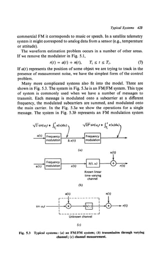
443. No-Memory Modulation Systems 427
By a no-memory transformation we mean that the transmitted signal at
some time t0 depends only on a(t0) and not on the past of a(t).
5.2.1 No-Memory Modulation Systems. Our specific assumptions are the
following:
I. The message a(t) and the noise n(t) are sample functions from
independent, continuous, zero-mean Gaussian processes with covariance
functions Ka(t, u) and Kn(t, u), respectively.
2. The signal s(t, a(t)) has a derivative with respect to a(t). As an
example, for the DSB-SC-AM signal in (1) the derivative is
os(t, a(t)) V2P .
oa(t) = sm wet. (9)
Clearly, whenever the transformation s(t, a(t)) is a linear transformation,
the derivative will not be a function of a(t). We refer to these cases as
linear modulation schemes. For PM
os(t, a(t)) . ;-
oa(t) = v 2P fi cos (wet + fia(t)). (10)
The derivative is a function of a(t). This is an example of a nonlinear
modulation scheme. These ideas are directly analogous to the linear
signaling and nonlinear signaling schemes in the parameter estimation
problem.
As in the parameter estimation case, we must select a suitable criterion.
The mean-square error criterion and the maximum a posteriori probability
criterion are the two logical choices. Both are conceptually straightforward
and lead to identical answers for linear modulation schemes.
For nonlinear modulation schemes both criteria have advantages and
disadvantages. In the minimum mean-square error case, if we formulate
the a posteriori probability density of a(t) over the interval [Tt, T,] as a
Gaussian-type quadratic form, it is difficult to find an explicit expression
for the conditional mean. On the other hand, if we model a(t) as a com-
ponent of a vector Markov process, we shall see that we can find a
differential equation for the conditional mean that represents a formal
explicit solution to the problem. This particular approach requires back-
ground we have not developed, and we defer it until Chapter II.2. In the
maximum a posteriori probability criterion case we are led to an integral
equation whose solution is the MAP estimate. This equation provides a
simple physical interpretation of the receiver. The MAP estimate will turn
out to be asymptotically efficient. Because the MAP formulation is more
closely related to our previous work, we shall emphasize it.t
t After we have studied the problem in detail we shall find that in the region in which
we get an estimator of practical value the MMSE and MAP estimates coincide.

444. 428 5.2 Derivation of Estimator Equations
To help us in solving the waveform estimation problem let us recall
some useful facts from Chapter 4 regarding parameter estimation.
In (4.464) and (4.465) we obtained the integral equations that specified
the optimum estimates of a set of parameters. We repeat the result. If
ar. a2, ... , aK are independent zero-mean Gaussian random variables,
which we denote by the vector a, the MAP estimates ai are given by the
simultaneous solution of the equations,
where
, 2 iTr os(z, A)J [ ( ) ( )] d
ai = Uj oA. • rg z - g z z,
Ti 1 A=a
ai2 ~ Var (aj),
ry(z) ~ I:.r Qn(z, u) r(u) du,
g(z) ~ rTf Qn(z, U) S(U, a) du,
JT,
and the received waveform is
r(t) = s(t, A) + n(t).
i = I, 2, ... , K, (II)
(12)
Ti::::; z::::; T1, (13)t
Ti::s;z::s;TI> (14)
Ti::::; t::::; Tr. (15)
Now we want to apply this result to our problem. From our work in
Chapter 3 we know that we can represent the message, a(t), in terms of an
orthonormal expansion:
K
a(t) = I.i.m. ,L ai 1/J;(t),
K-co i=l
where the if;i(t) are solutions to the integral equation
and
iT!
ai = a(t) if;i(t) dt.
Tt
The ai are independent Gaussian variables:
E(ai) = 0
and
(16)
(17)
(18)
(19)
(20)
Now we consider a subclass of processes, those that can be represented
by the first K terms in the orthonormal expansion. Thus
K
aK(t) = ,L ai if;i(t), (21)
i =1
t Just as in the colored noise discussions of Chapter 4, the end-points must be treated
carefully. Throughout Chapter 5 we shall include the end-points in the interval.

445. No-Memory Modulation Systems 429
Our logic is to show how the problem of estimating aK(t) in (21) is
identical to the problem we have already solved of estimating a set of K
independent parameters. We then let K ~ oo to obtain the desired result.
An easy way to see this problem is identical is given in Fig. 5.4a. If we
look only at the modulator, we may logically write the transmitted signal
as
(22)
By grouping the elements as shown in Fig. 5.4b, however, we may
logically write the output as s(t, A). Clearly the two forms are equivalent:
s(t, A) = s(t, ~~ A1 if11(t)).
Waveform generator
(conceptual)
(a)
Set of orthogonal function
multipliers and summer
(identical to section to the
right of dotted line in (a))
(b)
s(t,A)
s(t,aK(t))
K
(23)
=s(t,~ Ar./llt))
t=d
Modulator
Fig. 5.4 Equivalence of waveform representation and parameter representation.

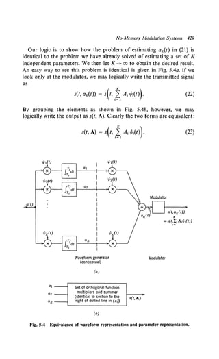
446. 430 5.2 Derivation of Estimator Equations
We define the MAP estimate of aK(t) as
K
aK(t) = L Gr ~r(t), (24)
r=l
We see that aK(t) is an interval estimate. In other words, we are estimating
the waveform aK(t) over the entire interval T1 ::5: t ::5: T1 rather than the
value at a single instant of time in the interval. To find the estimates of the
coefficients we can use (11).
Looking at (22) and (23), we see that
Bs(z, A) Bs(z, aK(z))
BAr BAr
Bs(z, aK(z) BaK(z)
BaK(z) · 8:4;
where the last equality follows from (21). From (11)
, JT' Bs(z, aK(z))l .1
.()[ () ( ]d
Or = f.Lr 0 ( ) 'f'r Z r9 Z - g z) Z,
Tt QK Z aK(Z)=4K(Z)
r = 1, 2, ... , K.
Substituting (26) into (24) we see that
or
(25)
(26)
(27)
In this form it is now easy to let K--+ oo. From Mercer's theorem in
Chapter 3
K
lim Lf.Lr ~r(t) ~r(z) = Ka(t, z).
K-+oo r=l
(29)
Now define
a(t) = l.i.m. aK(t), (30)
K-oo

447. No-Memory Modulation Systems 431
The resulting equation is
A rTf os(z, a(z))
a(t) = JT, oa(z) Ka(t, z)[rg(Z) - g(z)] dz, 1; 5 t 5 T1, (31)t
where
J
TI
rg(Z) = Qn(z, u) r(u) du,
Tt
T1 5 z 5 T1, (32)
and
iT!
g(z) = Qn(Z, U) S(U, a(u)) du,
T,
T1 5 z 5 T1• (33)
Equations 31, 32, and 33 specify the MAP estimate of the waveform
a(t). These equations (and their generalizations) form the basis of our
study of analog modulation theory. For the special case in which the
additive noise is white, a much simpler result is obtained. If
Kn(t, u) = ~0 8(t - u), (34)
then
2
Qn(t, u) = No 8(t - u).
Substituting (35) into (32) and (33), we obtain
2
rg(z) = No r(z)
and
g(z) = ~0 s(z, a(z)).
Substituting (36) and (37) into (31), we have
"( ) 2 rTf K ( ) os(z, a(z)) [ ( ) ( "( ))] d
a t = No JT, a t, z oa(z) r z - s z, a z z,
(35)
(36)
(37)
11 5 t 5 T1•
(38)
Now the estimate is specified by a single nonlinear integral equation.
In the parameter estimation case we saw that it was useful to interpret
the integral equation specifying the MAP estimate as a block diagram.
This interpretation is even more valuable here. As an illustration, we
consider two simple examples.
t The results in (31)-(33) were first obtained by Youla (1]. In order to simplify the
notation we have made the substitution
os(z, d(z)) £ os(z, a(z))l .
CJd(z) Ba(z) a(z) = a(Z)

448. 432 5.2 Derivation of Estimator Equations
r(t) +
s(t,a(t))
iJs(t, ti(t))
aa(tJ
Linear
nonrealizable
filter
a(t)
Ci(t)
Fig. 5.5 A block diagram of an unrealizable system: white noise.
Example 1. Assume that
T, = - oo, T1 = oo,
K.(t, u) = K.(t - u),
No
K.(t, u) = 2 ll(t - u).
In this case (38) is appropriate.t Substituting into (38), we have
• 2 J"' {os(z d(z)) }
a(t) = No _., K.(t - z) o~(z) [r(z) - s(z, d(z))] dz, - 00 < t < oo.
(39)
(40)
(41)
(42)
We observe that this is simply a convolution of the term inside the braces with a linear
filter whose impulse response is Ka(.,.). Thus we can visualize (42) as the block diagram
in Fig. 5.5. Observe that the linear filter is unrealizable. It is important to emphasize
that the block diagram is only a conceptual aid in interpreting (42). It is clearly not
a practical solution (in its present form) to the nonlinear integral equation because
we cannot build the unrealizable filter. One of the problems to which we shall devote
our attention in succeeding chapters is finding a practical approximation to the block
diagram.
A second easy example is the nonwhite noise case.
Example 2. Assume that
T, = -co, T1 = oo,
K.(t, u) = Ka(t - u),
K.(t, u) = K.(t - u).
Now (43) and (45) imply that
Q.(t, u) = Q.(t - u)
(43)
(44)
(45)
(46)
As in Example 1, we can interpret the integrals (31), (32), and (33) as the block
diagram shown in Fig. 5.6. Here, Q.(-r) is an unrealizable time-invariant filter.
t For this case we should derive the integral equation by using a spectral representa-
tion based on the integrated transform of the process instead of a Karhunen-Loeve
expansion representation. The modifications in the derivation are straightforward
and the result is identical; therefore we relegate the derivation to the problems (see
Problem 5.2.6).

449. Modulation Systems with Memory 433
r(t) + B(t)
as(t,B(t))
aQ.(t)
s(t, B(t))
Fig. 5.6 A block diagram of an unrealizable system: colored noise.
Before proceeding we recall that we assumed that the modulator was a
no-memory device. This assumption is too restrictive. As we pointed out
in Section 1, this assumption excludes such common schemes as FM.
While the derivation is still fresh in our minds we can modify it to eliminate
this restriction.
5.2.2 Modulation Systems with Memoryt
A more general modulation system is shown in Fig. 5.7. The linear
system is described by a deterministic impulse response h(t, u). It may be
time-varying or unrealizable. Thus we may write
JTI
x(t) = h(t, u) a(u) du,
Tt
(47)
The modulator performs a no-memory operation on x(t),
s(t, x(t)) = s(t, J;'h(t, u) a(u) du)· (48)
a(t)
Fig. 5.7 Modulator with memory.
t The extension to include FM is due to Lawton [2), [3]. The extension to arbitrary
linear operations is due to Van Trees [4]. Similar results were derived independently
by Rauch in two unpublished papers [5), [6).

450. 434 5.2 Derivation of Estimator Equations
As an example, for FM,
x(t) = d, r a(u) du,
JT,
where d1 is the frequency deviation. The transmitted signal is
s(t, x(t)) = V2P sin (wet + d1J:, a(u) du)·
(49)
(50)
Looking back at our derivation we see that everything proceeds identically
until we want to take the partial derivative with respect to A, in (25).
Picking up the derivation at this point, we have
os(z, A) os(z, xK(z))
oA, oA,
os(z, xK(z)) oxK(z).
OXK(z) """"'8A;'
(51)
but
iTt
= h(z, y) .p,(y) dy.
T,
(52)
It is convenient to give a label to the output of the linear operation when
the input is a(t). We define
iTt
XK(t) = h(t, Y) aK(Y) dy.
Tt
(53)
It should be observed that .XK(t) is not defined to be the MAP estimate of
xK(t). In view of our results with finite sets of parameters, we suspect that
it is. For the present, however, it is simply a function defined by (53)
From (11},
a, = 11-r I:' os~~~~~z)) (f:.'h(z, y) .p,(y) dy)<rg(Z) - g(z)) dz. (54)
As before,
K
aK(t) = L: a, .p,(t), (55)
r= 1

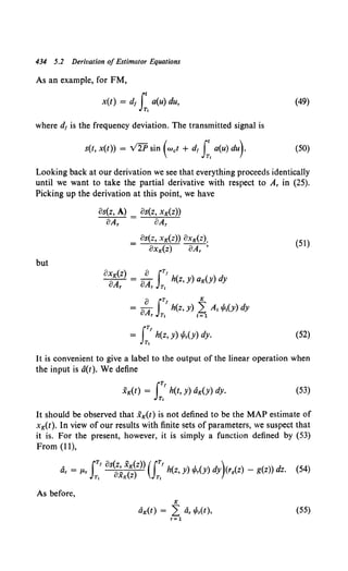
451. Modulation Systems with Memory 435
and from (54),
A IT' os(z, .XK(z)) {IT' [f ] }
OK(t) = T, OXK(z) T; h(z, y) r..S f-1-r ,P,(t) ,P,(y) dy
x [rg{z) - g(z)] dz. (56)
Letting K--+ oo, we obtain
Tt
A ff os(z, i(z))
a(t) = dy dz ci(z) h(z, y) Ka(t, y)[r9(z) - g(z)],
Tt
(57)
where r9(z) and g(z) were defined in (32) and (33) [replace d(u) by i(u)].
Equation 57 is similar in form to the no-memory equation (31). If we care
to, we can make it identical by performing the integration with respect to
yin (57)
ITt
h(z, y) Ka(t, y) dy Q ha(z, t)
T,
(58)
so that
A IT' os(z, i(z))
a(t) = dz r-q ) ha(z, t)(rg(z) - g(z)) dz,
T, (,X Z
Thus the block diagram we use to represent the equation is identical in
structure to the no-memory diagram given in Fig. 5.8. This similarity in
structure will prove to be useful as we proceed in our study of modulation
systems.
r(t) +
+
s(t,x(t))
Fig. 5.8 A block diagram.

452. 436 5.2 Derivation of Estimator Equations
4 h(-T)
®
Fig. 5.9 Filter interpretation.
An interesting interpretation of the filter ha(z, t) can be made for the
case in which Ti = -oo, T1 = oo, h(z, y) is time-invariant, and a(t) is
stationary. Then
ha(z, t) = J_'""' h(z - y) Ka(t - y) dy = ha(z- t). (60)
We see that ha(z - t) is a cascade of two filters, as shown in Fig. 5.9. The
first has an impulse response corresponding to that of the filter in the
modulator reversed in time. This is familiar in the context of a matched
filter. The second filter is the correlation function.
A final question of interest with respect to modulation systems with
memory is: Does
x(t) = x(t)? (61)
In other words, is a linear operation on a MAP estimate of a continuous
random process equal to the MAP estimate of the output of the linear
operation? We shall prove that (61) is true for the case we have just
studied. More general cases follow easily. From (53) we have
IT!
x(-r) = h(-r, t) a(t) dt.
T,
(62)
Substituting (57) into (62), we obtain
-c )= Jrl os(z, x(z)) [ ( ) _ ( )]
X T c. -c ) rg Z g Z
Ta uX Z
x [[!h('• t) h(z, y) K,(t, y) dt dy] dz. (63)

453. Derivation 437
We now want to write the integral equation that specifies .i{7') and
compare it with the right-hand side of(63). The desired equation is identical
to (31), with a(t) replaced by x(t). Thus
- rf os(z, x(z))
X(T) = JT, oi(z) K:b. z)[rg(z) - g(z)] dz. (64)
We see that .X(T) = i(T) if
Tt
JJh(T, t) h(z, y) Ka(t, y) dt dy = K:x(7', z), T; ~ T, z ~ T,; (65)
T;
but
Kx(7', z) Q E[x(T) x(z)] = E[f:.' h(T, t) a(t) dt J:.' h(z, y) a(y) dy]
Tt
= ffh(T, t) h(z, y) Ka(t, y) dt dy, Ti ~ T, z ~ T1, (66)
Tt
which is the desired result. Thus we see that the operations of maximum
a posteriori interval estimation and linear filtering commute. This result
is one that we might have anticipated from the analogous results in Chapter
4 for parameter estimation.
We can now proceed with our study of the characteristics of MAP
estimates of waveforms and th~.; structure of the optimum estimators.
The important results of this section are contained in (31), (38), and (57).
An alternate derivation of these equations with a variational approach is
given in Problem 5.2.1.
5.3 A LOWER BOUND ON THE MEAN-SQUARE ESTIMATION ERRORt
In our work with estimating finite sets of variables we found that an
extremely useful result was the lower bound on the mean-square error
that any estimate could have. We shall see that in waveform estimation
such a bound is equally useful. In this section we derive a lower bound on
the mean-square error that any estimate of a random process can have.
First, define the error waveform
a.(t) = a(t) - a(t) (67)
and
(68)
t This section is based on Van Trees [7].

454. 438 5.3 Lower Bound on the Mean-Square Estimation Error
where T f! T1 - T1• The subscript I emphasizes that we are making an
interval estimate. Now e1 is a random variable. We are concerned with its
expectation,
{IT! oo oo }
nr f! TE(ei) = E T, ~~ (at - ai) tPt(t) /~1 (aj - aj) !fit) dt . (69)
Using the orthogonality of the eigenfunctions, we have
00
giT = L E(a1 - a1) 2 • (70)
I= 1
We want to find a lower bound on the sum on the right-h,and side.
We first consider the sum L:f= 1 E(a1 - a1) 2 and then let K-+ oo. The
problem of bounding the mean-square error in estimating K random
variables is familiar to us from Chapter 4.
From Chapter 4 we know that the first step is to find the information
matrix JT, where
JT = JD + Jp, (71a)
Jv,J = -E[82
ln A(A)l
8A1 8A1
(71b)
and
JP,J = -E[82
lnpa(Al
8A1 8A1
(7lc)
After finding JT, we invert it to obtain JT - 1. Throughout the rest of this
chapter we shall always be interested in JT so we suppress the subscript T
for convenience. The expression for ln A(A) is the vector analog to (4.217)
Tt
1n A(A) = II[r(t) - ! s(t, A)] Qn(t, u) s(u, A) dt du (72a)
or, in terms of aK(t),
Tt
Tt
In A(aK(t)) = II[r(t) - -! s(t, aK(t))] Qn(t, u) s(u, aK(u)) dt du.
Tt
From (19) and (20)
K [ A 2
1 ]
lnpa(A) = L - ~- 2ln (27T) .
1=1 p.,
(72b)
(72c)
Adding (72b) and (72c) and differentiating with respect to A~o we obtain
8(lnpa(A) + ln A(aK(t))]
8A1
A1 ITt 8s(t, aK(t)) JTt
-- + dt ,P1(t) 0 ( ) Qn(t, u)[r(u) - s(u, aK(u))] du.
fLI Tt UK ( T,
(72d)

455. Derivation 439
Differentiating with respect to A1 and including the minus signs, we have
Tr
r = Su E IId d.1
.( ) .1
. ( ) os(t, aK(t)) Q ( ) os(u, aK(u))
JIJ + t U 'f'i t 'f'i U , ( } n t, U , ( )
~ ~~ ~u
T,
+ terms with zero expectation. (73)
Looking at (73), we see that an efficient estimate will exist only when the
modulation is linear (see p. 84).
To interpret the first term recall that
«>
Ka(t, u) = Lp.1 I/J1(t) I/J1(u), (74)
1=1
Because we are using only K terms, we define
K
KaK(t, u) ~ L P-1 1/J,(t) 1/J,(u), T1 :s; t, u :s; T1• (75)
1=1
The form of the first term in (73) suggests defining
K }
QaK(t, u) = L - I/J1(t) I/J1(u),
1=1 1-'t
(76)
We observe that
JT1 K
T, QaK(t, u) KaK(u, z) du = 1~ I/J1(t) I/J1(z), T1 :s; t, z :s; T1. (77)
Once again, QaK(t, u) is an inverse kernel, but because the message a(t)
does not contain a white noise component, the limit of the sum in (76) as
K-+ oo will not exist in general. Thus we must eliminate QaK(t, u) from
our solution before letting K-+ oo. Observe that we may write the first
term as
Tf
~: = IIQaK(t, u) I/J1(t) .Plu) dt du, (78)
Tt
so that if we define
J (t u) 6. Q (t u) + E [os(t, aK(t)) Q (t u) os(u, aK(u))] (79)
K ' - aK ' OaK(t) n ' OaK(U)
we can write the elements of the J matrix as
Tf
J11 = IIJK(t, u) .Plt) .Plu) dt du, i,j = l, 2, ... , K. (80)
T,

456. 440 5.3 Lower Bound on the Mean-Square Estimation Error
Now we find the inverse matrix J- 1• We can show (see Problem 5.3.6) that
Tf
P1 = IIJK - 1(t, u) 1/lt(t) 1/J;(u) dt du (81)
T,
where the function Jx - 1(t, u) satisfies the equation
(82)
(Recall that the superscript ij denotes an element in J- 1.) We now want
to put (82) into a more usable form.
If we denote the derivative of s(t, aK(t)) with respect to aK(t) as
d.(t, aK(t)}, then
E [os~~={t~)) os~~K(~~u))] = E[d,(t, aK(t)) d,(u, aK(u))]
~ Rd,K(t, u). (83a)
Similarly
[8s(t, a(t)) 8s(u, a(u))] _ b.
E oa(t) oa(u) - E[d,(t, a(t)) d.(u, a(u))] _ Rd.(t, u). (83b)
Therefore
(84)
Substituting (84) into (82), multiplying by KaK(z, x}, integrating with
respect to z, and letting K ---J>- oo, we obtain the following integral equation
for J- 1(t, x),
J- 1(t, x) + I:'du I:'dz J- 1(t, u) Rd.(u, z) Qn(u, z) Ka(z, x) (85)
= Ka(t, x), T, :::; t, X :::; T,.
From (2.292) we know that the diagonal elements of J -l are lower bounds
on the mean-square errors. Thus
E[(a1 - a1
) 2] ;::: J". (86a)
Using (81) in (86a) and the result in (70), we have
Tr
nl ;::: 1~~ ~~IIJK - 1(t, u) 1/Jt(t) 1/J,(u) dt du (86b)
T,
or, using (3.128),
(87)

457. Information Kernel 441
Therefore to evaluate the lower bound we must solve (85) for J-1(1, x)
and evaluate its trace. By analogy with the classical case, we refer to
J(t, x) as the information kernel.
We now want to interpret (85). First consider the case in which there is
only a white noise component so that,
2
Qn(t, u) = No S(t - u). (88)
Then (85) becomes
J- 1(1, x) + IT' du ~ J- 1(t, u) Ra,(u, u) K4(u, x) = K4(t, x),
Tt 0
T1 :::;; t, x :::;; T1. (89)
The succeeding work will be simplified if Ra.(t, t) is a constant. A sufficient,
but not necessary, condition for this to be true is that d,(t, a(t)) be a
sample function from a stationary process. We frequently encounter
estimation problems in which we can approximate Ra.(t, t) with a constant
without requiring d,(t, a(t)) to be stationary. A case of this type arises
when the transmitted signal is a bandpass waveform having a spectrum
centered around a carrier frequency we; for example, in PM,
s(t, a(t)) = V2P sin [wet + ,Ba(t)]. (90)
Then
os(t a(t)) _;-
d,(t, a(t)) = o~(t) = v 2P ,8 cos [wet + ,8 a(t)] (91)
and
Ra.(t, u) = ,82PE4{Cos [we(t - u) + ,8 a(t) - ,8 a(u)]
+ cos [w0 (t + u) + ,8 a(t) + ,8 a(u)]}. (92)
Letting u = t, we observe that
Ra,(t, t) = ,82P(l + Ea{cos [2wet + 2,8 a(t)]}). (93)
We assume that the frequencies contained in a(t) are low relative to we.
To develop the approximation we fix tin (89). Then (89) can be represented
as the linear time-varying system shown in Fig. 5.10. The input is a
function of u, J- 1(t, u). Because Ka(u, x) corresponds to a low-pass filter
and K4(t, x), a low-pass function, we see that J- 1(t, x) must be low-pass
and the double-frequency term in Ra.(u, u) may be neglected. Thus we
can make the approximation
(94)
to solve the integral equation. The function R:.(O) is simply the stationary
component of Ra,(t, t). In this example it is the low-frequency component.

458. 442 5.3 Lower Bound on the Mean-Square Estimation Error
(t fixed)
T;:Su :STt
r---------------,
2
NoRd (u, u)
low-pass filter
L---------------
Fig. 5.10 Linear system interpretation.
(Note that Rt(O) = Ra.(O) when d.(t, a(t)) is stationary.) For the cases in
which (94) is valid, (89) becomes
-1 ) 2R:.(O) lT' d -1( ) ( )
J (t, X + -w;- JT, UJ t, u) Ka(U, X = Ka t, X , {9S)
Tl ~ t, X~ T,,
which is an integral equation whose solution is the desired function. From
the mathematical viewpoint, (95) is an adequate final result.
We can, however, obtain a very useful physical interpretation of our
result by observing that (95) is familiar in a different context. Recall the
following linear filter problem (see Chapter 3, p. 198).
r(t) = a(t) + n1(t), (96)
where a(t) is the same as our message and n1(t) is a sample function from
a white noise process (N1/2, double-sided). We want to design a linear
filter h(t, x) whose output is the estimate of a(t) which minimizes the
mean-square error. This is the problem that we solved in Chapter 3. The
equation that specifies the filter h0 (t, x) is
N1 IT'
T ho(t, x) + ha(t, u) Ka(u, x) du = Ka(t, x),
Tt
where N1/2 is the height of the white noise. We see that if we let
No
Nl = R:.(O)
then
r 1(t, x) = z%:~(0) ho(t, x).
(98)
(99)

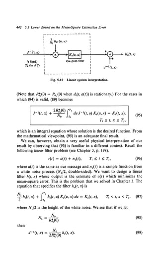
459. Equivalent Linear Systems 443
The error in the linear filtering problem is
I IT' N I iT'
'I = T Tha(x, x) dx = T J-1
(x, x) dx,
Tt T1
(100)
Our bound for the nonlinear modulation problem corresponds to the
mean-square error in the linear filter problem except that the noise level
is reduced by a factor R3,(0).
The quantity R3,(0) may be greater or less than one. We shall see in
Examples 1 and 2 that in the case of linear modulation we can increase
Ra,(O) only by increasing the transmitted power. In Example 3 we shall see
that in a nonlinear modulation scheme such as phase modulation we can
increase Rt,(O) by increasing the modulation index. This result corresponds
to the familiar PM improvement.
It is easy to show a similar interpretation for colored noise. First
define an effective noise whose inverse kernel is,
Qne(t, u) = Ra.(t, u) Qn(t, u). (101)
Its covariance function satisfies the equation
J
T, Kne(t, u) Qne(u, z) du = S(t - z),
Tt
11 < t, z < T1• (102)
Then we can show that
JTI
J- 1(u, z) = Kne(u, x) h0 (X, z) dx,
Tt
(103)
where h.(x, z) is the solution to,
J
TI
[Ka(X, t) + Kne(X, t)] h0(t, z) dt = Ka(X, z),
Tt
(104)
This is the colored noise analog to (95).
Two special but important cases lead to simpler expressions.
Case 1. J- 1(t, u) = J- 1(t - u). Observe that when J- 1(t, u) is a function
only of the difference of its two arguments
r 1(t, t) = J- 1(t- t) = J- 1(0). (105)
Then (87) becomes,
'I;:::J-1(0). (106)
If we define
a-1(w) = s:"' J- 1(T)e-ioJt dT, (107)
then
ei = a-1(w) -·
I"' dw
-CXl 27T
(108)

460. 444 5.3 Lower Bound on the Mean-Square Estimation Error
A further simplification develops when the observation interval includes
the infinite past and future.
Case 2. Stationary Processes, Infinite Interval.t Here, we assume
Then
T1 = -oo,
T1 = oo,
Ka(t, u) = Ka(t - u),
Kn(t, u) = Kn(t - u),
Rd.(t, u) = Rd.(t - u).
J- 1(t, u) = J- 1(t - u).
The transform of J(T) is
'J(w) = J:"'J(T)e-ion dT.
Then, from (82) and (85),
a-1
(w) = alw) = [sa~w) + Sd,(w) ® Sn~w)] -
1
(where ® denotes convolutiont) and the resulting error is
g1 ~ s:"' [sa~w) + Sd.(w) ® Sn~w)] -
1
~=·
Several simple examples illustrate the application of the bound.
Example 1. We assume that Case 2 applies. In addition, we assume that
s(t, a(t)) = a(t).
(109)
(110)
(Ill)
(112)
(113)
(114)
(115)
(116)
(117)
(118)
Because the modulation is linear, an efficient estimate exists. There is no carrier so
os(t, a(t))foa(t) = 1 and
Sd,(w) = 2wS(w).
Substituting into (117), we obtain
~ - I"' Sa(w) s.(w) dw
1 - _,. Sa(w) + S.(w) 2w.
(119)
(120)
The expression on the right-hand side of (120) will turn out to be the minimum mean-
square error with an unrealizable linear filter (Chapter 6). Thus, as we would expect,
the efficient estimate is obtained by processing r(t) with a linear filter.
A second example is linear modulation onto a sinusoid.
Example 2. We assume that Case 2 applies and that the carrier is amplitude-
modulated by the message,
s(t, a(t)) = V2Pa(t) sin wet, (121)
t See footnote on p. 432 and Problem 5.3.3.
t We include 1/2w in the convolution operation when w is the variable.

461. Examples 445
where a(t) is low-pass compared with we. The derivative is,
fJs(t, a(t)) _ .;2p .
fJa(t) - sm wet. (122)
For simplicity, we assume that the noise has a flat spectrum whose bandwidth is
much larger than that of a(t). It follows easily that
~ f"' Sa(w) dw
1 = -., 1 + Sa(w)(2P/No) 2:;"
(123)
We can verify that an estimate with this error can be obtained by multiplying r(t) by
v2/P sin wet and passing the output through the same linear filter as in Example 1.
Thus once again an efficient estimate exists and is obtained by using a linear system
at the receiver.
Example 3. Consider a phase-modulated sine wave in additive white noise. Assume
that a(t) is stationary. Thus
s(t, a(t)) = v2P sin (wet + .B a(t)], (124)
OS~~~~)) = V2P .a cos (wet + .a a(t)] (125)
and
No
Kn(t, u) = T 8(t-u).
Then, using (92), we see that
R:,(O) = P.B2 •
• By analogy with Example 2 we have
~1 > f"' Sa(w) dw.
- -., 1 + Sa(w)(2P.B2 /No) 21T
(126)
(127)
(128)
In linear modulation the error was only a function of the spectrum of
the message, the transmitted power and the white noise level. For a given
spectrum and noise level the only way to decrease the mean-square error
is to increase the transmitted power. In the nonlinear case we see that by
increasing {3, the modulation index, we can decrease the bound on the
mean-square error. We shall show that as P/N0 is increased the mean-
square error of a MAP estimate approaches the bound given by (128).
Thus the MAP estimate is asymptotically efficient. On the other hand, if{3
is large and P/N0 is decreased, any estimation scheme will exhibit a
"threshold." At this point the estimation error will increase rapidly and
the bound will no longer be useful. This result is directly analogous to that
obtained for parameter estimation (Example 2, Section 4.2.3). We recall
that if we tried to make {3 too large the result obtained by considering the
local estimation problem was meaningless. In Chapter 11.2, in which we
discuss nonlinear modulation in more detail, we shall see that an analogous
phenomenon occurs. We shall also see that for large signal-to-noise ratios
the mean-square error approaches the value given by the bound.

462. 446 5.4 Multidimensional Waveform Estimation
The principal results of this section are (85), (95), and (97). The first
equation specifies J- 1(t, x), the inverse of the information kernel. The
trace of this inverse kernel provides a lower bound on the mean-square
interval error in continuous waveform estimation. This is a generalization
of the classical Cramer-Rao inequality to random processes. The second
equation is a special case of (85) which is valid when the additive noise is
white and the component of d.(t, a(t)) which affects the integral equation
is stationary. The third equation (97) shows how the bound on the mean-
square interval estimation error in a nonlinear system is identical to the
actual mean-square interval estimation error in a linear system whose
white noise level is divided by R:,(O).
In our discussion of detection and estimation we saw that the receiver
often had to process multiple inputs. Similar situations arise in the wave-
form estimation problem.
5.4 MULTIDIMENSIONAL WAVEFORM ESTIMATION
In Section 4.5 we extended the detection problem to M received signals.
In Problem 4.5.4 of Chapter 4 it was demonstrated that an analogous
extension could be obtained for linear and nonlinear estimation of a single
parameter. In Problem 4.6.7 of Chapter 4 a similar extension was obtained
for multiple parameters. In this section we shall estimate N continuous
messages by using M received waveforms. As we would expect, the deriva-
tion is a simple combination of those in Problems 4.6.7 and Section 5.2.
It is worthwhile to point out that all one-dimensional concepts carry
over directly to the multidimensional case. We can almost guess the form of
the particular results. Thus most of the interest in the multidimensional
case is based on the solution of these equations for actual physical
problems. It turns out that many issues not encountered in the scalar case
must be examined. We shall study these issues and their implications in
detail in Chapter 11.5. For the present we simply derive the equations
that specify the MAP estimates and indicate a bound on the mean-square
errors.
Before deriving these equations, we shall find it useful to discuss several
physical situations in which this kind of problem occurs.
5.4.1 Examples of Multidimensional Problems
Case 1. Multilevel Modulation Systems. In many communication systems
a number ofmessages must be transmitted simultaneously. In one common
method we perform the modulation in two steps. First, each of the

463. Examples of Multidimensional Problems 447
Fig. 5.11 An FM/FM system.
messages is modulated onto individual subcarriers. The modulated sub-
carriers are then summed and the result is modulated onto a main carrier
and transmitted. A typical system is the FM/FM system shown in Fig. 5.11,
in which each message a1(t), (i = 1, 2, ... , N), is frequency-modulated
onto a sine wave of frequency w1• The w1 are chosen so that the modulated
subcarriers are in disjoint frequency bands. The modulated subcarriers are
amplified, summed and the result is frequency-modulated onto a main
carrier and transmitted.
Notationally, it is convenient to denote the N messages by a column
matrix,
[
a1(r)l
a2(r)
a(r) Q ; .
aN(r)
(129)
Using this notation, the transmitted signal is
s(t, a(r)) = V2Psin [wet+ d1c J:, z(u)du], (130)t
where
z(u) = I v2 gj sin [w;U + d,J ru a;(r) dr]. (131)
J=l JT,
t The notation s(t, a(T)) is an abbreviation for s(t; a(T), T. s T S t). The second
variable emphasizes that the modulation process has memory.

464. 448 5.4 Multidimensional Waveform Estimation
The channel adds noise to the transmitted signal so that the received
waveform is
r(t) = s(t, a(T)) + n(t). (132)
Here we want to estimate the N messages simultaneously. Because there
are N messages and one received waveform, we refer to this as anN x }-
dimensional problem.
FM/FM is typical of many possible multilevel modulation systems such
as SSB/FM, AM/FM, and PM/PM. The possible combinations are
essentially unlimited. A discussion of schemes currently in use is available
in [8).
Case 2. Multiple-Channel Systems. In Section 4.5 we discussed the use of
diversity systems for digital communication systems. Similar systems can
be used for analog communication. Figure 5.12 in which the message a(t)
is frequency-modulated onto a set of carriers at different frequencies is
typical. The modulated signals are transmitted over separate channels,
each of which attenuates the signal and adds noise. We see that there are
M received waveforms,
(i= 1,2, ... ,M), (133)
where
si(t, a(r)) = g; v2P; sin (Wet + dt, I:.a(u) du)· (134)
Once again matrix notation is convenient. We define
[
s1(t, a(r))l
s2(t, a(T))
s(t, a(T)) = .
sM(t, a(r))
(135)
--.fiii1 sin (w1t+ dttJ;,a(r)d'T)
Attenuator
Fig. 5.12 Multiple channel system.

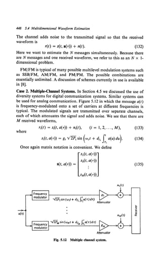
465. I
'
'
, ,
y
'
( Rooe;,;og
array
and
Then
I
Examples of Multidimensional Problems 449
I
I
X
Fig. 5.13 A space-time system.
n(t) = [:~:~]·
nM(t)
(136)
r(t) = s(t, a(T)) + n(t). (137)
Here there is one message a(t) to estimate and M waveforms are available
to perform the estimation. We refer to this as a 1 x M-dimensional
problem. The system we have shown is a frequency diversity system.
Other obvious forms of diversity are space and polarization diversity.
A physical problem that is essentially a diversity system is discussed in
the next case.
Case 3. A Space-Time System. In many sonar and radar problems the
receiving system consists of an array of elements (Fig. 5.13). The received
signal at the ith element consists of a signal component, s1
(t, a(T)), an
external noise term nE1(t), and a term due to the noise in the receiver
element, nRi(t). Thus the total received signal at the ith element is
(138)

466. 450 5.4 Multidimensional Waveform Estimation
We define
(139)
We see that this is simply a different physical situation in which we have
M waveforms available to estimate a single message. Thus once again we
have a 1 x M-dimension problem.
Case 4. N x M-Dimensional Problems. If we take any of the multilevel
modulation schemes of Case 1and transmit them over a diversity channel,
it is clear that we will have an N x M-dimensional estimation problem.
In this case the ith received signal, r1(t), has a component that depends on
N messages, a1(t), U = 1, 2, ... , N). Thus
i = 1, 2, ... , M. (140)
In matrix notation
r(t) = s(t, a(r)) + n(t). (141)
These cases serve to illustrate the types of physical situations in which
multidimensional estimation problems appear. We now formulate the
model in general terms.
5.4.2 Problem Formulationt
Our first assumption is that the messages a1(t), (i = 1, 2, ... , N), are
sample functions from continuous, jointly Gaussian random processes.
It is convenient to denote this set of processes by a single vector process
a(t). (As before, we use the term vector and column matrix interchange-
ably.) We assume that the vector process has a zero mean. Thus it is
completely characterized by an N x N covariance matrix,
Ka(t, u) ~ E[(a(t) aT(u))]
~[~~(~.:~;~-~~-~:"~_i ...~~;;~} (142)
Thus the ijth element represents the cross-covariance function between
the ith and jth messages.
The transmitted signal can be represented as a vector s(t, a(T)). This
vector signal is deterministic in the sense that if a particular vector sample
t The multidimensional problem for no-memory signaling schemes and additive
channels was first done in [9]. (See also [10].)

467. Derivation of Estimator Equations 451
function a(r) is given, s(t, a(r)) will be uniquely determined. The trans-
mitted signal is corrupted by an additive Gaussian noise n(t). The signal
available to the receiver is an M-dimensional vector signal r(t),
r(t) = s(t, a(r)) + n(t), (143)
or
[
r1
(t)l[s1
(t, a(r))l[n1
(t)l
r2(t) s2(t, a(r)) n2(t)
. = . + . '
. . .
. . .
rM(t) sM(t, a(r)) nM(t)
(144)
The general model is shown in Fig. 5.14.
We assume that the M noise waveforms are sample functions from
zero-mean jointly Gaussian random processes and that the messages and
noises are statistically independent. (Dependent messages and noises can
easily be included, cf. Problem 5.4.1.) We denote theM noises by a vector
noise process n(t) which is completely characterized by an M x M
covariance matrix K0 (t, u).
5.4.3 Derivation of Estimator Equations.
We now derive the equations for estimating a vector process. For
simplicity we shall do only the no-memory modulation case here. Other
cases are outlined in the problems.
The received signal is
r(t) = s(t, a(t)) + n(t), (145)
where s(t, a(t)) is obtained by a no-memory transformation on the vector
a(t). We also assume that s(t, a(t)) is differentiable with respect to each ai(t).
The first step is to expand a(t) in a vector orthogonal expansion.
K
a(t) = l.i.m. 2 ar~r(t),
K-+a:> r=l
(146)
n(t)
Fig. 5.14 The vector estimation model.

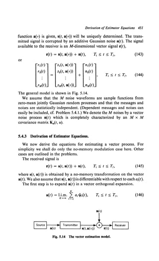
468. 452 5.4 Multidimensional Waveform Estimation
or
(147)
where the..jlr(t) are the vector eigenfunctions corresponding to the integral
equation
(148)
This expansion was developed in detail in Section 3.7. Then we find dr
and define
K
a(t) = u.m. L: ar..jlr(t).
K-.oo r=l
(149)
We have, however, already solved the problem of estimating a parameter
ar. By analogy to (72d) we have
0 [ln A(A) + lnpa (A)] = JT' osT(z, a(z)) [ ( ) - ( )] d - AT
"A "A rg z g z z ,
u r Ti u r J-Lr
(r = I, 2, ... ), (150)
where
(151)
and
g(z) ~ J:' Qn(z, u) s(u, a(u)) du. (152)
The left matrix in the integral in (150) is
osr(t, a(t)) = [os1(t, a(t)) :... j osM(t, a(t))].
oAr oAr ~ 1 oAr
(153)
The first element in the matrix can be written as
(154)
Looking at the other elements, we see that if we define a derivative
matrix
os1(t, a(t)) : : asM(t, a(t))
oa1(t) :· · ·: oa1(t)
·-----------
D(t, a(t)) ~ Va(t){sT(t, a(t))} = (155)
8~~(t-,-;(-t))-: i-~;~(;,-~(-t))
OaN(t) :• .. : OaN(t)

469. Lower Bound on the Error Matrix 453
we may write
BsT(t, a(t)) = .r. T( ) D( ( ))
BAr 't"r t t, a t , (156)
so that
8 [In A(A) +lnpa(A)] = rrl.jl/(z) D(z, a(z))[rg{z) - g(z)] dz - Ar. (157)
oAr JT, fLr
Equating the right-hand side to zero, we obtain a necessary condition on
the MAP estimate of Ar. Thus
iir = fLr J:'l.jl/(z) D(z, a(z))[rg{z) - g(z)] dz. (158)
Substituting (158) into (149), we obtain
a(t) = J:' L~ fLrl.jlr(t)jlrT(z)] D(z, a(z))[rg{z) - g(z)] dz. (159)
We recognize the term in the bracket as the covariance matrix. Thus
a(t) = rTr Ka(t, z) D(z, a(z))[rg{z) - g(z)] dz,
JT,
(160)
As we would expect, the form of these equations is directly analogous
to the one-dimensional case.
The next step is to find a lower bound on the mean-square error in
estimating a vector random process.
5.4.4 Lower Bound on the Error Matrix
In the multidimensional case we are concerned with estimating the
vector a(t). We can define an error vector
a(t) - a(t) = a,(t), (161)
which consists of N elements: a,,(t), a,2 (t), ... , a,N(t). We want to find
the error correlation matrix.
Now,
00 00
a(t)- a(t) = 2 (at - at)jl;(t) ~ 2 a., jl;(t). (162)
i= 1 i=l
Then, using the same approach as in Section 5.3, (68),
Re1 ~ ~ E u:ra,(t) a/(t) dt]
1 rTr K K
= T }~n:!, JT, dt ~~ 1~1l.jl1(t) E(a,,a,)l.jll(t). (163)

470. 454 5.4 Multidimensional Waveform Estimation
We can lower bound the error matrix by a bound matrix R8 in the sense
that the matrix R.1 - R8 is nonnegative definite. The diagonal terms in
R8 represent lower bounds on the mean-square error in estimating the
a1(t). Proceeding in a manner analogous to the one-dimensional case, we
obtain
1 JTf
RB = T J- 1(t, t) dt.
T,
(164)
The kernel J - 1(t, x) is the inverse of the information matrix kernel J(t, x)
and is defined by the matrix integral equation
J- 1(t, x) + JT' du JT' dz J- 1(t, u){E[D(u, a(u)) Qn(u, z) DT(z, a(z))]}Ka(z, x)
T, T,
= Ka(t, x), T1 :::; t, x :::; T1• (165)
The derivation of (164) and (165) is quite tedious and does not add
any insight to the problem. Therefore we omit it. The details are contained
in [11].
As a final topic in our current discussion of multiple waveform estima-
tion we develop an interesting interpretation of nonlinear estimation in the
presence of noise that contains both a colored component and a white
component.
5.4.5 Colored Noise Estimation
Consider the following problem:
r(t) = s(t, a(t)) + w(t) + n0 (t), (166)
Here w(t) is a white noise component (N0/2, spectral height) and nc(t) is
an independent colored noise component with covariance function
K0(t, u). Then
Kn(t, u) = ~0 S(t - u) + K0 (t, u). (167)
The MAP estimate of a(t) can be found from (31), (32), and (33)
A JT' os(u, a(u))
a(t) = Ka(t, u) 0'( ) [rg{u) - g(u)] du,
T, au
where
r(t) - s(t, a(t)) = JT' Kn(t, u)[rg(u) - g(u)] du,
T,
Substituting (167) into (169), we obtain
r(t) - s(t, a(t)) = I:.' [~o S(t- u) + Kc(t, u)] [r9(u) - g(u)] du. (170)

471. Colored Noise Estimation 455
We now want to demonstrate that the same estimate, a(t), is obtained
if we estimate a(t) and nc(t) jointly. In this case
( ) /:::,. [a(t) ]
at _ ()
nc t
(171)
and
K ( ) _ [Ka(t, u) 0 ]
a t, u - 0 Kc(t, u) • (172)
Because we are including the colored noise in the message vector, the
only additive noise is the white component
K,.(t, u) = ~0 S(t - u). {173)
To use (160) we need the derivative matrix
[
os(t, a(t))]
D(t, a(t)) = oait) . (174)
Substituting into (160), we obtain two scalar equations,
a(t) = f~1 !to Ka(t, u) os~d(:~u)) [r(u) - s(u, a(u)) - iic(u)] du,
T1 :s; t :s; T1, (175)
nc(t) = jT1;, K0(t, u)[r(u) - s(u, a(u)) - fic(u)] du, Tt :s; t :s; T,.
JT, 0
(176)
Looking at (168), (170), and (175), we see that a(t) will be the same in
both cases if
f~1 !to [r(u) - s(u, d(u)) - nc(u)][~o S(t - u) + Kc(t, u)]du
= r(t)- s(t, d(t)); (177)
but (177) is identical to (176).
This leads to the following conclusion. Whenever there are independent
white and colored noise components, we may always consider the colored
noise as a message and jointly estimate it. The reason for this result is that
the message and colored noise are independent and the noise enters into
r(t) in a linear manner. Thus theN x 1vector white noise problem includes
all scalar colored noise problems in which there is a white noise component.
Before summarizing our results in this chapter we discuss the problem
of estimating nonrandom waveforms briefly.

472. 456 5.5 Nonrandom Waveform Estimation
5.5 NONRANDOM WAVEFORM ESTIMATION
It is sometimes unrealistic to consider the signal that we are trying to
estimate as a random waveform. For example, we may know that each
time a particular event occurs the transmitted message will have certain
distinctive features. If the message is modeled as a sample function of a
random process then, in the processing of designing the optimum receiver,
we may average out the features that are important. Situations of this type
arise in sonar and seismic classification problems. Here it is more useful
to model the message as an unknown, but nonrandom, waveform. To
design the optimum processor we extend the maximum-likelihood estima-
tion procedure for nonrandom variables to the waveform case. An
appropriate model for the received signal is
r(t) = s(t, a(t)) + n(t), T1 ~ t ~ T1, (178)
where n(t) is a zero-mean Gaussian process.
To find the maximum-likelihood estimate, we write the ln likelihood
function and then choose the waveform a(t) which maximizes it. The ln
likelihood function is the limit of (72b) asK~ oo.
In A(a(t)) = J;'dt J~' du s(t, a(t)) Qn(t, u)[r(u) - ! s(u, a(u))], (179)
where Qn(t, u) is the inverse kernel of the noise. For arbitrary s(t, a(t))
the minimization of ln A(a(t)) is difficult. Fortunately, in the case of most
interest to us the procedure is straightforward. This is the case in which
the range of the function s(t, a(t)) includes all possible values of r(t). An
important example in which this is true is
r(t) = a(t) + n(t). (180)
An example in which it is not true is
r(t) = sin (wet + a(t)) + n(t). (181)
Here all functions in the range of s(t, a(t)) have amplitudes less than one
while the possible amplitudes of r(t) are not bounded.
We confine our discussion to the case in which the range includes all
possible values of r(t). A necessary condition to minimize In A(a(t))
follows easily with variational techniques:
IT, aE(t) dt{os~: a('jt)IT' Qn(t, u)[r(u) - s(u, dmzCu))] du} = 0 (182)
T, aml t T1
for every aE(t). A solution is
r(u) = s(u, amz(u)), (183)
because for every r(u) there exists at least one a(u) that could have mapped
into it. There is no guarantee, however, that a unique inverse exists. Once

473. Maximum Likelihood Estimation 457
again we can obtain a useful answer by narrowing our discussion.
Specifically, we shall consider the problem given by (180). Then
amz(U) = r(u). (184)
Thus the maximum-likelihood estimate is simply the received waveform.
It is an unbiased estimate of a(t). It is easy to demonstrate that the
maximum-likelihood estimate is efficient. Its variance can be obtained
from a generalization ofthe Cramer-Rao bound or by direct computation.
Using the latter procedure, we obtain
al ~ E{J;'[am1(t) - a(t)]2 dt}- (185)
It is frequently convenient to normalize the variance by the length of the
interval. We denote this normalized variance (which is just the average
mean-square estimation error) as ~mz:
~mz ~ E {~ J:.' [am1
(t) - a(t))2 dt}· (186)
Using (180) and (184), we have
}iT/
~mz = T K,.(t, t) dt.
T,
(187)
Several observations follow easily.
If the noise is white, the error is infinite. This is intuitively logical if we
think of a series expansion of a(t). We are trying to estimate an infinite
number of components and because we have assumed no a priori informa-
tion about their contribution in making up the signal we weight them
equally. Because the mean-square errors are equal on each component, the
equal weighting leads to an infinite mean-square error. Therefore to make
the problem meaningful we must assume that the noise has finite energy
over any finite interval. This can be justified physically in at least two ways:
I. The receiving elements (antenna, hydrophone, or seismometer) will
have a finite bandwidth;
2. If we assume that we know an approximate frequency band that
contains the signal, we can insert a filter that passes these frequencies
without distortion and rejects other frequencies.t
t Up to this point we have argued that a white noise model had a good physical basis.
The essential point of the argument was that if the noise was wideband compared with
the bandwidth of the processors then we could consider it to be white. We tacitly
assumed that the receiving elements mentioned in (1) had a much larger bandwidth
than the signal processor. Now the mathematical model of the signal does not have
enough structure and we must impose the bandwidth limitation to obtain meaningful
results.

474. 458 5.5 Nonrandom Waveform Estimation
If the noise process is stationary, then
1 IT' foo dw
gmz = T K,.(O) dt = K,.(O) = S,.(w) -
2 ·
~ -oo rr
(188)
Our first reaction might be that such a crude procedure cannot be
efficient. From the parameter estimation problem, however, we recall that
a priori knowledge was not important when the measurement noise was
small. The same result holds in the waveform case. We can illustrate this
result with a simple example.
Example. Let n'(t) be a white process with spectral height N0 /2 and assume that
1i = -oo, T1 = oo. We know that a(t) does not have frequency components above
W cps. We pass r(t) through a filter with unity gain from - W to + Wand zero gain
outside this band. The output is the message a(t) plus a noise n(t) which is a sample
function from a flat bandlimited process. The ML estimate of a(t) is the output of
this filter and
(189)
Now suppose that a(t) is actually a sample function from a bandlimited random
process (- W, W) and spectral height P. If we used a MAP or an MMSE estimate,
it would be efficient and the error would be given by (120},
t t PNoW
~ms = ~map = p + No/i (190)
The normalized errors in the two cases are
(191)
and
NoW( No)-1
~ms:n = ~map:n = ----p- 1 + 2P · (192)
Thus the difference in the errors is negligible for Na/2P < 0.1.
We see that in this example both estimation procedures assumed a
knowledge of the signal bandwidth to design the processor. The MAP and
MMSE estimates, however, also required a knowledge of the spectral
heights. Another basic difference in the two procedures is not brought out
by the example because of the simple spectra that were chosen. The MAP
and MMSE estimates are formed by attenuating the various frequencies,
{193)
Therefore, unless the message spectrum is uniform over a fixed bandwidth,
the message will be distorted. This distortion is introduced to reduce the
total mean-square error, which is the sum ofmessage and noise distortion.

475. Summary 459
On the other hand, the ML estimator never introduces any message
distortion; the error is due solely to the noise. (For this reason ML
estimators are also referred to as distortionless filters.)
In the sequel we concentrate on MAP estimation (an important excep-
tion is Section II.5.3); it is important to remember, however, that in many
cases ML estimation serves a useful purpose (see Problem 5.5.2 for a
further example.)
5.6 SUMMARY
In this chapter we formulated the problem of estimating a continuous
waveform. The primary goal was to develop the equations that specify
the estimates.
In the case ofa single random waveform the MAP estimate was specified
by two equations,
A JT' os(u, a(u))
a(t) = Ka(t, u) o'( ) [rg(u)- g(u)] du,
T, au
where [r9(u) - g(u)] was specified by the equation
JTf
r(t) - s(t, a(t)) = Kn(t, u)[rg(u) - g(u)J du,
Tt
For the special case of white noise this reduced to
a(t) = ~ JT! Ka(t, u)[r(u) - s(u, a(u))J du,
0 Tt
T; :$ t :$ T1. (195)
T1 :$ t :$ T1• (196)
We then derived a bound on the mean-square error in terms of the
trace of the information kernel,
(197)
For white noise this had a particularly simple interpretation.
(l98)
where h0(t, u) satisfied the integral equation
No JT'
Ka(t, u) = 2R* (O) h0 (t, u) + h0 (t, z) Ka(z, u) dz,
ds Tt
(199)

476. 460 5.7 Problems
The function h0 (t, u) was precisely the optimum processor for a related
linear estimation problem. We showed that for linear modulation dmap(t)
was efficient. For nonlinear modulation we shall find that dmap(t) is
asymptotically efficient.
We then extended these results to the multidimensional case. The basic
integral equations were logical extensions of those obtained in the scalar
case. We also observed that a colored noise component could always be
treated as an additional message and simultaneously estimated.
Finally, we looked at the problem ofestimating a nonrandom waveform.
The result for the problem of interest was straightforward. A simple
example demonstrated a case in which it was essentially as good as a
MAP estimate.
In subsequent chapters we shall study the estimator equations and the
receiver structures that they suggest in detail. In Chapter 6 we study linear
modulation and in Chapter 11.2, nonlinear modulation.
5.7 PROBLEMS
Section P5.2 Derivation of Equations
Problem 5.2.1. If we approximate a(t) by a K-term approximation aK(t), the inverse
kernel Q.K(t, u) is well-behaved. The logarithm of the likelihood function is
Tf
lnA(aK(t))+ lnpa(A) = JJ[s(t, aK(t)}l Qn(t, u)[r(u) - ts(u, aK(u))l du
Tl
Tf
-t JJaK(t) Q.K(t, u) aK(u) dt du + constant terms.
Tj
I. Use an approach analogous to that in Section 3.4.5 to find dK(t) [i.e., let
aK(t) = dK(t) + •a.(t)].
2. Eliminate Q.K(t, u) from the result and let K---+ oo to get a final answer.
Problem 5.2.2. Let
r(t) = s(t, a(t)) + n(t),
where the processes are the same as in the text. Assume that
E[a(t)] = m.(t).
I. Find the integral equation specifying d(t), the MAP estimate of a(t).
2. Consider the special case in which
s(t, a(t)) = a(t).
Write the equations for this case.

477. Derivation ofEquations 461
Problem 5.2.3. Consider the case of the model in Section 5.2.1 in which
0 ::s; t, u ::s; T.
1. What does this imply about a(t).
2. Verify that (33) reduces to a previous result under this condition.
Problem 5.2.4. Consider the amplitude modulation system shown in Fig. PS.l. The
Gaussian processes a(t) and n{t) are stationary with spectra Sa{w) and Sn{w),
respectively. LetT, = -co and T1 = co.
1. Draw a block diagram· of the optimum receiver.
2. Find E[a.2{t)] as a function of HUw), S4 {w), and Sn{w).
o{t) o ,.,) T *!
) ~t-·_,)--{0t---~)--
Fig. P5.1
Problem 5.2.5. Consider the communication system shown in Fig. P5.2. Draw a
block diagram of the optimum nonrealizable receiver to estimate a(t). Assume that
a MAP interval estimate is required.
Linear
network
Problem 5.2.6. Let
Fig. P5.2
r(t) = s(t, a(t)) + n(t),
Linear
time-varying
channel
-co < t <co,
where a(t) and n(t) are sample functions from zero-mean independent stationary
Gaussian processes. Use the integrated Fourier transform method to derive the
infinite time analog of (31) to (33) in the text.
Problem 5.2.7. In Chapter 4 (pp. 299-301) we derived the integral equation for the
colored noise detection problem by using the idea of a sufficient statistic. Derive (31)
to (33) by a suitable extension of this technique.
Section P5.3 Lower Bounds
Problem 5.3.1. In Chapter 2 we considered the case in which we wanted to estimate a
linear function of the vector A,

478. 462 5.7 Problems
and proved that if J was unbiased then
E[(d- d)2] ~ GaJ- 1GaT
[see (2.287) and (2.288)]. A similar result can be derived for random variables. Use
the random variable results to derive (87).
Problem 5.3.2. Let
r(t) = s(t, a(t)) + n(t), 71 :S t :S T,.
Assume that we want to estimate a(T,). Can you modify the results of Problem 5.3.1
to derive a bound on the mean-square point estimation error ?
What difficulties arise in nonlinear point estimation ?
Problem 5.3.3. Let
r(t) = s(t, a(t)) + n(t), -co < t < co.
The processes a(t) and n(t) are statistically independent, stationary, zero-mean,
Gaussian random processes with spectra S~(w) and Sn(w) respectively. Derive a
bound on the mean-square estimation error by using the integrated Fourier transform
approach.
Problem 5.3.4. Let
r(t) = s(t, x(t)) + n(t), 71 :S t :S T,,
where
fTr
x(t) = h(t, u) a(u) du,
Tl
71 S t s T,,
and a(t) and n(t) are statistically independent, zero-mean Gaussian random processes.
I. Derive a bound on the mean-square interval error in estimating a(t).
2. Consider the special case in which
s(t, x(t)) = x(t), h(t, u) = h(t - u), 11 = -co, Tr =co,
and the processes are stationary. Verify that the estimate is efficient and express the
error in terms of the various spectra.
Problem 5.3.5. Explain why a necessary and sufficient condition for an efficient
estimate to exist in the waveform estimation case is that the modulation be linear [see
(73)].
Problem 5.3.6. Prove the result given in (81) by starting with the definition of J- 1
and using (80) and (82).
Section P5.4 Multidimensional Waveforms
Problem 5.4.1. The received waveform is
r(t) = s(t, a(t)) + n(t), OStST.

479. Multidimensional Waveforms 463
The message a(t) and the noise n(t) are sample functions from zero-mean, jointly
Gaussian random processes.
E[a(t) a(u)] ~ Kaa(t, u),
E[a(t) n(u)] !l Kan(t, u),
N,
E[n(t) n(u)] !l -:f 8(t - u) + Kc(t, u).
Derive the integral equations that specify the MAP estimate d(t). Hint. Write a
matrix covariance function Kx(t, u) for the vector x(t), where
Define an inverse matrix kernel,
x(t) ~ [ag(t)]·
n(t)
J:Qx(t, u) Kx(u, z) du = I 8(t - z).
Write
T
In A(x(t)) = - tJJ(ag(t) : r(t) - s(t, ag(t)]Qx(t, u)[;{u")_ s(u, ag(u))] dt du,
0
T
-t JJr(t)Qx.22(t, u) r(u) dt du
0
T
-t JJag(t) Qa(t, u)ag(U) dt du.
0
Use the variational approach of Problem 5.2.1.
Problem 5.4.2. Let
r(t) = s(t, a(t), B) + n(t), T, =::;; t =::;; T,,
where a(t) and n(t) are statistically independent, zero-mean, Gaussian random
processes. The vector B is Gaussian, N(O, An), and is independent of a(t) and n(t).
Find an equation that specifies the joint MAP estimates of a(t) and B.
Problem 5.4.3. In a PM/PM scheme the messages are phase-modulated onto sub-
carriers and added:
The sum z(t) is then phase-modulated onto a main carrier.
s(t, a(t)) = V2P sin [wet + .Bcz(t)].
The received signal is
r(t) = s(t, a(t)) + w(t), -00 < t < 00,
The messages a,(t) are statistically independent with spectrum S.(w). The noise is
independent of a(t) and is white (N0 /2). Find the integral equation that specifies i(t)
and draw the block diagram of an unrealizable receiver. Simplify the diagram by
exploiting the frequency difference between the messages and the carriers.

480. 464 5.7 Problems
Problem 5.4.4. Let
r(t) = a(t) + n(t), -oo < t < oo,
where a(t) and n(t) are independent Gaussian processes with spectral matrices Sa(w)
and Sn(w), respectively.
1. Write (151), (152), and (160) in the frequency domain, using integrated trans-
forms.
2. VerifythatF[Qn(r)] = Sn" 1 (w).
3. Draw a block diagram of the optimum receiver. Reduce it to a single matrix
filter.
4. Derive the frequency domain analogs to (164) and (165) and use them to write
an error expression for this case.
5. Verify that exactly the same results (parts I, 3, and 4) can be obtained heuristi-
cally by using ordinary Fourier transforms.
Problem 5.4.5. Let
r(t) = r..h(t - r) a(r) dr + n(t), -oo < t < oo,
where h(r) is a matrix filter with one input and N outputs. Repeat Problem 5.4.4.
Problem 5.4.6. Consider a simple five-element linear array with uniform spacing 6.
(Fig. P5.3). The message is a plane wave whose angle of arrival is 8 and velocity of
propagation is c. The output at the first element is
r1(t) = a(t) + n1(t), -00 < t < oo.
The output at the second element is
-00 < t < oo,
where r• = L sin 8/c. The other outputs follow in an obvious manner. The noises
are statistically independent and white (N0/2). The message spectrum is S4(w).
1. Show that this is a special case of Problem 5.4.5.
2. Give an intuitive interpretation of the optimum processor.
3. Write an expression for the minimum mean-square interval estimation error.
~~ = E[a.2(t)].
•1 a(t)
T~
3 )
Fig. P5.3

481. Nonrandom Waveforms 465
Problem 5.4.7. Consider a zero-mean stationary Gaussian random process a(t) with
covariance function K.(T). We observe a(t) in the interval (7;, T1) and want to estimate
a(t) in the interval (Ta, T~). where Ta > T1•
1. Find the integral equation specifying dmap(l), Ta S t S T~.
2. Consider the special case in which
-co < T < co.
Verify that
dmap(11) = a(T,)e-k«l -T,> for Ta S t1 S T~.
Hint. Modify the procedure in Problem 5.4.1.
Section P5.5 Nonrandom Waveforms
Problem 5.5.1. Let
r(t) = x(t) + n(t), -ao < t < ao,
where n(t) is a stationary, zero-mean, Gaussian process with spectral matrix Sn(w)
and x(t) is a vector signal with finite energy. Denote the vector integrated Fourier
transforms of the function as Zr(w), Zx(w), and Zn(w), respectively [see (2.222) and
(2.223)]. Denote the Fourier transform of x(t) as X(jw).
l. Write In A(x(t)) in terms of these quantities.
2. Find XmrUw).
3. Derive 1m1(jw) heuristically using ordinary Fourier transforms for the processes.
Problem 5.5.2. Let
f(f) = rw h(t - T) a(T) dT + D(f), -co < t < ao,
where h(T) is the impulse response of a matrix filter with one input and N outputs
and transfer function H(jw).
l. Modify the results of Problem 5.5.1 to include this case.
2. Find dmr(t).
3. Verify that dmr(t) is unbiased.
4. Evaluate Var [dm1(t) - a(t)].
REFERENCES
[I] D. C. Youla, "The Use of Maximum Likelihood in Estimating Continuously
Modulated Intelligence Which Has Been Corrupted by Noise," IRE Trans.
Inform. Theory, IT-3, 90-105 (March 1954).
[2] J. G. Lawton, private communication, dated August 20, 1962.
[3] J. G. Lawton, T. T. Chang, and C. J. Henrich," Maximum Likelihood Reception
of FM Signals," Detection Memo No. 25, Contract No. AF 30(602)-2210,
Cornell Aeronautical Laboratory Inc., January 4, 1963.
[4] H. L. Van Trees, "Analog Communication Over Randomly Time-Varying
Channels," presented at WESCON, August, 1964.

482. 466 References
[5] L. L. Rauch, "Some Considerations on Demodulation of FM Signals," un-
published memorandum, 1961.
[6] L. L. Rauch, "Improved Demodulation and Predetection Recording," Research
Report, Instrumentation Engineering Program, University of Michigan,
February 28, 1961.
[7] H. L. Van Trees, "Bounds on the Accuracy Attainable in the Estimation of
Random Processes," IEEE Trans. Inform. Theory, IT-12, No. 3, 298-304 (April
1966).
[8] N.H. Nichols and L. Rauch, Radio Telemetry, Wiley, New York, 1956.
[9] J. B. Thomas and E. Wong, "On the Statistical Theory of Optimum Demodula-
tion," IRE Trans. Inform. Theory, IT-6, 42o-425 (September 1960).
[10] J. K. Wolf, "On the Detection and Estimation Problem for Muhiple Non-
stationary Random Processes," Ph.D. Thesis, Princeton University, Princeton,
New Jersey, 1959.
[11] H. L. Van Trees, "Accuracy Bounds in Multiple Process Estimation," Internal
Memorandum, DET Group, M.I.T., April 1965.

483. 6
Detection, Estimation, and Modulation Theory, Part 1:
Detection, Estimation, and Linear Modulation Theory. Harry L. Van Trees
Copyright © 2001 John Wiley & Sons, Inc.
ISBNs: 0-471-09517-6 (Paperback); 0-471-22108-2 (Electronic)
Linear Estimation
In this chapter we shall study the linear estimation problem in detail.
We recall from our work in Chapter 5 that in the linear modulation
problem the received signal was given by
r(t) = c(t) a(t) + c0(t) + n(t), (1)
where a(t) was the message, c(t) was a deterministic carrier, c0(t) was a
residual carrier component, and n(t) was the additive noise. As we pointed
out in Chapter 5, the effect of the residual carrier is not important in our
logical development. Therefore we can assume that c0(t) equals zero for
algebraic simplicity.
A more general form of linear modulation was obtained by passing a(t)
through a linear filter to obtain x(t) and then modulating c(t) with x(t).
In this case
r(t) = c(t) x(t) + n(t), (2)
In Chapter 5 we defined linear modulation in terms of the derivative of the
signal with respect to the message. An equivalent definition is the following:
Definition. The modulated signal is s(t, a(t)). Denote the component of
s(t, a(t)) that does not depend on a(t) as c0(t). Ifthe signal [s(t, a(t))- c0(t)]
obeys superposition, then s(t, a(t)) is a linear modulation system.
We considered the problem of finding the maximum a posteriori
probability (MAP) estimate of a(t) over the interval T1 :s; t :s; T1• In the
case described by (l) the estimate a(t) was specified by two integral
equations
iTt
a(t) = Ka(t, u) c(u)[r9(u) - g(u)] du,
Tt
(3)
467

484. 468 6.1 Properties of Optimum Processors
and
JTf
r(t) - c(t) a(t) = Kn(t, u)[r9(u) - g(u)] du,
T,
We shall study the solution of these equations and the properties of the
resulting processors. Up to this point we have considered only interval
estimation. In this chapter we also consider point estimators and show the
relationship between the two types of estimators.
In Section 6.1 we develop some of the properties that result when we
impose the linear modulation restriction. We shall explore the relation
between the Gaussian assumption, the linear modulation assumption, the
error criterion, and the structure of the resulting processor. In Section 6.2
we consider the special case in which the infinite past is available (i.e.,
Tt = -oo), the processes of concern are stationary, and we want to make
a minimum mean-square error point estimate. A constructive solution
technique is obtained and its properties are discussed. In Section 6.3 we
explore a different approach to point estimation. The result is a solution
for the processor in terms of a feedback system. In Sections 6.2 and 6.3 we
emphasize the case in which c(t) is a constant. In Section 6.4 we look at
conventional linear modulation systems such as amplitude modulation
and single sideband. In the last two sections we summarize our results
and comment on some related problems.
6.1 PROPERTIES OF OPTIMUM PROCESSORS
As suggested in the introduction, when we restrict our attention to
linear modulation, certain simplifications are possible that were not
possible in the general nonlinear modulation case.
The most important of these simplifications is contained in Property I.
Property l. The MAP interval estimate a(t) over the interval Tt s t s T1,
where
r(t) = c(t) a(t) + n(t), (5)
is the received signal, can be obtained by using a linear processor.
Proof A simple way to demonstrate that a linear processor can generate
a(t) is to find an impulse response h0 (t, u) such that
JTf
a(t) = ho(t, u) r(u) du,
Tt
First, we multiply (3) by c(t) and add the result to (4), which gives
r(t) = JT' [c(t) Ka(t, u) c(u) + Kn(t, u)][rg(u) - g(u)] du,
Tt
(6)
Tt :s; t :s; T1• (7)

485. Property 1 469
We observe that the term in the bracket is K,(t, u). We rewrite (6) to
indicate K,(t, u) explicitly. We also change t to x to avoid confusion of
variables in the next step:
IT/
r(x) = K,(x, u)[rg(u) - g(u)] du,
T,
(8)
Now multiply both sides of(8) by h(t, x) and integrate with respect to x,
IT, IT' IT'
h(t, x) r(x) dx = [rg{u) - g(u)] du h(t, x) K,(x, u) dx. (9)
~ ~ ~
We see that the left-hand side of (9) corresponds to passing the input
r(x), T1 ~ x ~ T1 through a linear time-varying unrealizable filter. Com-
paring (3) and (9), we see that the output of the filter will equal a(t) if we
require that the inner integral on the right-hand side of(9) equal Ka(t,u)c(u)
over the interval T1 < u < T1, T1 ~ t ~ T1• This gives the equation for the
optimum impulse response.
IT/
Ka(t, u) c(u) = h0(t, x) K,(x, u) dx, T1 < u < T1, 1j ~ t ~ T1• (IO)
T,
The subscript o denotes that h0(t, x) is the optimum processor. In (10) we
have used a strict inequality on u. If [rg(u) - g(u)] does not contain
impulses, either a strict or nonstrict equality is adequate. By choosing the
inequality to be strict, however, we can find a continuous solution for
ho(t, x). (See discussion in Chapter 3.) Whenever r(t) contains a white noise
component, this assumption is valid. As before, we define h0(t, x) at the
end points by a continuity condition:
h0(t, T1) ~ lim h0 (t, x),
h0(t, T1) ~ lim h0(t, x).
(II)
x-T,+
It is frequently convenient to include the white noise component
explicitly. Then we may write
K,(x, u) = c(x) Ka(x, u) c(u) + Kc(x, u) + ~0 IS(x - u). (12)
and (IO) reduces to
Ka(t, u) c(u) = ~0 h0
(t, u) + [T' [c(x) Ka(X, u) c(u) + Kc(X, u)]h0
(t, x) dx,
JT,
T1 < u < T1, T1 ~ t ~ T1• (13)
If Ka(t, u), Kc(t, u), and c(t) are continuous square-integrable functions,
our results in Chapter 4 guarantee that the integral equation specifying
h0(t, x) will have a continuous square-integrable solution. Under these

486. 470 6.1 Properties of Optimum Processors
conditions (13) is also true for u = T1 and u = T1 because of our continuity
assumption.
The importance of Property 1 is that it guarantees that the structure of
the processor is linear and thus reduces the problem to one of finding the
correct impulse response. A similar result follows easily for the case
described by (2).
Property lA. The MAP estimate a(t) of a(t) over the interval T; ::; t ::; T1
using the received signal r(t), where
r(t) = c(t) x(t) + n(t),
is obtained by using a linear processor.
(14)
The second property is one we have already proved in Chapter 5 (see
p. 439). We include it here for completeness.
Property 2. The MAP estimate a(t) is also the minimum mean-square error
interval estimate in the linear modulation case. (This results from the
fact that the MAP estimate is efficient.)
Before solving (10) we shall discuss a related problem. Specifically, we
shall look at the problem of estimating a waveform at a single point in
time.
Point Estimation Model
Consider the typical estimation problem shown in Fig. 6.1. The signal
available at the receiver for processing is r(u). It is obtained by performing
r---------,
1 Desired 1
1 linear operation 1 d(t)
r--------"'1---------..r---- ~
I I
I kd(t,v) I
L-------.....J
Linear
a(v) operation
~~-L-----L ______~x(~~~---;
kr (u, v)
c(u)
n(u)
Fig. 6.1 Typical estimation problem.
r(u)

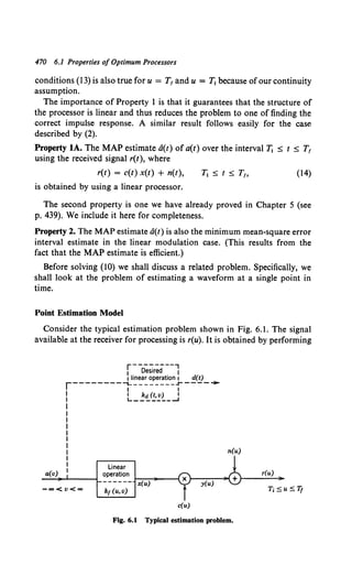
487. Gaussian Assumption 471
a linear operation on a(v) to obtain x(u), which is then multiplied by a
known modulation function. A noise n(u) is added to the output y(u)
before it is observed. The dotted lines represent some linear operation
(not necessarily time-invariant nor realizable) that we should like to
perform on a(v) if it were available (possibly for all time). The output is
the desired signal d(t) at some particular time t. The time t may or may not
be included in the observation interval.
Common examples of desired signals are:
(i) d(t) = a(t).
Here the output is simply the message. Clearly, if t were included in the
observation interval, x(u) = a(u), n(u) were zero, and c(u) were a constant,
we could obtain the signal exactly. In general, this will not be the case.
(ii) d(t) = a(t + a).
Here, if a is a positive quantity, we wish to predict the value of a(t) at
some time in the future. Now, even in the absence of noise the estimation
problem is nontrivial if t + a > T,. If a is a negative quantity, we shall
want the value at some previous time.
(iii)
d
d(t) = dt a(t).
Here the desired signal is the derivative of the message. Other types of
operations follow easily.
We shall assume that the linear operation is such that d(t) is defined in
the mean-square sense [i.e., if d(t) = d(t), as in (iii), we assume that a(t)
is a mean-square differentiable process]. Our discussion has been in the
context of the linear modulation system in Fig. 6.1. We have not yet
specified the statistics of the random processes. We describe the processes
by the following assumption:
Gaussian Assumption. The message a(t), the desired signal d(t), and the
received signal r(t) are jointly Gaussian processes.
This assumption includes the linear modulation problem that we have
discussed but avoids the necessity of describing the modulation system in
detail. For algebraic simplicity we assume that the processes are zero-mean.
We now return to the optimum processing problem. We want to operate
on r(u), T1 :0: u :0: T, to obtain an estimate ofd(t). We denote this estimate
as d(t) and choose our processor so that the quantity
(15)

488. 472 6.1 Properties of Optimum Processors
is minimized. First, observe that this is a point estimate (therefore the
subscript P). Second, we observe that we are minimizing the mean-square
error between the desired signal d(t) and the estimate d(t).
We shall now find the optimum processor. The approach is as follows:
1. First, we shall find the optimum linear processor. Properties 3, 4, 5,
and 6 deal with this problem. We shall see that the Gaussian assumption
is not used in the derivation of the optimum linear processor.
2. Next, by including the Gaussian assumption, Property 7 shows that
a linear processor is the best of all possible processors for the mean-square
error criterion.
3. Property 8 demonstrates that under the Gaussian assumption the
linear processor is optimum for a large class of error criteria.
4. Finally, Properties 9 and 10 show the relation between point
estimators and interval estimators.
Property 3. The minimum mean-square linear estimate is the output of a
linear processor whose impulse response is a solution to the integral
equation
(16)
The proof of this property is analogous to the derivation in Section
3.4.5. The output of a linear processor can be written as
fTf
d(t) = h(f, T) r(T) dT.
T,
(17)
We assume that h(t, T) = 0, T < T" T > T1 • The mean-square error at
time tis
fp(t) = {E[d(t) - J(t))2}
= E{[d<t)- I:.' h(t, T)r(T)dTf}- (18)
To minimize fp(t) we would go through the steps in Section 3.4.5 (pp.
198-204).
l. Let h(t, T) = h0 (t, T) + eh,(t, T).
2. Write fp(t) as the sum of the optimum error fp.(t) and an incremental
error ~f(t, e).
3. Show that a necessary and sufficient condition for ~f(t, e) to be
greater than zero for e =1- 0 is the equation
E{[d(t)- I:.' h0 (t,T)r(T)dT] r(u)} = 0, (19)

489. Property 3 473
Bringing the expectation inside the integral, we obtain
(20)
which is the desired result. In Property 7A we shall show that the solution
to (20) is unique iff Kr(t, u) is positive-definite.
We observe that the only quantities needed to design the optimum
linear processor for minimizing the mean-square error are the covariance
function of the received signal Kr(t, u) and the cross-covariance between
the desired signal and the received signal, Kar(t, u). We emphasize thafwe
have not used the Gaussian assumption.
Several special cases are important enough to be mentioned explicitly.
Property 3A. When d(t) = a(t) and T1 = t, we have a realizable filtering
problem, and (20) becomes
Kar(t. u) = Jt ho(t, T) Kr(T, u) dT,
Tt
T1 < u < t. (21)
We use the term realizable because the filter indicated by (21) operates
only on the past [i.e., h0 (t, T) = 0 forT > t].
Property 3B. Let r(t) = c(t) x(t) + n(t) £! y(t) + n(t). If the noise is
white with spectral height N0 /2 and uncorrelated with a(t), (20) becomes
Property 3C. When the assumptions of both 3A and 3B hold, and
x(t) = a(t), (20) becomes
No Jt
Ka(t, u) c(u) = 2 h0 (t, u) + h0 (t, T) c(T) Ka(T, u) c(u) dT,
Tt
T1 ~ u ~ t. (23)
[The end point equalities were discussed after (13).]
Returning to the general case, we want to find an expression for the
minimum mean-square error.
Property 4. The minimum mean-square error with the optimum linear
processor is
(24)

490. 474 6.1 Properties of Optimum Processors
This follows by using (16) in (18). Hereafter we suppress the subscript o
in the optimum error.
The error expressions for several special cases are also of interest. They
all follow by straightforward substitution.
Property 4A. When d(t) = a(t) and T1 = t, the minimum mean-square
error is
(25)
Property 4B. If the noise is white and uncorrelated with a(t), the error is
JT/
gp(t) = Ka(t, t) - h0 (t, T) Kay(t, T) dT.
Tt
(26)
Property 4C. If the conditions of 4A and 4B hold and x(t) = a(t), then
2
h0 (t, t) = No c(t) gp(t). (27)
If c- 1(t) exists, (27) can be rewritten as
gp(t) = ~0 c- 1(t) h0 (1, t). (28)
We may summarize the knowledge necessary to find the optimum
linear processor in the following property:
Property 5. Kr(t, u) and Kar(t, u) are the only quantities needed to find the
MMSE point estimate when the processing is restricted to being linear.
Any further statistical information about the processes cannot be used.
All processes, Gaussian or non-Gaussian, with the same Kr(t, u) and
Kar(t, u) lead to the same processor and the same mean-square error if the
processing is required to be linear.
Property 6. The error at time t using the optimum linear processor is
uncorrelated with the input r(u) at every point in the observation interval.
This property follows directly from (19) by observing that the first term
is the error using the optimum filter. Thus
E[e0 (t) r(u)] = 0, (29)
We should observe that (29) can also be obtained by a simple heuristic
geometric argument. In Fig. 6.2 we plot the desired signal d(t) as a point
in a vector space. The shaded plane area xrepresents those points that can
be achieved by a linear operation on the given input r(u). We want to

491. Property 7 475
Fig. 6.2 Geometric interpretation of the optimum linear filter.
choose d(t) as the point in x closest to d(t). Intuitively, it is clear that we
must choose the point directly under d(t). Therefore the error vector is
perpendicular to x (or, equivalently, every vector in x); that is,
e. (t) _L Jh(t, u) r(u) du for every h(t, u).
The only difficulty is that the various functions are random. A suitable
measure of the squared-magnitude of a vector is its mean-square value.
The squared magnitude of the vector representing the error is £[e2{t)].
Thus the condition of perpendicularity is expressed as an expectation:
E[e.(t) J:' h(t, u) r(u) du] = 0
for every continuous h(t, u); this implies
E[e.(t) r(u)] = 0,
which is (29) [and, equivalently, (19)].t
(30)
(31)
Property 6A. If the processes of concern d(t), r(t), and a(t) are jointly
Gaussian, the error using the optimum linear processor is statistically
independent of the input r(u) at every point in the observation interval.
This property follows directly from the fact that uncorrelated Gaussian
variables are statistically independent.
Property 7. When the Gaussian assumption holds, the optimum linear
processor for minimizing the mean-square error is the best of any type.
In other words, a nonlinear processor can not give an estimate with a
smaller mean-square error.
Proof Let d.(t) be an estimate generated by an arbitrary continuous
processor operating on r(u), T1 :::; u :::; T,. We can denote it by
d.(t) = f(t: r(u), Tt :::; u :::; T,). (32)
t Our discussion is obviously heuristic. It is easy to make it rigorous by introducing a
few properties of linear vector spaces, but this is not necessary for our purposes.

492. 476 6.1 Properties of Optimum Processors
Denote the mean-square error using this estimate as g.(t). We want to
show that
(33)
with equality holding when the arbitrary processor is the optimum linear
filter:
g.(t) = E{[d.(t) - d(t)]2}
= E{[d.(t) - d(t) + d(t) - d(t)]2}
= E{[d.(t) - d(t)]2} + 2E{[d.(t) - d(t)]e.(t)} + gp(t). (34)
The first term is nonnegative. It remains to show that the second term is
zero. Using (32) and (17), we can write the second term as
E{[f(t:r(u), T1 :;:; u :;:; T1)- I:.'h.(t, u) r(u) du]e.(t)} (35)
This term is zero because r(u) is statistically independent of e0 (t) over the
appropriate range, except for u = T1 and u = T1• (Because both processors
are continuous, the expectation is also zero at the end point.) Therefore
the optimum linear processor is as good as any other processor. The final
question of interest is the uniqueness. To prove uniqueness we must show
that the first term is strictly positive unless the two processors are equal.
We discuss this issue in two parts.
Property 7A. First assume thatf(t:r(u), T1 :;:; u :;:; T1) corresponds to a
linear processor that is not equal to h.(t, u). Thus
JTI
f(t:r(u), T1 :;:; u :;:; T1) = (h0(t, u) + h*(t, u)) r(u) du,
T,
(36)
where h.(t, u) represents the difference in the impulse responses.
Using (36) to evaluate the first term in (34), we have
Tt
E{[d.(t) - d(t)]2} = JJdu dz h*(t, u) K,(u, z) h.(t, z). (37)
T,
From (3.35) we know that if K,(u, z) is positive-definite the right-hand
side will be positive for every h.(t, u) that is not identically zero. On the
other hand, if K,(t, u) is only nonnegative definite, then from our dis-
cussion on p. 181 of Chapter 3 we know there exists an h.(t. u) such that
JTI
h.(t, u) K,(u, z) du = 0,
T,
(38)
Because the eigenfunctions of K,(u, z) do not form a complete orthonormal
set we can construct h.(t, u) out offunctions that are orthogonal to K,(u, z).

493. Property 8A 477
Note that our discussion in 7A has not used the Gaussian assumption
and that we have derived a necessary and sufficient condition for the
uniqueness of the solution of (20). If K,(u, z) is not positive-definite, we
can add an h.(t, u) satisfying (38) to any solution of (20) and still have a
solution. Observe that the estimate a(t) is unique even if K,(u, z) is not
positive-definite. This is because any h.(t, u) that we add to h0 (t, u) must
satisfy (38) and therefore cannot cause an output when the input is r(t).
Property 7B. Now assume that f(t:r(u), ]', :s; u :s; T1) is a continuous
nonlinear functional unequal to Jh0 (t, u) r(u) du. Thus
Tt
f(t:r(u), T, :S; u :S; T1) = Jh0 (t, u) r(u)du +J.(t:r(u), T1 :s; u :s; T1). (39)
Then
T,
E{[d.(t) - d(t)]2}
= E [f.(t:r(u), T1 :s; u :s; T1)J.(t:r(z), T1 :s; z :s; T1)]. (40)
Because r(u) is Gaussian and the higher moments factor, we can express
the expectation on the right in terms of combinations of K,(u, z). Carrying
out the tedious details gives the result that if K,(u, z) is positive-definite
the expectation will be positive unlessf.(t: r(z), ]', :s; z :s; T1)) is identically
zero.
Property 7 is obviously quite important. It enables us to achieve two
sets of results simultaneously by studying the linear processing problem.
I. If the Gaussian assumption holds, we are studying the best possible
processor.
2. Even if the Gaussian assumption does not hold (or we cannot justify
it), we shall have found the best possible linear processor.
In our discussion of waveform estimation we have considered only
minimum mean-square error and MAP estimates. The next property
generalizes the criterion.
Property 8A. Let e(t) denote the error in estimating d(t), using some
estimate d(t).
e(t) = d(t) - d(t). (41)
The error is weighted with some cost function C(e(t)). The risk is the
expected value of C(e(t)),
.1{(d(t), t) = E[C(e(t))] = E[C(d(t) - d(t))]. (42)
The Bayes point estimator is the estimate dit) which minimizes the
risk. If we assume that C(e(t)) is a symmetric convex upward function

494. 478 6.1 Properties ofOptimum Processors
and the Gaussian assumption holds, the Bayes estimator is equal to the
MMSE estimator.
JB(t) = J0 (t). (43)
Proof The proof consists of three observations.
1. Under the Gaussian assumption the MMSE point estimator at any
time (say t1) is the conditional mean of the a posteriori density
Pttc,lr<u>[Dt1 lr(u):Tl ;:S; u ;:S; T1]. Observe that we are talking about a single
random variable d11 so that this is a legitimate density. (See Problem 6.1.1.)
2. The a posteriori density is unimodal and symmetric about its con-
ditional mean.
3. Property 1 on p. 60 of Chapter 2 is therefore applicable and gives
the above conclusion.
Property 8B. If, in addition to the assumptions in Property 8A, we require
the cost function to be strictly convex, then
(44)
is the unique Bayes point estimator.
This result follows from (2.158) in the derivation in Chapter 2.
Property 8C. If we replace the convexity requirement on the cost function
with a requirement that it be a symmetric nondecreasing function such that
lim C(X)Ptt1 !r<u>[XJr(u): T1 ;:S; U :5 T,] = 0
x-oo 1
(45)
for all t1 and r(t) of interest, then (44) is still valid.
These properties are important because they guarantee that the proces-
sors we are studying in this chapter are optimum for a large class of
criteria when the Gaussian assumption holds.
Finally, we can relate our results with respect to point estimators and
MMSE and MAP interval estimators.
Property 9. A minimum mean-square error interval estimator is just a
collection of point estimators. Specifically, suppose we observe a waveform
r(u) over the interval T1 :5 u :5 T1 and want a signal d(t) over the interval
Ta :5 t :5 T8 such that the mean-square error averaged over the interval
is minimized.
~1 Q E{J:: [d(t) - d(t)]2 dt} (46)
Clearly, if we can minimize the expectation of the bracket for each t then
~1 will be minimized. This is precisely what a MMSE point estimator does.
Observe that the point estimator uses r(u) over the entire observation

495. Vector Properties 479
interval to generate d(t). (Note that Property 9 is true for nonlinear
modulation also.)
Property 10. Under the Gaussian assumption the minimum mean-square
error point estimate and MAP point estimate are identical. This is just a
special case of Property 8C. Because the MAP interval estimate is a
collection of MAP point estimates, the interval estimates also coincide.
These ten properties serve as background for our study of the linear
modulation case. Property 7 enables us to concentrate our efforts in this
chapter on the optimum linear processing problem. When the Gaussian
assumption holds, our results will correspond to the best possible pro-
cessor (for the class of criterion described above). For arbitrary processes
the results will correspond to the best linear processor.
We observe that all results carry over to the vector case with obvious
modifications. Some properties, however, are used in the sequel and
therefore we state them explicitly. A typical vector problem is shown in
Fig. 6.3.
The message a(t) is a p-dimensional vector. We operate on it with a
matrix linear filter which has p inputs and n outputs.
x(u) = J~, k1(u, v) a(v) dv,
.--------l
J k.i(t, v) I d(tJ
rr== = ==_,.,--Matr~fi~~;--- i==qxl~
:: L~i~~s.:_q~utp~J
II
II
II
II
II
II
II
II
II
II
n(u)
mx 1
y(u)
.:•=(=v)'==!!ii==~-- -~~~u~v2 ___ 1==x=(=u=)~
P x 1 Matrix filter n x 1 ..~ m x 1
"' ~(u)
)===:===( + m x 1
p inputs-n outputs
e(u)
mxn
Fig. 6.3 Vector estimation problem.
(47)

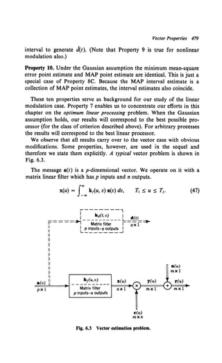
496. 480 6.1 Properties of Optimum Processors
The vector x(u) is multiplied by an m x n modulation matrix to give the
m-dimensional vector y(t) which is transmitted over the channel. Observe
that we have generated y(t) by a cascade of a linear operation with a
memory and no-memory operation. The reason for this two-step procedure
will become obvious later. The desired signal d(t) is a q x !-dimensional
vector which is related to a(v) by a matrix filter withp inputs and q outputs
Thus
d(t) = J:"" k4(t, v) a(v) dv. (48)
We shall encounter some typical vector problems later. Observ~ that p, q,
m, and n, the dimensions of the various vectors, may all be different.
The desired signal d(t) has q components. Denote the estimate of the
ith component as ~(t). We want to minimize simultaneously
i=l,2, ... ,q. (49)
The message a(v) is a zero-mean vector Gaussian process and the noise
is an m-dimensional Gaussian random process. In general, we assume that
it contains a white component w(t):
E[w(t) wT(u)] ~ R(t) S(t - u), (50)
where R(t) is positive-definite. We assume also that the necessary co-
variance functions are known. We shall use the same property numbers
as in the scalar case and add a V. We shall not restate the assumptions.
Property 3V.
K.sr(t, u) = IT' h0(t, T)Kr(T, u) dT,
T,
Proof See Problem 6.1.2.
Property 3A-V.
Kar(t, u) =It h0(t, T)Kr(T, u) dT;
T,
Property 4C-V.
(51)
T1 < u < t. (52)
h.(t, t) = ;p(t) CT(t) R -l(t), (53)
where ep(t) is the error covariance matrix whose elements are
gpil(t) ~ E{[a1(t) - a1(t)][a;(t) - a;(t)]}. (54)
(Because the errors are zero-mean, the correlation and covariance are
identical.)
Proof See Problem 6.1.3.
Other properties of the vector case follow by direct modification.

497. Summary 481
Summary
In this section we have explored properties that result when a linear
modulation restriction is imposed. Although we have discussed the
problem in the modulation context, it clearly has widespread applicability.
We observe that if we let c(t) = 1 at certain instants of time and zero
elsewhere, we will have the sampled observation model. This case and
others ofinterest are illustrated in the problems (see Problems 6.1.4-6.1.9).
Up to this point we have restricted neither the processes nor the observa-
tion interval. In other words, the processes were stationary or nonstation-
ary, the initial observation time T1 was arbitrary, and T1 ( ~ T1) Yas
arbitrary. Now we shall consider specific solution techniques. The easiest
approach is by means of various special cases.
Throughout the rest of the chapter we shall be dealing with linear
processors. In general, we do not specify explicitly that the Gaussian
assumption holds. It is important to re-emphasize that in the absence of
this assumption we are finding only the best linear processor (a nonlinear
processor might be better). Corresponding to each problem we discuss
there is another problem in which the processes are Gaussian, and for
which the processor is the optimum of all processors for the given criterion.
It is also worthwhile to observe that the remainder of the chapter could
have been studied directly after Chapter 1 if we had approached it as a
"structured" problem and not used the Gaussian assumption. We feel that
this places the emphasis incorrectly and that the linear processor should
be viewed as a device that is generating the conditional mean. This view-
point puts it into its proper place in the over-all statistical problem.
6.2 REALIZABLE LINEAR FILTERS: STATIONARY PROCESSES, INFINITE
PAST: WIENER FILTERS
In this section we discuss an important case relating to (20). First, we
assume that the final observation time corresponds to the time at which
the estimate is desired. Thus t = T1 and (20) becomes
Kdr(t, a) = It ho(t, u) Kr(U, a) du; T1 < a < t. (55)
Tt
Second, we assume that T1 = -oo. This assumption means that we have
the infinite past available to operate on to make our estimate. From a
practical standpoint it simply means that the past is available beyond the
significant memory time of our filter. In a later section, when we discuss
finite Tt. we shall make some quantitative statements about how large
t - Tt must be in order to be considered infinite.

498. 482 6.2 Wiener Filters
Third, we assume that the received signal is a sample function from a
stationary process and that the desired signal and the received signal are
jointly stationary. (In Fig. 6.1 we see that this implies that c(t) is constant.
Thus we say the process is unmodulated.t) Then we may write
Kdr(t - a) = f00
h0(t, u) Kr(u - a) du, -00 < a < t. (56)
Because the processes are stationary and the interval is infinite, let us try
to find a solution to (56) which is time-invariant.
Kdr(t - a) = f00
h0(t - u) Kr(u - a) du, -00 < a < t. (57)
If we can find a solution to (57), it will also be a solution to (56). If
Kr(u - a) is positive-definite, (56) has a unique solution. Thus, if (57) has
a solution, it will be unique and will also be the only solution to (56).
Letting T = t - a and v = t - u, we have
0 < T < 00, (58)
which is commonly referred to as the Wiener-Hopf equation. It was
derived and solved by Wiener [I]. (The linear processing problem was
studied independently by Kolmogoroff [2].)
6.2.1 Solution of Wiener-Hop( Equation
Our solution to the Wiener-Hopf equation is analogous to the approach
by Bode and Shannon [3]. Although the amount of manipulation required
is identical to that in Wiener's solution, the present procedure is more
intuitive. We restrict our attention to the case in which the Fourier trans-
form of Kr(T ), the input correlation function, is a rational function. This
is not really a practical restriction because most spectra of interest can be
approximated by a rational function. The general case is discussed by
Wiener [I] but does not lead to a practical solution technique.
The first step in our solution is to observe that if r(t) were white the
solution to (58) would be trivial. If
(59)
then (58) becomes
Kdr(T) = Loo h0 (v) 8(T - v) dv, 0 < T < 00, (60)
t Our use of the term modulatedis the opposite ofthe normal usage in which the message
process modulates a carrier. The adjective unmodulatedseems to be the best available.

499. Solution of Wiener-Hop/ Equation 483
r(t)
~a
z(t)
)
Fig. 6.4 Whitening filter.
and
ho(-r) = Kdr(-r), T <::: 0,
= 0, T < 0, (61)
where the value at -r = 0 comes from our continuity restriction.
It is unlikely that (59) will be satisfied in many problems of interest.
If, however, we could perform some preliminary operation on r(t) to
transform it into a white process, as shown in Fig. 6.4, the subsequent
filtering problem in terms of the whitened process would be trivial. The
idea of a whitening operation is familiar from Section 4.3 of Chapter 4.
In that case the signal was deterministic and we whitened only the noise.
In this case we whiten the entire input. In Section 4.3 we proved that any
reversible operation could not degrade the over-all system performance.
Now we also want the over-all processor to be a realizable linear filter.
Therefore we show the following property:
Whitening Property. For all rational spectra there exists a realizable,
time-invariant linear filter whose output z(t) is a white process when the
input is r(t) and whose inverse is a realizable linear filter.
If we denote the impulse response of the whitening filter as w(-r) and
the transfer function as WUw), then the property says:
(i) Is:"'w(u) w(v) K,(-r- u- v) du dv = 8(-r), -00 < T < 00.
or
(ii) IWUw)I2S,(w) = 1.
If we denote the impulse response of the inverse filter as w- 1(-r), then
(iii) J:"' w- 1(u - v) w(v) dv = S(u)
or
(iv)
and w- 1(-r) must be the impulse response of a realizable filter.
We derive this property by demonstrating a constructive technique for a
simple example and then extending it to arbitrary rational spectra.

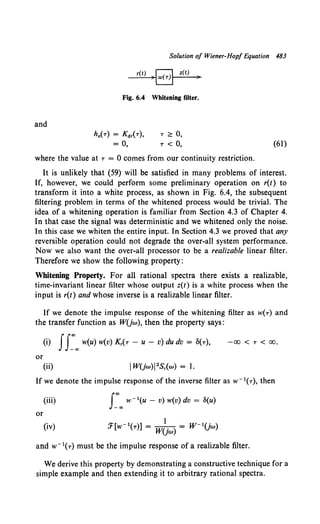
500. 484 6.2 Wiener Filters
Example I. Let
2k
S,(w) = w2 + k2. (62)
We want to choose the transfer function of the whitening filter so that it is realizable
and the spectrum of its output z(t) satisfies the equation
S.(w) = S,(w)l W(jw)J 2 = 1. (63)
To accomplish this we divide S,(w) into two parts,
( vzk)( vzk)
S,(w) = jw + k -jw + k !;:, [G•(jw)][G•(jw)]*. (64)
We denote the first term by G•(jw) because it is zero for negative time. The second
term is its complex conjugate. Clearly, if we let
. 1 jw + k
W(;w) = G•(jw) = V2k ' (65)
then (63) will be satisfied.
We observe that the whitening filter consists of a differentiator and a gain term in
parallel. Because
.y-
w-1(jw) = a•(jw) = ~.
JW + k
(66)
it is clear that the inverse is a realizable linear filter and therefore W(jw) is a legitimate
reversible operation. Thus we could operate on z(t) in either of the two ways shown
in Fig. 6.5 and, as we proved in Section 4.3, if we choose h~(T) in an optimum manner
the output of both systems will be d(t).
In this particular example the selection of W(jw) was obvious. We now
consider a more complicated example.
Example 2. Let
S( ) = c2(jw + a1)(-jw + rx,).
' "' (jw + {31)(- jw + {31)
H~ (jw)
Optimum operation
on z(t)
(a)
(b)
Fig. 6.5 Optimum filter: (a) approach No.1; (b) approach No.2.
(67)

501. Solution of Wiener-Hop! Equation 485
Assign
left-half
plane to
a+(s)
X
Assign
fSplit zeros on axis
. right-half
JW plane to
a+(-s)
X
s=u+jw
-------o--------~------<r------------~0'
X X
Fig. 6.6 A typical pole-zero plot.
We must choose W(jw) so that
(68)
and both W(jw) and w- 1(jw) [or equivalently G+(jw) and W(jw)] are realizable.
When discussing realizability, it is convenient to use the complex s-plane. We extend
our functions to the entire complex plane by replacing jw by s, where s = a + jw.
In order for W(s) to be realizable, it cannot have any poles in the right half of the
s-plane. Therefore we must assign the (jw + a1) term to it. Similarly, for w-1(s) [or
G+(s)] to be realizable we assign to it the (jw + {31) term. The assignment of the
constant is arbitrary because it adjusts only the white noise level. For simplicity we
assume a unity level spectrum for z(t) and divide the constant evenly. Therefore
G +(. ) _ (jw + al).
;w - c (jw + /31) (69)
To study the general case we consider the pole-zero plot of the typical
spectrum shown in Fig. 6.6. Assuming that this spectrum is typical, we
then find that the procedure is clear. We factor Sr(w) and assign all poles
and zeros in the left half plane (and half of each pair of zeros on the axis)
to G+(jw). The remaining poles and zeros will correspond exactly to the
conjugate [G+(jw)]*. The fact that every rational spectrum can be divided
in this manner follows directly from the fact that Sr(w) is a real, even,
nonnegative function of w whose inverse transform is a correlation
function. This implies the modes of behavior for the pole-zero plot shown
in Fig. 6.7a-c:

502. 486 6.2
X
X
Wiener Filters
jw
X
0 0
0 0
X
(a)
Symmetry about
(/'
u axis
--X
jw
Zeros on jw axis
in pairs
(poles can not be
on axis)
(c)
jw
(b)
0"
Fig. 6.7 Possible pole-zero plots in the s-plane.
Symmetry about
jw axis
I. Symmetry about the a-axis. Otherwise Sr(w) would not be real.
2. Symmetry about the jw-axis. Otherwise Sr(w) would not also be even.
3. Any zeros on the jw-axis occur in pairs. Otherwise Sr(w) would be
negative for some value of w.
4. No poles on thejw-axis. This would correspond to a l/w2 term whose
inverse is not the correlation function of a stationary process.
The verification of these properties is a straightforward exercise (see
Problem 6.2.1).
We have now proved that we can always find a realizable, reversible
whitening filter. The processing problem is now reduced to that shown in
Fig. 6.8. We must design H~Uw) so that it operates on z(t) in such a way
r(t)
Fig. 6.8 Optimum filter.

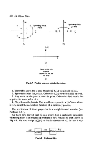
503. Solution of Wiener-Hop/ Equation 487
that it produces the minimum mean-square error estimate of d(t). Clearly,
then, h~(T) must satisfy (58) with r replaced by z,
Kdz(T) = {'" h~(v) Kz(T - v) dv, 0 < T < 00. (70)
However, we have forced z(t) to be white with unity spectral height.
Therefore
T 2!: 0. (71)
Thus, if we knew Ka2 ( T), our solution would be complete. Because z(t) is
obtained from r(t) by a linear operation, Ka2(r) is easy to find,
KazCT) ~ E[d(t) J~"' w(v) r(t- T- v) dv]
= f~"' w(v) KarCT + v) dv = f~"' w(- fJ) Kar(T - fJ) dfJ. (72)
Transforming,
S ( . ) W*(. ) S u· ) Sdr(jw)
dz }W = }W ar w = [G+(jw)]*' (73)
We simply find the inverse transform of Sa2Uw), Ka2 (r), and retain the
part corresponding to T 2!: 0. A typical Ka.(T) is shown in Fig. 6.9a. The
associated h~(r) is shown in Fig. 6.9b.
T
(a)
h~(T)
0 T
(b)
Fig. 6.9 Typical Functions: (a) a typical covariance function; (b) corresponding h~(T).

504. 488 6.2 Wiener Filters
We can denote the transform of KrJ2(r) for T ~ 0 by the symbol
[SrJ.z(jw)]+ Q f' KIJ.z(T)e-iw• dT = L"' h~(T)e-1"'' dT.t {74)
Similarly,
(75)
Clearly,
(76)
and we may write
H;(jw) = [S(}.zUw)]+ = [W*(jw) s(}.,(jw)]+ = [[;:~=~·L· (77)
Then the entire optimum filter is just a cascade of the whitening filter and
H;(jw),
H (. ) [ I ] [ S(}.,(jw) ]
0 JW = G+(jw) [G+(jw)]* +•
(78)
We see that by a series of routine, conceptually simple operations we have
derived the desired filter. We summarize the steps briefly.
l. We factor the input spectrum into two parts. One term, G+(s),
contains all the poles and zeros in the left half of the s-plane. The other
factor is its mirror image about the jw-axis.
2. The cross-spectrum between d(t) and z(t) can be expressed in terms
of the original cross-spectrum divided by[G+(jw)]*. This corresponds to a
function that is nonzero for both positive and negative time. The realizable
part of this function (T ~ 0) is h~(T) and its transform is H;(jw).
3. The transfer function of the optimum filter is a simple product of
these two transfer functions. We shall see that the composite transfer
function corresponds to a realizable system. Observe that we actually
build the optimum linear filter as single system. The division into two
parts is for conceptual purposes only.
Before we discuss the properties and implications of the solution, it
will be worthwhile to consider a simple example to guarantee that we all
agree on what (78) means.
Example 3. Assume that
r(t) = VP a(t) + n(t), (79)
t In general, the symbol [-1 + denotes the transform of the realizable part of the
inverse transform of the expression inside the bracket.

505. Solution of Wiener-Hop/ Equation 489
where a(t) and n(t) are uncorrelated zero-mean stationary processes and
2k
s.(w) = ~2 + k2. (80)
[We see that a(t) has unity power so that Pis the transmitted power.]
No
Sn(w) = T" (81)
The desired signal is
d(t) = a(t + a), (82)
where a is a constant.
By choosing a to be positive we have the prediction problem, choosing a to be zero
gives the conventional filtering problem, and choosing a to be negative gives the
filtering-with-delay problem.
The solution is a simple application of the procedure outlined in the preceding
section:
S( ) = ~ No= No w2 + k2 (l + 4P/kNo).
r w w2 + k2 + 2 2 w2 + k2
It is convenient to define
A= 4P.
kNo
(83)
(84)
(This quantity has a physical significance we shall discuss later. For the moment, it
can be regarded as a useful parameter.) First we factor the spectrum
(85)
so
G+(jw) = (N0 )Y.(jw +. kYT+A)· (86)
2 }W + k
Now
K.,(r) = E[d(t) r(t - r)] = E{a(t + a)[VP a(t - r) + n(t - r))}
= v:PE[a(t + a) a(t - r)] = ypK.(T + a). (87)
Transforming,
(88)
2kVPe+!wa (-jw + k)
w• + k2 vN0(2(-jw + kV1 +A).
(89)
To find the realizable part, we take the inverse transform:
K () _ :J<- 1{ s.,(jw) } _ :J<- 1 [ 2kv:Pe+!wa ]· (90)
dz T - [G+(jw)]* - (jw + k)VN0/2(-jw + kV1 +A)
The inverse transform can be evaluated easily (either by residues or a partial fraction
expansion and the shifting theorem). The result is
T +a~ 0,
(91)
r +a< 0.
The function is shown in Fig. 6.10.

506. 490 6.2 Wiener Filters
Fig. 6.10 Cross-covariance function.
Now h~(T) depends on the value a. In other words, the amount of K••(T) in the
range T ;;::: 0 is a function of a. We consider three types of operations:
Case 1. 11 = 0: filtering with zero delay. Letting a = 0 in (91), we have
or
Then
h.< ) 2v'"P 1 k• <>
• T = VNo/21 + VI +A e- U-1 T •
H'( 'w) = 1 2VP _1_.
•' l+Vl+AVN0 /2jw+k
(92)
(93)
Ho( 'w) = H;(jw) = 2v''P 1 . (94)
1 G+(jw) (No/2)(1 + ,;1 + A)jw + kVl +A
We see that our result is intuitively logical. The amplitude of the filter response is
shown in Fig. 6.11. The filter is a simple low-pass filter whose bandwidth varies as a
function of k and A.
We now want to attach some physical significance to the parameter A. The band-
width of the message process is directly proportional to k, as shown in Fig. 6.12a
log IIH.(jwJil
IHo(O)I
'iii'
1-lor-----------~r---~~~----------------~
~ ~w
-20
Fig. 6.11 Magnitude plot for optimum filter.

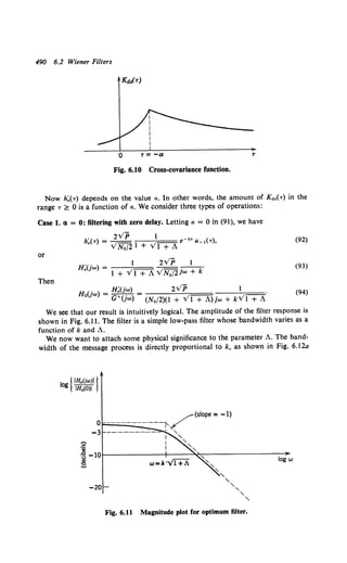
507. Solution of Wiener-Hop/ Equation 491
S~(w)
2/k 2/k
--'----L---'--~w/27r={
-k/4 +k/4
(a) (b)
Fig. 6.12 Equivalent rectangular spectrum.
The 3-db bandwidth is k/TT cps. Another common bandwidth measure is the equivalent
rectangular bandwidth (ERB), which is the bandwidth of a rectangular spectrum with
height S.(O) and the same total power of the actual message as shown in Fig. 6.12b.
Physically, A is the signal-to-noise ratio in the message ERB. This ratio is most
natural for most of our work. The relationship between A and the signal-to-noise
ratio in the 3-db bandwidth depends on the particular spectrum. For this particular
case Aadb = (TT/2)A.
We see that for a fixed k the optimum filter bandwidth increases as A, the signal-
to-noise ratio, increases. Thus, as A ...... oo, the filter magnitude approaches unity for
all frequencies and it passes the message component without distortion. Because the
noise is unimportant in this case, this is intuitively logical. On the other hand, as
A ...... 0, the filter 3-db point approaches k. The gain, however, approaches zero. Once
again, this is intuitively logical. There is so much noise that, based on the mean square
error criterion, the best filter output is zero (the mean value of the message).
Case 2. a is negative: filtering with delay. Here h~(r) has the impulse response shown
in Fig. 6.13. Transforming, we have
H;(jw) = 2kv'P [ e"1"'
VN0 /2 (jw + k)(-jw + kVl +A)
k(1 + v1 +-A;;::+ kV 1 + A)] (9S)
h~(T)
r= -a T
Fig. 6.13 Filtering with delay.

508. 492 6.2 Wiener Filters
This can be rewritten as
. 2kVP e"1"' [ _ (jw + k)e•<ko/f+A-iw>]·
H.(Jw) = (No/2)[w• + k•(I + A)] I k(l + vI + A) (96b)
We observe that the expression outside the bracket is just
s.,(jw) aiw
S,(w) e ·
(97)
We see that when a is a large negative number the second term in the bracket is
approximately zero. Thus H 0 (jw) approaches the expression in (97). This is just the
ratio of the cross spectrum to the total input spectrum, with a delay to make the
filter realizable.
We also observe that the impulse response in Fig. 6.13 is difficult to realize with
conventional network synthesis techniques.
Case 3. e1 is positive: filtering with prediction. Here
. ( 2VP 1 )
h.(-r) = VNo/21 +VI+ A e-k• e-ka, (98)
Comparing (98) with (92), we see that the optimum filter for prediction is just the
optimum filter for estimating a(t) multiplied by a gain e-k•, as shown in Fig. 6.14.
The reason for this is that a(r) is a first order wide-sense Markov process and the
noise is white. We obtain a similar result for more general processes in Section 6.3·
Before concluding our discussion we amplify a point that was en-
countered in Case 1 of the example. One step of the solution is to find the
realizable part of a function. Frequently it is unnecessary to find the time
function and then retransform. Specifically, whenever Sa,Uw) is a ratio of
two polynomials in jw, we may write
s:,(!w) * = F(jw) + i . C; + i .d; '
[G (Jw)] i= 1 jw + P1 ;=l -jw + q;
(99a)
where F(jw) is a polynomial, the first sum contains all terms corresponding
to poles in the left half of the s-plane (ir.cluding the jw-axis), and the
second sum contains all terms corresponding to poles in the right half of
Attenuator
Fig. 6.14 Filtering with prediction.

509. Errors in Optimum Systems 493
the s-plane. In this expanded form the realizable part consists of the first
two terms. Thus
[ Sdr(jw) ] F(. ) ~ C1
[G+(. )]* = }W + L ~+.·
}W + 1=1 }W p,
(99b)
The use of (99b) reduces the required manipulation.
In this section we have developed an algorithm for solving the Wiener-
Hopf equation and presented a simple example to demonstrate the
technique. Next we investigate the resulting mean-square error.
6.2.2 Errors in Optimum Systems
In order to evaluate the performance of the optimum linear filter we
calculate the minimum mean-square error. The minimum mean-square
error for the general case was given in (24) of Property 4. Because the
processes are stationary and the filter is time-invariant, the mean-square
error will not be a function of time. Thus (24) reduces to
gp = Ka(O)- f' ho(-r) Kar(r) dr.
Because ho(r) = 0 for r < 0, we can equally well write (100) as
gp = Ka(O) - J~00
h0 ( r) Kar(r) dr.
Now
where
K () _ ,._ 1 { Sdr(jw) } _ 1 Joo Sdr(jw) ;wtd
az t - :r [G+(jw)]* - 21r -oo [G+(jw)]* e w.
Substituting the inverse transform of (102) into (101), we obtain,
(100)
(101)
(102)
(103)
gP = Ka(O)- J~oo Kar(r) dr[2~ J~oo e1
w' dw· G+~jw) Loo Kaz(t)e-iwt dt].
(104)
Changing orders of integration, we have
gp = Kc~(O) - Loo Kc~z(t) dt [2~J~oo e-iwt dw G+~jw) J~oo Kar(r)eiwt dr].
(105)
The part of the integral inside the brackets is just KJ'.(t). Thus, since
Kc~.(t) is real,
(106)

510. 494 6.2 Wiener Filters
The result in (106) is a convenient expression for the mean-square error.
Observe that we must factor the input spectrum and perform an inverse
transform in order to evaluate it. (The same shortcuts discussed above are
applicable.)
We can use (106) to study the effect of a on the mean-square error.
Denote the desired signal when a = 0 as d0(t) and the desired signal for
arbitrary a as da(t) Q d0(t + a). Then
(107a)
and
E[d,.(t) z(t- T)] = E[d0(t +a) z(t- T)] = c/>(T +a). (107b)
We can now rewrite (106) in terms of c/>(T). Letting
Kdz(t) = c/>(t + a) (108a)
in (106), we have
Note that cf>(u) is not a function ofa. We observe that because the integrand
is a positive quantity the error is monotone increasing with increasing a.
Thus the smallest error is achieved when a = -oo (infinite delay) and
increases monotonely to unity as a~ +oo. This result says that for any
desired signal the minimum mean-square error will decrease if we allow
delay in the processing. The mean-square error for infinite delay provides
a lower bound on the mean-square error for any finite delay and is
frequently called the irreducible error. A more interesting quantity in
some cases is the normalized error. We define the normalized error as
or
We may now apply our results to the preceding example.
Example 3 (continued). For our example
~Pna = {
l _ SP } 2 (Jodt e+2k.l'i+At + J~ e-2kt dt),
No (l + V 1 + A) a a
1-SP l ("'e-•"'dt
No (1 + Vl + A)2 Ja '
(109a)
(109b)
a~ 0,
(llO)
a :2:: 0.

511. Errors in Optimum Systems 495
Evaluating the integrals, we have
aS 0, (111)
~Pno = 2 '
1 + v'1 +A
(112)
and
a~ 0. (113)
The two limiting cases for (Ill) and (113) are a= -cx:> and a= cx:>, respectively.·
~ _., 1
!OPn = V1 +A. (115)
(114)
A plot of ~Pna versus (ka) is shown in Fig. 6.15. Physically, the quantity ka is related
to the reciprocal of the message bandwidth. If we define
Tc = /(;' (116)
the units on the horizontal axis are a/T c• which corresponds to the delay measured in
correlation times. We see that the error for a delay of one time constant is approxi-
mately the infinite delay error. Note that the error is not a symmetric function of a.
Before summarizing our discussion of realizable filters, we discuss the
related problem of unrealizable filters.
~2~--~~---~.----0~.5~---o~--~~--~----~---.T(ka)
...,...._Filtering with delay 1 Prediction ~ -
Fig. 6.15 Elfect of time-shift on filtering error.

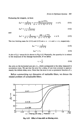
512. 496 6.2 Wiener Filters
6.2.3 Unrealizable Filters
Instead of requiring the processor to be realizable, let us consider an
optimum unrealizable system. This corresponds to letting T1 > t. In other
words, we use the input r(u) at times later than t to determine the estimate
at t.
For the case in which T1 > t we can modify (55) to obtain
Kdr(r) = f"' h0 (t, t-v) Kr(-r - v) dv, t - T1 < -r < oo. (117)
J!-Tt
In this case h0 (t, t-v) is nonzero for all v ~ t - T,. Because this includes
values of v less than zero, the filter will be unrealizable. The case of most
interest to us is the one in which T, = oo. Then (117) becomes
Kdr(-r) = J~.., hou(v)Kr(-r- v)dv, -00 < T < 00. (118)
We add the subscript u to emphasize that the filter is unrealizable. Because
the equation is valid for all -r, we may solve by transforming
H u )- sdT(jw).
ou w - Sr(w)
From Property 4, the mean-square error is
g,. = KiO) - I~.., hou(-r) Kdr(r) d-r.
(119)
(120)
Note that gu is a mean-square point estimation error. By Parseval's
Theorem,
gu = 2~ J~oo [Sd(w) - H0 u(jw) SJ'r(jw)] dw. (121)
Substituting (119) into (121), we obtain
(122)
For the special case in which
d(t) = a(t),
r(t) = a(t) + n(t),
(123)
and the message and noise are uncorrelated, (122) reduces to
(124)

513. Unrealizable Filters 497
In the example considered on p. 488, the noise is white. Therefore,
H (. ) = VP Sa(w)
ou }W Sr(w) ' (125)
and
g = No Joo H Uw) dw = No Joo VP Sa(w) dw. (l26)
u 2 _00 ou 27T 2 -oo Sr(w) 27T
We now return to the general case. It is easy to demonstrate that the
expression in (121) is also equal to
gu = K11(0) - s:oo I/J2(t) dt. (127)
Comparing (127) with (107) we see that the effect of using an unrealizable
filter is the same as allowing an infinite delay in the desired signal. This
result is intuitively logical. In an unrealizable filter we allow ourselves
(fictitiously, of course) to use the entire past and future of the input and
produce the desired signal at the present time. A practical way to approxi-
mate this processing is to wait until more of the future input comes in and
produce the desired output at a later time. In many, if not most,communi-
cations problems it is the unrealizable error that is a fundamental system
limitation.
The essential points to remember when discussing unrealizable filters
are the following:
1. The mean-square error using an unrealizable linear filter (T1 = oo)
provides a lower bound on the mean-square error for any realizable linear
filter. It corresponds to the irreducible (or infinite delay) error that we
encountered on p. 494. The computation of gu (124) is usually easier than
the computation of gp (100) or (106). Therefore it is a logical preliminary
calculation even if we are interested only in the realizable filtering problem.
2. We can build a realizable filter whose performance approaches the
performance of the unrealizable filter by allowing delay in the output. We
can obtain a mean-square error that is arbitrarily close to the irreducible
error by increasing this delay. From the practical standpoint a delay of
several times the reciprocal of the effective bandwidth of [Sa(w) + Sn(w)]
will usually result in a mean-square error close to the irreducible error.
We now return to the realizable filtering problem. In Sections 6.2.1 and
6.2.2 we devised an algorithm that gave us a constructive method for
finding the optimum realizable filter and the resulting mean-square error.
In other words, given the necessary information, we can always (con-
ceptually, at least) proceed through a specified procedure and obtain the
optimum filter and resulting performance. In practice, however, the

514. 498 6.2 Wiener Filters
algebraic complexity has caused most engineers studying optimum filters
to use the one-pole spectrum as the canonic message spectrum. The lack
of a closed-form mean-square error expression which did not require a
spectrum factorization made it essentially impossible to study the effects
of different message spectra.
In the next section we discuss a special class of linear estimation
problems and develop a closed-form expression for the minimum mean-
square error.
6.2.4 Closed-Form Error Expressions
In this section we shall derive some useful closed-form results for a
special class of optimum linear filtering problems. The case of interest is
when
r(u) = a(u) + n(u), -00 < u ::;; t. (128)
In other words, the received signal consists of the message plus additive
noise. The desired signal d(t) is the message a(t). We assume that the
noise and message are uncorrelated. The message spectrum is rational with
a finite variance. Our goal is to find an expression for the error that does
not require spectrum factorization. The major results in this section were
obtained originally by Yovits and Jackson (4]. It is convenient to consider
white and nonwhite noise separately.
Errors in the Presence of White Noise. We assume that n(t) is white
with spectral height N0/2. Although the result was first obtained by Yovits
and Jackson, appreciably simpler proofs have been given by Viterbi and
Cahn [5], Snyder[6], and Helstrom [57]. We follow a combination of these
proofs. From (128)
(129)
and
G+(jw) = [ Sa(jw) + ~o] + · (130)
From (78)
(l3l)t
tTo avoid a double superscript we introduce the notation
G-(jw) = [G+(jw))*.
Recall that conjugation in the frequency domain corresponds to reversal in the time
domain. The time function corresponding to G+(jw) is zero for negative time.
Therefore the time function corresponding to c-(jw) is zero for positive time.

515. Closed-Form Error Expressions 499
or
HUw _ 1 { Sa(w) + N0/2 _ N0 f2 } .
0 ) - [Sa(w) + No/2]+ [Sa(w) + No/2]- [Sa(w) + No/2]- +
(132)
Now, the first term in the bracket is just [Sa(w) + N0/2] +, which is
realizable. Because the realizable part operator is linear, the first term
comes out of the bracket without modification. Therefore
(' ) 1 { N0 /2 }
Ho jw = l - [Sa(w) + No/2]+ [Sa(w) + No/2] / (133)
We take VN0/2 out of the brace and put the remaining VN0/2 inside the
[·]-. The operation [·]- is a factoring operation so we obtain N0 /2 inside.
. v'N;fi { 1 }
HaUw) = l - [Sa(w) + No/2]+ [Sa(w) + No/2] (l 34)
N0/2 +
The next step is to prove that the realizable part of the term in the brace
equals one.
Proof Let Sa(w) be a rational spectrum. Thus
N(w2)
Sa(w) = D(w2)' (135)
where the denominator is a polynomial in w 2 whose order is at least one
higher than the numerator polynomial. Then
N(w2) + (N0/2) D(w2)
(N0 /2) D(w2)
D(w2) + (2/N0) N(w2)
D(w2)
(136)
(137)
(138)
Observe that there is no additional multiplier because the highest order
term in the numerator and denominator are identical.
The a1 and {31 may always be chosen so that their real parts are positive.
If any of the a1 or {31 are complex, the conjugate is also present. Inverting
both sides of (138) and factoring the result, we have
{[Sa(w) + N0/2] -}-1
= rl(-!w + f3t) (139)
N0/2 1= 1 ( -jw + a 1)
= fJ [l + (!;w-+a~iJ (140)

516. 500 6.2 Wiener Filters
The transform of all terms in the product except the unity term will be
zero for positive time (their poles are in the right-halfs-plane). Multiplying
the terms together corresponds to convolving their transforms. Convolving
functions which are zero for positive time always gives functions that are
zero for positive time. Therefore only the unity term remains when we take
the realizable part of (140). This is the desired result. Therefore
(141)
The next step is to derive an expression for the error. From Property 4C
(27-28) we know that
t. - No I' h ( ) - No I' h ( ) t:o Noh (O+
SP - 2 ,~I[! o f, T - 2 ,!.r:!+ oE - 2 o ) (142)
for the time-invariant case. We also know that
fro Ho(jw) dw = h0 (0+) + h0 (0-) = ho(Q+), 043)
-co 27T 2 2
because h0(T) is realizable. Combining (142) and (143), we obtain
~P = No J~co Ho(jw) ~:· (144)
Using (141) in (144), we have
gp = No Jco (t _{[Sa(w) + No/2] +}-1
) dw. 045)
-co N0/2 27T
Using the conjugate of (139) in (145), we obtain
~P = No Jco [1 - fr (!w + /3;)] dw, (146)
- co ;~ 1 (jw + a;) 27T
~P = No J"' [1 - TI (1 + ~; -a;)] dw. (147)
_ "' i ~ 1 ;w + a; 27T
Expanding the product, we have
"~ " " Yt;
J
co { [ n a n n
gP =No -oo l - l + i~jw +a;+ i~ i~1 (jw + a;)(jw +a;)
(148)
-No L L . Yii_ + L L L ... ~- (149)
J"' [n n n n n Jd
-co t~1 1~1 (Jw + a;)(jw +a;) t~1 1~1 k~1 27T

517. Closed-Form Error Expressions 501
The integral in the first term is just one half the sum of the residues
(this result can be verified easily). We now show that the second term is
zero. Because the integrand in the second term is analytic in the right half
of the s-plane, the integral [-oo, oo] equals the integral around a semicircle
with infinite radius. All terms in the brackets, however, are at least of
order lsi- 2 for large lsi. Therefore the integral on the semicircle is zero,
which implies that the second term is zero. Therefore
No n
~P = 2 L (a; - {3;).
t= 1
(I 50)
The last step is to find a closed-form expression for the sum of the
residues. This follows by observing that
(To verify this equation integrate the left-hand
u = In [(w2 + a;2)/(w2 + {3;2)] and dv = dwj2TT.)
Comparing (150), (151), and (138), we have
1:. _ N 0 I"' l [t Sa(w)] dw
~P-- n + -- -,
2 - oo N0 /2 2TT
(151)
side by parts with
(!52)
which is the desired result. Both forms of the error expressions (150) and
(152) are useful. The first form is often the most convenient way to actually
evaluate the error. The second form is useful when we want to find the
Sa(w) that minimizes ep subject to certain constraints.
It is worthwhile to emphasize the importance of (152). In conventional
Wiener theory to investigate the effect of various message spectra we had
to actually factor the input spectrum. The result in (152) enables us to
explore the error behavior directly. In later chapters we shall find it
essential to the solution for the optimum pre-emphasis problem in angle
modulation and other similar problems.
We observe in passing that the integral on the right-hand side is equal to
twice the average mutual information (as defined by Shannon) between
r(t) and a(t).
Errors for Typical Message Spectra. In this section we consider two
families of message spectra. For each family we use (152) to compute the
error when the optimum realizable filter is used. To evaluate the improve-
ment obtained by allowing delay we also use (124) to calculate the un-
realizable error.

518. 502 6.2 Wiener Filters
Case 1. Butterworth Family. The message processes in the first class have
spectral densities that are inverse Butterworth polynomials of order 2n.
From (3.98),
. _ 2nP sin (7r/2n) 1:::, en •
Sa(w.n) - k l + (w/k)2n- 1 + (w/k)2n (153)
The numerator is just a gain adjusted so that the power in the message
spectrum is P.
Some members of the family are shown in Fig. 6.16. For n = I we have
the one-pole spectrum ofSection 6.2.1. The break-point is at w = k rad/sec
and the magnitude decreases at 6 db/octave above this point. For higher n
the break-point remains the same, but the magnitude decreases at 6n db/
octave. For n = oo we have a rectangular bandlimited spectrum
lO.Or---------,.-------,-------.-------,
2001----------
loO
i
?I Oo01
00 oil!
~~
rJ1
1o-~0Lol
_________o~ol~--------~L7o-~-L--~;~---~--_j
(T)-
Fig. 6.16 Butterworth spectra.

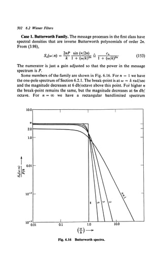
519. Closed-Form Error Expressions 503
[height P1r{k; width k radfsec]. We observe that if we use k/1r cps as the
reference bandwidth (double-sided) the signal-to-noise ratio will not be a
function of n and will provide a useful reference:
As!:::. p = 21TP.
- k/1r ·N0 /2 kNo
(154)
To find eP we use (152):
t: N0 Joo dw I [ 2c,.{N0 ]
~>P = T _oo 27T n 1 + 1 + (wfk)2" •
(155)
This can be integrated (see Problem 6.2.18) to give the following expression
for the normalized error:
ep,. = ;s(sin ;,) - 1
[ ( 1 + 2n ~s sin ;,)112
" - 1]. (156)
Similarly, to find the unrealizable error we use (124):
Joo dw C
eu = _ oo 21r 1 + (w/k)2" (2/No)c,.·
(157)
This can be integrated (see Problem 6.2.19) to give
[
2n 1T ] <1t2n>- 1
eu.. = 1 + -:;; As sin 2n · (158)
The reciprocal of the normalized error is plotted versus As in Fig. 6.17.
We observe the vast difference in the error behavior as a function ofn. The
most difficult spectrum to filter is the one-pole spectrum. We see that
asymptotically it behaves linearly whereas the bandlimited spectrum
behaves exponentially. We also see that for n = 3 or 4 the performance is
reasonably close to the bandlimited (n = oo) case. Thus the one-pole
message spectrum, which is commonly used as an example, has the worst
error performance.
A second observation is the difference in improvement obtained by use
of an unrealizable filter. For the one-pole spectrum
(n = 1). (159)
In other words, the maximum possible ratio is 2 (or 3 db). At the other
extreme for n = oo
(160)
whereas
(161)

520. Fig. 6.17 Reciprocal of mean-square error, Butterworth spectra:
504 (a) realizable; (b) unrealizable

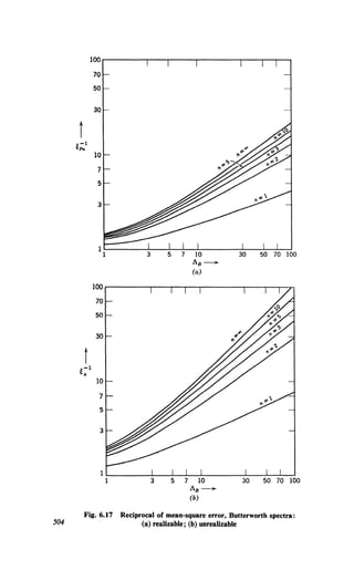
521. Closed-Form Error Expressions 505
Thus the ratio is
eun Js 1
ePn = I + JB In (I + Js).
(162)
For n = oo we achieve appreciable improvement for large J8 by allowing
delay.
Case 2. Gaussian Family. A second family of spectra is given by
S . ) _ 2Py; r(n) 1 t::,. dn
a(w.n - kvn r(n- !) (I + w2fnP)n- (l + w2fnP)n'
(163)
obtained by passing white noise through n isolated one-pole filters. In. the
limit as n ~ oo, we have a Gaussian spectrum
I. < ) 2v; 2[k2
1m Sa w:n = -k Pe-"' .
n-ao
(164)
The family of Gaussian spectra is shown in Fig. 6.18. Observe that for
n = I the two cases are the same.
The expressions for the two errors of interest are
(165)
and
l Jao dw dn
gun= p -ao 27T (I + w2jnk2)n + (2/No)dn.
(166)
To evaluate gPn we rewrite (165) in the form of (150). For this case the
evaluation of a 1 and {31 is straightforward [53]. The results for n = 1,2,3,
and 5 are shown in Fig. 6.I9a. For n = oo the most practical approach is
to perform the integration numerically. We evaluate (166) by using a
partial fraction expansion. Because we have already found the a1 and P~o
the residues follow easily. The results for n = 1, 2, 3, and 5 are shown in
Fig. 6.l9b. For n = oo the result is obtained numerically. By comparing
Figs. 6.17 and Fig. 6.19 we see that the Gaussian spectrum is more difficult
to filter than the bandlimited spectrum. Notice that the limiting spectra in
both families were nonrational (they were also not factorable).
In this section we have applied some of the closed-form results for the
special case of filtering in the presence of additive white noise. We now
briefly consider some other related problems.
Colored Noise and Linear Operations. The advantage of the error
expression in (152) was its simplicity. As we proceed to more complex
noise spectra, the results become more complicated. In almost all cases
the error expressions are easier to evaluate than the expression obtained
from the conventional Wiener approach.

522. 506 6.2 Wiener Filters
10.0
2 -.fif
2.0
1.0
i
0.3
?I 0.1
3 of!!
'-ii::
rJ]
(!f)-
Fig. 6.18 Gaussian family.
For our purposes it is adequate to list a number of cases for which
answers have been obtained. The derivations for some of the results are
contained in the problems (see Problems 6.2.20 to 6.2.26).
l. The message a(t) is transmitted. The additive noise has a spectrum
that contains poles but not zeros.
2. The message a(t) is passed through a linear operation whose transfer
function contains only zeros before transmission. The additive noise is
white.
3. The message a(t) is transmitted. The noise has a polynomial spectrum
Sn(w) = No + N2w2 + N4w4 + ···+ N2 nw2n.
4. The message a(t) is passed through a linear operation whose transfer
function contains poles only. The noise is white.

523. 5 7 10 20 30
As-
(a.)
Fig. 6.19 Reciprocal of mean-square error: Gaussian family,
(a) realizable; (b) unrealizable. 507

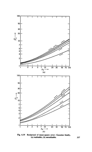
524. 508 6.2 Wiener Filters
We observe that Cases 2 and 4 will lead to the same error expression as
Cases 1 and 3, respectively.
To give an indication ofthe form ofthe answer we quote the result for
typical problems from Cases 1 and 4.
Example (from Case 1). Let the additive noise n(t} be uncorre1ated with the message
and have a spectrum,
(167)
Then
eP = an2
exp (- a~• roo Sn(w} In [1 + ~:~:n ~:)· (168)
This result is derived in Problem 6.2.20.
Example (from Case 4). The message a(t) is integrated before being transmitted.
r(t) = f oo a(u) du + w(t). (169)
Then
(170)
where
I _ foo I [1 2Sa(w}] dw
~- n +---•
- oo w 2 No 21T
(171)
12 = N0 foo w• In [I + 2S;(w}] dw.
2 -oo wNo 21T
(172)
This result is derived in Problem 6.2.25.
It is worthwhile to point out that the form of the error expression
depends only on the form of the noise spectrum or the linear operation.
This allows us to vary the message spectrum and study the effects in an
easy fashion.
As a final topic in our discussion of Wiener filtering, we consider
optimum feedback systems.
6.2.5 Optimum Feedback Systems
One of the forms in which optimum linear filters are encountered in the
sequel is as components in a feedback system. The modification of our
results to include this case is straightforward.
We presume that the assumptions outlined at the beginning of Section
6.2 (pp. 481-482) are valid. In addition, we require the linear processor to
have the form shown in Fig. 6.20. Here g1(r) is a linear filter. We are
allowed to choose g1(r) to obtain the best d(t).
System constraints of this kind develop naturally in the control system
context (see [9]). In Chapter 11.2 we shall see how they arise as linearized

525. Optimum Feedback Systems 509
r-----------------l
I I
I I
r(t) I 1d(t)
I + I
I I
I I
I I
I I
I I
L _________________ j
Overall filter
Fig. 6.20 Feedback system.
versions of demodulators. Clearly, we want the closed loop transfer
function to equal H0 Uw). We denote the loop filter that accomplishes this
as G10Uw). Now,
HU) = GzoUw)
o w 1 + GzoUw)
(173)
Solving for G10Uw),
(174)
For the general case we evaluate H0 Uw) by using (78) and substitute
the result into (174).
For the special case in Section 6.2.4, we may write the answer directly.
Substituting (141) into (174), we have
(175)
We observe that G10Uw) has the same poles as G+Uw) and is therefore a
stable, realizable filter. We also observe that the poles of G+Uw) (and
therefore the loop filter) are just the left-half-s-plane poles of the message
spectrum.
We observe that the message can be visualized as the output of a linear
filter when the input is white noise. The general rational case is shown in
Fig. 6.2la. We control the power by adjusting the spectral height of u(t):
E[u(t) u(T)] ~ q 8(t - T). (176)
The message spectrum is
(177)

526. 510 6.2 Wiener Filters
bn-1 sn-1 +••• +bo
u(t) ~ 1---~ a(t)
+
r(t)--;>o(
sn + Pn-1 sn-1 + ••• +Po
(a)
fn -1 sn-1 + ••• +~0
_...:.:_~-----;----
11 - ~---.-~fi(t)
sn + Pn-1 sn-1 + ••• +Po
(b)
Fig. 6.21 Filters: (a) message generation; (b) canonic feedback filter.
The numerator must be at least one degree less than the denominator to
satisfy the finite power assumption in Section 6.2.4. From (175) we see
that the optimum loop filter has the same poles as the filter that could be
used to generate the message. Therefore the loop filter has the form shown
in Fig. 6.2lb. It is straightforward to verify that the numerator of the loop
filter is exactly one degree less than the denominator (see Problem 6.2.27).
We refer to the structure in Fig. 6.2lb as the canonic feedback realization
of the optimum filter for rational message spectra [21 ]. In Section 6.3 we
shall find that a general canonic feedback realization can be derived by for
nonstationary processes and finite observation intervals.
Observe that to find the numerator we must still perform a factoring
operation (see Problem 6.2.27). We can also show that the first coefficient
in the numerator is 2~pjN0 (see Problem 6.2.28).
A final question about feedback realizations of optimum linear filters
concerns unrealizable filters. Because we have seen in Sections 6.2.2 and
6.2.3 [(108b) and (127)] that using an unrealizable filter (or allowing delay)
always improves the performance, we should like to make provision for it
in the feedback configuration. Previously we approximated unrealizable
filters by allowing delay. Looking at Fig. 6.20, we see that this would not
work in the case of g1
(T) because its output is fed back in real time to
become part of its input.
If we are willing to allow a postloop filter, as shown in Fig. 6.22, we
can consider unrealizable operations. There is no difficulty with delay in
the postloop filter because its output is not used in any other part of the
system.

527. Comments 511
r(t) +
Fig. 6.22 Unrealizable postloop filter.
The expression for the optimum unrealizable postloop filter GpuoCJw)
follows easily. Because the cascade of the two systems must correspond to
HauUw) and the closed loop to H0 (jw), it follows that
G U ) = Hou(jw).
puo W Ha(jw) (178)
The resulting transfer function can be approximated arbitrarily closely by
allowing delay.
6.2.6 Comments
In this section we discuss briefly some aspects of linear processing that
are of interest and summarize our results.
Related Topics. Multidimensional Problem. Although we formulated the
vector problem in Section 6.1, we have considered only the solution
technique for the scalar problem. For the unrealizable case the extension
to the vector problem is trivial. For the realizable case in which the
message or the desired signal is a vector and the received waveform is a
scalar the solution technique is an obvious modification of the scalar
technique. For the realizable case in which the received signal is a vector,
the technique becomes quite complex. Wiener outlined a solution in [I]
which is quite tedious. In an alternate approach we factor the input spectral
matrix. Techniques are discussed in [10] through [19].
Nonrational Spectra. We have confined our discussion to rational
spectra. For nonrational spectra we indicated that we could use a rational
approximation. A direct factorization is not always possible.
We can show that a necessary and sufficient condition for factorability
is that the integral
J"' 'log Sr(w) Id
_"' l + (w/27T)2 w

528. 512 6.2 Wiener Filters
must converge. Here S,(w) is the spectral density of the entire received
waveform. This condition is derived and the implications are discussed
in [I]. It is referred to as the Paley- Wiener criterion.
If this condition is not satisfied, r(t) is termed a deterministic waveform.
The adjective deterministic is used because we can predict the future of
r(t) exactly by using a linear operation on only the past data. A simple
example of a deterministic waveform is given in Problem 6.2.39.
Both limiting message spectra in the examples in Section 6.2.4 were
deterministic. This means, if the noise were zero, we would be able to
predict the future of the message exactly. We can study this beha~ior easily
by choosing some arbitrary prediction time a and looking at the prediction
error as the index n ~ oo. For an arbitrary a we can make the mean-square
prediction error less than any positive number by letting n become
sufficiently large (see Problem 6.2.41).
In almost all cases the spectra of interest to us will correspond to non-
deterministic waveforms. In particular, inclusion of white noise in r(t)
guarantees factorability.
Sensitivity. In the detection and parameter estimation areas we discussed
the importance of investigating how sensitive the performance of the
optimum system was with respect to the detailed assumptions of the model.
Obviously, sensitivity is also important in linear modulation. In any
particular case the technique for investigating the sensitivity is straight-
forward. Several interesting cases are discussed in the problems (6.2.31-
6.2.33).
In the scalar case most problems are insensitive to the detailed assump-
tions. In the vector case we must exercise more care.
As before, a general statement is not too useful. The important point to
re-emphasize is that we must always check the sensitivity.
Colored and White Noise. When trying to estimate the message a(t) in
the presence of noise containing both white and colored components, there
is an interesting interpretation of the optimum filter.
Let
and
r(t) = a(t) + nc(t) + w(t),
d(t) = a(t).
(179)
(180)
Now, it is clear that if we knew nc(t) the optimum processor would be
that shown in Fig. 6.23a. Here h0(T) is just the optimum filter for r'(t)
=a(t) + w(t), which we have found before.
We do not know nc(t) because it is a sample function from a random
process. A logical approach would be to estimate nc(t), subtract the
estimate from r(t), and pass the result through h0( T ), as shown in Fig. 6.23b.

529. Linear Operations and Filters 513
r(t) +
(a)
r(t)
(b)
Fig. 6.23 Noise estimation.
We can show that the optimum system does exactly this (see Problem
6.2.34). (Note that o(t) and nc(t) are coupled.) This is the same kind of
intuitively pleasing result that we encountered in the detection theory area.
The optimum processor does exactly what we would do if the disturbances
were known exactly, only it uses estimates.
Linear Operations and Filters. In Fig. 6.1 we showed a typical estimation
problem. With the assumptions in this section, it reduces to the problem
shown in Fig. 6.24. The general results in (78), (119), and (122) are applic-
able. Because most interesting problems fall into the model in Fig. 6.24,
it is worthwhile to state our results in a form that exhibits the effects of
ka(T) and k1( T) explicitly. The desired relations for uncorrelated message
and noise are
r---~--~~
I
t
I n(u)
a(~~~)~l~--~)~~x~~~~--~)~~r~~~~--~
Fig. 6.24 Typical unmodulated estimation problem.
(181)

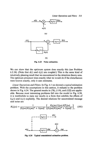
530. 514 6.2 Wiener Filters
and
H (j ) = Ka(jw) Sa(w) Kr*(jw) .
ou w Sa(w)JK1(jw)J 2 + Sn(w)
(182)
In the realizable filtering case we must use (181) whenever d(t) # a(t).
By a simple counterexample (Problem 6.2.38) we can show that linear
filtering and optimum realizable estimators do not commute in general.
In other words, d(t) does not necessarily equal
This result is in contrast to that obtained for MAP interval estimators.
On the other hand, comparing (119) with (182), we see that linear filtering
and optimum unrealizable (T1 = oo) estimators do commute. The resulting
error in the unrealizable case when KaUw) = I is
g = J"" Sa(w) Sn(w) dw.
uo -co Sa(w)JK1(jw)IZ + Sn(w) h
(183)
This expression is obvious. For other Kd(jw) see Problem 6.2.35. Some
implications of (183) with respect to the prefiltering problem are discussed
in Problem 6.2.36.
Remember that we assumed that ka(T) represents an "allowable"
operation in the mean-square sense; for example, if the desired operation
is a differentiation, we assume that a(t) is a mean-square differentiable
process (see Problem 6.2.37 for an example of possible difficulties when
this assumption is not true).
Summary. We have discussed in some detail the problem of linear
processing for stationary processes when the infinite past was available.
The principal results are the following:
1. A constructive solution to the problem is given in (78):
Ho(jw) = a+~jw) [[g:<Y=~*] +.
(78)
2. The effect of delay or prediction on the resulting error in an
optimum linear processor is given in (108b). In all cases there is a monotone
improvement as more delay is allowed. In many cases the improvement is
sufficient to justify the resulting complexity.
3. The importance of the idea that an unrealizable filter can be approxi-
mated arbitrarily closely by allowing a processing delay. The advantage of
the unrealizable concept is that the answer can almost always be easily
obtained and represents a lower bound on the MMSE in any system.

531. Summary 515
4. A closed-form expression for the error in the presence of white noise
is given in (152),
i: _ No Joo l [l Sa{w)] dw
~P-- n + -- -·
2 - oo N0 /2 27T
(152)
5. The canonic filter structure for white noise shown in Fig. 6.21 enables
us to relate the complexity of the optimum filter to the complexity of the
message spectra by inspection.
We now consider another approach to the point estimation problem.
6.3 KALMAN-BUCY FILTERS
Once again the basic problem of interest is to operate on a received
waveform r(u), T1 ~ u ~ t, to obtain a minimum mean-square error point
estimate of some desired waveform d(t). In a simple scalar case the
received waveform is
r(u) = c(u) a(u) + n(u), (184)
where a(t) and n(t) are zero-mean random processes with covariance
functions Ka(t, u) and (N0/2) 8(t - u), respectively, and d(t) = a(t). The
problem is much more general than this example, but the above case is
adequate for motivation purposes.
The optimum processor consists of a linear filter that satisfies the
equation
T1 < a< t. (185)
In Section 6.2 we discussed a special case in which T1 = - oo and the
processes were stationary. As part of the solution procedure we found a
function G+(jw). We observed that if we passed white noise through a
linear system whose transfer function was G+(jw) the output process had
a spectrum Sr(w). We also observed that in the white noise case, the filter
could be realized in what we termed the canonic feedback filter form. The
optimum loop filter had the same poles as the linear system whose output
spectrum would equal Sa(w) if the input were white noise. The only
problem was to find the zeros of the optimum loop filter.
For the finite interval it is necessary to solve (185). In Chapter 4 we dealt
with similar equations and observed that the conversion of the integral
equation to a differential equation with a set of boundary conditions is a
useful procedure.

532. 516 6.3 Kalman-Bucy Filters
We also observed in several examples that when the message is a
scalar Markov process [recall that for a stationary Gaussian process this
implies that the covariance had the form A exp (-Bit- ul)] the results
were simpler. These observations (plus a great deal of hindsight) lead us to
make the following conjectures about an alternate approach to the problem
that might be fruitful:
I. Instead of describing the processes of interest in terms of their
covariance functions, characterize them in terms of the linear (possibly
time-varying) systems that would generate them when driven with white
noise.t
2. Instead of describing the linear system that generates the message in
terms of a time-varying impulse response, describe it in terms of a differen-
tial equation whose solution is the message. The most convenient descrip-
tion will turn out to be a first-order vector differential equation.
3. Instead of specifying the optimum estimate as the output of a linear
system which is specified by an integral equation, specify the optimum
estimate as the solution to a differential equation whose coefficients are
determined by the statistics of the processes. An obvious advantage of this
method of specification is that even if we cannot solve the differential
equation analytically, we can always solve it easily with an analog or
digital computer.
In this section we make these observations more precise and investigate
the results.
First, we discuss briefly the state-variable representation of linear, time-
varying systems and the generation of random processes. Second, we
derive a differential equation which is satisfied by the optimum estimate.
Finally, we discuss some applications of the technique.
The original work in this area is due to Kalman and Bucy [23].
6.3.1 Differential Equation Representation of Linear Systems and Random
Process Generationt
In our previous discussions we have characterized linear systems by
an impulse response h(t, u) [or simply h(-r) in the time-invariant case].
t The advantages to be accrued by this characterization were first recognized and
exploited by Dolph and Woodbury in 1949 [22].
t In this section we develop the background needed to solve the problems of im-
mediate interest. A number of books cover the subject in detail (e.g., Zadeh and
DeSoer [24], Gupta [25], Athans and Falb [26], DeRusso, Roy, and Close [27] and
Schwartz and Friedland [28]. Our discussion is self-contained, but some results are
stated without proof.

533. Differential Equation Representation ofLinear Systems 517
Implicit in this description was the assumption that the input was known
over the interval -oo < t < oo. Frequently this method of description is
the most convenient. Alternately, we can represent many systems in terms
of a differential equation relating its input and output. Indeed, this is the
method by which one is usually introduced to linear system theory. The
impulse response h(t, u) is just the solution to the differential equation
when the input is an impulse at time u.
Three ideas of importance in the differential equation representation are
presented in the context of a simple example.
The first idea of importance to us is the idea of initial conditions an_d
state variables in dynamic systems. Ifwe want to find the output over some
interval t0 :S t < t1o we must know not only the input over this interval
but also a certain number of initial conditions that must be adequate to
describe how any past inputs (t < t0) affect the output ofthe system in the
interval t ?.: t0•
We define the state of the system as the minimal amount of information
about the effects of past inputs necessary to describe completely the out-
put for t ?.: t0 • The variables that contain this information are the state
variablest There must be enough states that every input-output pair can
be accounted for. When stated with more mathematical precision, these
assumptions imply that, given the state of the system at t0 and the input
from t0 to t1o we can find both the output and the state at t1• Note that our
definition implies that the dynamic systems of interest are deterministic
and realizable (future inputs cannot affect the output). If the state can be
described by a finite-dimensional vector, we refer to the system as a
finite-dimensional dynamic system. In this section we restrict our atten-
tion to finite-dimensional systems.
We can illustrate this with a simple example:
Example I. Consider the RC circuit shown in Fig. 6.25. The output voltage y(t) is
related to the input voltage u(t) by the differential equation
(RC) y(t) + y(t) = u(t). (186)
To find the output y(l) in the interval I ~ to we need to know u(t), I ~ to, and the
voltage across the capacitor at t0 • Thus a suitable state variable is y(t).
The second idea is realizing (or simulating) a differential equation by
using an analog computer. For our purposes we can visualize an analog
computer as a system consisting of integrators, time-varying gains, adders,
and nonlinear no-memory devices joined together to produce the desired
input-output relation.
For the simple RC circuit example an analog computer realization is
shown in Fig. 6.26. The initial condition y(t0) appears as a bias at the
t Zadeh and DeSoer [24]

534. 518 6.3 Kalman-Bucy Filters
+
u(t) 'V Voltage
source
R
Fig. 6.25 An RC circuit.
output of the integrator. This biased integrator output is the state variable
of the system.
The third idea is that of random process generation. If u(t) is a random
process or y(t0) is a random variable (or both), then y(t) is a random
process. Using the system described by (186), we can generate both non-
stationary and stationary processes. As an example of a nonstationary
process, let y(t0) be N(O, a0), u(t) be zero, and k = 1/RC. Then y(t) is a
zero-mean Gaussian random process with covariance function
t, u ;?; t0 • (187)
As an example of a stationary process, consider the case in which u(t) is
a sample function from a white noise process of spectral height q. If the
input starts at -oo (i.e., t0 = -oo) and y(t0) = 0, the output is a stationary
process with a spectrum
where
2ka 2
Sy{w) = 2 Y k2'
w +
(188)
(189)
We now explore these ideas in a more general context. Consider the
system described by a differential equation of the form
y<">(t) + P11-1 y<"- 1>(t) +···+Po y(t) = bo u(t), (190)
y(to)
Gain Integrator
y(t)
Fig. 6.26 An analog computer realization.

535. Differential Equation Representation ofLinear Systems 519
where y<n>(t) denotes the nth derivative of y(t). Recall that to specify the
solution to an nth-order equation we need the values of y(t), .. .,y<"-1'(t)
at t0 • This observation will be the key to finding the state representation
for this system. The first step in finding an analog computer realization
is to generate the terms on the left-hand side of the equation. This is
shown in Fig. 6.27a. The next step is to interconnect these various quan-
tities so that the differential equation is satisfied. The differential equation
specifies the inputs to the summing point and gives the block diagram
shown in Fig. 6.27b. Finally, we include the initial conditions by allowing
y(t)
(a)
u(t)
(b)
(c)
Fig. 6.27 Analog computer realization.

536. 520 6.3 Kalman-Bucy Filters
for a bias on the integrator outputs and obtain the realization shown in
Fig. 6.27c. The state variables are the biased integrator outputs.
It is frequently easier to work with a first-order vector differential
equation than an nth-order scalar equation. For (190) the transformation
is straightforward. Let
x1(t) = y(t),
x2(t) = y(t) = x1(t),
(191)
n
.X'n(t) = y<n>(t) = - 2: Pk-dk-ll(t) + hou(t)
k=l
n
= - L Pk-lxk(t) + bou(t). (191)
k=l
Denoting the set of x;(t) by a column matrix, we see that the following
first-order n-dimensional vector equation is equivalent to the nth-order
scalar equation.
where
F=
and
d~~t) ~ i(t) = Fx(t) + Gu(t),
0
0
0
0 :
I
0
0
-----1---------------------------------
1
-Po! -pl -p2 -pa -Pn-1
G=
0
0
0
ho
(192)
(193)
(194)
The vector x(t) is called the state vector for this linear system and (192)
is called the state equation of the system. Note that the state vector x(t)
we selected is not the only choice. Any nonsingular linear transformation
of x(t) gives another state vector. The output y(t) is related to the state
vector by the equation
y(t) = C x(t), (195)

537. Differential Equation Representation ofLinear Systems 521
where Cis a 1 x n matrix
c = [1 : 0: 0: 0 ... 0]. (196)
Equation (195) is called the output equation of the system. The two equa-
tions (192) and (195) completely characterize the system.
Just as in the first example we can generate both nonstationary and
stationary random processes using the system described by (192) and (195).
For stationary processes it is clear (190) that we can generate any process
with a rational spectrum in the form of
k
Sy(w) = d2nW2n + d2n-2W2n-2 + ... + do
(197)
by letting u(t) be a white noise process and t0 = -oo. In this case the state
vector x(t) is a sample function from a vector random process and y(t) is
one component of this process.
The next more general differential equation is
y<nl(t) + Pn-1 y<n-1l(t) + ... +Po y(t)
= bn-1 u<n- 1l(t) +···+ bou(t). (198)
The first step is to find an analog computer-type realization that corre-
sponds to this differential equation. We illustrate one possible technique
by looking at a simple example.
Example 2A. Consider the case in which n = 2 and the initial conditions are zero.
Then (198) is
y(t) + P1 y(t) + Po y(t) = b1 li(t) + b0 u(t). (199)
Our first observation is that we want to avoid actually differentiating u(t) because in
many cases of interest it is a white noise process. Comparing the order of the highest
derivatives on the two sides of (199), we see that this is possible. An easy approach
is to assume that li(t) exists as part of the input to the first integrator in Fig. 6.28 and
examine the consequences. To do this we rearrange terms as shown in (200):
[ji(t) - b1 li(t)] + P1 y(t) +Po y(t) = bo u(t). (200)
The result is shown in Fig. 6.28. Defining the statevariablesas the integrator outputs,
we obtain
x1(t) = y(t)
and
x 2(t) = y(t) - b1 u(t).
Using (200) and (201), we have
i1(t) = x.(t) + b1 u(t)
x.(t) = -Po x1(t) - P1 (x.(t) + b1 u(t)) + bo u(t)
= -Po x1(t) - P1 x.(t) + (bo - b1P1) u(t).
We can write (202) as a vector state equation by defining
F= [_:o -lpJ
(201a)
(201b)
(202a)
(202b)
(203a)

538. 522 6.3 Kalman-Bucy Filters
u(t) u(t)
u(t) u(t)
X!(t) = y(t)
Fig. 6.28 Analog realization.
and
(203b)
Then
x(t) = F x(t) + G u(t). (204a)
The output equation is
y(t) = [1 ; O]x(t) £ C x(t). (204b)
Equations 204a and 204b plus the initial condition x(t0) = 0 characterize the system.
It is straightforward to extend this particular technique to the nth order
(see Problem 6.3.1). We refer to it as canonical realization No. I. Our
choice of state variables was somewhat arbitrary. To demonstrate this, we
reconsider Example 2A and develop a different state representation.
Example 2B. Once again
ji(t) + P1 y(t) +Po y(t) = b1 li(t) + b0 u(t). (205)
As a first step we draw the two integrators and the two paths caused by b1 and bo.
This partial system is shown in Fig. 6.29a. We now want to introduce feedback paths
and identify state variables in such a way that the elements in F and G will be one of
the coefficients in the original differential equation, unity, or zero. Looking at Fig.
6.29a, we see that an easy way to do this is to feed back a weighted version of x1(t)
( = y(t)) into each summing point as shown in Fig. 6.29b. The equations for the state
variables are
X1(t) = y(t),
i1(t) = x.(t) - P1 y(t) + b1 u(t),
x.(t) = -po y(t) + bo u(t).
(206)
(207)
(208)

539. Differential Equation Representation ofLinear Systems 523
(a)
xJ(t) = y(t)
(b)
Fig. 6.29 Analog realization of (205).
The F matrix is
F=
[-pl +~]
-po
(209)
and the G matrix is
G=
[!:l (210)
We see that the system has the desired property.
The extension to the original nth-order differential equation is straight-
forward. The resulting realization is shown in Fig. 6.30. The equations for
the state variables are
x1(t) = y(t),
x2(t) = .X1(t) + Pn-lY(t)- bn-lu(t),
Xn(t) = Xn -l(t) + P1Y(t) - blu(t),
Xn(t) = - PoY(t) + bou(t).
(211)

540. 524 6.3 Ka/man-Bucy Filters
Fig. 6.30 Canonic realization No. 2: state variables.
The matrix for the vector differential equation is
-Pn-1 0
-Pn-2 0 0
F= (212)
0
1
--------.------------------
and
-po !0 0
[
bn-1]
bn-2
G= . .
bo
(213)
We refer to this realization as canonical realization No. 2.
There is still a third useful realization to consider. The transfer function
corresponding to (198) is
Y(s)
X(s)
bn-1Sn-l + ···+ bo t:., H()
n n1 - S.
s +Pn-1s- +···+Po
We can expand this equation in a partial fraction expansion
n
""" O:j
H(s) = L.., - - ·
1= 1 S-At
(214)
(215)

541. Differential Equation Representation ofLinear Systems 525
where the A
1 are the roots of the denominator that are assumed to be dis-
tinct and the a1 are the corresponding residues. The system is shown in
transform notation in Fig. 6.3la. Clearly, we can identify each subsystem
output as a state variable and realize the over-all system as shown in
Fig. 6.3lb. The F matrix is diagonal.
Al
F= (216)
0
y(t)
u(t)
y(t)
(b)
Fig. 6.31 Canonic realization No. 3: (a) transfer function; (b) analog computer
realization.

542. 526 6.3 Kalman-Bucy Filters
and the elements in the G matrix are the residues
(217)
Now the original output y(t) is the sum of the state variables
n
y(t) = L x1(t) = lrx(t), (218a)
!= 1
where
}TQ[l: 1···1). (218b)
We refer to this realization as canonical realization No. 3. (The realization
for repeated roots is derived in Problem 6.3.2.)
Canonical realization No. 3 requires a partial fraction expansion to
find F and G. Observe that the state equation consists of n uncoupled first-
order scalar equations
i = I, 2, ... , n. (219)
The solution of this set is appreciably simpler than the solution of the
vector equation. On the other hand, finding the partial fraction expansion
may require some calculation whereas canonical realizations No. 1 and
No. 2 can be obtained by inspection.
We have now developed three different methods for realizing a system
described by an nth-order constant coefficient differential equation. In
each case the state vector was different. The F matrices were different, but
it is easy to verify that they all have the same eigenvalues. It is worthwhile
to emphasize that even though we have labeled these realizations as
canonical some other realization may be more desirable in a particular
problem. Any nonsingular linear transformation of a state vector leads to
a new state representation.
We now have the capability ofgenerating any stationary random process
with a rational spectrum and finite variance by exciting any of the three
realizations with white noise. In addition we can generate a wide class of
nonstationary processes.
Up to this point we have seen how to represent linear time-invariant
systems in terms of a state-variable representation and the associated
vector-differential equation. We saw that this could correspond to a
physical realization in the form of an analog computer, and we learned
how we could generate a large class of random processes.

543. Differential Equation Representation ofLinear Systems 527
The next step is to extend our discussion to include time-varying systems
and multiple input-multiple output systems.
For time-varying systems we consider the vector equations
dx(t)
dt = F(t) x(t) + G(t) u(t), (220a)
y(t) = C(t) x(t), (220b)
as the basic representation.t The matrices F(t) and G(t) may be functions
of time. By using a white noise input
E[u(t) u(r)) = q S(t - r), (221)
we have the ability to generate some nonstationary random processes. It is
worthwhile to observe that a nonstationary process can result even when
F and G are constant and x(t0) is deterministic. The Wiener process,
defined on p. 195 of Chapter 3, is a good example.
UI(t) Single Yl(t)
waveform
generator
~
XI(t)
uz(t) Single yz(t)
waveform
generator
~
xz(t)
(a)
u(t) Vector y(t)
waveform
generator
~
x(t)
(b)
Fig. 6.32 Generation of two messages.
t The canonic realizations in Figs. 6.28 and 6.30 may still be used. It is important to
observe that they do not correspond to the same nth-order differential equation as in
the time-invariant case. See Problem 6.3.14.

544. 528 6.3 Ka/man-Bucy Filters
Example 3. Here F(t) = 0, G(t) = u, C(t) = 1, and (220) becomes
d~~) = u u(t). (222)
Assuming that x(O) = 0, this gives the Wiener process.
Other specific examples of time-varying systems are discussed in later
sections and in the problems.
The motivation for studying multiple input-multiple output systems
follows directly from our discussions in Chapters 3, 4, and 5. Consider the
simple system in Fig. 6.32 in which we generate two outputs .Y1(t) and
y2(t). We assume that the state representation of system I is
i 1(t) = F1(t) x1(t) + G1(t) u1(t),
YI(t) = C1(t) x1(t),
(223)
(224)
where x1(t) is ann-dimensional state vector. Similarly, the state representa-
tion of system 2 is
x2(t) = F2(t) x2(t) + G2(t) u2(t),
Y2(t) = C2(t) x2(t),
(225)
(226)
where x2(t) is an m-dimensional state vector. A more convenient way to
describe these two systems is as a single vector system with an (n + m)-
dimensional state vector (Fig. 6.32b).
(227)
(228)
(229)
(230)
(231)
and
(232)

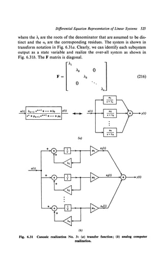
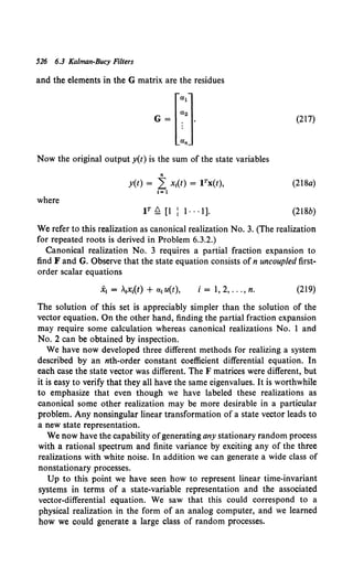
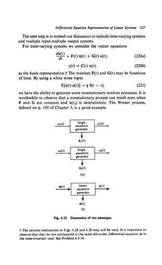
545. Differential Equation Representation ofLinear Systems 529
The resulting differential equations are
:i(t) = F(t) x(t) + G(t) u(t),
y(t) = C(t) x(t).
(233}
(234)
The driving function is a vector. For the message generation problem we
assume that the driving function is a white process with a matrix
covariance function
I E[u(t) uT(T)] £:! Q S(t - T), I (235)
where Q is a nonnegative definite matrix. The block diagram of the
generation process is shown in Fig. 6.33.
Observe that in general the initial conditions may be random variables.
Then, to specify the second-moment characteristics we must know the
covariance at the initial time
(236)
and the mean value E[x(t0)]. We can also generate coupled processes by
replacing the 0 matrices in (228), (229), or (231) with nonzero matrices.
The next step in our discussion is to consider the solution to (233).
We begin our discussion with the homogeneous time-invariant case. Then
(233) reduces to
:i(t) = Fx(t), (237)
with initial condition x(t0). If x(t) and F are scalars, the solution is
familiar,
x(t) = eF<t-to>x(t0). (238)
For the vector case we can show that (e.g. [27], [28], [29], or [30])
x(t) = eF<t-to> x(t0), (239)
x(t)
Matrix
time-varying gain
x(t) y(t)
Matrix
time-varying gain
Fig. 6.33 Message generation process.

546. 530 6.3 Kalman-Bucy Filters
where eFt is defined by the infinite series
F2t2
eFt Q I + Ft + 2f + ···. (240)
The function eF<t-tol is denoted by ~(t - t0) Q ~(r). The function
~(t - t0) is called the state transition matrix of the system. Two properties
can easily be verified for the time-invariant case.
Property ll.t The state transition matrix satisfies the equation
d~(t - t0) _ F"'-( )
--'--'-d--;1-= - 't" t - to (241)
or
d~~r) = F~(r). (242)
[Use (240) and its derivative on both sides of (239).]
Property 12. The initial condition
~(to - t0) = ~(0) = I (243)
follows directly from (239). The homogeneous solution can be rewritten
in terms of~(t - t0):
x(t) = ~(t - 10) x(t0). (244)
The solution to (242) is easily obtained by using conventional Laplace
transform techniques. Transforming (242), we have
s ~(s) - I = F ~(s), (245)
where the identity matrix arises from the initial condition in (243).
Rearranging terms, we have
or
[si - F] ~(s) = I
~(s) = (si - F)- 1 •
The state transition matrix is
A simple example illustrates the technique.
(246)
(247)
(248)
Example 4. Consider the system described by (206-210). The transform of the tran-
sition matrix is,
[ [1 0] [-p1 1]] -l
cZl(s) = s 0 1 - -Po 0 ' (249)
t Because we have to refer back to the properties at the beginning of the chapter we
use a consecutive numbering system to avoid confusion.

547. Differential Equation Representation ofLinear Systems 531
4>(s) = [s + P1 -1]-l,
Po s
(250)
4>(s) = 2 1 [ s 1 ] .
s + PlS + Po -Po s + Pl
(251)
To find cl»(T) we take the inverse transform. For simplicity we let p1 = 3 and
Po= 2. Then
[
2e- 2' - e-• : e-• - e- 2•]
ci»(T) = ----------+----------- • (252)
2[e- 2' - e-•]i 2e-• - e- 2•
It is important to observe that the complex natural frequencies involved
in the solution are determined by the denominator of4-(s). This is just the
determinant of the matrix sl - F. Therefore these frequencies are just the
roots of the equation
det [sl - F] = 0. (253)
For the time-varying case the basic concept of a state-transition matrix
is still valid, but some of the above properties no longer hold. From the
scalar case we know that~(t, t0) will be a function oftwo variables instead
ofjust the difference between t and t0 •
Definition. The state transition matrix is defined to be a function of two
variables ~(t, t0) which satisfies the differential equation
~(t, t0) = F(t)~(t, t0)
with initial condition ~(t0, t0) = I. The solution at any time is
x(t) = ~(t, t0) x(t0).
(254a)
(254b)
An analytic solution is normally difficult to obtain. Fortunately, in most
of the cases in which we use the transition matrix an analytic solution is
not necessary. Usually, we need only to know that it exists and that it has
certain properties. In the cases in which it actually needs evaluation, we
shall do it numerically.
Two properties follow easily:
and
~(t2, to) = ~(t2, t1)~(t1, to),
~ -l(t~o to) = ~(to, t1).
For the nonhomogeneous case the equation is
i(t) = F(t) x(t) + G(t) u(t).
The solution contains a homogeneous part and a particular part:
(255a)
(255b)
(256)
x(t) = ~(t, to) x(to) + r~(t, T) G('T) u('T) dT. (257)
Jt0

548. 532 6.3 Ka/man-Bucy Filters
(Substitute (257) into (256) to verify that it is the solution.) The output
y(t) is
y(t) = C(t) x(t). (258)
In our work in Chapters 4 and 5 and Section 6.1 we characterized time-
varying linear systems by their impulse response h(t, T). This characteriza-
tion assumes that the input is known from -oo to t. Thus
y(f) = f 00
h(f, T) U(T) dT. (259)
For most cases of interest the effect of the initial condition x( -oo) will
disappear in (257). Therefore, we may set them equal to zero and obtain,
y(t) = C(t) f"'cj>(t, r) G{r) u(r) dT.
Comparing (259) and (260), we have
h(t, T) = C(t)cj>(t, r) G(r),
0,
f 2: T,
elsewhere.
(260)
(261)
It is worthwhile to observe that the three matrices on the right will depend
on the state representation that we choose for the system, but the matrix
impulse response is unique. As pointed out earlier, the system is realizable.
This is reflected by the 0 in (261 ).
For the time-invariant case
and
Y(s) = H(s) V(s),
H(s) = C 4t(s)G.
(262)
(263)
Equation 262 assumes that the input has a Laplace transform. For a
stationary random process we would use the integrated transform (Section
3.6).
Most of our discussion up to this point has been valid for an arbitrary
driving function u(t). We now derive some statistical properties of vector
processes x(t) and y(t) for the specific case in which u(t) is a sample
function of a vector white noise process.
E[u(t) uT(T)] = Q o(t - r). (264)
Property 13. The cross correlation between the state vector x(t) of a
system driven by a zero-mean white noise u(t) and the input u(r) is
Kxu(t, T) ~ E[x(t) uT(r)].
It is a discontinuous function that equals
{
0,
Kxu(f, T) = !G(t)Q,
cj>(t, T) G(r)Q,
T > f,
T = (,
t0 < T < t.
(265)
(266)

549. Differential Equation Representation ofLinear Systems 533
Proof Substituting (257) into the definition in (265), we have
Kxu(t, r) = E{[cJ>(t, !0) x(t0) + 1:cJ>(t, a) G(a) u(a) da] uT(T)} (267)
Bringing the expectation inside the integral and assuming that the
initial state x(t0) is independent of u(r) for r > t0, we have
Kxu(t, r) = t cJ>(t, a) G(a) E[u(a) uT(r)] da
Jto
= (t cJ>(t, a) G(a) Q S(a - r) da.
Jt0
(268)
If r > t, this expression is zero. If r = t and we assume that the delta
function is symmetric because it is the limit of a covariance function, we
pick up only one half the area at the right end point. Thus
Kxu(f, t) = }cJ>(t, t) G(t)Q. (269)
Using the result following (254a), we obtain the second line in (266).
If r < t, we have
T < f (270a)
which is the third line in (266). A special case of (270a) that we shall use
later is obtained by letting r approach t from below.
lim Kxu(t, r) = G(t)Q. (270b)
The cross correlation between the output vector y(t) and u(r) follows
easily.
(271)
Property 14. The variance matrix of the state vector x(t) of a system
x(t) = F(t) x(t) + G(t) u(t)
satisfies the differential equation
with the initial condition
Ax(to) = E[x(t0) xT(t0)].
[Observe that Ax(t) = Kx(t, t).]
Proof
(272)
(274)
(275)

550. 534 6.3 Kalman-Bucy Filters
Differentiating, we have
dAx(t) = E [dx(t) xT(t)] + E [x(t) dxT(t)]. (276)
dt dt dt
The second term is just the transpose of the first. (Observe that x(t) is
not mean-square differentiable: therefore, we will have to be careful when
dealing with (276).]
Substituting (272) into the first term in (276) gives
E[d~;t) xT(t)] = E{[F(t) x(t) + G(t) u(t)] xT(t)}. (277)
Using Property l3 on the second term in (277), we have
E[d~~t) xT(t)] = F(t) Ax(t) + !G(t) Q GT(t). (278)
Using (278) and its transpose in (276) gives
Ax(t) = F(t) Ax(f) + Ax(t) FT(t) + G(t) Q GT(t), (279)
which is the desired result.
We now have developed the following ideas:
1. State variables of a linear dynamic system;
2. Analog computer realizations;
3. First-order vector differential equations and state-transition matrices;
4. Random process generation.
The next step is to apply these ideas to the linear estimation problem.
Observation Model. In this section we recast the linear modulation
problem described in the beginning of the chapter into state-variable
terminology. The basic linear modulation problem was illustrated in Fig.
6.1. A state-variable formulation for a simpler special case is given in
Fig. 6.34. The message a(t) is generated by passing y(t) through a linear
system, as discussed in the preceding section. Thus
i(t) = F(t) x(t) + G(t) u(t) (280)
and
(281)
For simplicity in the explanation we have assumed that the message of
interest is the first component of the state vector. The message is then
modulated by multiplying by the carrier c(t). In DSB-AM, c(t) would be
a sine wave. We include the carrier in the linear system by defining
C(t) = [c(t) !0: 0 0]. (282)

551. Differential Equation Representation ofLinear Systems 535
u(t)
n(t)
y(t)
L------------------------~
Message generation
Fig. 6.34 A simple case of linear modulation in the state-variable formulation.
Then
y(t) = C(t) x(t). (283)
We frequently refer to C(t) as the modulation matrix. (In the control
literature it is called the observation matrix.) The waveform y(t) is trans-
mitted over an additive white noise channel. Thus
where
r(t) = y(t) + w(t),
= C(t) x(t) + w(t),
T1 :5: t :5: T1
T,_ :5: t :5: T1,
E[w(t) w(7)] = ~o o(t - 7).
(284)
(285)
This particular model is too restrictive; therefore we generalize it in several
different ways. Two of the modifications are fundamental and we explain
them now. The others are deferred until Section 6.3.4 to avoid excess
notation at this point.
Modification No. 1: Colored Noise. In this case there is a colored noise
component nc(t) in addition to the white noise. We assume that the colored
noise can be generated by driving a finite-dimensional dynamic system
with white noise.
r(t) = CM(t) xM(t) + nc(t) + w(t).
The subscript M denotes message. We can write (286) in the form
r(t) = C(t) x(t) + w(t)
(286)
(287)

552. 536 6.3 Kalman-Bucy Filters
by augmenting the message state vector to include the colored noise
process. The new vector process x(t) consists of two parts. One is the
vector process xM(t) corresponding to the state variables of the system
used to generate the message process. The second is the vector process
xN(t) corresponding to the state variables of the system used to generate
the colored noise process. Thus
x(t) Q [~1!.1~~~]·
XN(t)
(288)
If xM(t) is n1-dimensional and xN(t) is n2-dimensional, then x(t) has
(n1 + n2) dimensions. The modulation matrix is
C(t) = [CM(t); CN(t)];
CM(t) is defined in (286) and CN(t) is chosen so that
nc(t) = CN(t) xN(t).
(289)
(290)
With these definitions, we obtain (287). A simple example is appropriate
at this point.
Example. Let
where
r(t) = V2P a(t)sin wet + ne(t) + w(t),
S ( ) 2kJ>A
G (d = 2 k 2'
(J) + G
-co < t, (291)
(292)
(293)
and ne(t), a(t), and w(t) are uncorrelated. To obtain a state representation we let
to =-co and assume that a(- co)= n.(- co)= 0. We define the state vector x(t) as
[a(t)]
x(t) = ·
ne(l)
(294)
Then,
[-k
F(t) = 0 G
_okJ· (295)
G(t) = [~ ~]. (296)
[2kaPa 0 ]
Q- .
0 2knPn
(297)
and
C(t) = (V2P sin wet : 1]. (298)
We see that F, G, and Q are diagonal because of the independence of the message
and the colored noise and the fact that each has only one pole. In the general case of
independent message and noise we can partition F, G, and Q and the off-diagonal
partitions will be zero.

553. Differential Equation Representation ofLinear Systems 537
Modification No. 2: Vector Channels. The next case we need to include to
get a general model is one in which we have multiple received waveforms.
As we would expect, this extension is straightforward. Assuming m
channels, we have a vector observation equation,
r(t) = C(t) x(t) + w(t). (299)
where r(t) ism-dimensional. An example illustrates this model.
Example. A simple diversity system is shown in Fig. 6.35. Suppose a(t) is a one-
dimensional process. Then x{t) = a(t). The modulation matrix is m x 1:
C(t) = r:~::J-
Cm(t)
(300)
The channel noises are white with zero-means but may be correlated with one
another. This correlation may be time-varying. The resulting covariance matrix is
E[w(t) wT(u)] Q R(t) 3(1 - u),
where R(t) is positive-definite.
(301)
In general, x(t) is ann-dimensional vector and the channel is m-dimen-
sional so that the modulation matrix is an m x n matrix. We assume that
the channel noise w(t) and the white process u(t) which generates the
message are uncorrelated.
With these two modifications our model is sufficiently general to include
most cases of interest. The next step is to derive a differential equation for
the optimum estimate. Before doing that we summarize the important
relations.
a(t)
Fig. 6.35 A simple diversity system.

554. 538 6.3 Kalman-Bucy Filters
Summary of Model
All processes are assumed to be generated by passing white noise through
a linear time-varying system. The processes are described by the vector-
differential equation
where
d~~) = F(t) x(t) + G(t) u(t),
E[u(t) uT(T)] = Q o(t - T).
(302)
(303)
and x(t0) is specified either as a deterministic vector or as a random vector
with known second-moment statistics.
The solution to (302) may be written in terms of a transition matrix:
The output process y(t) is obtained by a linear transformation of the
state vector. It is observed after being corrupted by additive white noise.
The received signal r(t) is described by the equation
Ir(t) = C(t) x(t) + w(t). I (305)
The measurement noise is white and is described by a covariance matrix:
E[w(t) wT(u)] = R(t) o(t - T). I (306)
Up to this point we have discussed only the second-moment properties
of the random processes generated by driving linear dynamic systems with
white noise. Clearly, if u(t) and w(t) are jointly Gaussian vector processes
and if x(t0) is a statistically independent Gaussian random vector, then the
Gaussian assumption on p. 471 will hold. (The independence of x(t0) is
only convenient, not necessary.)
The next step is to show how we can modify the optimum linear filtering
results we previously obtained to take advantage of this method of
representation.
6.3.2 Derivation of Estimator Equations
In this section we want to derive a differential equation whose solution is
the minimum mean-square estimate of the message (or messages). We
recall that the MMSE estimate of a vector x(t) is a vector i(t) whose com-
ponents .X1{t) are chosen so that the mean-square error in estimating each

555. Derivation of Estimator Equations 539
component is minimized. In other words, E[(x1(t) - x1(t))2], i = 1, 2, ... ,
n is minimized. This implies that the sum of the mean-square errors,
E{[xT(t) - xT(t)][x(t) - x(t)]} is also minimized. The derivation is straight-
forward but somewhat lengthy. It consists of four parts.
1. Starting with the vector Wiener-Hopf equation {Property 3A-V) for
realizable estimation, we derive a differential equation in t, with T as a
parameter, that the optimum filter h0(t, T) must satisfy. This is (317).
2. Because the optimum estimate i(t) is obtained by passing the
received signal into the optimum filter, (317) leads to a differential equation
that the optimum estimate must satisfy. This is (320). It turns out that all
the coefficients in this equation are known except b0(t, t).
3. The next step is to find an expression for h0{t, t). Property 4B-V
expresses b0 (t, t) in terms of the error matrix ;p(t). Thus we can equally
well find an expression for ;p(t). To do this we first find a differential
equation for the error x.(t). This is (325).
4. Finally, because
(307)
we can use (325) to find a matrix differential equation that ~p(t) must
satisfy. This is (330). We now carry out these four steps in detail.
Step I. We start with the integral equation obtained for the optimum
finite time point estimator [Property 3A-V, (52)]. We are estimating the
entire vector x(t)
Kx(t, o) CT(o) = rt ho(t, 'T) Kr('T, a) dT, T, < a < t, (308)
JT,
where
Differentiating both sides with respect to t, we have
T1 < a< t. (310)
First we consider the first term on the right-hand side of (310). For a < t
we see from (309) that
Kr{t, a) = C{t)[Kx(t, a)CT(a)], a < t. (311)
The term inside the bracket is just the left-hand side of (308). Therefore,
a < t. (312)

556. 540 6.3 Kalman-Bucy Filters
Now consider the first term on the left-hand side of (310),
oKx~:,a) = E[d~~t)xT(a)]. (313)
Using (302), we have
oKx~:· a) = F(t) Kx(t, a) + G(t) Kux(t, a), (314)
but the second term is zero for a < t [see (266)]. Using (308), we see that
F(t) Kx(t, a) CT(a) = Jt F(t) h0(t, T) Kr(T, a) dT. (315)
Tt
Substituting (315) and (312) into (310), we have
0 = I:.[-F(t) h0 (t, T) + h0 (t, t) C(t) h0 (t, T) + oho~i T)]Kr(T, a) dT,
T1 <a<t. (316)
Clearly, if the term in the bracket is zero for all T, T1 :::; T :::; t, (316) will
be satisfied. BecauseR(t) is positive-definite the condition is also necessary;
see Problem 6.3.19. Thus the differential equation satisfied by the optimum
impulse response is
oho~; T) = F(t) h.(t, T)- h.(t, t)C(t) h.(t, T). (317)
Step 2. The optimum estimate is obtained by passing the input through
the optimum filter. Thus
X(f) = s:. h0(t, T) f(T) dT. (318)
We assumed in (318) that the MMSE realizable estimate of x(T1) = 0.
Because there is no received data, our estimate at T1 is b.1sed on our a
priori knowledge. If x(T;) is a random variable with a mean-value vector
E[x(T1
)] and a covariance matrix Kx(T1, I;), then the MMSE estimate is
i(T;) = E[x(T1)].
If x(T1) is a deterministic quantity, say Xn(T1), then we may treat it as a
random variable whose mean equals Xn(t)
E[x(T;)] ~ Xn(t)
and whose covariance matrix Kx(Tt. T1) is identically zero.
Kx(T;, T;) ~ 0.

557. Derivation of Estimator Equations 541
In both cases (318) assumes E[x(T1)] = 0. The modification for other
initial conditions is straightforward (see Problem 6.3.20). Differentiating
(318), we have
(319)
Substituting (317) into the second term on the right-hand side of (319) and
using (318), we obtain
d~~) = F(t) i(t) + h0(t, t)[r(t) - C(t) i(t)]. (320)
It is convenient to introduce a new symbol for h0(t, t) to indicate that it is
only a function of one variable
z(t) Q h0(t, t). (321)
The operations in (322) can be represented by the matrix block diagram of
Fig. 6.36. We see that all the coefficients are known except z(t), but
Property 4C-V (53) expresses h0(t, t) in terms of the error matrix,
Iz(t) = h0(t, t) = ~p(t)CT(t) R-l(t). I (322)
Thus (320) will be completely determined if we can find an expression for
~p(t), the error covariance matrix for the optimum realizable point
estimator.
r(t)
___________,
l=....,=;;==i===;r==._ i(t)
Message generation
process
C(t) ~~=======~
l!::::======lmxn x(t)
Fig. 6.36 Feedback estimator structure.

558. 542 6.3 Kalman-Bucy Filters
Step 3. We first find a differential equation for the error x,(t), where
x,(t) ~ x(t) - i(t). (323)
Differentiating, we have
(324)
Substituting (302) for the first term on the right-hand side of (324), sub-
stituting (320) for the second term, and using (305), we obtain the desired
equation
dx (t)
-it = [F(t) - z(t) C(t)]x,(t) - z(t) w(t) + G(t) u(t). (325)
The last step is to derive a differential equation for ~p(t).
Step 4. Differentiating
~p(t) ~ E[x,(t) x,T(t)], (326)
we have
d~dlt) = E[dxd~t) x,T(t)] + E[x.(t) dx~(tl (327)
Substituting (325) into the first term of (327), we have
E[dxd~t) x/(t)] = E{[F(t)- z(t) C(t)] x,(t) x/(t)
- z(t) w(t) x/(t) + G(t) u(t) x/(t)}. (328)
Looking at (325), we see x,(t) is the state vector for a system driven by
the weighted sum of two independent white noises w(t) and u(t). Therefore
the expectations in the second and third terms are precisely the same type
as we evaluated in Property 13 (second line of 266).
E[dxd~t) x/(t)] = F(t);p(t) - z(t) C(t);p(t)
+ !z(t) R(t) zT(t) + ! G(t)Q GT(t). (329)
Adding the transpose and replacing z(t) with the right-hand side of (322),
we have
d~it) = F(t);p(t) + ;p(t) FT(t)- ;p(t) CT(t) R- 1(t) C(t);p(t)
+ G(t)Q GT(t), (330)
which is called the variance equation. This equation and the initial condition
(331)
determine ~p(t) uniquely. Using (322) we obtain z(t), the gain in the
optimal filter.

559. Derivation ofEstimator Equations 543
Observe that the variance equation does not contain the received signal.
Therefore it may be solved before any data is received and used to deter-
mine the gains in the optimum filter. The variance equation is a matrix
equation equivalent to n2 scalar differential equations. However, because
lgp(t) is a symmetric matrix, we have !n(n + 1) scalar nonlinear coupled
differential equations to solve. In the general case it is impossible to obtain
an explicit analytic solution, but this is unimportant because the equation
is in a form which may be integrated using either an analog or digital
computer.
The variance equation is a matrix Riccati equation whose properties
have been studied extensively in other contexts (e.g., McLachlan [31];
Levin [32]; Reid [33], [34]; or Coles [35]). To study its behavior adequately
requires more background than we have developed. Two properties are of
interest. The first deals with the infinite memory, stationary process case
(the Wiener problem) and the second deals with analytic solutions.
Property 15. Assume that T1 is fixed and that the matrices F, G, C, R, and
Q are constant. Under certain conditions, as t increases there will be an
initial transient period after which the filter gains will approach constant
values. Looking at (322) and (330), we see that as ~p(t) approaches zero
the error covariance matrix and gain matrix will approach constants. We
refer to the problem when the condition ~p(t) = 0 is true as the steady-
state estimation problem.
The left-hand side of (330) is then zero and the variance equation
becomes a set of !n(n + 1) quadratic algebraic equations. The non-
negative definite solution is ;p.
Some comments regarding this statement are necessary.
I. How do we tell if the steady-state problem is meaningful? To give
the best general answer requires notions that we have not developed [23].
A sufficient condition is that the message correspond to a stationary
random process.
2. For small n it is feasible to calculate the various solutions and select
the correct one. For even moderate n (e.g. n = 2) it is more practical to
solve (330) numerically. We may start with some arbitrary nonnegative
definite l;p(T1) and let the solution converge to the steady-state result (once
again see [23], Theorem 4, p. 8, for a precise statement).
3. Once again we observe that we can generate lgp(t) before the data is
received or in real time. As a simple example of generating the variance
using an analog computer, consider the equation:
(332)

560. 544 6.3 KD/man-Bucy Filters
(This will appear in Example 1.) A simple analog method of generation is
shown in Fig. 6.37. The initial condition is gp(T1) = P (see discussion in
the next paragraph).
4. To solve (or mechanize) the variance equation we must specify
;P(T1). There are several possibilities.
(a) The process may begin at T1 with a known value (i.e., zero
variance) or with a random value having a known variance.
(b) The process may have started at some time t0 which is much
earlier than T1 and reached a statistical steady state. In Property
14 on p. 533 we derived a differential equation that Ax(t) satisfied.
If it has reached a statistical steady state, Ax(t) = 0 and (273)
reduces to
0 = FAx + AxFT + GQGT. (333a)
This is an algebraic equation whose solution is Ax. Then
;p(T1) = A,. (333b)
if the process has reached steady state before T1• In order for the
unobserved process to reach statistical steady state (Ax(t) = 0),
it is necessary and sufficient that the eigenvalues of F have
negative real parts. This condition guarantees that the solution
to (333) is nonnegative definite.
In many cases the basic characterization of an unobserved
stationary process is in terms of its spectrum Sy{w). The elements
MO)=P
Fig. 6.37 Analog solution to variance equation.

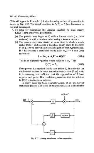
561. Derivation of Estimator Equations 545
in Ax follow easily from S11(w). As an example consider the state
vector in (191},
i = 1, 2, ... , n. (334a)
If y(t) is stationary, then
I"' dw
Ax,ll = Sll(w) -2
-"" 7T
(334b)
or, more generally,
Ax,lk = J:"" Uw)i+kSy(w) ~:· i = I, 2, ..., n, (334c)
k = I, 2, ... , n.
Note that, for this particular state vector,
Ax,lk = 0 when i + k is odd,
because Sy{w) is an even function.
(334d)
A second property ofthe variance equation enables us to obtain analytic
solutions in some cases (principally, the constant matrix, finite-time
problem). We do not use the details in the text but some of the problems
exploit them.
Property 16. The variance equation can be related to two simultaneous
linear equations,
dv~~t) = F(t) v1(t) + G(t) QGT(t) V2(t),
dv;~t) = CT(t) R-1(t) C(t) v1(t)- FT(t) v2(t),
or, equivalently,
Denote the transition matrix of (336) by
T(t, T1
) = [!!!~~·-~~-l-~~-~~~~~]·
T21(t, T,) : T22(t, T1)
Then we can show [32],
(335)
(337)
~p(t) = [T11(t, T1
) ~p(T1) + T12(t, T1
)][T21(t, T,} ~p(T,) + T22(t, T,)]- 1 • (338)

562. 546 6.3 Kalman-Bucy Filters
When the matrices of concern are constant, we can always find the transi-
tion matrix T (see Problem 6.3.21 for an example in which we find T by
using Laplace transform techniques. As discussed in that problem, we
must take the contour to the right of all the poles in order to include all
the eigenvalues) of the coefficient matrix in (336).
In this section we have transformed the optimum linear filtering problem
into a state variable formulation. All the quantities ofinterest are expressed
as outputs of dynamic systems. The three equations that describe these
dynamic systems are our principal results.
The Estimator Equation.
dx(t)
dt = F(t) x(t) + z(t)[r(t) - C(t) x(t)]. (339)
The Gain Equation.
(340)
The Variance Equation.
d'f,;;t) = F(t) 'f,p(t) + 'f,p(t) FT(t) - 'f,p(t) CT(t) R-l(t) C(t) 'f,p(t)
+ G(t) QGT(t). (341)
To illustrate their application we consider some simple examples, chosen
for one of three purposes:
1. To show an alternate approach to a problem that could be solved
by conventional Wiener theory.
2. To illustrate a problem that could not be solved by conventional
Wiener theory.
3. To develop a specific result that will be useful in the sequel.
6.3.3 Applications
In this section we consider some examples to illustrate the application
of the results derived in Section 6.3.2.
Example 1. Consider the first-order message spectrum
2kP
s.(w) = w2 + k2. (342)

563. Applications 547
In this case x(t) is a scalar; x(t) = a(t). Ifwe assume that the message is not modulated
and the measurement noise is white, then
r(t) = x(t) + w(t).
The necessary quantities follow by inspection:
F(t) = -k,
G(t) = 1,
C(t) = 1,
Q = 2kP,
No
R(t) = 2"
(343)
(344)
Substituting these quantities into (339), we obtain the differential equation for the
optimum estimate:
d!) = -kX(t) + z(t)[r(t) - X(t)]. (345)
The resulting filter is shown in Fig. 6.38. The value of the gain z(t) is determined by
solving the variance equation.
First, we assume that the estimator has reached steady state. Then the steady-state
solution to the variance equation can be obtained easily. Setting the left-hand side
of (341) equal to zero, we obtain
0 = -2k~Pao - ~~.. ;o+ 2kP.
where ~P .. denotes the steady-state variance.
~P.. !l lim Mt).
t~ao
(346)
There are two solutions to (346); one is positive and one is negative. Because ~P .. is
a mean-square error it must be positive. Therefore
No -v--
~Pao = k 2 (-1 + 1 + A) (347)
(recall that A = 4P/kNo). From (340)
z(oo) !l z.. = ~P.. R- 1 = k(-1 +VI+ A). (348)
r(t) x(t>
x(t)
Fig. 6.38 Optimum filter: example 1.

564. 548 6.3 Kalman-Bucy Filters
Clearly, the filter must be equivalent to the one obtained in the example in Section
6.2. The closed loop transfer function is
Ho(jw) = jw + Zkoo + Zoo
Substituting (348) in (349), we have
H( . >_ k<vi+A- 1)
0 }W - '
jw + kVl +A
which is the same as (94).
(349)
(350)
The transient problem can be solved analytically or numerically. The details of
the analytic solution are carried out in Problem 6.3.21 by using Property 16 on p. 545.
The transition matrix is
lcosh (yT) - ~sinh (yT) i 2kP sinh (yT) ]
y I y
T(T, + T, T.) = ---------------------:--------------------- •
N
2 sinh (yT) i cosh (yT) + ~sinh (p)
oY 1 Y
(351)
where
(352)
If we assume that the unobserved message is in a statistical steady state then .X (T,) = 0
and ~p(T,) = P. [(342) implies a{t) is zero-mean.] Using these assumptions and (351)
in (338), we obtain
~p(t + T,) = 2kP[ (y + k)e+yt + (y + k)e-yt] = 2kP (1 +
(y + k)2e+yt- (y- k)2e yt y + k 1
(353)
As t---+ w, we have
2kP No
l~n:l ~p(l + T,) = Y + k = T (y - k] = ~Pro, (354)
which agrees with (347). In Fig. 6.39 we show the behavior of the normalized error
as a function of time for various values of A. The number on the right end of each
curve is ~p( 1.2)- ~Pro. This is a measure of how close the error is to its steady-state value.
Example 2. A logical generalization of the one-pole case is the Butterworth family
defined in (153):
2nP sin (TT/2n)
Sa(w: n) = T (1 + (w/k)•·)· (355)
To formulate this equation in state-variable terms we need the differential equation of
the message generation process.
a<•>(t) + Pn-r a<•-U(t)+ ···+Po a(t) = u(t). (356)
The coefficients are tabulated for various n in circuit theory texts (e.g., Guillemin
[37] or Weinberg [38]). The values for k = 1 are shown in Fig. 6.40a. The pole
locations for various n are shown in Fig. 6.40b. If we are interested only in the

565. 0.9
0.8
0.7
0.6
~p(t)
0.5
0.4
0.3
0.2
n
2
3
4
5
6
7
Pn-l
1.414
2.000
2.613
3.236
3.864
4.494
F=-1
G=1
Q=2
C=1
1
R= 10
~p(O)= 1
t-+
Fig. 6.39 Mean-square error, one-pole spectrum.
Pn-2 Pn-3 Pn-4. Pn-5 Pn-6
1.000
2.000 1.000
3.414 2.613 1.000
5.236 5.236 3.236 1.000
7.464 9.141 7.464 3.864 1.000
10.103 14.606 14.606 10.103 4.494
aC•>(t) +Pn-lac•-I>(t) + ... +Poa(t) = u(t)
Pn-1
1.000
Fig. 6.40 (a) Coefficients in the differential equation describing the Butterworth
spectra [38).
549

566. 550 6.3 Kalman-Bucy Filters
jw jw
Unit
- -,<circle - .........
/ /
"'
/ ~
I I
I I
I
IT I IT
I
I
" ./ -'k.
*
-........
- ......... - /
n=l n=2
jw jw
#- '-.;::_ /~ -~
"
/ /
I ~ ~
I I
IT IT
I
~
I /
"~ /¥' " /
......... '.If- -*'
n=3 n=4
Poles are ats=exp{j7r(2m+n-l)}:m= 1,2, ..., 2n
Fig. 6.40 (b) pole plots, Butterworth spectra.
message process, we can choose any convenient state representation. An example is
defined by (191),
x1(t) = a(t)
x2(t) = a(t) = x1(t)
Xa(t) = a(t) = X2(t)
Xn(t) = a<n-ll(t) = Xn-1(1)
.Xn(t) = - I Pk- 1 a<k- 1>(t) + u(t)
k=l
= - I Pk-1 xk(t) + u(t)
k=l
(357)

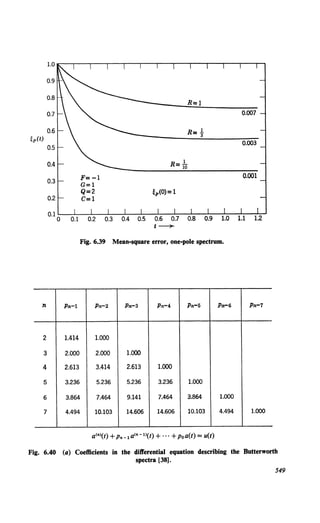
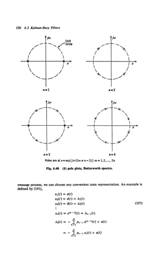
567. Applications 551
The resulting F matrix for any n is given by using (356) and (193). The other
quantities needed are
C(t) = [1 : 0 : . . . : 0]
Q = 2nPk2" -t sin (;,)
No
R(t) = 2 .
From (340) we observe that z(t) is an n x 1 matrix,
[
eu(t)]
z(t) = ~ g,~(t) •
No :
e,.(r>
.i,(t) = x2(t) + ;0eu(t)[r(t) - .X,{t)]
i 2(t) = x3(t) + ; 0
g,2 (t)[r(t) - x1(t)]
:i.(t) = -po.X,(t)- p,.X2(t)- ... -p._, x.(t) + ;0g,.{t)[r{t)- .X,(t)].
The block diagram is shown in Fig. 6.41.
Fig. 6.41 Optimum filter: nth-order Butterworth message.
(358)
(359)
(360)
(361)
(362)
(363)

568. 552 6.3 Kalman-Bucy Filters
0.9
0.7
0.008
hr(t)
0.002
R =Y.o 0.002
0] Q=2.tz
t -
0.2
R=~
0.1
0.9 1.0 1.1 1.2
t-+
Fig. 6.42 (a) Mean-square error, second-order Butterworth; (b) filter gains, second-
order Butterworth.
To find the values of tu(t), ... , t1n(t), we solve the variance equation. This could
be done analytically by using Property 16 on p. 545, but a numerical solution is much
more practical. We assume that T. = 0 and that the unobserved process is in a
statistical steady state. We use (334) to find fp(O). Note that our choice of state
variables causes (334d) to be satisfied. This is reflected by the zeros in !;p(O) as shown
in the figures. In Fig. 6.42a we show the error as a function of time for the two-pole
case. Once again the number on the right end of each curve is tP(1.2) - tp.,. We see
that for t = 1 the error has essentially reached its steady-state value. In Fig. 6.42b
we show the term t12Ct). Similar results are shown for the three-pole and four-pole
cases in Figs. 6.43 and 6.44, respectively.t In all cases steady state is essentially
reached by t = I. (Observe that k = 1 so our time scale is normalized.) This means
t The numerical results in Figs. 6.39 and 6.41 through 6.44 are due to Baggeroer [36].

569. 0.8
0.7
0.6
Eu(t)
0.5
0.3
0.2
0.1
0
0.3
0.2
~12(t)
0.1
0
-0.6
~la(t) _ 0.3
-0.2
-0.1
1
0
-2
t -
0.1
(Note negative scale)
t --;.-
Fig. 6.43 (a) Mean-square error, tbird-order Butterworth; (b) filter gain, tbird-order
Butterworth; {c) filter gain, tbird-order Butterworth.
553

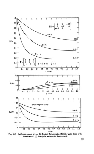
570. tp(O)=[ ~ 0 -0.414
-0.~14]
0.1 0.414 0
-0.414 0 0.414
0 -0.414 0
0
0 0.1 0.2 0.3 0.4 0.5 0.6
t -
0.2
~~ 1
!dt) ··: 1...-,j;;;'iiiiii!i~~:::::i::=:=:L._J..__l
_ _!__
R_=--l:-Yt-o--:1:1-,-LI:-R-=~~--1=-=-=-•
~
0.1 0.2 0.3 0.4 0.5 0.6 0.7 0.8 0.9 1.0 1.1 1.2
t-;..
-0.3
6a(t)
-0.2
Fig. 6.44 (a) Mean-square error, fourth-order Butterworth; (b) filter gains, fourth-
order Butterworth; (c) filter gains, fourth-order Butterworth.
554

571. Applications 555
-2.5 .------.--,---.---r--~-.----.---.--.--..---.----.---,
-2.0
~l4(t)
-1.:L~~~~~§§§§~~=~=~~=~~~:J
0.1 0.2
t -
Fig. 6.44 (d) filter gains, fourth-order Butterworth.
that after t = I the filters are essentially time-invariant. (This does not imply that all
terms in ~p(t) have reached steady state.) A related question, which we leave as an
exercise, is, "If we use a time-invariant filter designed for the steady-state gains, how
will its performance during the initial transient compare with the optimum time-
varying filter?" (See Problems 6.3.23 and 6.3.26.)
Example 3. The two preceding examples dealt with stationary processes. A simple
nonstationary process is the Wiener process. It can be represented in differential
equation form as
x(t) = G u(t),
x(O) = 0.
(364)
Observe that even though the coefficients in the differential equation are constant
the process is nonstationary. If we assume that
r(t) = x(t) + w(t), (365)
the estimator follows easily
f(t) = z(t)[r(t) - x(t)], (366)
where
2
z(t) =No Mt) (367)
and
(368)
The transient problem can be solved easily by using Property 16 on p. 545 (see
Problem 6.3.25). The result is
(369)
where r = [2G2 Q/N0 ]Y.. [Observe that (369) is not a limiting case of (353) because the
initial condition is different.] As t---+ oo, the error approaches steady state.
~1'.. = (~0 G2Qr (370)
[(370) can also be obtained directly from (368) by letting ep(t) = 0.)

572. 556 6.3 Kalman-Bucy Filters
r(t) -J2G2Q/No x(t)
+ s
+
-
x(t)
Fig. 6.45 Steady-state filter: Example 3.
The steady-state filter is shown in Fig. 6.45. It is interesting to observe that this
problem is not included in the Wiener-Hopf model in Section 6.2. A heuristic way to
include it is to write
G"Q
S,(w) = - 2 - -
2 •
w + €
(371)
solve the problem by using spectral factorization techniques, and then let f ->- 0.
It is easy to verify that this approach gives the system shown in Fig. 6.45.
Example 4. In this example we derive a canonic receiver model for the following
problem:
1. The message has a rational spectrum in which the order of the numerator as a
function of w• is at least one smaller than the order of the denominator. We use the
state variable model described in Fig. 6.30. The F and G matrices are given by (212)
and (213), respectively (Canonic Realization No. 2).
2. The received signal is scalar function.
3. The modulation matrix has unity in its first column and zero elsewhere. In
other words, only the unmodulated message would be observed in the absence of
measurement noise,
C(t) = [1 : 0 · · · 0]. (372)
The equation describing the estimator is obtained from (339),
i(t) = Fi(t) + z(t)[r(t} - x1(t)] (373)
and
(374)
As in Example 2, the gains are simply 2/No times the first row of the error matrix.
The resulting filter structure is shown in Fig. 6.46. As t->- oo, the gains become
constant.
For the constant-gain case, by comparing the system inside the block to the two
diagrams in Fig. 6.30 and 31a, we obtain the equivalent filter structure shown in
Fig. 6.47.
Writing the loop filter in terms of its transfer function, we have
2 ~us"- 1 + ···+ ~'"
G,.(s) = No s• + Pn-1S" 1 +···+Po.
(375)

573. a(t)
Applications 557
,----------------------,
I I
I I
I
I
I
I
I
I
I
I
x(t) 1
I a(t)
I
I
I
I
I
I I
I :
L----------------------~
Loop filter
Fig. 6.46 Canonic estimator: stationary messages, statistical steady-state.
Thus the coefficients of the numerator of the loop-filter transfer function correspond
to the first column in the error matrix. The poles (as we have seen before) are identical
to those of the message spectrum.
Observe that we still have to solve the variance equation to obtain the numerator
coefficients.
Example SA [23]. As a simple example of the general case just discussed, consider
the message process shown in Fig. 6.48a. If we want to use the canonic receiver
structure we have just derived, we can redraw the message generator process as shown
in Fig. 6.48b.
We see that
p, = k, Po= 0, b, = 0, bo = 1. (376)
~11 S n-l + "• + ~ln
Fig. 6.47 Canonic estimator: stationary messages, statistical steady-state.

574. 558 6.3 Kalman-Bucy Filters
u(t)
u(t) ----~~~ ~
(a)
(b)
x1(t) =a(tJ
(c)
1------) a(t)
x!(t) = a(t)
x1CtJ a(t)
Fig. 6.48 Systems for example SA: (a) message generator; (b) analog representation;
(c) optimum estimator.
Then, using (212) and (213), we have
F = [~k ~]. G = [~]. c = [1 0] (377)
Q = q, R = No/2.
The resulting filter is just a special case of Fig. 6.47 as shown in Fig. 6.48.

575. The variance equation in the steady state is
2( -k~n + ~12) - ~0 ~112 = 0,
2
-k~12 + e22 - No eue12 = 0,
2 1: 2
No H2 = q.
Thus the steady-state errors are
e12 = No (2q)*
2 No
Applications 559
(378)
(379)
We have taken the positive definite solution. The loop filter for the steady-state case
is
(380)
Example 5B. An interesting example related to the preceding one is shown in Fig.
6.49. We now add A and B subscripts to denote quantities in Examples SA and SB,
respectively. We see that, except for some constants, the output is the same as in
Example 5A. The intermediate variable x.8 (t), however, did not appear in that
realization.
We assume that the message of interest is x28 (t). In Chapter 11.2 we shall see the
model in Fig. 6.49 and the resulting estimator play an important role in the FM
problem. This is just a particular example of the general problem in which the
message is subjected to a linear operation before transmission. There are two easy
ways to solve this problem. One way is to observe that because we have already
solved Example 5A we can use that result to obtain the answer. To use it we must
express x28 (t) as a linear transformation of x1A(t) and x.A(t), the state variables in
Example SA.
and
if we require
Observing that
we obtain
u(t)
Fig. 6.49 Message generation, example SB.
(381)
(382)
(383)
(384)
(38S)

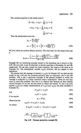
576. 560 6.3 Kalman-Bucy Filters
Now minimum mean-square error filtering commutes over linear transformations.
(The proof is identical to the proof of 2.237.) Therefore
(386)
Observe that this is not equivalent to letting f1x2s(t) equal the derivative of .X1A(t). Thus
(387)
With these observations we may draw the optimum filter by modifying Fig. 6.48.
The result is shown in Fig. 6.50. The error variance follows easily:
(388)
Alternatively, if we had not solved Example SA, we would approach the problem
directly. We identify the message as one of the state variables. The appropriate
matrices are
G = [~]. c = [l 0) (389)
and
Q = Qs. (390)
r(t)
+
Fig. 6.50 Estimator for example 58.

577. Applications 561
The structure of the estimator is shown in Fig. 6.51. The variance equation is
2
t12(t) = /3~22(t) - M12(t) - No ~u(t)~12(t), (391)
t22(t) = -2k~22(t) - ~0 ~Mt) + qs.
Even in the steady state, these equations appear difficult to solve analytically. In
this particular case we are helped by having just solved Example SA. Clearly, ~11(1)
must be the same in both cases, if we let qA = f32q8• From (379)
kN0 { [ 2 (2q8 f32
)*]*}
~ll,a> =2 -1 + 1 + k2 N;;
~:,. kNo~<.
- 2
The other gain ~12,oo now follows easily
(392)
(393)
Because we have assumed that the message of interest is x2(t), we can also easily
calculate its error variance:
(394)
It is straightforward to verify that (388) and (394) give the same result and that the
block diagrams in Figs. 6.50 and 6.51 have identical responses between r(t) and x2(t).
The internal difference in the two systems developed from the two different state
representations we chose.
r(t)
+
Fig. 6.51 Optimum estimator: example SB (form #2).

578. 562 6.3 Kalman-Bucy Filters
Example 6. Now consider the same message process as in Example I but assume that
the noise consists of the sum of a white noise and an uncorrelated colored noise,
n(t) = nc(t) + w(t) (395)
and
(396)
As already discussed, we simply include nc(t) as a component in the state vector.
Thus,
and
and
x(t) _ ,
t:,. [a(t) ]
nc(t)
F(t) = [ -k 0 ]
0 -kc '
G(t) = [
1 0
]
0 1 '
C(t) = [1 1],
[
2kP
Q(r) = 0
R(t) =No.
2
The gain matrix z(t) becomes
or
2
Zu(t) = No [~u(t) + ~12(t)],
2
Z21(t) = No [~12(t) + ~22(t)].
The equation specifying the estimator is
d~~) = F(t) i(t) + z(t)[r(t) - C(t) i(t)],
or in terms of the components
dx~~t) = -kX1(t) + z11(t)[r(t) - x1(t) - x2(t)],
dx;~t) = -kcx2(t) + Z21(t)[r(t) - x1(t) - X2(t)].
(397)
(398)
(399)
(400)
(401)
(402)
(403)
(404)
(405)
(406)
(407)
(408)
The structure is shown in Fig. 6.52a. This form of the structure exhibits the
symmetry of the estimation process. Observe that the estimates are coupled through
the feedback path.

579. Applications 563
~.(tJ = a(t)
H-.....------.
(a)
r(t)
+
(b)
Fig. 6.52 Optimum estimator: colored and white noise (statistical steady-state).
An equivalent asymmetrical structure which shows the effect of the colored noise
on the message is shown in Fig. 6.52b. To find the gains we must solve the variance
equation. Substituting into (341), we find
2
~u(t) = - 2keu(t) - No (eu(t) + e12(t))2 + 2kP, (409)
. 2
~12(t) = - (k + kc)~dt) - No (gu(t) + ~12(t))a12(t) + '22(t)), (410)
~dt) = - 2kc~dt) - ~o {el2(t) + e22(t))2 + 2kcPc. (411)
Two comments are in order.
1. The system in Fig. 6.52a exhibits all of the essential features of the canonic
structure for estimating a set of independent random processes whose sum is observed

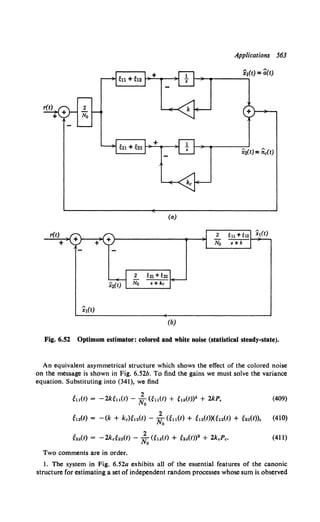
580. 564 6.3 Kalman-Bucy Filters
in the presence of white noise (see Problem 6.3.31 for a derivation of the general
canonical structure). In the general case, the coupling arises in exactly the same
manner.
2. We are tempted to approach the case when there is no white noise (No = 0)
with a limiting operation. The difficulty is that the variance equation degenerates.
A derivation of the receiver structure for the pure colored noise case is discussed in
Section 6.3.4.
Example 7. The most common example of a multiple observation case in com-
munications is a diversity system. A simplified version is given here. Assume that the
message is transmitted over m channels with known gains as shown in Fig. 6.53.
Each channel is corrupted by white noise. The modulation matrix is m x n, but only
the first column is nonzero:
[
c2 ; l
C(t) = ~2 : 0 ~ [c : 0].
Cm ,
(412)
For simplicity we assume first that the channel noises are uncorrelated. Therefore
R(t) is diagonal:
N1
2 0
N2
R(t) = T (413)
0 Nm
T
Cl Wl(t)
r1(t)
C2 W2(t)
r2(t)
a(t)
Cm Wm(t)
r----- rm(t)
Fig. 6.53 Diversity system.

581. The gain matrix z(t) is an n x m matrix whose ijth element is
2ct t )
Ztf(t) = Nt sn(t .
Applications 565
(414)
The general receiver structure is shown in Fig. 6.54a. We denote the input to the
inner loop as v(t),
v(t) = z(t)[r(t) - C(t) x(t)]. (415a)
Using (412)-(414), we have
[
m 2c
v,(t) = 'n(t) 2 Nf rlt) -
!=1 j
( m 2c 2) ]
2 ,J x1 (t) 0
!= 1 j
(415b)
We see that the first term in the bracket represents a no-memory combiner of the
received waveforms.
Denote the output of this combiner by rc(t),
m 2Ct
rc(t) = L N rt{t).
1=1 f
(416)
We see that it is precisely the maximal-ratio-combiner that we have already en-
countered in Chapter 4. The optimum filter may be redrawn as shown in Fig. 6.54b.
We see that the problem is reduced to a single channel problem with the received
waveform rc(t),
r(t)
r(t)
(
m 2c 2 ) m 2c
rc(t) = 2 tJ- a(t) + 2 Nf n1(t).
1=1 f !=1 f
c
x(t)
(a)
m
~ 1-c.2
...:;, N· '
i=l 1
(b)
Fig. 6.54 Diversity receiver.
(417a)
x(t)

582. 566 6.3 Kalman-Bucy Filters
The modulation matrix is a scalar
(
m 2c 2)
c= .L-1.
1=1 N1
(417b)
and the noise is
(417c)
If the message a(t) has unity variance then we have an effective power of
(
m 2 )2
Per= LN cl
1=1 1
(418)
and an effective noise level of
(419)
Therefore all of the results for the single channel can be used with a simple scale
change; for example, for the one-pole message spectrum in Example 1 we would have
(420)
where
A r = ~ ~ 2c12
=! ~ 2PI,
• k 1=1 N1 k 1=1 N1
(421)
Similar results hold when R(t) is not diagonal and when the message is nonstationary.
These seven examples illustrate the problems encountered most fre-
quently in the communications area. Other examples are included in the
problems.
6.3.4 Generalizations
Several generalizations are necessary in order to include other problems
of interest. We discuss them briefly in this section.
Prediction. In this case d(t) = x(t + a), where a is positive. We can
show easily that
d(t) = cp(t + a, t) i(t), a> 0,
where cp(t, T) is the transition matrix of the system,
x(t) = F(t) x(t) + G(t) u(t)
(see Problem 6.3.37).
When we deal with a constant parameter system,
cp(t + a, t) = fiF«,
and (422) becomes
a(t) = eF« x(t).
(422)
(423)
(424)
(425)

583. Generalizations 567
Filtering with Delay. In this case d(t) = x(t + a), but a is negative.
From our discussions we know that considerable improvement is available
and we would like to include it. The modification is not so straightforward
as the prediction case. It turns out that the canonic receiver first finds the
realizable estimate and then uses it to obtain the desired estimate. A good
reference for this type of problem is Baggeroer [40]. The problem of
estimating x(t1), where t1 is a point interior to a fixed observation interval,
is also discussed in this reference. These problems are the state-variable
counterparts to the unrealizable filters discussed in Section 6.2.3 (see
Problem 6.6.4).
Linear Transformations on the State Vector. If d(t) is a linear trans-
formation of the state variables x(t), that is,
d(t) = ka(t) x(t), (426)
then
d(t) = ka(t) i(t). (427)
Observe that ka(t) is not a linear filter. It is a linear transformation of the
state variables. This is simply a statement of the fact that minimum mean-
square estimation and linear transformation commute. The error matrix
follows easily,
;d(t) ~ E[(d(t) - d(t))(dT(t) - dT(t))] = kit) ;p(t) kaT(t). (428)
In Example 5B we used this technique.
Desired Linear Operations. In many cases the desired signal is obtained
by passing x(t) or y(t) through a linear filter. This is shown in Fig. 6.55.
Desired
= linear d(t)
operation
I Message I
==~I t• t==~=="==={. X j)===j~y(t)
u(t) genera 1on 1 x(t) , -
C(t)
Fig. 6.55 Desired linear operations.

584. 568 6.3 Kalman-Bucy Filters
Three types of linear operations are of interest.
1. Operations such as differentiation; for example,
d
d(t) = dt x1(t). (429)
This expression is meaningful only if x1(t) is a sample function from a
mean-square differentiable process.t If this is true, we can always choose
d(t) as one of the components of the message state vector and the results
in Section 6.3.2 are immediately applicable. Observe that
(430)
In other words, linear filtering and realizable estimation do not commute.
The result in (430) is obvious if we look at the estimator structure in
Fig. 6.51.
2. Improper operations; for example, assume y(t) is a scalar function and
d(t) = L"' ka(r)y(t- r) dr, (43la)
where
. jw + ex ex - f3
Ka(Jw) = -.-- = 1 + -.--·
jw + f3 jW + f3
(43lb)
In this case the desired signal is the sum of two terms. The first term is
y(t). The second term is the output of a convolution operation on the past
of y(t). In general, an improper operation consists of a weighted sum of
y(t) and its derivatives plus an operation with memory. To get a state
representation we must modify our results slightly. We denote the state
vector of the dynamic system whose impulse response is ka(T) as xa(t).
(Here it is a scalar.) Then we have
.Xa(t) = -f3xa(t) + y(t) (432)
and
d(t) = (ex - {3) xd(t) + y(t).
Thus the output equation contains an extra term. In general,
ia(t) = Fa(t) xa(t) + Ga(t) x(t),
d(t) = Ca(t) xa(t) + Ba(t) x(t).
(433)
(434)
(435)
Looking at (435) we see that if we augment the state-vector so that it
contains both xit) and x(t) then (427) will be valid. We define an
augmented state vector
[ x(t) J
Xa(t) ~ ----- •
xd(t)
(436)
t Note that we have>worked with x(t) when one of its components was not differen-
tiable. However the output of the system always existed in the mean-square sense.

585. Generalizations 569
The equation for the augmented process is
[ F(t) : 0 J [G(t)J
xa{t) = ·----- -----· Xa(t) + ---- u(t).
Ga(t): Fit) 0
(437)
The observation equation is unchanged:
r(t) = C(t) x(t) + w(t); (438)
However we must rewrite this in terms of the augmented state vector
r(t) = Ca(t) Xa(t) + w(t), (439)
where
Ca{t) ~ [C(t) l 0]. (440)
Now d(t) is obtained by a linear transformation on the augmented state
vector. Thus
d(t) = Ca(t) X:a(t) + Ba(t) x(t) = [Ba(t) : Ca(t)][xa(t)]. (441)
(See Problem 6.3.41 for a simple example.)
3. Proper operation: In this case the impulse response of kir) does not
contain any impulses or derivatives of impulses. The comments for the
improper case apply directly by letting Ba{t) = 0.
Linear Filtering Before Transmission. Here the message is passed through
a linear filter before transmission, as shown in Fig. 6.56. All comments
for the preceding case apply with obvious modification; for example,
if the linear filter is an improper operation, we can write
x1(t) = F1(t) x1(t) + G1(t) x(t),
y1(t) = C1(t) x1(t) + B1(t) x(t).
Then the augmented state vector is
w(t)
x(t)
F======1~ + )===~
y1 (t) r(t)
Fig. 6.56 Linear filtering before transmission.
(442)
(443)
(444)

586. 570 6.3 Kalman-Bucy Filters
The equation for the augmented process is
X4 (t) = [~~)--~ ·--~--]X4 (t) + [?-~~] u(t).
Gf(t) I F/(t) 0
(445)
The observation equation is modified to give
r(t) = yt<t) + w(t) = [B1(t) : Ct(t)][~~)_] + w(t).
I Xt(t)
(446)
For the last two cases the key to the solution is the augmented state vector.
Correlation Between u(t) and w(t). We encounter cases in practice in
which the vector white noise process u(t) that generates the message is
correlated with the vector observation noise w(t). The modification in the
derivation of the optimum estimator is straightforward.t Looking at the
original derivation, we find that the results for the first two steps are
unchanged. Thus
i(t) = F(t) x(t) + h0 (t, t)[r(t) - C(t) x(t)]. (447)
In the case of correlated u(t) and w(t) the expression for
z(t) ~ h0(t, t) ~ lim ho(t, u) (448)
must be modified. From Property 3A-V and the definition of;p(t) we have
;p(t) = ul~~ [Kx(t, u) - J:, h0 (t, T) Krx(T, u) dT]. (449)
Multiplying by CT(t),
;p(t) CT(t) = lim [Kx(t, u) CT(t) - (' h0 (t, T) Krx(T, U) CT(t)dT ]
u....t- JT,
= lim [Kxr(t, u) - Kxw(t, u) - rt ho(t, T) Krx(T, u) CT(u) dT.]
u-t- JT,
Now, the vector Wiener-Hopf equation implies that
}~~ Kxr(t, u) = }~~ [J;,h0 (t, T) Kr(T, u) dT]
= lim u:.ho(t, T)[Krx(T, u) CT(u) + R(T) o(T- u)
+ C(T)Kxw (T, U)] dTl
(450)
(451)
t This particular case was first considered in [41 ]. Our derivation follows Collins [42].

587. Generalizations 571
Using (451) in (450), we obtain
;p(t) CT(t) = lim [ho(t, u)R(u) + rt ho(t, T) C(T) Kxw(T, u) dT- Kxw(t, u)].
u->t- JT,
(452)
The first term is continuous. The second term is zero in the limit because
Kxw(T, u) is zero except when u = t. Due to the continuity of h0 (t, T) the
integral is zero. The third term represents the effect of the correlation.
Thus
;p(t)C(t) = h0 (t, t) R(t) - lim Kxw(t, u). (453)
u-+t-
Using Property 13 on p. 532, we have
lim Kxw(t, u) = G(t) P(t), (454)
u-t-
where
(455)
Then
z(t) ~ h0(t, t) = [~p(t) CT(t) + G(t) P(t)]R- 1(t). (456)
The final step is to modify the variance equation. Looking at (328), we
see that we have to evaluate the expectation
E{[ -z(t) w(t) + G(t) u(t)]x/(t)}.
To do this we define a new white-noise driving function
v(t) ~ -z(t) w(t) + G(t) u(t).
Then
E[v(t)vT(T)] = [z(t)R(t)zT(t) + G(t)QGT(t)]8(t - T)
(457)
(458)
- [z(t)E[w(t)uT(t)]GT(t) + G(t)E[u(t)wT(t)]zT(t)] (459)
or
E[v(t) vT(T)] = [z(t) R(t) zT(t) - z(t) PT(t) GT(t) - G(t) P(t)zT(t)
+ G(t) QGT(t)] 8(t - T) ~ M(t) 8(t - T), (460)
and, using Property 13 on p. 532, we have
E[(-z(t) w(t) + G(t) u(t))x/(t)] = !M(t). (461)
Substituting into the variance equation (327), we have
~p(t) = {F(t);p(t) - z(t) C(t);p(t)} + {,..,V
+ z(t) R(t) zT(t) - z(t) PT(t) GT(t)
- G(t) P(t) zT(t) + GT(t) Q GT(t). (462)

588. 572 6.3 Kalman-Bucy Filters
Using the expression in (456) for z(t), (462) reduces to
~p(t) = [F(t) - G(t) P(t) R - 1(t) C(t)] ;p(t)
+ ~p(t)[FT(t) - CT(t) R -l(t)PT(t)G(t)]
- ;p(t) CT(t) R -l(t) C(t);p(t)
+ G(t)[Q- P(t) R- 1(t)PT(t)] GT(t),
(463)
which is the desired result. Comparing (463) with the conventional variance
equation (341), we see that we have exactly the same structure. The
correlated noise has the same effect as changing F(t) and Q in (330). If
we define
and
F.,(t) ~ F(t)- G(t) P(t) R- 1(t) C(t)
Q.,(t) ~ Q- P(t)R- 1(t)PT(t),
(464)
(465)
we can use (341) directly. Observe that the filter structure is identical to
the case without correlation; only the time-varying gain z(t) is changed.
This is the first time we have encountered a time-varying Q(t). The results
in (339)-(341) are all valid for this case. Some interesting cases in which
this correlation occurs are included in the problems.
Colored Noise Only. Throughout our discussion we have assumed that
a nonzero white noise component is present. In the detection problem we
encountered cases in which the removal of this assumption led to singular
tests. Thus, even though the assumption is justified on physical grounds, it
is worthwhile to investigate the case in which there is no white noise
component. We begin our discussion with a simple example.
Example. The message process generation is described by the differential equation
(466)
The colored-noise generation is described by the differential equation
(467)
The observation process is the sum of these two processes:
y(t) = x1(t) + x 2(t). (468)
Observe that there is no white noise present. Our previous work with whitening
filters suggests that in one procedure we could pass y(t) through a filter designed so
that the output due to x2(t) would be white. (Note that we whiten only the colored
noise, not the entire input.) Looking at (468), we see that the desired output is
y(t) - F2(t)y(t). Denoting this new output as r'(t), we have
r'(t)!::. y(t) - F2(t) y(t)
= x1(t) - F.(t) x1(t) + G.(t) u.(t), (469)
r'(t) = [F1(t) - F.(t)]xl(t) + w'(t), (470)

589. Generalizations 573
where
w'(t) ~ G1(t) u1(t) + G2(t) u2(t).
We now have the problem in a familiar format:
r'(t) = C(t) x(t) + w'(t),
where
C(t) = [F1 (t) - F2(t) j 0).
The state equation is
[xl(t)] = [F1(t)
x2(t) o
0 ] [x1(t)] [G1(t) 0 ] [u1(t)]
F2(t) x2(t) + 0 G2(t) u2(t) .
We observe that the observation noise w'(t) is correlated with u(t).
E[u(t) w'(T)] = ll(t - T) P(t),
so that
(471)
(472)
(473)
(474)
(475)
(476)
The optimal filter follows easily by using the gain equation (456) and the variance
equation (463) derived in the last section. The general caset is somewhat more
complicated but the basic ideas carry through (e.g., [43], [41], or Problem 6.3.45).
Sensitivity. In all of our discussion we have assumed that the matrices
F(t), G(t), C(t), Q, and R(t) were known exactly. In practice, the actual
matrices may be different from those assumed. The sensitivity problem is
to find the increase in error when the actual matrices are different. We
assume the following model:
Xmo(t) = Fmo(f) Xmo(f) + Gmo(f) Umo(t),
fmo(t) = Cmo(t) Xmo(t) + Wmo(t).
(477)
(478)
The correlation matrices are Qmo and Rmo(t). We denote the error matrix
under the model assumptions as!;mo(t).(The subscript"mo"denotesmodel.)
Now assume that the actual situation is described by the equations,
Xac(t) = Fac(l) Xac(t) + Gac(t) Uac(t),
fac(t) = Cac(l) Xac(l) + Wac(!),
(479)
(480)
t We have glossed over two important issues because the colored-noise-only problem
does not occur frequently enough to warrant a lengthy discussion. The first issue is
the minimal dimensionality of the problem. In this example, by a suitable choice of
state variables, we can end up with a scalar variance equation instead of a 2 x 2
equation. We then retrieve x(t) by a linear transformation on our estimate of the
state variable for the minimal dimensional system and the received signal. The
second issue is that of initial conditions in the variance equation. l;p(O-) may not
equal !;p(O + ). The intereste,d reader should consult the two references listed for a
more detailed discussion.

590. 574 6.3 Kalman-Bucy Filters
with correlation matrices Qac and Rac(t). We want to find the actual
error covariance matrix ;ac(t) for a system which is optimum under the
model assumptions when the input is rac(t). (The subscript "ac" denotes
actual.) The derivation is carried out in detail in [44]. The results are given
in (484)-(487). We define the quantities:
~ac(t) ~ E[x.ac(t) xrao(t)],
~a.(t) ~ E[Xac(t) xrao(t)],
F.(t) ~ Fac(t) - Fmo(t).
C.(t) ~ Cac(t) - Cmo(t).
(481)
(482)
(483a)
(483b)
The actual error covariance matrix is specified by three matrix equations:
~ac(t) = {[Fmo(t) - ;mo(t) Cm/(t) Rmo-l(t) Cm0 (t)] ;ac(t)
- [F,(t) - ;mo(t) Cm/(t) Rmo-l(t) C,(t)] ;a.(t)}
+ {""' JT + Gac(t) Qac Ga/(t)
+ ;mo{t) CmoT(t) Rmo-l(t) Rac(t) Rmo-l(t) Cmo(t) ;mo(t), (484)
~a.(t) = Fac(t) ;a,(t) + ;a,(t) FmoT(t)
- ~aE(t) Cm/(t) Rmo -l(t) Cm0 (1) ~m0(t)
- Aac(t) Fl(t) + Aac(t) C,T(t) Rmo-l(t) Cmo(t) ;mo(t)
+ Gac(t) Qac Ga/(t), (485)
where
Aac(l) ~ E[Xa0 (!) Xa/(t)]
satisfies the familiar linear equation
(486)
Aac(t) = Fac(l) Aac(t) + Aac(t) Fa/(t) + Gac(t) Qac Ga/(t). (487)
We observe that we can solve (487) then (485) and (484). In other words
the equations are coupled in only one direction. Solving in this manner
and assuming that the variance equation for ~mo(t) has already been
solved, we see that the equations are linear and time-varying. Some typical
examples are discussed in [44] and the problems.
Summary
With the inclusion of these generalizations, the feedback filter formula-
tion can accommodate all the problems that we can solve by using con-
ventional Wiener theory. (A possible exception is a stationary process with
a nonrational spectrum. In theory, the spectral factorization techniques
will work for nonrational spectra if they satisfy the Paley-Wiener criterion,
but the actual solution is not practical to carry out in most cases of
interest).

591. Summary 575
We summarize some ofthe advantages ofthe state-variable formulation.
I. Because it is a time-domain formulation, nonstationary processes
and finite time intervals are easily included.
2. The form of the solution is such that it can be implemented on a
computer. This advantage should not be underestimated. Frequently,
when a problem is simple enough to solve analytically, our intuition is
good enough so that the optimum processor will turn out to be only
slightly better than a logically designed, but ad hoc, processor. However,
as the complexity of the model increases, our intuition will start to break
down, and the optimum scheme is frequently essential as a guide to design.
If we cannot get quantitative answers for the optimum processor in an
easy manner, the advantage is lost.
3. A third advantage is not evident from our discussion. The original
work [23] recognizes and exploits heavily the duality between the estima-
tion and control problem. This enables us to prove many of the desired
results rigorously by using techniques from the control area.
4. Another advantage of the state-variable approach which we shall not
exploit fully is its use in nonlinear system problems. In Chapter 11.2 we
indicate some of the results that can be derived with this approach.
Clearly, there are disadvantages also. Some of the more important ones
are the following:
1. It appears difficult to obtain closed-form expressions for the error
such as (I 52).
2. Several cases, such as unrealizable filters, are more difficult to solve
with this formulation.
Our discussion in this section has served as an introduction to the role
of the state-variable formulation. Since the original work of Kalman and
Bucy a great deal of research has been done in the area. Various facets of
the problem and related areas are discussed in many papers and books.
In Chapters 11.2, 11.3, and 11.4, we shall once again encounter interesting
problems in which the state-variable approach is useful.
We now turn to the problem of amplitude modulation to see how the
results of Sections 6.1 through 6.3 may be applied.
6.4 LINEAR MODULATION: COMMUNICATIONS CONTEXT
The general discussion in Section 6.1 was applicable to arbitrary linear
modulation problems. In Section6.2we discussed solution techniqueswhich
were applicable to unmodulated messages. In Section 6.3 the general
results were for linear modulations but the examples dealt primarily with
unmodulated signals.

592. 576 6.4 Linear Modulation: Communications Context
We now want to discuss a particular category of linear modulation that
occurs frequently in communication problems. These are characterized
by the property that the carrier is a waveform whose frequency is high
compared with the message bandwidth. Common examples are
s(t, a(t)) = V2P [1 + ma(t)] cos wet. (488)
This is conventional AM with a residual carrier.
s(t, a(t)) = Y2P a(t) cos wet. (489)
This is double-sideband suppressed-carrier amplitude modulation.
s(t, a(t)) = VP [a(t) cos wet- ii(t) sin wet], (490)
where ti(t) is related to the message a(t) by a particular linear transforma-
tion (we discuss this in more detail on p. 581). By choosing the trans-
formation properly we can obtain a single-sideband signal.
All of these systems are characterized by the property that c(t) is
essentially disjoint in frequency from the message process. We shall see
that this leads to simplification of the estimator structure (or demodulator).
We consider several interesting cases and discuss both the realizable
and unrealizable problems. Because the approach is fresh in our minds,
let us look at a realizable point-estimation problem first.
6.4.1 DSB-AM: Realizable Demodulation
As a first example consider a double-sideband suppressed-carrier
amplitude modulation system
s(t, a(t)) = [V2P cos wet] a(t) = y(t). (491)
We write this equation in the general linear modulation form by letting
c(t) ~ V2P cos wet. (492)
First, consider the problem of realizable demodulation in the presence
of white noise. We denote the message state vector as x(t) and assume
that the message a(t) is its first component. The optimum estimate is
specified by the equations,
d~~) = F(t) x(t) + z(t)[r(t) - C(t) x(t)], (493)
where
C(t) = [c(t) : 0 : 0 ... 0] (494)
and
z(t) = ;p(t) CT(t) ~0• (495)
The block diagram of the receiver is shown in Fig. 6.57.

593. DSB-AM: Realizable Demodulation 577
c(t)
+
r(t)----'~
c(t)
Fig. 6.57 DSB-AM receiver: form 1.
To simplify this structure we must examine the character of the loop
filter and c(t). First, let us conjecture that the loop filter will be low-pass
with respect to we, the carrier frequency. This is a logical conjecture
because in an AM system the message is low-pass with respect to we.
Now, let us look at what happens to a(t) in the feedback path when it
is multiplied twice by c(t). The result is
c2(t) a(t) = P(l + cos 2wet) a(t). (496)
From our original assumption, a(t) has no frequency components near
2we. Thus, if the loop filter is low-pass, the term near 2w0 will not pass
through and we could redraw the loop as shown in Fig. 6.58 to obtain
the same output. We see that the loop is now operating at low-pass
frequencies.
It remains to be shown that the resulting filter is just the conventional
low-pass optimum filter. This follows easily by determining how c(t)
enters into the variance equation (see Problem 6.4.1).
Fig. 6.58 DSB-AM receiver: final form.

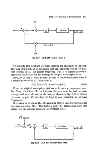
594. 578 6.4 Linear Modulation: Communications Context
We find that the resulting low-pass filter is identical to the unmodulated
case. Because the modulator simply shifted the message to a higher fre-
quency, we would expect the error variance to be the same. The error
variance follows easily.
Looking at the input to the system and recalling that
r(t) = [V2P cos wet] a(t) + n(t),
we see that the input to the loop is
(497)
r1(t) = [VP a(t) + n.(t)] + double frequency terms, (498)
where n.(t) is the original noise n(t) multiplied by V2/P cos wet.
Sn.(w) = ~ (499)
We see that this input is identical to that in Section 6.2. Thus the error
expression in (152) carries over directly.
gPn = ~; fo00 ln [1 + ~~~~] ~: (500)
for DSB-SC amplitude modulation. The curves in Figs. 6.17 and 6.19 for
the Butterworth and Gaussian spectra are directly applicable.
We should observe that the noise actually has the spectrum shown in Fig.
6.59 because there are elements operating at bandpass that the received
waveform passes through before being available for processing. Because
the filter in Fig. 6.58 is low-pass, the white noise approximation will be
valid as long as the spectrum is flat over the effective filter bandwidth.
6.4.2 DSB-AM: Demodulation with Delay
Now consider the same problem for the case in which unrealizable
filtering (or filtering with delay) is allowed. As a further simplification we
Fig. 6.59 Bandlimited noise with flat spectrum.

595. DSB-AM: Demodulation with Delay 579
assume that the message process is stationary. Thus T1 = oo and Ka(t, u) =
Ka(t - u). In this case, the easiest approach is to assume the Gaussian
model is valid and use the MAP estimation procedure developed in
Chapter 5. The MAP estimator equation is obtained from (6.3) and (6.4),
au(t) = J_"'"' ~0 Ka(t - u) c(u)[r(u) - c(u) a(u)] du, -00 < t < 00.
(501)
The subscript u emphasizes the estimator is unrealizable. We see that the
operation inside the integral is a convolution, which suggests the block
c(t)
c(t)
(a)
(b)
r(t) Sa(w) Ciu(t)
_..:...:...::_....;..~ X -------.-1 No !---.:...::.:.~-.;...
Sa(W) +2J>
(c)
Fig. 6.60 Demodulation with delay.

596. 580 6.4 Linear Modulation: Communications Context
diagram shown in Fig. 6.60a. Using an argument identical to that in
Section 6.4.1, we obtain the block diagram in Fig. 6.60b and finally in
Fig. 6.60c.
The optimum demodulator is simply a multiplication followed by an
optimum unrealizable filter.t The error expression follows easily:
g = Joo Sa(w)(N0/2P) dw.
u _oo Sa(w) + N0/2P 27T
(502)
This result, of course, is identical to that of the unmodulated process case.
As we have pointed out, this is because linear modulation is just a simple
spectrum shifting operation.
6.4.3 Amplitude Modulation: Generalized Carriers
In most conventional communication systems the carrier is a sine wave.
Many situations, however, develop when it is desirable to use a more
general waveform as a carrier. Some simple examples are the following:
1. Depending on the spectrum of the noise, we shall see that different
carriers will result in different demodulation errors. Thus in many cases a
sine wave carrier is inefficient. A particular case is that in which additive
noise is intentional jamming.
2. In communication nets with a large number of infrequent users we
may want to assign many systems in the same frequency band. An example
is a random access satellite communication system. By using different
wideband orthogonal carriers, this assignment can be accomplished.
3. We shall see in Part II that a wideband carrier will enable us to
combat randomly time-varying channels.
Many other cases arise in which it is useful to depart from sinusoidal
carriers. The modification of the work in Section 6.4.1 is obvious. Let
s(t, a(t)) = c(t) a(t). (503)
Looking at Fig. 6.60, we see that if
c2(t) a(t) = k[a(t) + a high frequency term] (504)
the succeeding steps are identical. If this is not true, the problem must be
re-examined.
As a second example of linear modulation we consider single-sideband
amplitude modulation.
t This particular result was first obtained in [46] (see also [45]).

597. Amplitude Modulation: Single-Sideband Suppressed-Carrier 581
6.4.4 Amplitude Modulation: Single-Sideband Suppressed-Caniert
In a single-sideband communication system we modulate the carrier
cos wet with the message a(t). In addition, we modulate a carrier sin wet
with a time function ti(t), which is linearly related to a(t). Thus the
transmitted signal is
s(t, a(t)) = VP [a(t) cos wet - ti(t) sin wet]. (505)
We have removed the v'2 so that the transmitted power is the same as
the DSB-AM case. Once again, the carrier is suppressed.
The function ti(t) is the Hilbert transform of a(t). It corresponds to the
output of a linear filter h(-r) when the input is a(t). The transfer function
of the filter is
{
-j,
HUw) = 0,
+j,
w > 0,
w = 0,
w < 0.
(506)
We can show (Problem 6.4.2) that the resulting signal has a spectrum
that is entirely above the carrier (Fig. 6.61).
To find the structure of the optimum demodulator and the resulting
performance we consider the case T1 = oo because it is somewhat easier.
From (505) we observe that SSB is a mixture of a no-memory term and a
memory term.
There are several easy ways to derive the estimator equation. We can
return to the derivation in Chapter 5 (5.25), modify the expression for
os(t, a(t))foAro and proceed from that point (see Problem 6.4.3). Alter-
natively, we can view it as a vector problem and jointly estimate a(t) and
ti(t) (see Problem 6.4.4). This equivalence is present because the trans-
mitted signal contains a(t) and ti(t) in a linear manner. Note that a state-
S.(w)
Fig. 6.61 SSB spectrum.
t We assume that the reader has heard of SSB. Suitable references are [47] to [49].

598. 582 6.4 Linear Modulation: Communications Context
variable approach is not useful because the filter that generates the Hilbert
transform (506) is not a finite-dimensional dynamic system.
We leave the derivation as an exercise and simply state the results.
Assuming that the noise is white with spectral height N0/2 and using
(5.160), we obtain the estimator equations
a(t) = ;.0J_..,.., v'P{cos WcZ Ra(t, z)- sin WcZ [J_ao.., h(z- y)Ra(t,y) dy]}
{r(z) - VP [a(z) cos w0 Z - b(z) sin w.z]} dz (507)
and
b(t) = ;.0J_"'"' VP {cos WcZ [J_"'"' h(t- y)Ra(Y, z) dy]- sin WcZ Ra(t,y)}
{r(z) - v'P [d(z) cos w0Z - b(z) sin w0z]} dz. (508)
These equations look complicated. However, drawing the block diagram
and using the definition of HUw) (506), we are led to the simple receiver
in Fig. 6.62 (see Problem 6.4.5 for details).
We can easily verify that n,(t) has a spectral height of N0f2. A com-
parison of Figs. 6.60 and 6.62 makes it clear that the mean-square per-
formance of SSB-SC and DSB-SC are identical. Thus we may use other
considerations such as bandwidth occupancy when selecting a system for
a particular application.
These two examples demonstrate the basic ideas involved in the estima-
tion of messages in the linear modulation systems used in conventional
communication systems.
Two other systems of interest are double-sideband and single-sideband
in which the carrier is not suppressed. The transmitted signal for the first
case was given in (488). The resulting receivers follow in a similar manner.
From the standpoint of estimation accuracy we would expect that
because part of the available power is devoted to transmitting a residual
carrier the estimation error would increase. This qualitative increase is
easy to demonstrate (see Problems 6.4.6, 6.4.7). We might ask why we
r(t) Unity gain
sideband
filter
a(t) + ns(t)
2
-..;p cos Wet
Fig. 6.62 SSB receiver.
Ba(w)
No 1----~
Sa(w) + 2p a(t)

599. Amplitude Modulation: Single-Sideband Suppressed-Carrier 583
would ever use a residual carrier. The answer, of course, lies in our model
of the communication link.
We have assumed that c(t), the modulation function (or carrier), is
exactly known at the receiver. In other words, we assume that the oscil-
lator at the receiver is synchronized in phase with the transmitter oscillator.
For this reason, the optimum receivers in Figs. 6.58 and 6.60 are frequently
referred to as synchronous demodulators. To implement such a demodu-
lator in actual practice the receiver must be supplied with the carrier in
some manner. In a simple method a pilot tune uniquely related to the
carrier is transmitted. The receiver uses the pilot tone to construct a
replica of c(t). As soon as we consider systems in which the carrier is
reconstructed from a signal sent from the transmitter, we encounter the
question of an imperfect copy of c(t). The imperfection occurs because
there is noise in the channel in which we transmit the pilot tone. Although
the details of reconstructing the carrier will develop more logically in
Chapter II.2, we can illustrate the effect of a phase error in an AM system
with a simple example.
Example. Let
r(t) = V2Pa(t)coswct + n(t). (509)
Assume that we are using the detector of Fig. 6.58 or 6.60. Instead of multiplying
by exactly c(t), however, we multiply by v'2P cos (wet + </>), where </> is phase angle
that is a random variable governed by some probability density Pf/J(</>). We assume
that </>is independent of n(t).
It follows directly that for a given value of t/> the effect of an imperfect phase
reference is equivalent to a signal power reduction:
Per = P cos2 </>. (510)
We can then find an expression for the mean-square error (either realizable or
nonrealizable) for the reduced power signal and average the result over Pf/J(</>). The
calculations are conceptually straightforward but tedious (see Problems 6.4.8 and
6.4.9).
We can see intuitively that if t/> is almost always small (say lt/>1 < 15°) the effect
will be negligible. In this case our model which assumes c(t) is known exactly is a
good approximation to the actual physical situation, and the results obtained from
this model will accurately predict the performance of the actual system. A number of
related questions arise:
1. Can we reconstruct the carrier without devoting any power to a pilot tone?
This question is discussed by Costas [SO]. We discuss it in the problem section of
Chapter 11.2.
2. If there is a random error in estimating c(t), is the receiver structure of Fig. 6.58
or 6.60 optimum? The answer in general is "no". Fortunately, it is not too far from
optimum in many practical cases.
3. Can we construct an optimum estimation theory that leads to practical receivers
for the general case of a random modulation matrix, that is,
r(t) = C(t) x(t) + n(t), (511)

600. 584 6.5 The Fundamental Role of the Optimum Linear Filter
where C(t) is random? We find that the practicality depends on the statistics of C(t).
(It turns out that the easiest place to answer this question is in the problem section
of Chapter 11.3.)
4. If synchronous detection is optimum, why is it not used more often? Here, the
answer is complexity. In Problem 6.4.10 we compute the performance of a DSB
residual-carrier system when a simple detector is used. For high-input SNR the
degradation is minor. Thus, whenever we have a single transmitter and many receivers
(e.g., commercial broadcasting), it is far easier to increase transmitter power than
receiver complexity. In military and space applications, however, it is frequently
easier to increase receiver complexity than transmitter power.
This completes our discussion of linear modulation systems. We now
comment briefly on some of the results obtained in this chapter.
6.5 THE FUNDAMENTAL ROLE OF THE OPTIMUM LINEAR FILTER
Because we have already summarized the results of the various sections
in detail it is not necessary to repeat the comments. Instead, we shall dis-
cuss briefly three distinct areas in which the techniques developed in this
chapter are important.
Linear Systems. We introduced the topic by demonstrating that for
linear modulation systems the MAP interval estimate of the message was
obtained by processing r(t) with a linear system. To consider point
estimates we resorted to an approach that we had not used before.
We required that the processor be a linear system and found the best
possible linear system. We saw that if we constrained the structure to
be linear then only the second moments of the processes were relevant.
This is an example of the type mentioned in Chapter 1 in which a partial
characterization is adequate because we employed a structure-oriented
approach. We then completed our development by showing that a linear
system was the best possible processor whenever the Gaussian assumption
was valid. Thus all of our results in this chapter play a double role. They
are the best processors under the Gaussian assumptions for the classes of
criteria assumed and they are the best linear processors for any random
process.
The techniques of this chapter play a fundamental role in two other
areas.
Nonlinear Systems. In Chapter 11.2 we shall develop optimum receivers
for nonlinear modulation systems. As we would expect, these receivers are
nonlinear systems. We shall find that the optimum linear filters we have
derived in this chapter appear as components of the over-all nonlinear
system. We shall also see that the model of the system with respect to its

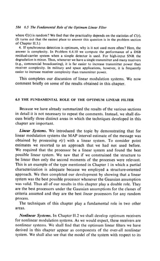
601. Comments 585
effect on the message is linear in many cases. In these cases the results in
this chapter will be directly applicable. Finally, as we showed in Chapter 5
the demodulation error in a nonlinear system can be bounded by the error
in some related linear system.
Detection ofRandom Processes. In Chapter II.3 were turn to the detection
and estimation problem in the context of a more general model. We shall
find that the linear filters we have discussed are components of the
optimum detector (or estimator).
We shall demonstrate why the presence of an optimum linear filter
should be expected in these two areas. When our study is completed the
fundamental importance of optimum linear filters in many diverse con-
texts will be clear.
6.6 COMMENTS
It is worthwhile to comment on some related issues.
1. In Section 6.2.4 we saw that for stationary processes in white noise
the realizable mean-square error was related to Shannon's mutual informa-
tion. For the nonstationary, finite-interval case a similar relation may also
be derived
gP = 2 N08l(T:r(t), a(t)).
2 BT
(512)
2. The discussion with respect to state-variable filters considered only
the continuous-time case. We can easily modify the approach to include
discrete-time systems. (The discrete system results were derived in Problem
2.6.15 of Chapter 2 by using a sequential estimation approach.)
3. Occasionally a problem is presented in which the input has a transient
nonrandom component and a stationary random component. We may
want to minimize the mean-square error caused by the random input
while constraining the squared error due to transient component. This is a
straightforward modification of the techniques discussed (e.g., [51]).
4. In Chapter 3 we discussed the eigenfunctions and eigenvalues of the
integral equation,
, cp(t) = JT' Ky(t, u) cp(u) du, T; s t s T1
. (513)
Tt
For rational spectra we obtained solutions by finding the associated
differential equation, solving it, and using the integral equation to evaluate
the boundary conditions. From our discussion in Section 6.3 we anticipate
that a computationally 'more efficient method could be found by using

602. 586 6.7 Problems
state-variable techniques. These techniques are developed in [52] and [54]
(see also Problems 6.6.1-6.6.4) The specific results developed are:
(a) A solution technique for homogeneous Fredholm equations using
state-variable methods. This technique enables us to find the eigenvalues
and eigenfunctions of scalar and vector random processes in an efficient
manner.
(b) Asolutiontechnique for nonhomogeneous Fredholm equations using
state-variable methods. This technique enables us to find the function
g(t) that appears in optimum detector for the colored noise problem. It is
also the key to the optimum signal design problem.
(c) A solution of the optimum unrealizable filter problem using state-
variable techniques. This enables us to achieve the best possible per-
formance using a given amount of input data.
The importance of these results should not be underestimated because
they lead to solutions that can be evaluated easily with numerical techn-
niques. We develop these techniques in greater detail in Part II and use
them to solve various problems.
5. In Chapter 4 we discussed whitening filters for the problem of detect-
ing signals in colored noise. In the initial discussion we did not require
realizability. When we examined the infinite interval stationary process
case (p. 312), we determined that a realizable filter could be found and one
component interpreted as an optimum realizable estimate of the colored
noise. A similar result can be derived for the finite interval nonstationary
case (see Problem 6.6.5). This enables us to use state-variable techniques
to find the whitening filter. This result will also be valuable in Chapter
11.3.
6.7 PROBLEMS
P6.1 Properties of Linear Processors
Problem 6.1.1. Let
r(t) = a(t) + n(t),
where a(t) and n(t) are uncorrelated Gaussian zero-mean processes with covariance
functions Ka(t, u) and Kn(t, u), respectively. Find Pa<t1>i'<t>;Tp;;t s r 1(A lr(t) :T, $ t $ T1).
Problem 6.1.2. Consider the model in Fig. 6.3.
1. Derive Property 3V (51).
2. Specialize (51) to the case in which d(t) = x(t).
Problem 6.1.3.
Consider the vector model in Fig. 6.3.
Prove that

603. Properties ofLinear Processors 587
Comment. Problems 6.1.4 to 6.1.9 illustrate cases in which the observation is a
finite set of random variables. In addition, the observation noise is zero. They
illustrate the simplicity that (29) leads to in linear estimation problems.
Problem 6.1.4. Consider a simple prediction problem. We observe a(t) at a single
time. The desired signal is
d(t) = a(t + a),
where a is a positive constant. Assume that
E[a(t)] = 0,
E[a(t) a(u)] = K.(t - u) !l K.(,.),
1. Find the best linear MMSE estimate of d(t).
2. What is the mean-square error?
3. Specialize to the case K.(,.) = e-kl•l.
4. Show that, for the correlation function in part 3, the MMSE estimate would
not change if the entire past were available.
5. Is this true for any other correlation function? Justify your answer.
Problem 6.1.5. Consider the following interpolation problem. You are given the
values a(O) and a(T):
E[a(t)] = 0,
E[a(t)a(u)] = K.(t - u),
l. Find the MMSE estimate of a(t).
2. What is the resulting mean-square error?
3. Evaluate for t = T/2.
-oo < t < oo,
-00 < t, u < 00,
4. Consider the special case, Ka(T) = e-kl•l, and evaluate the processor constants
Problem 6.1.6 [55]. We observe a(t) and d(t). Let d(t) = a(t + a), where a is a positive
constant.
l. Find the MMSE linear estimate of d(t).
2. State the conditions on K.(T) for your answer to be meaningful.
3. Check for small a.
Problem 6.1.7 [55]. We observe a(O) and a(t). Let
d(t) = L'a(u) du.
l. Find the MMSE linear estimate of d(t).
2. Check your result for t « 1.
Problem 6.1.8. Generalize the preceding model to n + l observations; a(O), a(t).
a(2t) · · · a(nt).
J.nt
d(t) = 0
a(u) du.
1. Find the equations which specify the optimum linear processor.
2. Find an explicit solution for nt « I.

604. 588 6.7 Problems
Problem 6.1.9. [55]. We want to reconstruct a(t) from an infinite number of samples;
a(nT), n = · · · -1, 0, + 1, ... , using a MMSE linear estimate:
00
a(t) = L Cn(t) a(nT).
n=- oo
I. Find an expression that the coefficients c.(t) must satisfy.
2. Consider the special case in which
s.(w) = 0
7T
lwl > T'
Evaluate the coefficients.
3. Prove that the resulting mean-square error is zero. (Observe that this proves the
sampling theorem for random processes.)
Problem 6.1.10. In (29) we saw that
E[e0 (t) r(u)] = 0,
1. In our derivation we assumed h0 (t, u) was continuous and defined h,(t, T,) and
ho(t, T1) by the continuity requirement. Assume r(u) contains a white noise com-
ponent. Prove
E[e0 (t)r(T,)] #- 0,
E[e0 (t)r(T1)] #- 0.
2. Now remove the continuity assumption on ho(t, u) and assume r(u) contains a
white noise component. Find an equation specifying an ho(t, u), such that
E[e0 (t)r(u)] = 0,
Are the mean-square errors for the filters in parts I and 2 the same? Why?
3. Discuss the implications of removing the white noise component from r(u).
Will ho(t, u) be continuous? Do we use strict or nonstrict inequalities in the integral
equation?
P6.2 Stationary Processes, Infinite Past, (Wiener Filters)
REALIZABLE AND UNREALIZABLE FILTERING
Problem 6.2.1. We have restricted our attention to rational spectra. We write the
spectrum as
(w- n,)(w- n2)· • ·(w- liN)
S,(w) = C d d d '
(w - ,)(w - 2)· · ·(w - M)
where Nand Mare even. We assume that S,(w) is integrable on the real line. Prove
the following statements:
1. S,(w) = S,*(w).
2. c is real.
3. Alln,'s and d.'s with nonzero imaginary parts occur in conjugate pairs.
4. S,(w) 2: 0.
5. Any real roots of numerator occur with even multiplicity.
6. No root of the denominator can be real.
7. N< M.
Verify that these res~lts imply all the properties indicated in Fig. 6.7.

605. Stationary Processes, Infinite Past, (Wiener Filters) 589
Problem 6.2.2. Let
r(u) = a(u) + n(u), -oo < u ::5 t.
The waveforms a(u) and n(u) are sample functions from uncorrelated zero-mean
processes with spectra
and
respectively.
I. The desired signal is a(t ). Find the realizable linear filter which minimizes the
mean-square error.
2. What is the resulting mean-square error?
3. Repeat parts I and 2 for the case in which the filter may be unrealizable and
compare the resulting mean-square errors.
Problem 6.2.3. Consider the model in Problem 6.2.2. Assume that
1. Repeat Problem 6.2.2.
2. Verify that your answers reduce to those in Problem 6.2.2 when No = 0 and to
those in the text when N2 = 0.
Problem 6.2.4. Let
r(u) = a(u) + n(u), -00 < u ::5 t.
The functions a(u) and n(u) are sample functions from independent zero-mean
Gaussian random processes.
2kaa2
s.(w) = ----.----k.'
w +
S (w) = 2can2
•
n w2 + C2
We want to find the MMSE point estimate of a(t).
I. Set up an expression for the optimum processor.
2. Find an explicit expression for the special case
O'n2 = O'a2,
c = 2k.
3. Look at your answer in (2) and check to see if it is intuitively correct.
Problem 6.2.5. Consider the model in Problem 6.2.4. Now let
S ( ) _ No 2can2 •
n w - 2 + w• + c2
1. Find the optimum realizable linear filter (MMSE).
2. Find an expression for tPn·
3. Verify that the result in (1) reduces to the result in Problem 6.2.4 when N 0 = 0
and to the result in the text when an2 = 0.

606. 590 6.7 Problems
Problem 6.2.6. Let
r(u) = a(u) + w(u),
The processes are uncorrelated with spectra
-00 < u :$; t.
and
2V2Pfk
S.(w) = I + (w•jk•)•
Sw(w) = ~0•
The desired signal is a(t). Find the optimum realizable linear filter (MMSE).
Problem 6.2.7. The message a(t) is passed through a linear network before trans-
mission as shown in Fig. P6.1. The output y(t) is corrupted by uncorrelated white
noise (No/2). The message spectrum is S.(w).
2kaa2
s.(w) = w2 + k..
1. A minimum mean-square error realizable estimate of a(t) is desired. Find the
optimum linear filter.
2. Find tPn as a function of a and A ~ 4aa2/kNo.
3. Find the value of a that minimizes tPn·
4. How do the results change if the zero in the prefilter is at +k instead of - k.
w(t) (~o)
Prefilter
Fig. P6.1
Pure Prediction. The next four problems deal with pure prediction. The model is
r(u) = a(u), -00 < u :$; t,
and
d(t) = a(t + a),
where a ~ 0. We see that there is no noise in the received waveform. The object is
to predict a(t ).
Problem 6.2.8. Let
2k
s.(w) = w• + k ..
1. Find the optimum (MMSE) realizable filter.
2. Find the normalized prediction error g~•.
Problem 6.2.9. Let
Sa(w) = (l + w•)2
Repeat Problem 6.2.8.

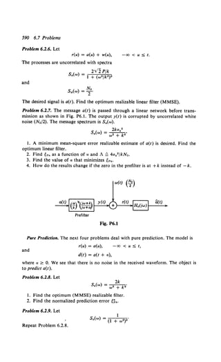
607. Stationary Processes, Infinite Past, (Wiener Filters) 591
Problem 6.2.10. Let
Repeat Problem 6.2.8.
Problem 6.2.11.
1 + w2
Sa(w) = l + "'4 •
1. The received signal is a(u), -oo < u :5 t. The desired signal is
d(t) = a(t + a),
Find H.(jw) to minimize the mean-square error
a> 0.
E{[d(t) - d(t)]2},
where
d(t) = f.,h.(t - u) a(u) du.
The spectrum of a(t) is
wherek, ¥- k1 ; i ¥-j fori= l, ... ,n,j = l, ... ,n.
2. Now assume that the received signal is a(u), T, :5 u :5 t, where T, is a finite
number. Find h.(t, T) to minimize the mean-square error.
d(t) = f' h.(t, u) a(u) du.
Jr,
3. Do your answers to parts 1 and 2 enable you to make any general statements
about pure prediction problems in which the message spectrum has no zeros?
Problem 6.2.12. The message is generated as shown in Fig. P6.2, where u(t) is a white
noise process (unity spectral height) and a., i = 1, 2, and A., i = 1, 2, are known
positive constants. The additive white noise w(t)(No/2) is uncorrelated with u(t).
I. Find an expression for the linear filters whose outputs are the MMSE realizable
estimates of x,(t), i = 1, 2.
2. Prove that
3. Assume that
Prove that
u(t)
2
a<t> = L: x.<t>.
t=l
2
d(t) = 2: d, x,(t).
t~l
Fig. P6.2
r(t)

608. 592 6.7 Problems
Problem 6.2.13. Let
r(u) = a(u) + n(u), -00 < u ::; t,
where a(u) and n(u) are uncorrelated random processes with spectra
w2
Sa(w) =-4 - -
1,
w +
1
s.(w) =--·
w2 + E2
The desired signal is a(t). Find the optimum (MMSE) linear filter and the resulting
error for the limiting case in which •->- 0. Sketch the magnitude and phase of H 0 (jw).
Problem 6.2.14. The received waveform r(u) is
r(u) = a(u) + w(u), -oo < u :S t,
where a(u) and w(u) are uncorrelated random processes with spectra
Let
2ka.2
s.(w) = --r--k2'
w +
s.(w) = ~0•
rt+a
d(t) Q_ J, a(u) du, a> 0.
1. Find the optimum (MMSE) linear filter for estimating d(t).
2. Find g~.
Problem 6.2.15(continuation). Consider the same model as Problem 6.2.14. Repeat
that problem for the following desired signals:
1 r~
I. d(t) =;; Jt-• a(u) du, a> 0.
I it+P
2. d(t) = ~ a(u) du,
f-.1 a t+a
a> O,{J > O,{J ~a.
What happens as(~ - a)-+ 0?
+1
3. d(t) = 2 kn a(t - na), a> 0.
n= -1
Problem 6.2.16. Consider the model in Fig. P6.3. The function u(t) is a sample
function from a white process (unity spectral height). Find the MMSE realizable linear
estimates, .i1(t) and .i2 (t). Compute the mean-square errors and the cross correlation
between the errors (T, = -oo).
w(t) (~o)
u(t) r(t)
Fig. P6.3

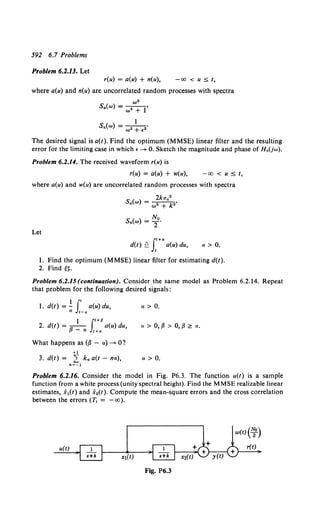
609. Stationary Processes, Infinite Past, (Wiener Filters) 593
~­
~
Fig. P6.4
r(t)
Problem 6.2.17. Consider the communication problem in Fig. P6.4. The message a(t)
is a sample function from a stationary, zero-mean Gaussian process with unity
variance. The channel k1(T) is a linear, time-invariant, not necessarily realizable system.
The additive noise n(t) is a sample function from a zero-mean white Gaussian process
(N0 /2).
I. We process r(t) with the optimum unrealizable linear filter to find ii(t). Assuming
S:ro IK1(jw)i 2(dwj27T) = 1, find the k1(T) that minimizes the minimum mean-square
error.
2. Sketch for
2k
Sa(w) = w• + p"
CLOSED FORM ERROR EXPRESSIONS
Problem 6.2.18. We want to integrate
No fro dw [ 2c./No ]
(p = 2 _ro 27T In l + 1 + (w/k)2 " •
1. Do this by letting y = 2cnfN 0 • Differentiate with respect to y and then integrate
with respect to w. Integrate the result from 0 to y.
2. Discuss the conditions under which this technique is valid.
Problem 6.2.19. Evaluate
Comment. In the next seven problems we develop closed-form error expressions
for some interesting cases. In most of these problems the solutions are difficult. In all
problems
r(u) = a(u) + n(u), -00 < u ::5 t,
where a(u) and n(u) are uncorrelated. The desired signal is a(t) and optimum (MMSE)
linear filtering is used. The optimum realizable linear filter is H.(jw) and
G.(jw) Q 1 - H0 (jw).
Most of the results were obtained in [4].
Problem 6.2.20. Let
Show that
Naa•
S(w)=--·
n w2 + a•
H0 (jw) = 1 - k [Sn(w)] + •
[Sa(w) + s.(wW

610. 594 6.7 Problems
where
[ 2 f"' S,.(w) dw]
k = exp Noa Jo S,.(w) ln S,.(w) + S,.(w) 2w .
Problem 6.2.21. Show that if lim S,.(w)-- 0 then
..~ ..
~P = 2 r{S,.(w) - JG.(jw)J 2[S,.(w) + S,.(w)]} ~:·
Use this result and that of the preceding problem to show that for one-pole noise
~P = Nt(1 - k").
Problem 6.2.22. Consider the case
Show that
IG (. )J" S,.(w) + K
0 }W = S,.(w) + Siw)'
where
f"' In [ S,.(w) + K ] dw = 0
Jo S,.(w) + S,.(w)
determines K.
Problem 6.2.23. Show that when S,.(w) is a polynomial
~P = _! f"' dw{S,.(w) - JG.(jw)J2 [S,.(w) + S,.(w)] + S,.(w) In JG.(jw)J 2}•
., Jo
Problem 6.2.24. As pointed out in the text, we can double the size of the class
of problems for which these results apply by a simple observation. Figure P6.5a
represents a typical system in which the message is filtered before transmission.
a(t)
a(t)
(a)
n(e)
N.
[Sn(w) =2flo2 w2)
(b)
Fig. P6.5
r(t)

611. Stationary Processes, Infinite Past, (Wiener Filters) 595
Clearly the mean-square error in this system is identical to the error in the system
in Fig. P6.Sb. Using Problem 6.2.23, verify that
t - 1 f"' [No 2 [No 2 x] Now•! I . i•]
!OP - -;;: Jo 2132 "' - 2132 w + + 2132 n G.(jw) dw
1 f"' [ Now2 ( Sn{w) + K )]
= :;;: Jo K - 2f32 In S.,(w) + Sn(w) dw.
Problem 6.2.25 (conti1111ation) [39]. Using the model of Problem 6.2.24, show that
eP = ~0 [/(0))3 + F(O),
where
/(0) =I"' ln [t + 2f32f.,(w)] dw
-ao w No 27T
and
F(O) = f"' w• No2ln [1 + 2/3"!.,(w)] dw.
-.. 2p w No 27T
Problem 6.2.26 [20]. Extend the results in Problem 6.2.20 to the case
( ) No N1a2
5• "' = T + w 2 + a2
FEEDBACK REALIZATIONS
Problem 6.2.27. Verify that the optimum loop filter is of the form indicated in Fig.
6.21b. Denote the numerator by F(s).
1. Show that
F(s) = [~ B(s) B(-s) + P(s) P(- s)] + - P(s),
where B(s) and P(s) are defined in Fig. 6.2la.
2. Show that F(s) is exactly one degree less than P(s).
Problem 6.2.28. Prove
t No 1. No
~P =-2 1m sG1.(s) = -2 fn-1·
.~ ..
where G,.(s) is the optimum loop filter andfn- 1 is defined in Fig. 6.2lb.
Problem 6.2.29. In this problem we construct a realizable whitening filter. In Chapter 4
we saw that a conceptual unrealizable whitening filter may readily be obtained in
terms of a Karhunen-Loeve expansion. Let
r(u) = nc(u) + w(u), -oo < u :S t,
where nc(u) has a rational spectrum and w(u) is an uncorrelated white noise process.
Denote the optimum (MMSE) realizable linear filter for estimating nc(t) as H.(jw).
l. Prove that 1 - H.(jw) is a realizable whitening filter. Draw a feedback realiza-
tion of the whitening filter.

612. 596 6.7 Problems
Hint. Recall the feedback structure of the optimum filter (173).
2. Find the inverse filter for I - H 0 (jw). Draw a feedback realization of the inverse
filter.
Problem 6.2.30 (continuation). What are the necessary and sufficient conditions for
the inverse of the whitening filter found in Problem 6.2.29 to be stable?
GENERALIZATIONS
Problem 6.2.31. Consider the simple unrealizable filter problem in which
r(u) = a(u) + n(u), -co < u <co
and
d(t) = a(t).
Assume that we design the optimum unrealizable filter H 0 .(jw) using the spectrum
Sa(w) and Sn(w). In practice the noise spectrum is
Snp(w) = S•.(w) + Sn,(w).
1. Show that the mean-square error using HouUw) is
I"' dw
~up = ~uo + _"' IHou(jw)l2 Sne(w) 2,;
where up denotes unrealizable mean-square error in practice and uo denotes un-
realizable mean-square error in the optimum filter when the design assumptions are
exact.
2. Show that the change in error is
3. Consider the case
No
Sne(w) = < T'
The message spectrum is flat and bandlimited. Show that
•A
<l~u = (1 + A)2'
where A is the signal-to-noise ratio in the message bandwidth.
Problem 6.2.32. Derive an expression for the change in the mean-square error in an
optimum unrealizable filter when the actual message spectrum is different from the
design message spectrum.
Problem 6.2.33. Repeat Problem 6.2.32 for an optimum realizable filter and white
noise.
Problem 6.2.34. Prove that the system in Figs. 6.23b is the optimum realizable filter
for estimating a(t).

613. Stationary Processes, Infinite Past, (Wiener Filters) 597
Problem 6.2.35. Derive (181) and (183) for arbitrary K"(jw).
Problem 6.2.36. The mean-square error using an optimum unrealizable filter is given
by(183):
g _ Joo Sa(w) Sn(w) dw
uo - _ 00 S 0 (w) Sr(w) + Sn(w) 2,/
where s,(w) ~ IK,(jw)l2 •
1. Consider the following problem. Constrain the transmitted power
J
oo dw
P = _ oo Sa(w) S,(w) 2,;
Find an expression for S1(w) that minimizes the mean-square error.
2. Evaluate the resulting mean-square error.
Problem 6.2.37. Let
r(u) = a(u) + n(u),
where a(u) and n(u) are uncorrelated. Let
1
Sa(w) = -
1- -
2 •
+w
The desired signal is d(t) = (djdt) a(t).
1. Find H 0 (jw).
-00 < u :::; t,
2. Discuss the behavior of Ho(jw) and gP as •-+ 0. Why is the answer misleading?
Problem 6.2.38. Repeat Problem 6.2.37 for the case
What is the important difference between the message random processes in the two
problems? Verify that differentiation and optimum realizable filtering do not commute.
Problem 6.2.39. Let
a(u) = cos (2rrfu + </>),
where 4> and fare independent variables:
and
1
p~(<fo) = 27T'
Pr(X) = 0,
1. Describe the resulting ensemble.
2. Prove that Sa(/) = Pr(lfi)/4.
x:::; o.
-00 < u :::; t,
3. Choose a p1(X) to make a(t) a deterministic process (seep. 512). Demonstrate a
linear predictor whose mean-square error is zero.
4. Choose a p 1(X) to make a(t) a nondeterministic process. Show that you can
predict a(t) with zero mean-square error by using a nonlinear predictor.

614. 598 6.7 Problems
Problem 6.2.40. Let
g+('r) = 3'- 1 [G+(jw)).
Prove that the MMSE error for pure prediction is
t~ = J:[g+(T)]2 dT.
Problem 6.2.41 [1]. Consider the message spectrum
1. Show that
+ Tn- 1exp(- Tv'ii)
g (T) = n-nl•(n- 1)! .
2. Show that (for large n)
['f.~ J:2
1
.. exp [ -z(t- n;nTJdt.
3. Use part 2 to show that for any e2 and a we can make
by increasing n sufficiently. Explain why this result is true.
Problem 6.1.41. The message a(t) is a zero-mean process observed in the absence of
noise. The desired signal d(t) = a(t + a), a > 0.
l. Assume
1
Ka(T) =.---k
..
'T +
Find d(t) by using a(t) and its derivatives. What is the mean-square error for a < k?
2. Assume
Show that
"' [dn ]an
d(t + a) = 2 -d
n a(t) I'
n~o t n.
and that the mean-square error is zero for all a,
Problem 6.1.43. Consider a simple diversity system,
r1(t) = a(t) + n1(t),
r.(t) = a(t) + n2(t),
where a(t), n1(t), and n2(t) are independent zero-mean, stationary Gaussian processes
with finite variances. We wish to process r1 (t) and r2 (t), as shown in Fig. P6.6. The
spectra Sn1 (w) and Sn2 (w) are known; S.(w), however, is unknown. We require that
the message a(t) be undistorted. In other words, if n1(t) and n2(t) are zero, the output
will be exactly a(t).
l. What condition•does this impose on H 1(jw) and H.(jw)?
2. We want to choose H 1(jw) to minimize E[nc2(t)], subject to the constraint that

615. Finite-time, Nonstationary Processes (Kalman-Bucy Filters) 599
rt(t)
a(t) + nc(t)
+)--.....;...;.__.;;..;_;..._~
Fig. P6.6
a(t) be reproduced exactly in the absence of input noise. The filters must be realizable
and may operate on the infinite past. Find an expression for H,0 (jw) and H20 (jw) in
terms of the given quantities.
3. Prove that the d(t) obtained in part 2 is an unbiased, efficient estimate of the
sample function a(t). [Therefore a(t) = dm1(t).]
Problem 6.2.44. Generalize the result in Problem 6.2.43 to the n-input problem.
Prove that any n-dimensional distortionless filter problem may be recast as an
(n - I)-dimensional Wiener filter problem.
P6.3 Finite-time, Nonstationary Processes (Kalman-Bucy filters)
STATE-VARIABLE REPRESENTATIONS
Problem 6.3.1. Consider the differential equation
y<•>(t) + Pn-lY<n-l>(t) + •••+ PoY(t) = b•. ,u<•-l>(t) + ••·+ bou(t).
Extend Canonical Realization 1 on p. 522 to include this case. The desired F is
0 : 1 0 1
.~r=~)-~;~-------=;::;
Draw an analog computer realization and find the G matrix.
Problem 6.3.2. Consider the differential equation in Problem 6.3.1. Derive Canonical
Realization 3 (see p. 526) for the case of repeated roots.
Problem 6.3.3 [27]. Consider the differential equation
y<•>(t) + Pn-IY<n-I>(t) + ···+ PoY(t) = b._,u<•-'>(t) + ···+ bou(t).
1. Show that the system in Fig. P6.7 is a correct analog computer realization.
2. Write the vector differential equation that describes the system.
Problem 6.3.4. Draw an analog computer realization for the following systems:
1. y(t) + 3y(t) + 4y(t) = u(t) + u(t),
2. ji1(t) + 3.)(t) + 2y2(t) = u,(t) + 2u2(t) + 2u2(t),
ji2(t) + 4;(t) + 3y2(t) = 3u2(1) + u,(t).
Write the associated vector differential equation.

616. 600 6.7 Problems
y(t)
Fig. P6.7
Problem 6.3.5 [27]. Find the transfer function matrix and draw the transfer function
diagram for the systems described below. Comment on the number of integrators
required.
1. .h(t) + 3J(t) + 2y,{t) = u,(t) + 2u,(t) + u.(t) + u.(t),
y.(t) + 2y.(t) = -u,(t) - 2u,(t) + u2 (t).
2. y1(t) + y1 (t) = u1 (t) + 2u2 (t),
.Y.(t) + 3.Ji2(t) + 2y,(t) = u.(t) + u.(t) - u,(t).
3. ji,(t) + 2y.(t) + y,(t) = u,(t) + u,(t) + u.(t),
Y,(t) + y,(t) + y.(t) = u.(t) + u,(t).
4. ji,(t) + 3;(t) + 2y,(t) = 3u,(t) + 4u.(t) + su.(t),
.Y2(t) + 3y2(t) - 4y,(t) - y,(t) = u,(t) + 2u2(t) + 2u2(t).
Problem 6.3.6 [27]. Find the vector differential equations for the following systems,
using the partial fraction technique.
1. ji(t) + 3y(t) + 2y(t) = u(t),
2. 'ji(t) + 4ji(t) + Sy(t) + 2y(t) = u(t),
3. 'ji(t) + 4ji(t) + 6y(t) + 4y(t) = u(t),
4. ji1(1) - 10y2(t) + y1(t) = u1(t),
y2 (t) + 6y2(t) = u2 (t).
Problem 6.3.7. Compute eFt for the following matrices:
1. F=
[~ l
2. F= [_~ !l
[-2 -~]·
3. F=
-4

617. Finite-time, Nonstationary Processes (Kalman-Bucy Filters)
Problem 6.3.8. Compute eF1 for the following matrices:
~
1
~·
1. F= 0
0
~
1
~·
2. F= 0
0 -1
3. F=
u0
l
-11 -
Problem 6.3.9. Given the system with state representation as follows,
i(t) = F x(t) + G u(t),
y(t) = C x(t),
x(O) = 0.
601
Let U(s) and Y(s) denote the Laplace transform of u(t) and y(t), respectively. We
found that the transfer function was
H(s) = Y(s) = C clt(s)G
U(s)
= C(sl - F)- 1G.
Show that the poles of H(s) are the eigenvalues of the matrix F.
Problem 6.3.10. Consider the circuit shown in Fig. P6.8. The source is turned on
at t = 0. The current i(O-) and the voltage across the capacitor Vc(O-) are both zero.
The observed quantity is the voltage across R.
1. Write the vector differential equations that describe the system and an equation
that describes the observation process.
2. Draw an analog computer realization of the circuit.
c L
+
t
R y(t)
t
Fig. P6.8
Problem 6.3.11. Consider the control system shown in Fig. P6.9. The output of the
system is a(t). The two inputs, b(t) and n(t), are sample functions from zero-mean,
uncorrelated, stationary random processes. Their spectra are
2a02 k
s.(w) = w• + k"

618. 602 6.7 Problems
b(t)
+
and
n(t)
Fig. P6.9
No
Sn(w) = T'
a(t)
Write the vector differential equation that describes a mathematically equivalent
system whose input is a vector white noise u(t) and whose output is a(t).
Problem 6.3.12. Consider the discrete multipath model shown in Fig. P6.10. The
time delays are assumed known. The channel multipliers are independent, zero-mean
processes with spectra
for j = 1,2,3.
The additive white noise is uncorrelated and has spectral height No/2. The input
signal s(t) is a known waveform.
1. Write the state and observation equations for the process.
2. Indicate how this would be modified if the channel gains were correlated.
Problem 6.3.13. In the text we considered in detail state representations for time
invariant systems.
Consider the time varying system
ji(t) + P1(t) y(t) + Po(t) y(t) = b1(t) li(t) + bo(t) u(t).
s(t)
Fig. P6.10

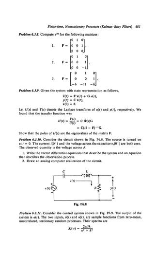
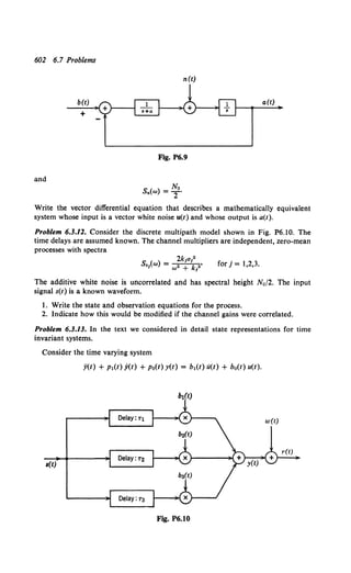
619. Finite-time, Nonstationary Processes (Kalman-Bucy Filters) 603
Show that this system has a state representation of the same form as that in Example 2.
t}_ x(t) = [ 0 1 ]x(t) + [h1
(t)] u(t),
dt -p0(t) -p1(t) h2(t)
y(t) = [1 0] x(t) = x1(t),
where h1(t) and h2(t) are functions that you must find.
Problem 6.3.14 [27]. Given the system defined by the time-varying differential equation
n-1 n
y<•>(t) + L Pn-k(t) y<k>(t) = L bn-k(t) lfk>(t),
k=O k=O
Show that this system has the state equations
where
.X1(t)
.X2(t)
.x.(t)
0
0
1
0
-p. -Pn-1
0
1
y(t) = x1(t) + go(t) u(t),
go(t) = bo(t),
0
0
x1(t)
X2(t)
- P1 Xn(t)
gl(t)
g2(t)
+ u(t)
g.(t)
I - 1 I- r (n + m - i)
g,(t) = b,(t)- '~ m~O n- i P·-r-m(t)g~m>(t).
Problem 6.3.15. Demonstrate that the following is a solution to (273).
Ax(t) = cl>(t, to)[AxCto) + Lcl>(to, T)G(T) Q(T) GT(T)ci>T(t0, T) dT]c~>T(t, 10),
where cl>(t, t0) is the fundamental transition matrix; that is,
d
di''l>(t, to) = F(t) cl>(t, t 0),
cl>(to, to) = I.
Demonstrate that this solution is unique.
Problem 6.3.16. Evaluate Ky(t, T) in terms of Kx(t, t) and cl>(t, T), where
:i(t) = F(t) x(t) + G(t) u(t),
y(t) = C(t) x(t),
E[u(t) uT(T)] = Q S(t - T).
Problem 6.3.17. Consider the first-order system defined by
d~~) = - k(t) x(t) + g(t) u(t).
y(t) = x(t).

620. 604 6.7 Problems
1. Determine a general expression for the transition matrix for this system.
2. What is h(t, T) for this system?
3. Evaluate h(t, T) for
k(t) = k(1 + m sin (w0t)),
g(t) = 1.
4. Does this technique generalize to vector equations?
Problem 6.3.18. Show that for constant parameter systems the steady-state variance
of the unobserved process is given by
where
lim Kx(t, t) = fo"' e+F•GQGTeFTr d'T,
t... GO J1
i(t) = Fx(t) + Gu(t),
E[u(t) uT(T)] = Q ll(t - T),
or, equivalently,
Problem 6.3.19. Prove that the condition in (317) is necessary when R(t) is positive-
definite.
Problem 6.3.20. In this problem we incorporate the effect of nonzero means into our
estimation procedure. The equations describing the model are (302)-(306).
1. Assume that x(T.) is a Gaussian random vector
E[x(T.)] Q m(T,) of 0,
and
E{[x(T,) - m(1j)][xT(T,) - mT(T,)]} = Kx(T;, 7;).
It is statistically independent of u(t) and w(t). Find the vector differential equations
that specify the MMSE estimate x(t), t :2: T,.
2. Assume that m(T,) = 0. Remove the zero-mean assumption on u(t),
E[u(t)] = mu(t),
and
E{[u(t)- mu(t))[uT(T) - muT(T)]} = Q(t)ll(t - T).
Find the vector differential equations that specify i(t).
Problem 6.3.21. Consider Example 1 on p. 546. Use Property 16 to derive (351).
Remember that when using the Laplace transform technique the contour must be
taken to the right of all the poles.
Problem 6.3.22. Consider the second-order system illustrated in Fig. P6.11, where
E[u(t) u(T)] = 2Pab(a + b) ll(t- T),
No )
E[w(t) w(T)] = T ll(t - T.
(a, b are possibly complex conjugates.) The state variables are
Xt(t) = y(t),
x2(t) = y(t).

621. Finite-time, Nonstationary Processes (Kalman-Bucy Filters) 605
w(t)
u(t) r(t)
Fig. P6.11
1. Write the state equation and the output equation for the system.
2. For this state representation determine the steady state variance matrix Ax of
the unobserved process. In other words, find
Ax = lim E[x(t) xT(t)],
t~.,
where x(t) is the state vector of the system.
3. Find the transition matrix T(t, T1) for the equation,
GQGT]
T(t, T,),
-FT
[text (336)]
by using Laplace transform techniques. (Depending on the values of a, b, q, and
No/2, the exponentials involved will be real, complex, or both.)
4. Find ;p(t) when the initial condition is
l;p(T,) = Ax.
Comment. Although we have an analytic means of determining ;p(t) for a system
of any order, this problem illustrates that numerical means are more appropriate.
Problem 6.3.23. Because of its time-invariant nature, the optimal linear filter, as
determined by Wiener spectral factorization techniques, will lead to a nonoptimal
estimate when a finite observation interval is involved. The purpose of this problem
is to determine how much we degrade our estimate by using a Wiener filter when the
observation interval is finite. Consider the first order system.
where
x(t) = -kx(t) + u(t),
r(t) = x(t) + w(t),
E[u(t) u(-r)] = 2kP 3(t - -r),
No
E[w(t) w(-r)] = T S(t - -r),
E[x(O)] = 0,
E[x2 (0)] = Po.
T1 = 0.
I. What is the variance of error obtained by using Kalman-Bucy filtering?
2. Show that the steady-state filter (i.e., the Wiener filter) is given by
. 4kP/No
H.(Jw) = (k + y)(jw + y)'
where y = k(l + 4PjkN0)Y•. Denote the output of the Wiener filter as Xw0(t).

622. 606 6.7 Problems
3. Show that a state representation for the Wiener filter is
• ( A ( ) 4Pk (
:fw0 t) = -y Xw0 t + No(k + y)' t),
where
Xw0 (0) = 0.
4. Show that the error for this system is
iw0(t) = - y Ew0(t) - u(t) + No(~P: y) w(t),
Ew0(0) = -x(O).
5. Define
Show that
and verify that
t 4kPy
~w.(t) = - z,..gw.(t) + 'Y + k
gw0 (0) =Po
gw0 (t) = gp.,(! _ e-2Yt) + P.e-2Yt,
6. Plot the ratio of the mean-square error using the Kalman-Bucy filter to the
mean-square error using the Wiener filter. (Note that both errors are a function of
time.)
fJ(t) = gp(t) ~ 1 5k 2k d 3k
, ) ,or y = . , , an .
>wo(t
Po = 0, 0.5P, and P.
Note that the expression for gp(t) in (353) is only valid for P0 = P. Is your result
intuitively correct?
Problem 6.3.24.
Consider the following system:
where
0
0
-p,
i(t) = Fx(t) + Gu(t)
y(t) = C x(t)
0
1
0
-p2
:l· GJ~l·
-p" L
E[u(t) u(T)] = Q 8(t - T),
Find the steady-state covariance matrix, that is,
lim Kx(t, t),
·~"'
c = [1 00 0).
for a fourth-order Butterworth process using the above representation.
S ( ) = 8 sin (1r/l6)
a w 1 + wB
Hint. Use the results on p. 545.

623. Finite-time, Nonstationary Processes (Kalman-Bucy Filters) 607
Problem 6.3.25. Consider Example 3 on p. 555. Use Property 16 to solve (368).
Problem 6.3.26 (continuation). Assume that the steady-state filter shown in Fig. 6.45
is used. Compute the transient behavior of the error variance for this filter. Compare
it with the optimum error variance given in (369).
Problem 6.3.27. Consider the system shown in Fig. P6.12a where
E[u(t) u(T)] = a2 ll(t- T),
E[w(t) W(T)] = ~0 ll(t- T).
a(1j) =d(1i) =0.
1. Find the optimum linear filter.
2. Solve the steady-state variance equation.
3. Verify that the "pole-splitting" technique of conventional Wiener theory gives
the correct answer.
w(t)
u(t) 1 a(t) r(t)
s2 +
(a)
u(t) a(t) r(t)
sn
(b)
Fig. P6.12
Problem 6.3.28 (continuation). A generalization of Problem 6.3.27 is shown in Fig.
P6.12b. Repeat Problem 6.3.27.
Hint. Use the tabulated characteristics of Butterworth polynomials given in Fig.
6.40.
Problem 6.3.29. Consider the model in Problem 6.3.27. Define the state-vector as
x(t) = [x1(t)] !::. [a(t)]'
X2(t) d(t)
x(Tj) = 0.
1. Determine Kx(t, u) = E[x(t) xT(u)].
2. Determine the optimum realizable filter for estimating x(t) (calculate the gains
analytically).
3. Verify that your answer reduces to the answer in Problem 6.3.27 as t-+ CXJ.
Problem 6.3.30. Consider Example SA on p. 557. Write the variance equation for
arbitrary time (t ~ 0) and solve it.
Problem 6.3.31. Let
"
r(t) + 2 k1a1(t) + w(t),
1=1

624. 608 6.7 Problems
where the a1(t) are statistically independent messages with state representations,
i,(t) = F,(t) x,(t) + G,(t) u1(t),
a.(t) = C,(t) x,(t),
and w(t) is white noise (N0 /2). Generalize the optimum filter in Fig. 6.52a to include
this case.
Problem 6.3.32. Assume that a particle leaves the origin at t = 0 and travels at a
constant but unknown velocity. The observation is corrupted by additive white
Gaussian noise of spectral height No/2. Thus
Assume that
r(t) = vt + w(t),
E(v) = 0,
E(v2) = a2,
and that v is a Gaussian random variable.
t ~ 0.
1. Find the equation specifying the MAP estimate of vt.
2. Find the equation specifying the MMSE estimate of vt.
Use the techniques of Chapter 4 to solve this problem.
Problem 6.3.33. Consider the model in Problem 6.3.32. Use the techniques of Section
6.3 to solve this problem.
1. Find the minimum mean-square error linear estimate of the message
a(t) £ vt.
2. Find the resulting mean-square error.
3. Show that for large t
(3No)%
Mt)~ 2t .
Problem 6.3.34 (continuation).
1. Verify that the answers to Problems 6.3.32 and 6.3.33 are the same.
2. Modify your estimation procedure in Problem 6.3.32 to obtain a maximum
likelihood estimate (assume that v is an unknown nonrandom variable).
3. Discuss qualitatively when the a priori knowledge is useful.
Problem 6.3.35 (continuation).
1. Generalize the model of Problem 6.3.32 to include an arbitrary polynomial
message:
where
K
a(t) = L v1t ',
t=l
E(v1) = 0,
E(v1v1) = a12 81!.
2. Solve fork = 0, 1, and 2.
Problem 6.3.36. Consider the second-order system shown in Fig. P6.13.
E[u(t) u(-r)] = Q S(t - -r),
No
E[w(t) w(-r)] = 2 S(t - -r),
x,(t) = y(t),
x2(t) = y(t).

625. Finite-time, Nonstationary Processes (Kalman-Bucy Filters) 609
u(t) r(t)
Fig. P6.13
1. Write the state equation and determine the steady state solution to the co-
variance equation by setting ~p(t) = 0.
2. Do the values of a, b, Q, No influence the roots we select in order that the
covariance matrix will be positive definite?
3. In general there are eight possible roots. In the a,b-plane determine which root
is selected for any particular point for fixed Q and No.
Problem 6.3.37. Consider the prediction problem discussed on p. 566.
1. Derive the result stated in (422). Recall d(t) = x(t+ a); a > 0.
2. Define the prediction covariance matrix as
Find an expressionforl;P"· Verify that your answer has the correct behavior for a~ oo.
Problem 6.3.38 (continuation). Apply the result in part 2 to the message and noise
model in Example 3 on p. 494. Verify that the result is identical to (113).
Problem 6.3.39 (continuation). Let
r(u) = a(u) + w(u), -00 < u :$ t
and
d(t) = a(t + a).
The processes a(u) and w(u) are uncorrelated with spectra
No
Sn(w) = 2·
Use the result of Problem 6.3.37 to find E[(d(t) - d(t))2 ] as a function of a.
Compare your result with the result in Problem 6.3.38. Would you expect that the
prediction error is a monotone function of n, the order of the Butterworth spectra?
Problem 6.3.40. Consider the following optimum realizable filtering problem:
r(u) = a(u) + w(u),
1
Sa(w) = (w2 + k2)2'
( No
Sw w) = 2'
Saw(w) = 0.
O:s;u:s;t

626. 610 6.7 Problems
The desired signal d(t) is
d(t) = da(t).
dt
We want to find the optimum linear filter by using state-variable techniques.
1. Set the problem up. Define explicitly the state variables you are using and all
matrices.
2. Draw an explicit block diagram of the optimum receiver. (Do not use matrix
notation here.)
3. Write the variance equation as a set of scalar equations. Comment on how you
would solve it.
4. Find the steady-state solution by letting ~p(t) = 0.
Problem 6.3.41. Let
r(u) = a(u) + w(u), 0 =:;:; u =:;:; t,
where a(u) and n(u) are uncorrelated processes with spectra
2kaa2
Sa(w) = w• + k 2
and
No
s.(w) =2'
The desired signal is obtained by passing a(t) through a linear system whose transfer
function is
K(" ) _ -jw + k
a }W - jw + fJ
1. Find the optimum linear filter to estimate d(t) and the variance equation.
2. Solve the variance equation for the steady-state case.
Problem 6.3.42. Consider the model in Problem 6.3.41. Let
Repeat Problem 6.3.41.
Problem 6.3.43. Consider the model in Problem 6.3.41. Let
I lt+P
d(t) = -R- a(u) du,
tJ - a t+a
a > 0, fJ > 0, fJ > a.
1. Does this problem fit into any of the cases discussed in Section 6.3.4 of the text?
2. Demonstrate that you can solve it by using state variable techniques.
3. What is the basic reason that the solution in part 2 is possible?
Problem 6.3.44. Consider the following pre-emphasis problem shown in Fig. P6.14.
) No
Sw(w = 2'

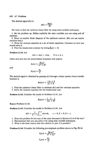
627. Finite-time, Nonstationary Processes (Kalman-Bucy Filters) 611
w(u)
a(u)
>---•r(u), OSu;S;t
Fig. P6.14
and the processes are uncorrelated.
d(t) = a(t).
1. Find the optimum realizable linear filter by using a state-variable formulation.
2. Solve the variance equation for t--+- oo. (You may assume that a statistical
steady state exists.) Observe that a(u), not y1(t), is the message of interest.
Problem 6.3.45. Estimation in Colored Noise. In this problem we consider a simple
example of state-variable estimation in colored noise. Our approach is simpler than
that in the text because we are required to estimate only one state variable. Consider
the following system.
.h(t) = -k1 x1(t) + u1(t),
x2(t) = -k2 x2(t) + u2(t).
We observe
E[u1(t) u2(T)] = 0,
E[u1(t) u1(T)] =2k1P1 8(t- T),
E[u2(t) u2(T)] = 2k1P2 ll(t- T),
E[x12(0)] = P1,
E[x22(0)] = P2,
E[x1(0) x2(0)) = 0.
r(t) = x1(t) + x2(t);
that is, no white noise is present in the observation. We want to apply whitening
concepts to estimating x1(t) and x2(t). First we generate a signal r'(t) which has a
white component.
1. Define a linear transformation of the state variables by
Note that one of our new state variables, Y2(t), is tr(t); therefore, it is known at the
receiver.
Find the state equations for y(t).
2. Show that the new state equations may be written as
where
:YI(t) = -k'y1(t) + [u'(t) + m,(t)]
r'(t) = ;Mt) + k'y2(t) = C'y1(t) + w'(t),
k' = (kl + k2),
2
, - -(kl- k2)
c - 2 ,
u'(t) = tlu1(t) - u2(t)],
w'(t) = t[u1(t) + u2(t)],
m,(t) = C'y2(t).

628. 612 6.7 Problems
Notice that m,(t) is a known function at the receiver; therefore, its effect upon y1(t)
is known. Also notice that our new observation signal r'(t) consists of a linear modu-
lation of Y1(t) plus a white noise component.
3. Apply the estimation with correlated noise results to derive the Kalman-Bucy
realizable filter equations.
4. Find equations which relate the error variance of .X1(t) to
E[(j(t) - Yl(t))2 ] Q P.(t).
5. Specialize your results to the case in which k1 = k2 • What does the variance
equation become in the limit as t-+ oo? Is this intuitively satisfying?
6. Comment on how this technique generalizes for higher dimension systems when
there is no white noise component present in the observation. In the case of multiple
observations can we ever have a singular problem: i.e., perfect estimation?
Comment. The solution to the unrealizable filter problem was done in a different
manner in [56].
Problem 6.3.46. Let
where
d(T) = -km0 0(T) + U(T),
r(T) = a(-r) + w(-r),
E[a(O)] = 0, E[a2(0)] = u2 /2km0 ,
0 =:;:; 'T =:;:; t,
0 5 T 5 f,
Assume that we are processing r(-r) by using a realizable filter which is optimum for
the above message model. The actual message process is
0 =:;:; 'T =:;:; t.
Find the equations which specify tac(t), the actual error variance.
P6.4 Linear Modulation, Communications Context
Problem 6.4.1. Write the variance equation for the DSB-AM example discussed on
p. 576. Draw a block diagram of the system to generate it and verify that the high-
frequency terms can be ignored.
Problem 6.4.2. Let
s(t, a(t)) = v'p [a(t) cos (wet + 8) - ti(t) sin (wet + 8)],
where
A(jw) = H(jw) A(jw).
H(jw) is specified by (506) and 8 is independent of a(t) and uniformly distributed
(0, 277). Find the power-density spectrum of s(t, a(t)) in terms of S.(w).
Problem 6.4.3. In this problem we derive the integral equation that specifies the
optimum estimate of a SSB signal [see (505, 506)]. Start the derivation with (5.25)
and obtain (507).

629. Linear Modulation, Communications Context 613
Problem 6.4.4. Consider the model in Problem 6.4.3. Define
[a(t)]
a(t) = •
ii(t)
Use the vector process estimation results of Section 5.4 to derive (507).
Problem 6.4.5.
1. Draw the block diagram corresponding to (508).
2. Use block diagram manipulation and the properties of H(jw) given in (506) to
obtain Fig. 6.62.
Problem 6.4.6. Let
( p )y,
s(t, a(t)) = 1 + m• [1 + ma(t)] cos w0 t,
where
2k
Sa(w) = w• + k2 •
The received waveform is
r(t) = s(t, a(t)) + w(t), -oo < t < oo
where w(t) is white (No/2). Find the optimum unrealizable demodulator and plot the
mean-square error as a function of m.
Problem 6.4.7(continuation). Consider the model in Problem 6.4.6. Let
1
Sa(w) = 2 W'
0,
JwJ S 21TW,
elsewhere.
Find the optimum unrealizable demodulator and plot the mean-square error as a
function of m.
Problem 6.4.8. Consider the example on p. 583. Assume that
and
2k
Sa(w) = w2 + k2•
1. Find an expression for the mean-square error using an unrealizable demodu-
lator designed to be optimum for the known-phase case.
2. Approximate the integral in part 1 for the case in which Am » 1.
Problem 6.4.9 (continuation). Consider the model in Problem 6.4.8. Let
Repeat Problem 6.4.8.
1
Sa(w) = 2W'
0,
JwJ S 21TW,
elsewhere.

630. 614 6.7 Problems
r(t) Bandpass Square Low-pass
a(t)
filter law filter
We:!: 27rW device hL(T)
Fig. P6.15
Problem 6.4.10. Consider the model in Problem 6.4.7. The demodulator is shown in
Fig. P6.15. Assume m « 1 and
1
Sa(w) = 2 W'
0, elsewhere,
where 21r( W1 + W) « we.
Choose hL(,.) to minimize the mean-square error. Calculate the resulting error ~P·
P6.6 Related Issues
In Problems 6.6.1 through 6.6.4, we show how the state-variable techniques we have
developed can be used in several important applications. The first problem develops
a necessary preliminary result. The second and third problems develop a solution
technique for homogeneous and nonhomogeneous Fredholm equations (either vector
or scalar). The fourth problem develops the optimum unrealizable filter. A complete
development is given in [54]. The model for the four problems is
x(t) = F(t)x(t) + G(t)u(t)
y(t) = C(t)x(t)
E[u(t)uT('T)] = Qll(t - T)
We use a function ;(t) to agree with the notation of [54]. It is not related to the
variance matrix !f;p(t).
Problem 6.6.1. Define the linear functional
where s(t) is a bounded vector function.
We want to show that when Kx(t, T) is the covariance matrix for a state-variable
random process x(t) we can represent this functional as the solution to the differential
equations
and
d~~) = F(t) If;(I) + G(t) QGT(t) lJ(I)
d~~) = -FT(t) l](t) - s(t),
with the boundary conditions
lJ(T1) = 0,
and
;(T1) = P0lJ(T,),
where
Po = Kx(T" ]j).

631. Related Issues 615
1. Show that we can write the above integral as
il l~
;{t) = 4»(t, r) Kx(T, r) s(r) dr + Kx(t, t)4»T(r, t) s(r) dr.
~ I
Hint. See Problem 6.3.16.
2. By using Leibnitz's rule, show that
Hint. Note that Kx(t, t) satisfies the differential equation
dKd~' t) = F(t) Kx(t, t) + Kx(t, t)FT(t) + G(t)QGT(t), (text 273)
with Kx(T~o T1) = P0 , and 4»T(,-, t) satisfies the adjoint equation; that is,
with 4»(T., T,) = I.
3. Define a second functionall](t) by
Show that it satisfies the differential equation
4. Show that the differential equations must satisfy the two independent boundary
conditions
lJ(T1) = 0,
;(T1) = P0lJ(T,).
5. By combining the results in parts 2, 3, and 4, show the desired result.
Problem 6.6.2. Homogeneous Fredholm Equation. In this problem we derive a set of
differential equations to determine the eigenfunctions for the homogeneous Fredholm
equation. The equation is given by
iT!
Ky(t, r)<j>(r) dr = .<j>(t),
T,
or
for,> 0.
Define
so that
I 1
<j>(t) = XC(t) ;(t).

632. 616 6.7 Problems
1. Show that l;(t) satisfies the differential equations
d f"l;U>]
di Ll)ct) =
with
I;(T,) = P0YJ(T,),
7J(T1) = 0.
(Use the results of Problem 6.6.1.)
2. Show that to have a nontrivial solution which satisfies the boundary conditions
we need
det ['I'.~(T,, T,: >.)Po + 'I'••(T" T,: .>.)] = 0,
where 'l'(t, T,: .>.) is given by
d ['l'~~(t, T,: .>.) : 'l'~.(t, T,: .>.)]
dt '¥.~(~-:;.~>.)- i-'i.~(t~-:r.~>.)
[
____!~!}_____ :_~~~_<?~~(~~] [~:~~~_:•_:_.>.~- -!~~~~~ -~·~~~]
= -CT(t) C(t) : T . . '
.>. : -F (t) 'l'.,(t, T, . .>.) '1'nnCt. T, . .>.)
and 'I'(T;, T,: .>.) = I. The values of.>. which satisfy this equation are the eigenvalues.
3. Show that the eigenfunctions are given by
where l)(T,) satisfies the orthogonality relationship
['I'.~(T,, T,:.>.) Po + 'I'••(T,, 71: .>.)] YJ(T,) = 0.
Problem 6.6.3. Nonhomogeneous Fredholm Equation. In this problem we derive a set
of differential equations to determine the solution to the nonhomogeneous Fredholm
equation. This equation is given by
IT!
Ky(t, -r)g(-r)d-r + ag(t) = s(t),
Tt
I. If we define l;(t) as
T, :::;; t :::;; T1, a > 0.
show that we may write the nonhomogeneous equation as
1
g(t) =- [s(t) - C(t) l;(t)].
a
2. Using Problem 6.6.1, show that ;ct) satisfies the differential equations

633. with
~(Tt) = Po l)(Tt),
'l)(T1) = 0.
Related Issues 617
Comment. In general we can replace a by an arbitrary positive-definite time-varying
matrix (R(t)) and the derivation is valid with obvious modifications.
Problem No. 6.6.4. Unrealizable Filters. In this problem we show how the nonhomo-
geneous Fredholm equation may be used to determine the optimal unrealizable
filter structure. For algebraic simplicity we assume r(t) is a scalar.
R(t) = N0/2.
1. Show that the integral equation specifying the optimum unrealizable filter for
estimating x(l) at any point tin the interval [Ti, T1] is
Ti < T < T,. (1)
2. Using the inverse kernel of K,(t, T) [Chapter 4, (4.161)] show that
i(l) = I:.'Kx(t, T)CT(T)(f:.' Q,(T, o) r(o) do), (2)
3. As in Chapter 5, define the term in parentheses as r0(T). We note that r.tT) solves
the nonhomogeneous Fredholm equation when the input is r(l). Using Problem No.
6.6.3, show that r0(1) is given by
2
r9(t) = No (r(l) - C(l~(t)), (3)
where
d~~l) = F(t)~(t) + G(t)QGT(t)'l),(t), (4a)
and
J;(T,) = Kx(Ti, Tt)l),(T,),
'l) 1(T1) = 0.
(Sa)
(5b)
4. Using the results of Problem No. 6.6.1, show that i(t) satisfies the differential
equation,
where
d~;t) = F(l)i(l) + G(t)QGT(t)'l)2(t),
d~~t) = - CT(t)r0(1) - FT(I)'l)2(1),
i(Tt) = Kx(Tt. Ti)'l)2(T,),
'l•(T1) = 0.
5. Substitute (3) into (6b). Show that
and
7),(1) = '12(1),
i(l) = ~(1).
(6a)
(6b)
(7a)
(1b)
(Sa)
(Sb)

634. 618 6.7 Problems
6. Show that the differential equation structure for the optimum unrealizable
estimate of i(t) is
where
Comments
d"(t)
~t = F(t)x(t) + G(t)QGT(t)'t)(t),
d~~t) = CT(t) ~o C(t)x(t) - FT(t)'t)(t) - CT(t) ~o r(t),
i(1j) = Kx(Tt. 1i)TJ(1i),
't)(Tr) = 0.
1. We have two n-dimensionallinear vector differential equations to solve.
(9a)
(9b)
(lOa)
(lOb)
2. The performance given by the unrealizable error covariance matrix is not part
of the filter structure.
3. By letting Tr be a variable we can determine a differential equation structure
for i(Tr) as a function of T1. These equations are just the Kalman-Bucy equations for
the optimum realizable filter.
Problem 6.6.5. In Problems 6.2.29 and 6.2.30 we discussed a realizable whitening
filter for infinite intervals and stationary processes. In this problem we verify that
these results generalize to finite intervals and nonstationary processes.
Let
r('r) = nc(-r) + w(-r),
where nc(-r) can be generated as the output of a dynamic system,
driven by white noise u(t).
Show that the process
is white.
i(t) = F(t)x(t) + G(t)u(t)
nc(t) = C(t)x(t),
r'(t) = r(t) - fie(!),
= r(t) - C(t)x(t),
Problem 6.6.6. Sequential Estimation. Consider the convolutional encoder in Fig. P6.16.
I. What is the "state" of this system?
2. Show that an appropriate set of state equations is
[ ::::: :] = [~ 0 ~] [::::] EB [~] u.
Xa,n +1 0 0 0 Xa,n 1
Xn+l =
Yn+l = [I O
1 1
(all additions are modulo 2).
~] [::::::]
Xa,n+ 1
Assume that the process u is composed of a sequence of independent binary random
variables with
E(u. = 0) = P.,
E(un = 1) = 1 - P•.

635. References 619
(Sequence of binary digits
~ %3 %2
0101 Shift register
~----+---------~Yl
....________________,._ Y2 ·
Fig. P6.16
In addition, assume that the components of y are sent over two independent identical
binary symmetric channels such that
where
rn = Y E8 w,
E(wn,l = 0) = Pw,
E(wn,l = 1) = 1 - Pw•
Finally, let the sequence of measurements
rh r2, ... , rn, be denoted by Zn.
3. Show that the a posteriori probability density Pxn+1lzn+1(Xn+dZn+l) satisfies
the following recursive relationship:
Pxn+ 1lzn+ l(Xn+ dZn+l)
Prn+ 1Jzn+ l(Rn+liXn+l) LPxn+ lJxn(Xn+dXn)Pxnlzn(XniZn)
Xn
L Prn+1Jxn+l(Rn+ dXn+ 1) LPxn+ lJxn(Xn+dXn)Pxnlzn(XniZn)
Xn+l Xn
where Lx. denotes the sum over all possible states.
4. How would you design the MAP receiver that estimates Xn+l? What must be
computed for each receiver estimate?
5. How does this estimation procedure compare with the discrete Kalman filter?
6. How does the complexity of this procedure increase as the length of the con-
volutio-nal encoder increases?
REFERENCES
[1] N. Wiener, The Extrapolation, Interpolation, and Smoothing of Stationary Time
Series, Wiley, New York, 1949.
[2] A. Kolmogoroff, "Interpolation and Extrapolation," Bull. Acad. Sci., U.S.S.R.,
Ser. Math., S, 3-14 (1941).
[3] H. W. Bode and C. E. Shannon, "A Simplified Derivation of Linear Least-
squares Smoothing and Prediction Theory," Proc. IRE, 38, 417-426 (1950).
[4] M. C. Yovits and J. L. Jackson," Linear Filter Optimization with Game Theory
Considerations," IRE·Nationa/ Convention Record, Pt. 4, 193-199 (1955).
[5] A. J. Viterbi and C. R. Cahn, "Optimum Coherent Phase and Frequency

636. 620 References
Demodulation of a Class of Modulating Spectra," IEEE Trans. Space Electronics
and Telemetry, SET-10, No. 3, 95-102 (September 1964).
[6] D. L. Snyder, "Some Useful Expressions for Optimum Linear Filtering in
White Noise," Proc. IEEE, 53, No. 6, 629-630 (1965).
[7] C. W. Helstrom, Statistical Theory of Signal Detection, Pergamon, New York,
1960.
[8] W. C. Lindsay, "Optimum Coherent Amplitude Demodulation," Proc. NEC,
20, 497-503 (1964).
[9] G. C. Newton, L.A. Gould, and J. F. Kaiser, Analytical Design ofLinear Feed-
back Controls, Wiley, New York, 1957.
[10] E. Wong and J. B. Thomas, "On the Multidimensional Filtering and Prediction
Problem and the Factorization of Spectral Matrices," J. Franklin Inst., 8, 87-99,
(1961).
[11] D. C. Youla, "On the Factorization of Rational Matrices," IRE Trans. Inform.
Theory, IT-7, 172-189 (July 1961).
[12] R. C. Amara, "The Linear Least Squares Synthesis of Continuous and Sampled
Data Multivariable Systems," Report No. 40, Stanford Research Laboratories,
1958.
[13] R. Brockett, ''Spectral Factorization of Rational Matrices," IEEE Trans.
Inform. Theory (to be published).
[14] M. C. Davis, "On Factoring the Spectral Matrix," Joint Automatic Control
Conference, Preprints, pp. 549-466, June 1963; also, IEEE Transactions on
Automatic Control, 296-305, October 1963.
[15] R. J. Kavanaugh, "A Note on Optimum Linear Multivariable Filters," Proc.
Inst. Elec. Engs., 108, Pt. C, 412-217, Paper No. 439M, 1961.
[16] N. Wiener and P. Massani, "The Prediction Theory of Multivariable Stochastic
Processes," Acta Math., 98 (June 1958).
[17] H. C. Hsieh and C. T. Leondes, "On the Optimum Synthesis of Multipole
Control Systems in the Wiener Sense," IRE Trans. on Automatic Control,
AC-4, 16-29 (1959).
[18] L. G. McCracken, "An Extension of Wiener Theory of Multi-Variable Controls,"
IRE International Convention Record, Pt. 4, p. 56, 1961.
[19] H. C. Lee, "Canonical Factorization of Nonnegative Hermetian Matrices,"
J. London Math. Soc., 23, 100-110 (1948).
[20] M. Mohajeri, "Closed-form Error Expressions," M.Sc. Thesis, Dept. of
Electrical Engineering, M.I.T., 1968.
[21] D. L. Snyder, "The State-Variable Approach to Continuous Estimation," M.I.T.,
Sc.D. Thesis, February 1966.
[22] C. L. Dolph and M.A. Woodbury," On the Relation Between Green's Functions
and Covariances of Certain Stochastic Processes and its Application to Unbiased
Linear Prediction," Trans. Am. Math. Soc., 1948.
[23] R. E. Kalman and R. S. Bucy, "New Results in Linear Filtering and Prediction
Theory," ASME J. Basic Engr., March 1961.
[24] L.A. Zadeh and C. A. DeSoer, Linear System Theory, McGraw-Hill, New York,
1963.
[25] S. C. Gupta, Transform and State Variable Methods in Linear Systems, Wiley,
New York, 1966.
[26] M. Athans and P. L. Falb, Optimal Control, McGraw-Hill, New York, 1966.
[27] P. M. DeRusso, R. J. Roy, and C. M. Close, State Variables for Engineers,
Wiley, New York, 1965.

637. References 621
[28] R. J. Schwartz and B. Friedland, Linear Systems, McGraw-Hill, New York,
1965.
[29] E. A. Coddington and N. Levinson, Theory of Ordinary Differential Equations,
McGraw-Hill, New York, 1955.
[30] R. E. Bellman, Stability Theory of Differential Equations, McGraw-Hill, New
York, 1953.
[31] N. W. McLachlan, Ordinary Non-linear Differential Equations in Engineering
and Physical Sciences, Clarendon Press, Oxford, 1950.
[32] J. J. Levin, "On the Matrix Riccati Equation," Proc. Am. Math. Soc., 10,
519-524 (1959).
[33] W. T. Reid, "Solutions of a Riccati Matrix Differential Equation as Functions
of Initial Values," J. Math. Mech., 8, No. 2 (1959).
[34] W. T. Reid, "A Matrix Differential Equation of Riccati Type," Am. J. Math.,
68, 237-246 (1946); Addendum, ibid., 70, 460 (1948).
[35] W. J. Coles, "Matrix Riccati Differential Equations," J. Soc. Indust. Appl.
Math., 13, No. 3 (September 1965).
[36] A. B. Baggeroer, "Solution to the Ricatti Equation for Butterworth Processes,"
Internal Memo., Detection and Estimation Theory Group, M.I.T., 1966.
[37] E. A. Guillemin, Synthesis ofPassive Networks, Wiley, New York, 1957.
[38] L. Weinberg, Network Analysis and Synthesis, McGraw-Hill, New York.
[39] D. L. Snyder, "Optimum Linear Filtering of an Integrated Signal in White
Noise," IEEE Trans. Aerospace Electron. Systems, AES-2, No. 2, 231-232
(March 1966).
[40] A. B. Baggeroer, "Maximum A Posteriori Interval Estimation," WESCON,
Paper No. 7/3, August 23-26, 1966.
[41] A. E. Bryson and D. E. Johansen, "Linear Filtering for Time-Varying Systems
Using Measurements Containing Colored Noise," IEEE Transactions on Auto-
matic Control, AC-10, No. 1 (January 1965).
[42] L. D. Collins, "Optimum Linear Filters for Correlated Messages and Noises,"
Internal Memo. 17, Detection and Estimation Theory Group, M.I.T., October
28, 1966.
[43] A. B. Baggeroer and L. D. Collins, "Maximum A Posteriori Estimation in
Correlated Noise," Internal Memo., Detection and Estimation Theory Group,
M.I.T., October 25, 1966.
[44] H. L. Van Trees, "Sensitivity Equations for Optimum Linear Filters," Internal
Memorandum, Detection and Estimation Theory Group, M.I.T., February
1966.
[45] J. B. Thomas, "On the Statistical Design of Demodulation Systems for Signals
in Additive Noise," TR-88, Stanford University, August 1955.
[46] R. C. Booton, Jr., and M. H. Goldstein, Jr., "The Design and Optimization of
Synchronous Demodulators," IRE Wescon Convention Record, Part 2, 154-170,
1957.
[47] "Single Sideband Issue," Proc. IRE, 44, No. 12, (December 1956).
[48] J. M. Wozencraft, Lectures on Communication System Theory, E. J. Baghdady,
ed., McGraw-Hill, New York, Chapter 12, 1961.
[49] M. Schwartz, Information Transmission, Modulation, and Noise, McGraw-Hill
Co., New York, 1959.
[50] J. P. Costas, "Synchronous Communication," Proc. IRE, 44, 1713-1718
(December 1956).
[5l]R. Jaffe and E. Rechtin, "Design and Performance of Phase-Lock Circuits

638. 622 References
Capable of Near-optimum Performance over a Wide Range of Input Signal and
Noise Levels," IRE Trans. Inform. Theory, IT-1, 66-76 (March 1955).
[52] A. B. Baggeroer, "A State Variable Technique for the Solution of Fredholm
Integral Equations," Proc. 1967 Inti. Conf. Communications, Minneapolis,
Minn., June 12-14, 1967.
[53] A. B. Baggeroer and L. D. Collins, "Evaluation of Minimum Mean Square
Error for Estimating Messages Whose Spectra Belong to the Gaussian Family,"
Internal Memo, Detection and Estimation Theory Group, M.I.T., R.L.E., July
12, 1967.
[54] A. B. Baggeroer, "A State-Variable Approach to the Solution of Fredholm
Integral Equations," M.I.T., R.L.E. Technical Report 459, July 15, 1967.
[55] A. Papoulis, Probability, Random Variables, and Stochastic Processes, McGraw-
Hill Co., New York, 1965.
[56] A. E. Bryson and M. Frazier, "Smoothing for Linear and Nonlinear Dynamic
Systems," USAF Tech. Rpt. ASD-TDR-63-119 (February 1963).

639. 7
Discussion
Detection, Estimation, and Modulation Theory, Part I:
Detection, Estimation, and Linear Modulation Theory. Harry L. Van Trees
Copyright © 2001 John Wiley & Sons, Inc.
ISBNs: 0-471-09517-6 (Paperback); 0-471-22108-2 (Electronic)
The next step in our development is to apply the results in Chapter 5 to
the nonlinear estimation problem. In Chapter 4 we studied the problem of
estimating a single parameter which was contained in the observed signal
in a nonlinear manner. The discrete frequency modulation example we
discussed illustrated the type of difficulties met. We anticipate that even
more problems will appear when we try to estimate a sample function
from a random process. This conjecture turns out to be true and it forces
us to make several approximations in order to arrive at a satisfactory
answer. To make useful approximations it is necessary to consider specific
nonlinear estimation problems rather than the general case. In view ofthis
specialization it seems appropriate to pause and summarize what we have
already accomplished. In Chapter 2 of Part II we shall discuss nonlinear
estimation. The remainder of Part II discusses random channels, radar/
sonar signal processing, and array processing. In this brief chapter we
discuss three issues.
1. The problem areas that we have studied. These correspond to the
first two levels in the hierarchy outlined in Chapter 1.
2. The problem areas that remain to be covered when our development
is resumed in Part II.
3. Some areas that we have encountered in our discussion that we do
not pursue in Part II.
7.1 SUMMARY
Our initial efforts in this book were divided into developing background
in the area ofclassical detection and estimation theory and random process
representation. Chapter 2 developed the ideas of binary and M-ary
623

640. 624 7.1 Summary
hypothesis testing for Bayes and Neyman-Pearson criteria. The funda-
mental role of the likelihood ratio was developed. Turning to estimation
theory, we studied Bayes estimation for random parameters and maximum-
likelihood estimation for nonrandom parameters. The idea of likelihood
functions, efficient estimates, and the Cramer-Rao inequality were of
central importance in this discussion. The close relation between detection
and estimation theory was emphasized in the composite hypothesis testing
problem. A particularly important section from the standpoint of the
remainder of the text was the general Gaussian problem. The model was
simply the finite-dimensional version of the signals in noise. problems
which were the subject of most of our subsequent work. A section on
performance bounds which we shall need in Chapter 11.3 concluded the
discussion of the classical problem.
In Chapter 3 we reviewed some of the techniques for representing
random processes which we needed to extend the classical results to the
waveform problem. Emphasis was placed on the Karhunen-Loeve expan-
sion as a method for obtaining a set of uncorrelated random variables as
a representation ofthe process over a finite interval. Other representations,
such as the Fourier series expansion for periodic processes, the sampling
theorem for bandlimited processes, and the integrated transform for
stationary processes on an infinite interval, were also developed. As pre-
paration for some of the problems that were encountered later in the text,
we discussed various techniques for solving the integral equation that
specified the eigenfunctions and eigenvalues. Simple characterizations for
vector processes were also obtained. Later, in Chapter 6, we returned to
the representation problem and found that the state-variable approach
provided another method of representing processes in terms of a set of
random variables. The relation between these two approaches is further
developed in [I] (see Problem 6.6.2 of Chapter 6).
The next step was to apply these techniques to the solution of some basic
problems in the communications and radar areas. In Chapter 4 we studied
a large group of basic problems. The simplest problem was that of detect-
ing one of two known signals in the presence of additive white Gaussian
noise. The matched filter receiver was the first important result. The ideas
of linear estimation and nonlinear estimation of parameters were derived.
As pointed out at that time, these problems corresponded to engineering
systems commonly referred to as uncoded PCM, PAM, and PFM,
respectively. The extension to nonwhite Gaussian noise followed easily. In
this case it was necessary to solve an integral equation to find the functions
used in the optimum receiver, so we developed techniques to obtain these
solutions. The method for dealing with unwanted parameters such as a
random amplitude or random phase angle was derived and some typical

641. Preview ofPart II 625
cases were examined in detail. Finally, the extensions to multiple-parameter
estimation and multiple-channel systems were accomplished. At this point
in our development we could design and analyze digital communication
systems and time-sampled analog communication systems operating in a
reasonably general environment.
The third major area was the estimation of continuous waveforms. In
Chapter 5 we approached the problem from the viewpoint of maximum a
posteriori probability estimation. The primary result was a pair of integral
equations that the optimum estimate had to satisfy. To obtain solutions
we divided the problem into linear estimation which we studied in Chapter
6 and nonlinear estimation which we shall study in Chapter 11.2.
Although MAP interval estimation served as a motivation and intro-
duction to Chapter 6, the actual emphasis in the chapter was on minimum
mean-square point estimators. After a briefdiscussion ofgeneral properties
we concentrated on two classes of problems. The first was the optimum
realizable point estimator for the case in which the processes were station-
ary and the infinite past was available. Using the Wiener-Hopf spectrum
factorization techniques, we derived an algorithm for obtaining the
form expressions for the errors. The second class was the optimum
realizable point estimation problem for finite observation times and
possibly nonstationary processes. After characterizing the processes by
using state-variable methods, a differential equation that implicitly speci-
fied the optimum estimator was derived. This result, due to Kalman and
Bucy, provided a computationally feasible way of finding optimum pro-
cessors for complex systems. Finally, the results were applied to the types
of linear modulation scheme encountered in practice, such as DSB-AM
and SSB.
It is important to re-emphasize two points. The linear processors
resulted from our initial Gaussian assumption and were the best processors
of any kind. The use of the minimum mean-square error criterion was not
a restriction because we showed in Chapter 2 that when the a posteriori
density is Gaussian the conditional mean is the optimum estimate for any
convex (upward) error criterion. Thus the results of Chapter 6 are of far
greater generality than might appear at first glance.
7.2 PREVIEW OF PART II
In Part II we deal with four major areas. The first is the solution of the
nonlinear estimation problem that was formulated in Chapter 5. In
Chapter 11.2 we study angle modulation in detail. The first step is to show
how the integral equation that specifies the optimum MAP estimate
suggests a demodulator configuration, commonly referred to as a phase-
lock loop (PLL). We then demonstrate that under certain signal and noise

642. 626 7.2 Preview ofPart II
conditions the output of the phase-lock loop is an asymptotically efficient
estimate of the message. For the simple case which arises when the PLL
is used for carrier synchronization an exact analysis of the performance
in the nonlinear region is derived. Turning to frequency modulation, we
investigate the design of optimum demodulators in the presence of band-
width and power constraints. We then compare the performance of these
optimum demodulators with conventional limiter-discriminators. After
designing the optimum receiver the next step is to return to the transmitter
and modify it to improve the overall system performance. This modifica-
tion, analogous to the pre-emphasis problem in conventional frequency
modulation, leads to an optimum angle modulation system. Our results in
this chapter and Chapter I.4. give us the background to answer the fol-
lowing question: If we have an analog message to transmit, should we (a)
sample and quantize it and use a digital transmission system, {b) sample it
and use a continuous amplitude-time discrete system,or(c)use a continuous
analog system? In order to answer this question we first use the rate-
distortion results of Shannon to derive bounds on how well any system
could do. We then compare the various techniques discussed above with
these bounds. As a final topic in this chapter we show how state-variable
techniques can be used to derive optimum nonlinear demodulators.
In Chapter 11.3 we return to a more general problem. We first consider
the problem of observing a received waveform r(t) and deciding to which
oftwo random processes it belongs. This type of problem occurs naturally
in radio astronomy, scatter communication, and passive sonar. The likeli-
hood ratio test leads to a quadratic receiver which can be realized in
several mathematically equivalent ways. One receiver implementation, the
estimator-correlator realization, contains the optimum linear filter as a
component and lends further importance to the results in Chapter 1.6.
In a parallel manner we consider the problem of estimating parameters
contained in the covariance function of a random process. Specific prob-
lems encountered in practice, such as the estimation ofthe center frequency
of a bandpass process or the spectral width of a process, are discussed in
detail. In both the detection and estimation cases particularly simple
solutions are obtained when the processes are stationary and the observa-
tion times are long. To complete the hierarchy of problems outlined in
Chapter 1 we study the problem of transmitting an analog message over a
randomly time-varying channel. As a specific example, we study an angle
modulation system operating over a Rayleigh channel.
In Chapter 11.4 we show how our earlier results can be applied to solve
detection and parameter estimation problems in the radar-sonar area.
Because we are interested in narrow-band signals, we develop a representa-
tion for them by using complex envelopes. Three classes of target models

643. Unexplored Issues 627
are considered. The simplest is a slowly fluctuating point target whose
range and.velocity are to be estimated. We find that the issues of accuracy,
ambiguity, and resolution must all be considered when designing signals
and processors. The radar ambiguity function originated by Woodward
plays a central role in our discussion. The targets in the next class are
referred to as singly spread. This class includes fast-fluctuating point
targets which spread the transmitted signal in frequency and slowly
fluctuating dispersive targets which spread the signal in time (range). The
third class consists of doubly spread targets which spread the signal in
both time and frequency. Many diverse physical situations, such as
reverberation in active sonar systems, communication over scatter chan-
nels, and resolution in mapping radars, are included as examples. The over-
all development provides a unified picture of modern radar-sonar theory.
The fourth major area in Part II is the study of multiple-process and
multivariable process problems. The primary topic in this area is a detailed
study of array processing in passive sonar (or seismic) systems. Optimum
processors for typical noise fields are analyzed from the standpoint of
signal waveform estimation accuracy, detection performance, and beam
patterns. Two other topics, multiplex transmission systems and multi·
variable systems (e.g., continuous receiving apertures or optical systems),
are discussed briefly.
In spite of the length of the two volumes, a number of interesting topics
have been omitted. Some of them are outlined in the next section.
7.3 UNEXPLORED ISSUES
Several times in our development we have encountered interesting ideas
whose complete discussion would have taken us too far afield. In this
section we provide suitable references for further study.
Coded Digital Communication Systems. The most important topic we
have not discussed is the use of coding techniques to reduce errors in
systems that transmit sequences of digits. Shannon's classical information
theory results indicate how well we can do, and a great deal of research
has been devoted to finding ways to approach these bounds. Suitable texts
in this area are Wozencraft and Jacobs [2], Fano [3], Gallager [4],
Peterson [5], and Golomb [6]. Bibliographies of current papers appear in
the "Progress in Information Theory" series [7] and [8].
Sequential Detection and Estimation Schemes. All our work has dealt
with a fixed observation interval. Improved performance can frequently be
obtained if a variable length test is allowed. The fundamental work in this
area is due to Wald [10]. It was applied to the waveform problem by

644. 628 7.3 Unexplored Issues
Peterson, Birdsall, and Fox [11] and Bussgang and Middleton [12]. Since
that time a great many papers have considered various aspects of the
subject (e.g. [13] to [22]).
Nonparametric Techniques. Throughout our discussion we have assumed
that the random variables and processes have known density functions.
The nonparametric statistics approach tries to develop tests that do not
depend on the density function. As we might expect, the problem is more
difficult, and even in the classical case there are a number of unsolved
problems. Two books in the classical area are Fraser [23] and Kendall [24].
Other references are given on pp. 261-264 of [25] and in [26]. The progress
in the waveform case is less satisfactory. (A number of models start by
sampling the input and then use a known classical result.) Some recent
interesting papers include [27] to [32].
Adaptive and Learning Systems. Ever-popular adjectives are the words
"adaptive" and "learning." By a suitable definition of adaptivity many
familiar systems can be described as adaptive or learning systems. The
basic notion is straightforward. We want to build a system to operate
efficiently in an unknown or changing environment. By allowing the system
to change its parameters or structure as a function of its input, the per-
formance can be improved over that of a fixed system. The complexity of
the system depends on the assumed model of the environment and the
degrees offreedom that are allowed in the system. There are a large number
of references in this general area. A representative group is [33] to [50]
and [9].
Pattern Recognition. The problem of interest in this area is to recognize
(or classify) patterns based on some type of imperfect observation. Typical
areas of interest include printed character recognition, target classifica-
tion in sonar systems, speech recognition, and various medical areas such
as cardiology. The problem can be formulated in either a statistical or
non-statistical manner. Our work would be appropriate to a statistical
formulation.
In the statistical formulation the observation is usually reduced to an
N-dimensional vector. Ifthere are M possible patterns, the problem reduces
to the finite dimensional M-hypothesis testing problem of Chapter 2. If we
further assume a Gaussian distribution for the measurements, the general
Gaussian problem of Section 2.6 is directly applicable. Some typical
pattern recognition applications were developed in the problems ofChapter
2. A more challenging problem arises when the Gaussian assumption is
not valid; [8] discusses some of the results that have been obtained and
also provides further references.

645. References 629
Discrete Time Processes. Most of our discussion has dealt with observa-
tions that were sample functions from continuous time processes. Many of
the results can be reformulated easily in terms of discrete time processes.
Some of these transitions were developed in the problems.
Non-Gaussian Noise. Starting with Chapter 4, we confined our work to
Gaussian processes. As we pointed out at the end of Chapter 4, various
types of result can be obtained for other forms of interference. Some
typical results are contained [51] to [57].
Receiver-to-Transmitter Feedback Systems. In many physical situations
it is reasonable to have a feedback link from the receiver to the transmitter.
The addition of the link provides a new dimension in system design and
frequently enables us to achieve efficient performance with far less com-
plexity than would be possible in the absence of feedback. Green [58]
describes the work in the area up to 1961. Recent work in the area includes
[59] to [63] and [76].
Physical Realizations. The end product of most of our developments
has been a block diagram of the optimum receiver. Various references
discuss practical realizations of these block diagrams. Representative
systems that use the techniques of modem communication theory are
described in [64] to [68].
Markov Process-Differential Equation Approach. With the exception of
Section 6.3, our approach to the detection and estimation problem could
be described as a "covariance function-impulse response" type whose
success was based on the fact that the processes ofconcern were Gaussian.
An alternate approach could be based on the Markovian nature of the
processes of concern. This technique might be labeled the "state-variable-
differential equation" approach and appears to offer advantages in many
problems: [69] to [75] discuss this approach for some specific problems.
Undoubtedly there are other related topics that we have not mentioned,
but the foregoing items illustrate the major ones.
REFERENCES
[1] A. B. Baggeroer, "Some Applications of State Variable Techniques in Com-
munications Theory," Sc.D. Thesis, Dept. of Electrical Engineering, M.I.T.,
February 1968.
[2] J. M. Wozencraft and I. M. Jacobs, Principles of Communication Engineering,
Wiley, New York, 1965.
[3] R. M. Fano, The Transmission of Information, The M.I.T. Press and Wiley,
New York, 1961.

646. 630 References
[4] R. G. Gallager, Notes on Information Theory, Course 6.574, M.I.T.
[5] W. W. Peterson, Error-Correcting Codes, Wiley, New York, 1961.
[6] S. W. Golomb (ed.), Digital Communications with Space Applications, Prentice-
Hall, Englewood Cliffs, New Jersey, 1964.
[7] P. Elias, A. Gill, R. Price, P. Swerling, L. Zadeh, and N. Abramson; "Progress
in Information Theory in the U.S.A., 1957-1960," IRE Trans. Inform. Theory,
IT-7, No. 3, 128-143 (July 1960).
[8] L. A. Zadeh, N. Abramson, A. V. Balakrishnan, D. Braverman, M. Eden,
E. A. Feigenbaum, T. Kailath, R. M. Lerner, J. Massey, G. E. Mueller, W. W.
Peterson, R. Price, G. Sebestyen, D. Slepian, A. J. Thomasian, G. L. Turin,
"Report on Progress in Information Theory in the U.S.A., 196o-1963," IEEE
Trans. Inform. Theory, IT-9, 221-264 (October 1963).
[9] M. E. Austin, "Decision-Feedback Equalization for Digital Communication
Over Dispersive Channels," M.I.T. Sc.D. Thesis, May 1967.
[10] A. Wald, Sequential Analysis, Wiley, New York, 1947.
[11] W. W. Peterson, T. G. Birdsall, and W. C. Fox, "The Theory of Signal Detect-
ability," IRE Trans. Inform. Theory, PGIT-4, 171 (1954).
[12] J. Bussgang and D. Middleton, "Optimum Sequential Detection of Signals in
Noise," IRE Trans. Inform. Theory, IT-1, 5 (December 1955).
[13] H. Blasbalg, "The Relationship of Sequential Filter Theory to Information
Theory and Its Application to the Detection of Signals in Noise by Bernoulli
Trials," IRE Trans. Inform. Theory, IT-3, 122 (June 1957); Theory of Sequential
Filtering and Its Application to Signal Detection and Classification, doctoral
dissertation, Johns Hopkins University, 1955; "The Sequential Detection of a
Sine-wave Carrier of Arbitrary Duty Ratio in Gaussian Noise," IRE Trans.
Inform. Theory, IT-3, 248 (December 1957).
[14] M. B. Marcus and P. Swerling, "Sequential Detection in Radar With Multiple
Resolution Elements," IRE Trans. Inform. Theory, IT-8, 237-245 (April 1962).
[15] G. L. Turin, "Signal Design for Sequential Detection Systems With Feedback,"
IEEE Trans. Inform. Theory, IT-11, 401-408 (July 1965); "Comparison of
Sequential and Nonsequential Detection Systems with Uncertainty Feedback,"
IEEE Trans. Inform. Theory, IT-12, 5-8 (January 1966).
[16] A. J. Viterbi, "The Effect of Sequential Decision Feedback on Communication
over the Gaussian Channel," Information and Control, 8, So-92 (February 1965).
[17] R. M. Gagliardi and I. S. Reed, "On the Sequential Detection of Emerging
Targets," IEEE Trans. Inform. Theory, IT-11, 26o-262 (April1965).
[18] C. W. Helstrom, "A Range Sampled Sequential Detection System," IRE Trans.
Inform. Theory, IT-8, 43-47 (January 1962).
[19] W. Kendall and I. S. Reed, "A Sequential Test for Radar Detection of Multiple
Targets," IRE Trans. Inform. Theory, IT-9, 51 (January 1963).
[20] M. B. Marcus and J. Bussgang, "Truncated Sequential Hypothesis Tests,"
The RAND Corp., RM-4268-ARPA, Santa Monica, California, November
1964.
[21] I. S. Reed and I. Selin, "A Sequential Test for the Presence of a Signal in One
of k Possible Positions," IRE Trans. Inform. Theory, IT-9, 286 (October 1963).
[22] I. Selin, "The Sequential Estimation and Detection of Signals in Normal Noise,
I," Information and Control, 7, 512-534 (December 1964); "The Sequential
Estimation and Detection of Signals in Normal Noise, II," Information and
Control, 8, 1-35 (January 1965).
[23] D. A. S. Fraser, Nonparametric Methods in Statistics, Wiley, New York, 1957.

647. References 631
[24] M. G. Kendall, Rank Correlation Methods, 2nd ed., Griffin, London, 1955.
[25] E. L. Lehmann, Testing Statistical Hypotheses, Wiley, New York, 1959.
[26] I. R. Savage, "Bibliography of nonparametric statistics and related topics,"
J. American Statistical Association, 48, 844-906 (1953).
[27] M. Kanefsky, "On sign tests and adaptive techniques for nonparametric
detection," Ph.D. dissertation, Princeton University, Princeton, New Jersey,
1964.
[28] S. S. Wolff, J. B. Thomas, and T. Williams, "The Polarity Coincidence Cor-
relator: a Nonparametric Detection Device," IRE Trans. Inform. Theory, IT-8,
1-19 (January 1962).
[29] H. Ekre, "Polarity Coincidence Correlation Detection of a Weak Noise Source,"
IEEE Trans. Inform. Theory, IT-9, 18-23 (January 1963).
[30] M. Kanefsky, "Detection of Weak Signals with Polarity Coincidence Arrays,"
IEEE Trans. Inform. Theory, IT-12 (Apri11966).
[31] R. F. Daly, "Nonparametric Detection Based on Rank Statistics," IEEE Trans.
Inform. Theory, IT-12 (April 1966).
[32] J. B. Millard and L. Kurz, "Nonparametric Signal Detection-An Application
of the Kolmogorov-Smirnov, Cramer-Von Mises Tests," IEEE Trans. Inform.
Theory, IT-12 (April 1966).
[33] C. S. Weaver, "Adaptive Communication Filtering," IEEE Trans. Inform.
Theory, IT-8, S169-Sl78 (September 1962).
[34] A. M. Breipohl and A. H. Koschmann, "A Communication System with
Adaptive Decoding," Third Symposium on Discrete Adaptive Processes, 1964
National Electronics Conference, Chicago, 72-85, October 19-21.
[35] J. G. Lawton, "Investigations of Adaptive Detection Techniques," Cornell
Aeronautical Laboratory Report, No. RM-1744-S-2, Buffalo, New York,
November, 1964.
[36] R. W. Lucky, "Techniques for Adaptive Equalization of Digital Communication
System," Bell System Tech. J., 255-286 (February 1966).
[37] D. T. Magill, "Optimal Adaptive Estimation of Sampled Stochastic Processes,"
Stanford Electronics Laboratories, TR No. 6302-2, Stanford University,
California, December, 1963.
[38] K. Steiglitz and J. B. Thomas, "A Class of Adaptive Matched Digital Filters,"
Third Symposium on Discrete Adaptive Processes, 1964 National Electronic
Conference, pp. 102-115, Chicago, Illinois, October, 1964.
[39] H. L. Groginsky, L. R. Wilson, and D. Middleton, "Adaptive Detection of
Statistical Signals in Noise," IEEE Trans. Inform. Theory, IT-12 (July 1966).
[40] Y. C. Ho and R. C. Lee, "Identification of Linear Dynamic Systems," Third
Symposium on Discrete Adaptive Processes, 1964 National Electronic Con-
ference, pp. 86--101, Chicago, Illinois, October, 1964.
[41] L. W. Nolte, "An Adaptive Realization ofthe Optimum Receiver for a Sporadic-
Recurrent Waveform in Noise," First IEEE Annual Communication Conven-
tion, pp. 593-398, Boulder, Colorado, June, 1965.
[42] R. Esposito, D. Middleton, and J. A. Mullen, "Advantages of Amplitude and
Phase Adaptivity in the Detection of Signals Subject to Slow Rayleigh Fading,"
IEEE Trans. Inform. Theory, IT-11, 473-482 (October 1965).
[43] J. C. Hancock and P. A. Wintz, "An Adaptive Receiver Approach to the Time
Synchronization Problem," IEEE Trans. Commun. Systems, COM-13, 9o-96
(March 1965).
[44] M. J. DiToro, "A New Method of High-Speed Adaptive Serial Communication

648. 632 References
Through Any Time-Variable and Dispersive Transmission Medium," First
IEEE Annual Communication Convention, pp. 763-767, Boulder, Colorado,
June, 1965.
[45] L. D. Davisson, "A Theory of Adaptive Filtering," IEEE Trans. Inform. Theory,
IT-12, 97-102 (April 1966).
[46] H. J. Scudder, "Probability of Error of Some Adaptive Pattern-Recognition
Machines," IEEE Trans. Inform. Theory, IT-11, 363-371 (July 1965).
[47] C. V. Jakowitz, R. L. Shuey, and G. M. White, "Adaptive Waveform Recog-
nition," TR60-RL-2353E, General Electric Research Laboratory, Schenectady,
New York, September, 1960.
[48] E. M. Glaser, "Signal Detection by Adaptive Filters," IRE Trans., IT-7, No.2,
87-98 (April 1961).
[49] D. Boyd, "Several Adaptive Detection Systems," M.Sc. Thesis, Department of
Electrical Engineering, M.I.T., July, 1965.
[50] H. J. Scudder, "Adaptive Communication Receivers," IEEE Trans. Inform.
Theory, IT-11, No. 2, 167-174 (April 1965).
[51] V. R. Algazi and R. M. Lerner, "Optimum Binary Detection in Non-Gaussian
Noise," IEEE Trans. Inform. Theory, IT-12, (April 1966).
[52] B. Reiffen and H. Sherman, "An Optimum Demodulator for Poisson Processes;
Photon Source Detectors," Proc. IEEE, 51, 1316-1320 (October 1963).
[53] L. Kurz, "A Method of Digital Signalling in the Presence of Additive Gaussian
and Impulsive Noise," 1962 IRE International Convention Record, Pt. 4, pp.
161-173.
[54] R. M. Lerner," Design of Signals," in Lectures on Communication System Theory,
E. J. Baghdady, ed., McGraw-Hill, New York, Chapter 11, 1961.
[55] D. Middleton, "Acoustic Signal Detection by Simple Correlators in the Presence
of Non-Gaussian Noise," J. Acoust. Soc. Am., 34, 1598-1609 (October 1962).
[56] J. R. Feldman and J. N. Faraone, "An analysis of frequency shift keying
systems," Proc. National Electronics Conference, 17, 530--542 (1961).
[57] K. Abend, "Noncoherent optical communication," Philco Scientific Lab., Blue
Bell, Pa., Philco Rept. 312 (February 1963).
[58] P. E. Green, "Feedback Communication Systems," Lectures on Communication
System Theory, E. J. Baghdady (ed.), McGraw-Hill, New York, 1961.
[59] J. K. Omura, Signal Optimization/or Channels with Feedback, Stanford Electronics
Laboratories, Stanford University, California, Technical Report No. 7001-1,
August 1966.
[60] J. P. M. Schalkwijk and T. Kailath, "A Coding Scheme for Additive Noise
Channels with Feedback-Part 1: No Bandwidth Constraint," IEEE Trans.
Inform. Theory, IT-12, April 1966.
[61] J.P. M. Schalkwijk, "Coding for a Class of Unknown Channels," IEEE Trans.
Inform. Theory, IT-12 (April 1966).
[62] M. Horstein, "Sequential Transmission using Noiseless Feedback," IEEE Trans.
Inform. Theory, IT-9, No. 3, 136--142 (July 1963).
[63] T. J. Cruise, "Communication using Feedback," Sc.D. Thesis, Dept. of Elec-
trical Engr., M.I.T. (to be published, 1968).
[64] G. L. Turin, "Signal Design for Sequential Detection Systems with Feedback,"
IEEE Trans. Inform. Theory, IT-11, 401-408 (July 1965).
[65] J. D. Belenski, "The application of correlation techniques to meteor burst
communications," presented at the 1962 WESCON Convention, Paper No.
14.4.

649. References 633
[66] R. M. Lerner, "A Matched Filter Communication System for Complicated
Doppler Shifted Signals," IRE Trans. Inform. Theory, IT-6, 373-385 (June 1960).
[67] R. S. Berg, et al., "The DICON System," MIT Lincoln Laboratory, Lexington,
Massachusetts, Tech. Report No. 251, October 31, 1961.
[68] C. S. Krakauer, "Serial-Parallel Converter System 'SEPATH','' presented at
the 1961 IRE WESCON Convention, Paper No. 36/2.
[69] H. L. Van Trees, "Detection and Continuous Estimation: The Fundamental
Role of the Optimum Realizable Linear Filter,'' 1966 WESCON Convention,
Paper No. 7/1, August 23-26, 1966.
[70] D. L. Snyder, "A Theory of Continuous Nonlinear Recursive-Filtering with
Application of Optimum Analog Demodulation,'' 1966 WESCON Convention,
Paper No. 7/2, August 23-26, 1966.
[71] A. B. Baggeroer, "Maximum A Posteriori Interval Estimation," 1966 WESCON
Convention, Paper No. 7/3, August 23-26, 1966.
[72] J. K. Omura, "Signal Optimization for Additive Noise Channels with Feedback,"
1966 WESCON Convention, Paper No. 7/4, August 23-26, 1966.
[73] F. C. Schweppe, "A Modern Systems Approach to Signal Design,'' 1966
WESCON Convention, Paper 7/5, August 23-26, 1966.
[74] M. Athans, F. C. Schweppe, "On Optimal Waveform Design Via Control
Theoretic Concepts 1: Formulations,'' MIT Lincoln Laboratory, Lexington,
Massachusetts (submitted to Information and Control); "On Optimal Wave-
form Design Via Control Theoretic Concepts II: The On-Off Principle,'' MIT
Lincoln Laboratory, Lexington, Massachusetts, JA-2789, July 5, 1966.
[75] F. C. Schweppe, D. Gray," Radar Signal Design Subject to Simultaneous Peak
and Average Power Constraints," IEEE Trans. Inform. Theory, 11-12, No. 1,
13-26 (1966).
[76] T. J. Cruise, "Achievement of Rate-Distortion Bound Over Additive White
Noise Channel Utilizing a Noiseless Feedback Channel,'' Proceedings of the
IEEE, 55, No. 4 (April 1967).

651. Detection, Estimation, and Modulation Theory, Part I:
Detection, Estimation, and Linear Modulation Theory, Harry L, Van Trees
Copyright © 2001 John Wiley & Sons, Inc,
ISBNs: 0-471-09517-6 (Paperback); 0-471-22108-2 (Electronic)
Appendix:
A Typical Course Outline
It would be presumptious of us to tell a professor how to teach a course at
this level. On the other hand, we have spent a great deal of time experi-
menting with different presentations in search of an efficient and peda-
gogically sound approach. The concepts are simple, but the great amount
of detail can cause confusion unless the important issues are emphasized.
The following course outline is the result of these experiments; it should
be useful to an instructor who is using the book or teaching this type of
material for the first time.
The course outline is based on a 15-week term of three hours of lectures
a week. The homework assignments, including reading and working the
assigned problems, will take 6to 15 hours a week. The prerequisite assumed
is a course in random processes. Typically, it should include Chapters 1 to
6, 8, and 9 of Davenport and Root or Chapters 1 to 10 of Papoulis. Very
little specific material in either of these references is used, but the student
needs a certain level of sophistication in applied probability theory to
appreciate the subject material.
Each lecture unit corresponds to a one-and-one-half-hour lecture and
contains a topical outline, the corresponding text material, and additional
comments when necessary. Each even-numbered lecture contains a prob-
lem assignment. A set of solutions for this collection of problems is
available.
In a normal term we get through the first 28 lectures, but this requires
a brisk pace and leaves no room for making up background deficiencies.
An ideal format would be to teach the material in two 10-week quarters.
The expansion from 32 to 40 lectures is easily accomplished (probably
without additional planning). A third alternative is two 15-week terms,
which would allow time to cover more material in class and reduce the
635

652. 636 Appendix: A Typical Course Outline
homework load. We have not tried either of the last two alternatives, but
student comments indicate they should work well.
One final word is worthwhile. There is a great deal of difference between
reading the text and being able to apply the material to solve actual
problems of interest. This book (and therefore presumably any course
using it) is designed to train engineers and scientists to solve new problems.
The only way for most of us to acquire this ability is by practice. Therefore
any effective course must include a fair amount of problem solving and a
critique (or grading) of the students' efforts.

653. Lecture 1 637
Lecture 1 pp. 1-18
Chapter 1 Discussion of the physical situations that give rise to
detection, estimation, and modulation theory prob-
lems
1.1 Detection theory, 1-5
Digital communication systems (known signal in
noise), 1-2
Radar/sonar systems (signal with unknown para-
meters), 3
Scatter communication, passive sonar (random
signals), 4
Show hierarchy in Fig. 1.4, 5
Estimation theory, 6-8
PAM and PPM systems (known signal in noise), 6
Range and Doppler estimation in radar (signal with
unknown parameters), 7
Power spectrum parameter estimation (random
signal), 8
Show hierarchy in Fig. 1.7, 8
Modulation theory, 9-12
Continuous modulation systems (AM and FM), 9
Show hierarchy in Fig. 1.10, 11
1.2 Various approaches, 12-15
Structured versus nonstructured, 12-15
Classical versus waveform, 15
1.3 Outline of course, 15-18

654. 638 Appendix: A Typical Course Outline
Lecture 2 pp. 19-33
Chapter 2 Formulation of the hypothesis testing problem, 19-23
2.2.1 Decision criteria (Bayes), 23-30
Necessary inputs to implement test; a priori proba-
bilities and costs, 23-24
Set up risk expression and find LRT, 25-27
Do three examples in text, introduce idea of suf-
ficient statistic, 27-30
Minimax test, 31-33
Minimum Pr(e) test, idea of maximum a posteriori rule,
30
Problem Assignment 1
1. 2.2.1
2. 2.2.2

655. Lecture J 639
Lecture 3 pp. ~52
Neyman-Pearson tests, 33-34
Fundamental role of LRT, relative unimportance of the
criteria, 34
Sufficient statistics, 34
Definition, geometric interpretation
2.2.2 Performance, idea of ROC, 36-46
Example 1 on pp. 36-38; Bound on erfc.(X), (72)
Properties of ROC, 44-48
Concave down, slope, minimax
2.3 M-Hypotheses, 46-52
Comments
Set up risk expression, do M = 3 case and demon-
strate that the decision space has at most two
dimensions; emphasize that regardless of the obser-
vation space dimension the decision space has at
most M - 1 dimensions, 52
Develop idea of maximum a posteriori probability
test (109)
The randomized tests discussed on p. 43 are not important in the sequel
and may be omitted in the first reading.

656. 640 Appendix: A Typical Course Outline
Lecture 4 pp. 52-62
2.4 Estimation theory, 52
Model, 52-54
Parameter space, question of randomness, 53
Mapping into observation space, 53
Estimation rule, 53
Bayes estimation, 54-63
Cost functions, 54
Typical single-argument expressions, 55
Mean-square, absolute magnitude, uniform, 55
Risk expression, 55
Solve for Oms(R), Omap(R), and Omae(R), 56-58
Linear example, 58-59
Nonlinear example, 62
Problem Assignment 2
1. 2.2.10 5. 2.3.3
2. 2.2.15 6. 2.3.5
3. 2.2.17 7. 2.4.2
4. 2.3.2 8. 2.4.3

657. Lecture 5
Bayes estimation (continued)
Convex cost criteria, 60-61
Optimality of Oms(R), 61
2.4.2 Nonrandom parameter estimation, 63-73
Difficulty with direct approach, 64
Bias, variance, 64
Maximum likelihood estimation, 65
Bounds
Cramer-Rao inequality, 66-67
Efficiency, 66
Lecture 5 641
pp. 60-69
Optimality of am1
(R) when efficient estimate exists,
68
Linear example, 68-69

658. 642 Appendix: A Typical Course Outline
2.4.3, 2.4.4
2.5
2.6
Lecture 6
Nonrandom parameter estimation (continued)
Nonlinear example, 69
Asymptotic results, 70-71
pp. 69-98
Intuitive explanation of when C-R bound is
accurate, 70-71
Bounds for random variables, 72-73
Assign the sections on multiple parameter estimation and
composite hypothesis testing for reading, 74-96
General Gaussian problem, 96-116
Definition of a Gaussian random vector, 96
Expressions for Mr(jv), p.(R), 97
Derive LRT, define quadratic forms, 97-98
Problem Assignment 3
1. 2.4.9
2. 2.4.12
3. 2.4.27
4. 2.4.28
s. 2.6.1
Optional
6. 2.5.1

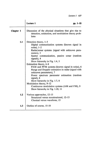
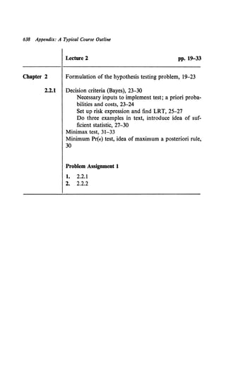
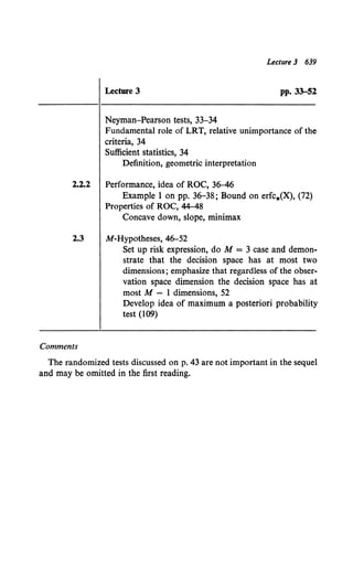
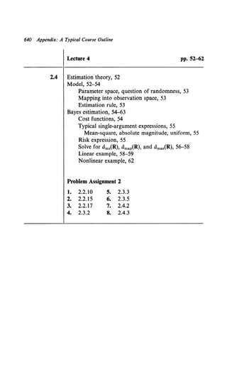
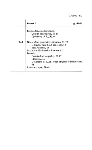
659. Comments
Lecture 7 643
Lecture 7 pp. 98-133
2.6 General Gaussian problem (continued)
Equal covariance matrices, unequal mean vectors, 98-107
Expression for d2, interpretation as distance, 99-100
Diagonalization of Q, eigenvalues, eigenvectors,
101-107
Geometric interpretation, 102
Unequalcovariance matrices,equal meanvectors,107-116
Structure of LRT, interpretation as estimator, 107
Diagonal matrices with identical components, x2
density, 107-111
Computational problem, motivation ofperformance
bounds, 116
2.7 Assignsectiononperformance bounds asreading, 116-133
1. (p. 99} Note that Var[JI H1] = Var[ll H0 ] and that d2 completely
characterizes the test because I is Gaussian on both hypotheses.
2. (p. 119) The idea of a "tilted" density seems to cause trouble.
Emphasize the motivation for tilting.

660. 644 Appendix: A Typical Course Outline
Lecture 8 pp. 166-186
Cbapter 3
3.1, 3.2 Extension of results to waveform observations
Deterministic waveforms
Time-domain and frequency-domain characteriza-
tions, 166-169
Orthogonal function representations, 169-174
Complete orthonormal sets, 171
Geometric interpretation, 172-174
3.3, 3.3.1 Second-moment characterizations, 174-178
Positive definiteness, nonnegative definiteness, and
symmetry of covariance functions, 176-177
3.3.3 Gaussian random processes, 182
Difficulty with usual definitions, 185
Definition in terms of a linear functional, 183
Jointly Gaussian processes, 185
Consequences of definition; joint Gaussian density
at any set of times, 184-185
Problem Assignment 4
1. 2.6.2 Optional
2. 2.6.4. 5. 2.7.1
3. 2.6.8 6. 2.7.2
4. 2.6.10

661. Lecture 9 645
Lecture 9 pp. 178--194
3.3.2 Orthogonal representation for random processes,178-182
3.4, 3.4.1,
3.4.2
Choice of coefficients to minimize mean-square
representation error, 178
Choice of coordinate system, 179
Karhunen-Loeve expansion, 179
Properties of integral equations. 180-181
Analogy with finite-dimensional case in Section 2.6
The following comparison should be made:
Gaussian definition
z = gTx
Symmetry
IG.1 = K;t
Nonnegative
definiteness
xTKx ~ 0
Coordinate system
K4> = A4>
Orthogonality
4>t4>; = slf
Mercer's theorem, 181
z = J:g(u) x(u) du
Kx(t, u) = Kx(U, t)
J:dt J:du x(t) Kx{t, u)
x(u) ~ 0
J:Kx(t, u) rfo(u) du
= Ar/J(t) 0 ;5; t ;5; T
J:rPt(t) cl>t{t) dt = 811
Convergence in mean-square sense, 182
Assign Section 3.4 on integral equation solutions for
reading, 186-194

662. 646 Appendix: A Typical Course Outline
3.4.1
3.4.2
3.4.3
3.4.4
3.4.5
3.4.6-3.7
Comment
Lecture 10 pp. 186-226
Solution of integral equations, 186-196
Basic technique, obtain differential equation, solve,
and satisfy boundary conditions, 186-191
Example: Wiener process, 194-196
White noise and its properties, 196-198
Impulsive covariance function, flat spectrum,
orthogonal representation, 197-198
Optimum linear filter, 198-204
This derivation illustrates variational procedures;the
specific result is needed in Chapter 4; the integral
equation (144) should be emphasized because it
appears in many later discussions; a series solution
in terms of eigenvalues and eigenfunctions is
adequate for the present
Assign the remainder of Chapter 3 for reading; Sections
3.5 and 3.6 are not used in the text (some problems use
the results); Section 3.7 is not needed until Section 4.5
(the discussion of vector processes can be avoided until
Section 6.3, when it becomes essential), 204-226
Problem Assignment S
1. 3.3.1 5. 3.4.4
2. 3.3.6 6. 3.4.6
3. 3.3.19 7. 3.4.8
4. 3.3.22
At the beginning of the derivation on p. 200 we assumed h(t, u) was
continuous. Whenever there is a white noise component in r(t) (143), this
restriction does not affect the performance. When KT(t, u) does not contain
an impulse, a discontinuous filter may perform better. The optimum filter
satisfies (138) for 0 :S u :S T if discontinuities are allowed.

663. Lecture 11 647
Lecture 11 pp.%39-257
Chapter 4
4.1 Physical situations in which detection problem arises
Communication, radar/sonar, 239-246
4.2 Detection of known signals in additive white Gaussian
noise, 246-271
Simple binary detection, 247
Sufficient statistic, reduction to scalar problem, 248
Applicability of ROC in Fig. 2.9 with d2 = 2E/N0 ,
250-251
Lack of dependence on signal shape, 253
General binary detection, 254-257
Coordinate system using Gram-Schmidt, 254
LRT, reduction to single sufficient statistic, 256
Minimum-distance rule; "largest-of" rule, 257
Expression for d2, 256
Optimum signal choice, 257

664. 648 Appendix: A Typical Course Outline
Lecture 12 pp. 257-271
4.2.1 M-ary detection in white Gaussian noise, 257
Set of sufficient statistics; Gram-Schmidt procedure
leads to at most M (less if signals have some linear
dependence); Illustrate with PSK and FSK set, 259
Emphasize equal a priori probabilities and mini-
mum Pr(") criterion. This leads to minimum-
distance rules. Go through three examples in text
and calculate Pr(t)
Example 1 illustrates symmetry and rotation, 261
Example 3 illustrates complexity of exact calcula-
tion for a simple signal set. Derive bound and
discuss accuracy, 261-264
Example 4 illustrates the idea of transmitting
sequences of digits and possible performance
improvements, 264-267
Sensitivity, 267-271
Functional variation and parameter variation; this
is a mundane topic that is usually omitted; it is a
crucial issue when we try to implement optimum
systems and must measure the quantities needed in
the mathematical model
Problem Assignment 6
1. 4.2.4
2. 4.2.6
3. 4.2.8
4. 4.2.9
s. 4.2.16
6. 4.2.23

665. Lecture 13 649
Lecture 13 pp. 271-278
4.2.2 Estimation of signal parameters
Derivation of likelihood function, 274
Necessary conditions on amap(r(t)) and am1
(r(t)), 274
Generalization of Cramer-Rao inequality, 275
Conditions for efficient estimates, 276
Linear estimation, 271-273
Simplicity of solution, 272
Relation to detection problem, 273
4.2.3 Nonlinear estimation, 273-286
Optimum receiver for estimating arrival time
(equivalently, the PPM problem), 276
Intuitive discussion of system performance, 277

666. 650 Appendix: A Typical Course Outline
Lecture 14 pp. 278-289
4.2.3 Nonlinear estimation (continued), 278-286
Pulse frequency modulation (PFM), 278
An approximation to the optimum receiver (interval
selector followed by selection of local maximum),
279
Performance in weak noise, effect of{3Tproduct, 280
Threshold analysis, using orthogonal signal approxi-
mation, 280-281
Bandwidth constraints, 282
Design of system under threshold and bandwidth
constraints, 282
Total mean-square error, 283-285
4.2.4 Summary: known signals in white noise, 286-287
4.3 Introduction to colored noise problem, 287-289
Model, observation interval, motivation for includ-
ing white noise component
Problem Assignment 7
1. 4.2.25 3. 4.2.28
2. 4.2.26
Comments on Lecture 15 (lecture is onp. 651)
1. As in Section 3.4.5, we must be careful about the endpoints of the
interval. If there is a white noise component, we may choose a continuous
g(t) without affecting the performance. This leads to an integral equation
on an open interval. If there is no white component, we must use a closed
interval and the solution will usually contain singularities.
2. On p. 296 it is useful to emphasize the analogy between an inverse
kernel and an inverse matrix.

667. 4.3
4.3.1, 4.3.2,
4.3.3
Lecture 15 651
Lecture 15 pp. 289-333
Colored noise problem
Possible approaches: Karhunen-Loeve expansion,
prewhitening filter, generation of sufficient statistic,
289
Reversibility proof (this idea is used several times in
the text), 289-290
Whitening derivation, 290-297
Define whitening filter, hw(t, u), 291
Define inverse kernel Qn(t, u) and function for cor-
relator g(t), 292
Derive integral equations for above functions, 293-
297
Draw the three realizations for optimum receiver
(Fig. 4.38), 293
Construction of Qn(t, u)
Interpretation as impulse minus optimum linear
filter, 294-295
Series solutions, 296-297
4.3.4 Performance, 301-307
Expression for d2 as quadratic form and in terms of
eigenvalues, 302
Optimum signal design, 302-303
Singularity, 303-305
Importance of white noise assumption and effect of
removing it
4.3.8 Duality with known channel problem, 331-333
4.3.5-4.3.8 Assign as reading,
1. Estimation (4.3.5)
2. Solution to integral equations (4.3.6)
3. Sensitivity (4.3.7)
4. Known linear channels (4.3.8)
Problem Set 7 (continued)
4. 4.3.4 7. 4.3.12
5. 4.3.7 8. 4.3.21
6. 4.3.8

668. 652 Appendix: A Typical Course Outline
Lecture 16 pp. 333-377
4.4 Signals with unwanted parameters, 333-366
Example of random phase problem to motivate the
model, 336
Construction of LRT by integrating out unwanted
parameters, 334
Models for unwanted parameters, 334
4.4.1 Random phase, 335-348
Formulate bandpass model, 335-336
Go to A(r(t)) by inspection, define quadrature
sufficient statistics Lc and L., 337
Introduce phase density (364), motivate by brief
phaselock loop discussion, 337
Obtain LRT, discuss properties ofln l 0(x), point out
it can be eliminated here but will be needed in
diversity problems, 338-341
Compute ROC for uniform phase case, 344
Introduce Marcum's Q function
Discuss extension to binary and M-ary case, signal
selection in partly coherent channels
4.4.2 Random amplitude and phase, 349-366
Motivate Rayleigh channel model, piecewise con-
stant approximation, possibility of continuous
measurement, 349-352
Formulate in terms of quadrature components, 352
Solve general Gaussian problem, 352-353
Interpret as filter-squarer receiver and estimator-
correlator receiver, 354
Apply Gaussian result to Rayleigh channel, 355
Point out that performance was already computed
in Chapter 2
Discuss Rician channel, modifications necessary to
obtainreceiver, relation to partially-coherent channel
in Section 4.4.1, 360-364
4.5--4.7 Assign Section 4.6 to be read before next lecture;
Sections 4.5 and 4.7 may be read later, 366-377

669. Lecture 16 653
Lecture 16 (continued)
Problem Assignment 8
1. 4.4.3 5. 4.4.29
2. 4.4.5 6. 4.4.42
3. 4.4.13 7. 4.6.6
4. 4.4.27

670. 654 Appendix: A Typical Course Outline
Lecture 17 pp. 370-460
4.6 Multiple-parameter estimation, 370-374
Set up a model and derive MAP equations for the
colored noise case, 374
The examples can be left as a reading assignment but
the MAP equations are needed for the next topic
Chapter 5 Continuous waveform estimation, 423-460
5.1, 5.2 Model of problem, typical continuous systems such
as AM, PM, and FM; other problems such as
channel estimation; linear and nonlinear modula-
tion, 423-426
Restriction to no-memory modulation, 427
Definition of dmap(r(t)) in terms of an orthogonal
expansion, complete equivalence to multiple para-
meter problem, 429-430
Derivation of MAP equations (31-33), 427-431
Block diagram interpretation, 432-433
Conditions for an efficient estimate to exist, 439
5.3-5.6 Assign remainder of Chapter 5 for reading, 433-460

671. Chapter 6
6.1
Lecture 18 655
Lecture 18 pp. 467-481
Linear modulation
Model for linear problem, equations for MAP interval
estimation, 467-468
Property I : MAP estimate can be obtained by
using linear processor; derive in-
tegral equation, 468
Property 2: MAP and MMSE estimates coincide
for linear modulation because effi-
cient estimate exists, 470
Formulation of linear point estimation problem, 470
Gaussian assumption, 471
Structured approach, linear processors
Property 3: Derivation of optimum linear pro-
cessor, 472
Property 4: Derivation of error expression [em-
phasize (27)], 473
Property 5: Summary ofinformation needed, 474
Property 6: Optimum error and received wave-
form are uncorrelated, 474
Property 6A: In addition, e0(t) and r(u) are
statistically independent under Gaus-
sian assumption, 475
Optimality of linear filter under Gaussian assumption,
475-477
Property 7: Prove no other processor could be
better, 475
Property 7A: Conditions for uniqueness, 476
Generalization of criteria (Gaussian assumption), 477
Property 8: Extend to convex criteria; unique-
ness for strictly convex criteria;
extend to monotone increasing cri-
teria, 477-478
Relationship to interval and MAP estimators
Property 9: Interval estimate is a collection of
point estimates, 478
Property 10: MAP point estimates and MMSE
point estimates coincide, 479

672. 656 Appendix: A Typical Course Outline
Lecture 18 (continued)
Summary, 481
Emphasize interplay between structure, criteria, and
Gaussian assumption
Point out that the optimum linear filter plays a
central role in nonlinear modulation (Chapter 11.2)
and detection of random signals in random noise
(Chapter 11.3)
Problem Assignment 9
1. 5.2.1 3. 6.1.1
2. 5.3.5 4. 6.1.4

673. Lecture 19 657
Lecture 19 pp. 481-515
6.2 Realizable linear filters, stationary processes, infinite time
(Wiener-Hopf problem)
Modification of general equation to get Wiener-
Hopf equation, 482
Solution of Wiener-Hopf equation, rational spectra, 482
Whitening property; illustrate with one-pole ex-
ample and then indicate general case, 483-486
Demonstrate a unique spectrum factorization pro-
cedure, 485
Express H~(jw) in terms of original quantities;
define "realizable part" operator, 487
Combine to get final solution, 488
Example of one-pole spectrum plus white noise, 488-493
Desired signal is message shifted in time
Find optimum linear filter and resulting error, 494
Prove that the mean-square error is a monotone in-
creasing function ofa, the prediction time; emphasize
importance of filtering with delay to reduce the
mean-square error, 493-495
Unrealizable filters, 496-497
Solve equation by using Fourier transforms
Emphasize that error performance is easy to com-
pute and bounds the performance of a realizable
system; unrealizable error represents ultimate per-
formance; filters can be approximated arbitrarily
closely by allowing delay
Closed-form error expressions in the presence of white
noise, 498-508
Indicate form of result and its importance in system
studies
Assign derivation as reading
Discuss error behavior for Butterworth family, 502
Assign the remainder of Section 6.2 as reading, 508-515
Problem Assignment 9 (continued)
5. 6.2.1 7. 6.2.7
6. 6.2.3 8. 6.2.43

674. 658 Appendix: A Typical Course Outline
Lecture 20* pp. 515-538
6.3 State-variable approach to optimum filters (Kalman-
Bucy problem), 515-575
6.3.1 Motivation for differential equation approach, 515
State variable representation of system, 515-526
Differential equation description
Initial conditions and state variables
Analog computer realization
Process generation
Example 1: First-order system, 517
Example 2: System with poles only, introduction of
vector differential equation, vector block
diagrams, 518
Example 3: General linear differential equation, 521
Vector-inputs, time-varying coefficients, 527
System observation model, 529
State transition matrix, <!>(t, T), 529
Properties, solution for time-invariant case, 529-531
Relation to impulse response, 532
Statistical properties of system driven by white noise
Properties 13 and 14, 532-534
Linear modulation model in presence of white noise, 534
Generalizations of model, 535-538
Problem Assignment 10
1. 6.3.1 4. 6.3.9
2. 6.3.4 5. 6.3.12
3. 6.3.7(a, b) 6. 6.3.16
•Lectures 20--22 may be omitted if time is a limitation and the material in Lectures
28-30 on the radar/sonar problem is of particular interest to the audience. For graduate
students the material in 20-22 should be used because of its fundamental nature and
importance in current research.

675. Lecture 21 659
Lecture 21 PP• 538-546
6.3.2 Derivation of Kalman-Bucy estimation equations
Step 1: Derive the differential equation that
h0 {t, T) satisfies, 539
Step 2: Derive the differential equation that
i(t) satisfies, 540
Step 3: Relate ;p(t), the error covariance
matrix, and b0{t, t), 542
Step 4: Derive the variance equation, 542
Properties of variance equation
Property 15: Steady-state solution, relation to
Wiener filter, 543
Property 16: Relation to two simultaneous linear
vector, equations; analytic solution
procedure for constant coefficient
case, 545

676. 660 Appendix: A Typical Course Outline
Lecture 22 pp. 546-586
6.3.3 Applications to typical estimation problems, 546-566
Example I: One-pole spectrum, transient behavior,
546
Example 3: Wiener process, relation to pole-
splitting, 555
Example 4: Canonic receiver for stationary mes-
sages in single channel, 556
Example 5: FM problem; emphasize that optimum
realizable estimation commutes with
linear transformations, not linear filter-
ing (this point seems to cause confusion
unless discussed explicitly), 557-561
Example 7: Diversity system, maximal ratio com-
bining, 564-565
6.3.4 Generalizations, 566-575
List the eight topics in Section 6.3.4 and explain
why they are of interest; assign derivations as
reading
Compare state-variable approach to conventional
Wiener approach, 575
6.4 Amplitude modulation, 575-584
Derive synchronous demodulator; assign the re-
mainder of Section 6.4 as reading
6.5-6.6 Assign remainder of Chapter 6 as reading. Emphasize
the importance of optimum linear filters in other areas
Problem Assignment 11
1. 6.3.23 4. 6.3.37
2. 6.3.27 s. 6.3.43
3. 6.3.32 6. 6.3.44

677. Chapter fl-2
11-2.2
fl-2.3
Lecture 23 661
Lecture 23*
Nonlinear modulation
Model of angle modulation system
Applications; synchronization, analog communica-
tion
Intuitive discussion of what optimum demodulator
should be
MAP estimation equations
DerivedinChapter1-5,specializetophasemodulation
Interpretation as unrealizable block diagram
Approximation by realizable loop followed by
unrealizable postloop filter
Derivation of linear model, loop error variance
constraint
Synchronization example
Design of filters
Nonlinear behavior
Cycle-skipping
Indicate method of performing exact nonlinear
analysis
*The problem assignments for Lectures 23-32 will be included in Appendix 1 of Part II.

678. 662 Appendix: A Typical Course Outline
Lecture 24
IT-2.5 Frequency modulation
Design of optimum demodulator
Optimum loop filters and postloop filters
Signal-to-noise constraints
Bandwidth constraints
Indicate comparison of optimum demodulator and
conventional limiter-discriminator
Discuss other design techniques
IT-2.6 Optimum angle modulation
Threshold and bandwidth constraints
Derive optimum pre-emphasis filter
Compare with optimum FM systems

679. Lecture 25 663
Lecture 25
11-2.7 Comparison of various systems for transmitting analog
messages
Sampled and quantized systems
Discuss simple schemes such as binary and M-ary
signaling
Derive expressions for system transmitting at
channel capacity
Sampled, continuous amplitude systems
Develop PFM system, use results from Chapter 1-4,
and compare with continuous FM system
Bounds on analog transmission
Rate-distortion functions
Expression for Gaussian sources
Channel capacity formulas
Comparison for infinite-bandwidth channel of
continuous modulation schemes with the bound
Bandlimited message and bandlimited channel
Comparison of optimum FM with bound
Comparison of simple companding schemes with
bound
Summary ofanalog message transmission and continuous
waveform estimation

680. 664 Appendix: A Typical Course Outline
Lecture 26
Chapter ll-3 Gaussian signals in Gaussian noise
3.2.1 Simple binary problem, white Gaussian noise on H0 and
H1o additional colored Gaussian noise on H1
Derivation of LRT using Karhunen-Loeve expan-
sion
Various receiver realizations
Estimator-correlator
Filter-squarer
Structure with optimum realizable filter as com-
ponent (this discussion is most effective when
Lectures 20-22 are included; it should be men-
tioned, however, even if they were not studied)
Computation of bias terms
Performance bounds using J.L(S) and tilted probability
densities (at this point we must digress and develop the
material in Section 2.7 of Chapter I-2).
Interpretation of J.L(s) in terms of realizable filtering
errors
Example: Structure and performance bounds for
the case in which additive colored noise
has a one-pole spectrum

681. Lecture 27 665
Lecture 27
3.2.2 General binary problem
Derive LRT using whitening approach
Eliminate explicit dependence on white noise
Singularity
Derive tL(s) expression
Symmetric binary problems
Pr(~-) expressions, relation to Bhattacharyya distance
Inadequacy of signal-to-noise criterion

682. 666 Appendix: A Typical Course Outline
Lecture 28
Chapter ll-3 Special cases of particular importance
3.2.3 Separable kernels
Time diversity
Frequency diversity
Eigenfunction diversity
Optimum diversity
3.2.4 Coherently undetectable case
Receiver structure
Show how p.(s) degenerates into an expression in-
volving d2
3.2.5 Stationary processes, long observation times
Simplifications that occur in receiver structure
Use the results in Lecture 26 to show when these
approximations are valid
Asymptotic formulas for p.(s)
Example: Do same example as in Lecture 26
Plot Pv versus kT for various E/N0 ratios and
P/s
Find the optimum kT product (this is continuous
version of the optimum diversity problem)
Assign remainder of Chapter II-3 (Sections 3.3-3.6) as
reading

683. Lecture 29 667
Lecture 29
Chapter ll-4 Radar-sonar problem
4.1 Representation of narrow-band signals and processes
Typical signals, quadrature representation, complex
signal representation. Derive properties: energy,
correlation, moments; narrow-band random pro-
cesses; quadrature and complex waveform repre-
sentation. Complex state variables
Possible target models; develop target hierarchy in Fig.
4.6
4.2 Slowly-fluctuating point targets
System model
Optimum receiver for estimating range and Doppler
Develop time-frequency autocorrelation function
and radar ambiguity function
Examples: Rectangular pulse
Ideal ambiguity function
Sequence of pulses
Simple Gaussian pulse
Effect of frequency modulation on the signal
ambiguity function
Accuracy relations

684. 668 Appendix: A Typical Course Outline
Lecture 30
4.2.4 Properties of autocorrelation functions and ambiguity
functions. Emphasize:
Property 3: Volume invariance
Property 4: Symmetry
Property 6: Scaling
Property 11 : Multiplication
Property 13: Selftransform
Property 14: Partial volume invariances
Assign the remaining properties as reading
4.2.5 Pseudo-random signals
Properties of interest
Generation using shift-registers
4.2.6 Resolution
Model of problem, discrete and continuous resolu-
tion environments, possible solutions: optimum or
"conventional" receiver
Performance of conventional receiver, intuitive dis-
cussion of optimal signal design
Assign the remainder of Section 4.2.6 and Section 4.2.7
as reading.

685. Lecture 31 669
Lecture 31
4.3 Singly spread targets (or channels)
Frequency spreading-delay spreading
Model for Doppler-spread channel
Derivation of statistics (output covariance)
Intuitive discussion of time-selective fading
Optimum receiver for Doppler-spread target (simple
example)
Assign the remainder of Section 4.3 as reading
Doubly spread targets
Physical problems of interest: reverberation, scatter
communication
Model for doubly spread return, idea of target or
channel scattering function
Reverberation (resolution in a dense environment)
Conventional or optimum receiver
Interaction between targets, scattering function, and
signal ambiguity function
Typical target-reverberation configurations
Optimum signal design
Assign the remainder of Chapter II-4 as reading

686. 670 Appendix: A Typical Course Outline
Lecture 32
Chapter ll-5
5.1 Physical situations in which multiple waveform and
multiple variable problems arise
Review vector Karhunen-Loeve expansion briefly (Chap-
ter 1-3)
5.3 Formulate array processing problem for sonar
5.3.1 Active sonar
Consider single-signal source, develop array steering
Homogeneous noise case, array gain
Comparison of optimum space-time system with
conventional space-optimum time system
Beam patterns
Distributed noise fields
Point noise sources
5.3.2 Passive sonar
Formulate problem, indicate result. Assign deriva-
tion as reading
Assign remainder of Chapter 11-5 and Chapter 11-6 as
reading

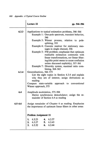
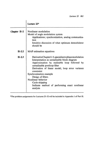
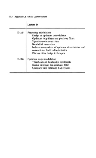
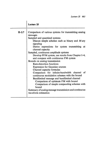
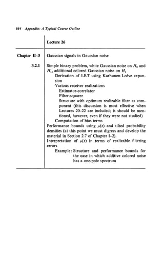
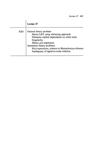
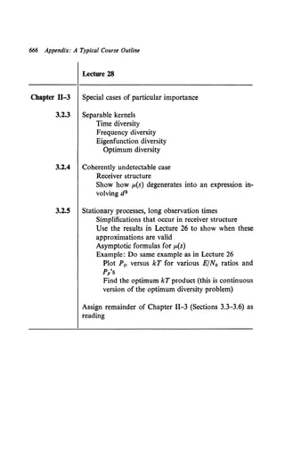
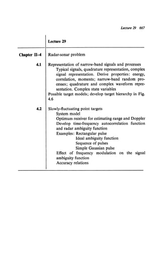
687. Detection, Estimation, and Modulation Theory, Part I:
Detection, Estimation, and Linear Modulation Theory. Harry L. Van Trees
Copyright © 2001 John Wiley & Sons, Inc.
ISBNs: 0-471-09517-6 (Paperback); 0-471-22108-2 (Electronic)
Glossary
In this section we discuss the conventions, abbreviations, and symbols
used in the book.
CONVENTIONS
The following conventions have been used:
I. Boldface roman denotes a vector or matrix.
2. The symbol I I means the magnitude of the vector or scalar con-
tained within.
3. The determinant of a square matrix A is denoted by IAI or det A.
4. The script letters 3'( ·) and C(·) denote the Fourier transform and
Laplace transform respectively.
5. Multiple integrals are frequently written as,
that is, an integral is inside all integrals to its left unless a multiplication is
specifically indicated by parentheses.
6. E[ ·] denotes the statistical expectation of the quantity in the bracket.
The overbar xis also used infrequently to denote expectation.
7. The symbol ® denotes convolution.
x(t)® y(t) ~ J_"'"' x(t - -r)y(-r) d-r
8. Random variables are lower case (e.g., x and x). Values of random
variables and nonrandom parameters are capital (e.g., X and X). In some
estimation theory problems much of the discussion is valid for both ran-
dom and nonrandom parameters. Here we depart from the above con-
ventions to avoid repeating each equation.
671

688. 672 Glossary
9. The probability density of x is denoted by Px(·) and the probability
distribution by PxC·). The probability of an event A is denoted by Pr[A].
The probability density of x, given that the random variable a has a value
A, is denoted by Px 1a(XIA). When a probability density depends on non-
random parameter A we also use the notation Px1a(XIA). {This is non-
standard but convenient for the same reasons as 8.)
10. A vertical line in an expression means "such that" or "given that";
that is Pr[Aix ~ X] is the probability that event A occurs given that the
random variable x is less than or equal to the value of X.
11. Fourier transforms are denoted by both FUw) and F(w). The latter
is used when we want to emphasize that the transform is a real-valued
function of w. The form used should always be clear from the context.
12. Some common mathematical symbols used include,
(i) oc proportional to
(ii) t- r- t approaches T from below
A orB or both
(iii) A+ B~A u B
(iv) l.i.m. limit in the mean
(v) J:al dR an integral over the same dimension as the
vector
(vi) AT
(vii) A-l
(viii) 0
(ix) (~)
(x) ~
transpose of A
inverse of A
matrix with all zero elements
b. . 1 ffi . ( N! )
momta coe ctent = k! (N _ k)!
defined as
(xi) fndR integral over the set .Q
ABBREVIATIONS
Some abbreviations used in the text are:
ML
MAP
PPM
PAM
PM
DSB-SC-AM
DSB-AM
maximum likelihood
maximum a posteriori probability
pulse frequency modulation
pulse amplitude modulation
frequency modulation
double-sideband-suppressed carrier-amplitude modula-
tion
double sideband-amplitude modulation

689. PM
NLNM
FM/FM
MMSE
ERB
UMP
ROC
LRT
SYMBOLS
phase modulation
nonlinear no-memory
two-level frequency modulation
minimum mean-square error
equivalent rectangular bandwidth
uniformly most powerful
receiver operating characteristic
likelihood ratio test
Glossary 673
The principal symbols used are defined below. In many cases the vector
symbol is an obvious modification ofthe scalar symbol and is not included.
Aa
A,
ii(t)
Oabs
dmap
ami
aml(t)
Oms
a:
a
a:
B
B(A)
Ba(t)
fJ
c
C(a,)
C(a, a)
C(d.(t))
CF
c,i
eM
Coo
C(t)
Ca(t)
actual value of parameter
sample at t1
Hilbert transform of a(t)
minimum absolute error estimate of a
maximum a posteriori probability estimate of a
maximum likelihood estimate of A
maximum likelihood estimate of a(t)
minimum mean-square estimate of a
amplitude weighting of specular component in Rician
channel
constraint on PF (in Neyman-Pearson test)
delay or prediction time (in context of waveform
estimation)
constant bias
bias that :s a function of A
matrix in state equation for desired signal
parameter in PFM and angle modulation
channel capacity
cost of an estimation error, a,
cost of estimating a when a is the actual parameter
cost function for point estimation
cost of a false alarm (say H1 when H0 is true)
cost of saying H, is true when H1 is true
cost of a miss (say H0 when H1 is true)
channel capacity, infinite bandwidth
modulation (or observation) matrix
observation matrix, desired signal

690. 674 Glossary
CM(t)
CN(t)
X
Xa
Xo
x2
J
d(t)
d(t)
da
JB(t)
d,
Jo(t)
d.(t, a(t))
dE(f)
d.(t)
8
!::.
!::.d
!::.dx
!::.N
!::.n
am
4Q
E
message modulation matrix
noise modulation matrix
parameter space
parameter space for a
parameter space for 8
chi-square (description of a probability density)
denominator of spectrum
desired function of parameter
performance index parameter on ROC for Gaussian
problems
estimate of desired function
desired signal
estimate of desired signal
actual performance index
Bayes point estimate
parameter in FM system (frequency deviation)
optimum MMSE estimate
derivative of s(t, a(t)) with respect to a(t)
error in desired point estimate
output of arbitrary nonlinear operation
phase of specular component (Rician channel)
interval in PFM detector
change in performance index
desired change in d
change in white noise level
constraint on covariance function error
mean difference vector (i.e., vector denoting the dif-
ference between two mean vectors)
matrix denoting difference between two inverse co-
variance matrices
energy (no subscript when there is only one energy in
the problem)
expectation over the random variable a only
energy in error waveform (as a function of the number
of terms in approximating series)
energy in interfering signal
energy on ith hypothesis
expected value of received energy
transmitted energy
energy in y(t)

691. EJ
ET
erf (·)
err.(·)
erfc (·)
erfc* ( ·)
7J
E(·)
F
f(t)
f(t)
f(t: r(u),
T.. :s; u :s; T1)
fc
ft:.(t)
F
F(t)
Fa(t)
g(t)
g(t, A), g(t, A)
g(.,)
gh(t)
g,(T)
g10(T), G10Uw)
gpu(T)
gpuo(T), GpuoUw}
g6(t)
gt:.(t)
g~
goo(t), GooUw)
Glossary 675
energy of signals on H1 and H0 respectively
energy in error signal (sensitivity context)
error waveform
interval error
total error
error function (conventional)
error function (as defined in text)
complement of error function (conventional)
complement of error function (as defined in text)
(eta) threshold in likelihood ratio test
expectation operation (also denoted by ( ·) infrequently)
function to minimize or maximize that includes
Lagrange multiplier
envelope of transmitted signal
function used in various contexts
nonlinear operation on r(u) (includes linear operation
as special case)
oscillator frequency (w. = 2Tr/c)
normalized difference signal
matrix in differential equation
time-varying matrix in differential equation
matrix in equation describing desired signal
factor of S1( w) that has all of the poles and zeros in
LHP (and t of the zeros on jw-axis). Its transform is
zero for negative time.
function in colored noise correlator
function in problem of estimating A (or A) in colored
noise
a function of an eigenvalue
homogeneous solution
filter in loop
impulse response and transfer function optimum loop
filter
unrealizable post-loop filter
optimum unrealizable post-loop filter
impulse solution
difference function in colored noise correlator
a weighted sum of g(.1)
infinite interval solution

692. 676 Glossary
G
G(t)
G"
Ga(t)
g(t)
g..(A)
r(x)
')I
')I
Ya
H 0 , H 1, .•• , H1
h(t, u)
hch(t, u)
hL(t)
h.(t, u)
h~(T), H~Uw)
hw(t, u)
h((t, u)
h.(t, u)
H
h.(t, u)
J(t, u)
J!i
J- 1(t, u)
Jij
JK(t, u)
J
Jv
Jp
matrix in differential equation
time-varying matrix in differential equation
linear transformation describing desired vector d
matrix in differential equation for desired signal
function for vector correlator
nonlinear transformation describing desired vector d
Gamma function
parameter (y = kvT+i)
threshold for arbitrary test (frequently various constants
absorbed in y)
factor in nonlinear modulation problem which controls
the error variance
hypotheses in decision problem
impulse response of time-varying filter (output at t due
to impulse input at u)
channel impulse response
low pass function (envelope of bandpass filter)
optimum linear filter
optimum processor on whitened signal: impulse
response and transfer function, respectively
optimum unrealizable filter (impulse response and
transfer function)
whitening filter
arbitrary linear filter
linear filter in uniqueness discussion
linear matrix transformation
optimum linear matrix filter
modified Bessel function of 1st kind and order zero
integrals
incomplete Gamma function
identity matrix
information kernel
elements in J-1
inverse information kernel
elements in information matrix
kth term approximation to information kernel
information matrix (Fisher's)
data component of information matrix
a priori component of information matrix

693. Kna(t, u)
Kne(t, u)
Kn.(t, u)
Kx(t, u)
k
k(t, r(u))
K
ka(t)
ka(t, v)
I(R), I
I(A)
Ia
fc, /8
I
A
A(R)
A(rK(t))
A(rK(t), A)
AB
Aer
Ag
Am
A3ctb
Ax
1.x(t)
,
At
~ch
>.l
In
loga
total information matrix
transform of J(-r)
transform of J- 1(-r)
Glossary 677
actual noise covariance (sensitivity discussion)
effective noise covariance
error in noise covariance (sensitivity discussion)
covariance function of x(t)
Boltzmann's constant
operation in reversibility proof
covariance matrix
linear transformation of x(t)
matrix filter with p inputs and q outputs relating a(v)
and d(t)
matrix filter with p inputs and n outputs relating a(v)
and x(u)
sufficient statistic
likelihood function
actual sufficient statistic (sensitivity problem)
sufficient statistics corresponds to cosine and sine com-
ponents
a set of sufficient statistics
a parameter which frequently corresponds to a signal-
to-noise ratio in message ERB
likelihood ratio
likelihood ratio
likelihood function
signal-to-noise ratio in reference bandwidth for
Butterworth spectra
effective signal-to-noise ratio
generalized likelihood ratio
parameter in phase probability density
signal-to-noise ratio in 3-db bandwidth
covariance matrix of vector x
covariance matrix of state vector ( = Kx(t, t))
Lagrange multiplier
eigenvalue of matrix or integral equation
eigenvalues of channel quadratic form
total eigenvalue
natural logarithm
logarithm to the base a

694. 678 Glossary
MxUv), MxUv)
mx(t)
M
m
/L(S)
N
N
N(m, o)
N(w2)
Nee
No
n(t)
n.(t)
nEI(t)
n,
nRI(t)
n.(t)
ii••(t)
ficu(t)
N
n,n
ea.
~I
~IJ(t)
~ml
~p(t)
~p,(t)
~Pnlt)
~~n
~P«J
~u
gun
~.(t)
~ac
~a(t)
~P«J
characteristic function of random variable x (or x)
mean-value function of process
matrix used in colored noise derivation
mean vector
exponent of moment-generating function
dimension of observation space
number of coefficients in series expansion
Gaussian (or Normal) density with mean m and stan-
dard deviation a
numerator of spectrum
effective noise level
spectral height Uoules)
noise random process
colored noise (does not contain white noise)
external noise
ith noise component
receiver noise
noise component at output of whitening filter
MMSE realizable estimate of colored noise component
MMSE unrealizable estimate of colored noise com-
ponent
noise correlation matrix numbers)
noise random variable (or vector variable)
cross-correlation between error and actual state vector
expected value of interval estimation error
elements in error covariance matrix
variance of ML interval estimate
expected value of realizable point estimation error
variance of error of point estimate of ith signal
normalized realizable point estimation error
normalized error as function of prediction (or lag) time
expected value of point estimation error, statistical
steady state
optimum unrealizable error
normalized optimum unrealizable error
mean-square error using nonlinear operation
actual covariance matrix
covariance matrix in estimating d(t)
steady-state error covariance matrix

695. p
Pr(e)
PD
Pee
PF
PI
PM
PD(8)
p
Po
Pr!H,(RIHI)
Px1(Xt) or
Px1(X: t)
cp(t)
cPt(t)
cfox(s)
cf,(t)
.PL(t)
P(t)
~(t, T)
~(t- t0)~~(T)
Pr[ ·], Pr( ·)
Q(a, {3)
Qn(t, u)
q
Q
R
Rx(t, u)
.1t
.1t(d(t), t)
.1tabs
j{,B
carrier frequency (radians/second)
Doppler shift
power
probability of error
Glossary 679
probability of detection (a conditional probability)
effective power
probability of false alarm (a conditional probability)
a priori probability of ith hypothesis
probability of a miss (a conditional probability)
probability of detection for a particular value of 8
operator to denote d/dt (used infrequently)
fixed probability of interval error in PFM problems
probability density of r, given that H1 is true
probability density of a random process at time t
eigenfunction
ith coordinate function, ith eigenfunction
moment generating function of random variable x
phase of signal
low pass phase function
cross-correlation matrix between input to message
generator and additive channel noise
state transition matrix, time-varying system
state transition matrix, time-invariant system
probability of event in brackets or parentheses
Marcum's Q function
inverse kernel
height of scalar white noise drive
covariance matrix of vector white noise drive (Section
6.3)
inverse of covariance matrix K
inverse of covariance matrix K1, K0
inverse matrix kernel
rate (digits/second)
correlation function
risk
risk in point estimation
risk using absolute value cost function
Bayes risk

696. 680 Glossary
rc(t)
rg(l)
rx(t)
'*(t)
r*a(t)
r**(t)
Pii
P12
R(t)
R
SUw)
Sc(w)
Son[·, ·]
SQ(w)
Sr(w)
Sx(w)
s••Uw)
s(t)
s(t, A)
s(t, a(t))
Sa(l)
s1(t)
Sla(t)
s1
S;
Sr(t, 8)
St(t)
so(t)
s1(t)
s1(t, 8), s0(t, 8)
s,(t)
risk using fixed test
risk using mean-square cost function
risk using uniform cost function
received waveform (denotes both the random process
and a sample function of the process)
combined received signal
output when inverse kernel filter operates on r(t)
K term approximation
output of whitening filter
actual output of whitening filter (sensitivity context)
output of SQ(w) filter (equivalent to cascading two
whitening filters)
normalized correlation s1(t) and sJCt) (normalized signals)
normalized covariance between two random variables
covariance matrix of vector white noise w(t)
correlation matrix of errors
error correlation matrix, interval estimate
observation vector
radial prolate spheroidal function
Fourier transform of s(t)
spectrum of colored noise
angular prolate spheroidal function
Fourier transform of Q(T)
power density spectrum of received signal
power density spectrum
transform of optimum error signal
signal component in r(t), no subscript when only one
signal
signal depending on A
modulated signal
actual s(t) (sensitivity context)
interfering signal
actual interfering signal (sensitivity context)
coefficient in expansion of s(t)
ith signal component
received signal component
signal transmitted
signal on H0
signal on H1
signal with unwanted parameters
error signal (sensitivity context)

697. st>(t)
sn(t)
s,*(t)
s*(t)
s*.(t)
T.
o, e
{j
Oa
ocb(t)
81
T(t, T)
[ )T
u_1(t)
u(t), u(t)
v
vcb(t)
v(t)
v1(t), v2(t)
w
WUw)
Wch
w-1Uw)
w(t)
W(T)
w
x(t)
x(t)
x(t)
X
x(t)
Xa(t)
difference signal ('VE1 s1(t) - v'Eo s0(t))
random signal
whitened difference signal
Glossary 681
signal component at output of whitening filter
output of whitening filter due to signal error
variance
variance on H1, H 0
error variance
vector signal
effective noise temperature
unwanted parameter
phase estimate
actual phase in binary system
phase of channel response
estimate of 81
transition matrix
transpose of matrix
unit step function
input to system
variable in piecewise approximation to Vch(t)
envelope of channel response
combined drive for correlated noise case
vector functions in Property 16 of Chapter 6
bandwidth parameter (cps)
transfer function of whitening filter
channel bandwidth (cps) single-sided
transform of inverse of whitening filter
white noise process
impulse response of whitening filter
a matrix operation whose output vector has a diagonal
covariance matrix
input to modulator
random process
estimate of random process
random vector
state vector
augmented state vector

698. 682 Glossary
Xac
x11(t)
x1(t)
xM(t)
y(t)
y(t)
y(t)
y
y = s(A)
z
Zc(w)
z.(w)
zloz2
z(t)
z(t)
actual state vector
state vector for desired operation
prefiltered state vector
state vector, message
state vector in model
state vector, noise
output of differential equation
portion of r(t) not needed for decision
transmitted signal
vector component of observation that is not needed for
decision
nonlinear function of parameter A
observation space
integrated cosine transform
integrated sine transform
subspace of observation space
output of whitening filter
gain matrix in state-variable filter (~h0(t, t))

699. Detection, Estimation, and Modulation Theory, Part I:
Detection, Estimation, and Linear Modulation Theory. Harry L. Van Trees
Copyright © 2001 John Wiley & Sons, Inc.
ISBNs: 0-471-09517-6 (Paperback); 0-471-22108-2 (Electronic)
Author Index
Chapter and reference numbers are in brackets; page numbers follow.
Abend, K., [7-57], 629
Abramovitz, M., [2-3), 37, 109
Abramson, N., [7-7], 627; [7-8], 627, 628
Akima, H., [4-88), 278
Algaz~ V. R., [4-67], 377; [7-51], 629
Amara, R. C., [6-12], 511
Arthurs, E., [4-72], 383, 384, 399, 406
Athans, M., [6-26], 517; [7-74), 629
Austin, M., [7-9], 628
Baggeroer, A. B., [3-32], 191; [3-33],
191; [6-36), 552; [6-40]' 567; [6-43)'
573; [6-52], 586; [6-53], 505; [6-54],
586; [7-1]' 624; [7-71]' 629
Baghdady, E. J., [4-17], 246
Balakrishnan, A. V., [4-70], 383; [7-8),
627, 628
Balser, M., [4-51], 349
Barankin, E. W., [2-15], 72, 147
Bartlett, M. S., [3-28), 218
Battin, R. H., [3-11), 187; [4-54), 316
Baumert, L. D., [4-19), 246, 265
Bayes, T., [P-1), vii
Belenski, J. D., (7-65], 629
Bellman, R. E., [2-16), 82, 104; [6-30),
529
Bennett, W. R., [4-92], 394
Berg, R. S., [7-67), 629
Berlekamp, E. R., [2-25], 117,122
Bharucha-Reid, A. T., [2-2], 29
Bhattacharyya, A., [2-13), 71; [2-29), 127
Birdsall, T. G., [4-9], 246; [7-11], 628
Blasbalg, H., [7-13], 628
Bode, H. W., [6-3], 482
Booton, R. C., (6-46], 580
Boyd, D., [7-49], 628
Braverman, D., [7-8), 627, 628
Breipohl, A. M., [7-34), 628
Brennan, D. G., [4-58], 360; [4-65], 369
Brockett, R., [6-13], 511
Bryson, A. E., [6·41], 570, 573; [6-56],
612
Bucy, R. S., [6-23), 516, 543, 557, 575
Bullington, K., [4-52], 349
Bussgang, J. J., [4-82), 406; [7-12), 628;
[7-20]' 628
Cahn, C. R., [4-73), 385; [6-5), 498
Chang, T. T., [5-3], 433
Chernoff, H., [2-28], 117,121
Chu, L. J., [3-19], 193
Close, C. M., [6-27], 516, 529, 599, 600,
609
Coddington, E. A., [6-29), 529
Coles, W. J., [6·35), 543
Collins, L. D., [4-74], 388; [4-79), 400;
[4-91). 388; [6-42)' 570; [6-43]' 573;
[6-53]' 505
Corbato, F. J., [3·19), 193
Costas, J. P., [6-50], 583
Courant, R., [3·3), 180; [4-33), 314, 315
Cramer, H., [2·91, 63, 66, 71, 79, 146
Cruise, T. J., [7-63], 629; [7·76], 629
Daly, R. F., [7-31], 628
Darlington, S., (3-12], 187; (4-62), 316;
[4-87], 278
683

700. 684 Author Index
Davenport, W. B., [P-8], vii; [2-1], 29,
77; [3-1], 176, 178, 179, 180, 187, 226,
227; [4-2]' 240, 352, 391
Davies, I. L., [4-7], 246
Davis, M. C., [6-14], 511
Davisson, L. D., [7-45], 628
DeRusso, P. M., [6-27], 516, 529, 599,
600, 603
DeSoer, C. A., [6-24], 516, 517
DiDonato, A. R., [4-49] , 344
DiToro, M. J., [7-44], 628
Doelz, M., [4-81], 406
Dolph, C. L., [6-22], 516
Dugue, D., [2-31], 66
Durkee, A. L., [4-52], 349
Dym, H., [4-72], 383, 384, 385, 399, 406
Easterling, M. F., [4-19] , 246, 265
Eden, M., [7-8], 627, 628
Ekre, H., [7-29], 628
Elias, P., [7-7], 627
Erdelyi, A., [4-75], 412
Esposito, R., [7-42], 628
Falb, P. L., [6-26], 516
Fano, R. M., [2-24], 117; [4-66], 377;
[7-3]' 627
Faraone, J. N., [7-56], 629
Feigenbaum, E. A., [7-8], 627, 628
Feldman, J. R., [7-56], 629
Feller, w., [2-30], 39; (2-33], 124
Fisher, R. A., [P-4], vii; [2-5], 63; [2-6],
63, 66; (2-7]' 63; [2-8]' 63; [2-19]'
109
Flammer, C., [3-18], 193
Fox, W. C., [4-9], 246; [7-11], 628
Fraser, D. A. S., [7-23], 628
Frazier, M., [6-56], 612
Friedland, B., (6-28], 516, 529
Gagliardi, R. M., [7-17], 628
Gallager, R. G., [2-25], 117, 122; [2-26],
117; [7-4], 627
Galtieri, C. A., [4-43], 301
Gauss, K. F., [P-3], vii
Gill, A., [7-7], 627
Glaser, E. M., [7-48], 628
Gnedenko, B. V., [3-27], 218
Goblick, T. J., [2-35], 133
Goldstein, M. H., [6-46], 580
Golomb, S. W., [4-19], 246, 265; [7-6],
627
Gould, L. A., [6-9], 508
Gray, D., [7-75], 629
Green, P. E., [7-58], 629
Greenwood, J. A., [2-4], 37
Grenander, U., [4-5], 246; [4-30], 297,
299
Groginsky, H. L., [7-39], 628
Guillemin, E. A., [6-37], 548
Gupta, S. C., [6-25], 516
Hahn, P., [4-84], 416
Hajek, J., [4-41], 301
Hancock, J. C., [4-85], 422; [7-43], 628
Harman, W. W., [4-16], 246
Hartley, H. 0., [2-4], 37
Heald, E., [4-82], 406
Helstrom, C. E., [3-13], 187; [3-14], 187;
[4-3], 319; [4-14], 246, 314, 366, 411;
[4-77]' 399; [6-7], 498; [7-18]' 628
Henrich, C. J., [5-3], 433
Hildebrand, F. B., (2-18], 82, 104; [3-31],
200
Hilbert, D., [3-3], 180; [4-33], 314, 315
Ho, Y. C., [7-40], 628
Horstein, M., [7-62], 629
Hsieh, H. C., [6-17], 511
Huang, R. Y., [3-23], 204
Inkster, W. J., [4-52], 349
Jackson, J. L., (6-4], 498
Jacobs, I. M., [2-27], 117; [4-18], 246,
278, 377, 380, 397, 402, 405; [4-86]
416; [7-2]' 627
Jaffe, R., [6-51], 585
Jakowitz, C. V., [7-47], 628
Jarnagin, M. P., [4-49], 344
Johansen, D. E., [4-50], 344; [6-41], 570
573
Johnson, R. A., [3-23], 204
Kadota, T. T., [4-45], 301
Kailath, T., [3-35], 234; [4-32], 299;
[7-8], 627, 628; [7-60], 629
Kaiser, J. F., [6-9], 508
Kalman, R. E., [2-38], 159; [6-23], 516,
543, 557, 575
Kanefsky, M., [7-27], 628; [7-30], 628
Karhunen, K., [3-25], 182
Kavanaugh, R. J., [6-15], 511
Kelly, E. J., [3-24], 221, 224; [4-31],
297, 299

701. Kendall, M. G., [2-11), 63, 149; [7-24),
628
Kendall, W., [7-19], 628
Kolmogoroff, A., [P-6], vii; [6-2], 482
Koschmann, A. H., [7-34], 628
Kotelinikov, V. A., [4-12), 246; [4-13),
246, 278, 286
Krakauer, C. S., [7-68], 629
Kurz, L., [7-32], 628; [7-53], 628
Landau, H. J., [3-16), 193, 194; [3-17],
193, 194; [4-71], 383
Laning, J. H., [3-11], 187; [4-54], 316
Lawson, J. L., [4-6], 246
Lawton, J. G., [5-2], 433; [5-3], 433;
[7-35)' 628
Lee, H. C., [6-19], 511
Lee, R. C., [7-40], 628
Legendre, A. M., [P-2], vii
Lehmann, E. L., [2-17), 92; [7-25], 628
Leondes, C. T., [6-17], 511
Lerner, R. M., [4-67], 377; [7-8], 627,
628; [7-51), 629; [7-54], 629; [7-66),
629
Levin, J. J., [6-32), 543, 545
Levinson, N., [6-29], 529
Lindsey, W. C., [4-85], 422; [4-89), 416;
[6-8], 620
Little, J. D., [3-19], 193
Loeve, M., [3-26], 182; [3-30], 182
Lovitt, W. V., [3-5], 180; [4-34), 314
Lucky, R. W., [7-36], 628
McCracken, L. G., (6-18), 511
McLachlan, N. W., [6-31], 543
McNicol, R. W. E., [4-57), 360
Magill, D. T., (7-37], 628
Mallinckrodt, A. J., [4-25], 286
Manasse, R., [4-26), 286
Marcum, J., [4-46], 344, 412; [4-48],344
Marcus, M. B., [7-14), 628; [7-20], 628
Martin, D., [4-81], 406
Masonson, M., [4-55], 356
Massani, P., [6-16], 511
Massey, J., [7-8], 627, 628
Middleton, D., [3-2], 175; [4-10], 246;
[4-47], 246, 316, 394; [7-12]' 628;
[7-39]' 628, [7-42]' 628; [7-55]' 629
Millard, J. B., [7-32], 628
Miller, K. S., [4-36), 316
Author Index 685
Mohajeri, M., [4-29], 284; [6-20], 595
Morse, P.M., [3-19], 193
Mueller, G. E., [7-8), 627, 628
Mullen, J. A., [7-42], 628
Nagy, B., [3-4], 180
Newton, G. C., [6-9), 508
Neyman, J., [P-5], vii
Nichols, M. H., [5-8], 448
Nolte, L. W., [7-41), 268
North, D. 0., [3-34], 226; [4-20], 249
Nyquist, H., [4-4], 244
Omura, J. K., [7-59], 629; [7-72], 629
Papoulis, A., [3-29], 178; [6-55], 587,
588
Parzen, E., [3-20], 194; [4-40], 301
Pearson, E. S., [P-5], vii
Pearson, K., [2-21], 110; [2-37], 151
Peterson, W. W., [4-9], 246; [7-5], 627;
(7-8], 627, 628; [7-11]' 628
Philips, M. L., [4-58], 360
Pierce, J. N., [2-22], 115; [4-80), 401
Pollak, H. 0., [3-15], 193, 194, 234;
[3-16], 193, 194; [3-17), 193, 194
Price, R., [4-59], 360; [7-7], 627; [7-8],
627, 628
Proakis, J. G., [4-61), 364; [4-83), 406
Ragazzini, J. R., [3-22], 187; [4-35),
316, 319
Rao, C. R., (2-12), 66
Rauch, L. L., [5-5), 433; [5-6], 433;
[5-8]' 448
Rechtin, E., [6-51], 585
Reed, I. S., [4-31), 297, 299; [7-17],628;
[7-19]' 628; [7-21]' 628
Reid, W. T., (6-33), 543; [6-34], 543
Reiffen, B., [4-68], 377; [7-52], 629
Rice, S. 0., [3-7), 185; (4-60), 361
Riesz, F., [3-4), 180
Root, W. L., [P-8), viii; [2-1], 29, 77;
[3-1]' 176, 178, 179, 180, 187, 226,
227; [3-24), 221, 224; [4-2), 240, 352,
391; [4-31]' 297, 299; [4-42], 327
Rosenblatt, F., [3-21], 194
Roy, R. J., [6-27], 516, 529, 599, 600,
603

702. 686 Author Index
Savage, I. R., (7-26], 628
Schalkwijk, J. P. M., [7-60), 629; [7-61),
629
Schwartz, M., [4-92), 394; [6-49], 581
Schwartz, R. J., [6-28], 516, 529
Schweppe, F., [7-73), 629; [7-74], 629;
[7-75), 629
Scudder, H. J., [7-46], 628; [7-50), 628
Selin, I., [7-21), 628; [7-22], 628
Shannon, C. E., [2-23], 117; [2-25], 122;
[4-22]' 265; [4-23), 265; [6-3), 482
Sherman, H., [4-68), 377; [7-52], 629
Sherman, S., [2-20), 59
Shuey, R. L., [7-47), 628
Siebert, W. M., [4-38), 323
Silverman, R. A., [4-51], 349
Skolnik, M. I., [4-27], 286
Slepian, D., [3-9), 187, 193; [3-15], 193,
194, 234; [4-11], 246; [4-71], 383;
[7-8)' 627, 628
Snyder, D. L., [6-6), 498; [6-21], 510;
[6-39], 595; [7-70], 629
Sollenberger, T. E., [4-25], 286
Sommerfeld, A., [2-32), 79
Stegun, I. A., [2-3], 37, 109
steiglitz, K., (7-38), 628
Stein, S., [4-76), 395, 396; [4-92), 394
Stiffler, J. J., [4-19], 246, 265
Stratton, J. A., [3-19], 193
Stuart, A., [2-11), 63, 149
Sussman, S. M., [4-90) , 402
Swerling, P., [4-28], 286; [4-53), 349;
[7-7], 627; [7-14), 628
Thomas, J. B., [4-64], 366; [5-9], 450;
[6-10), 511; (6-45], 580; [7-28], 628;
[7-38)' 628
Tricomi, F. G., (3-6), 180
Turin, G. L., [4-56], 356, 361, 363, 364;
(4-78), 400; [7-8), 627, 628; [7-15],
628; [7-64]' 629
Uhlenbeck, G. E., [4-6], 246
Urbano, R. H., [4-21], 263
Valley, G. E., [4-1], 240
Vander Ziel, A., [3-8], 185
Van Meter, D., [4-10], 246
Van Trees, H. L., [2-14), 71; [4-24), 284;
[5-4]' 433; [5-7)' 437; [5-11]' 454;
[6-44), 574; [7-69), 629
Viterbi, A. J., [2-36], 59, 61; [4-19),
246, 265; [4-44), 338, 347, 348, 349,
350, 398, 399; [4-69]' 382, 400; [6-5]'
498; [7-16)' 628
Wainstein, L. A., [4-15], 246, 278, 364
Wald, A., [7-10], 627
Wallman, H., [4-1], 240
Weaver, C. S., [7-33], 628
Weaver, W., [4-22], 265
Weinberg, L., [6-38], 548, 549
White, G. M., [7-47], 628
Wiener, N., [P-7], vii; [6-1], 482, 511,
512, 598; [6-16]' 511
Wilks, S. S., [2-10), 63
Williams, T., [7-28], 628
Wilson, L. R., [7-39], 628
Wintz, P. A., [7-43], 628
Wolf, J. K., [4-63], 319, 366; (5-10],
450
Wolff, S. S., [7-28], 628
Wong, E., [4-64], 366; [5-9], 450;
[6-10)' 511
Woodbury, M. A., [6-22), 516
Woodward, P.M., [4-7], 246; [4-8],
246, 278
Wozencraft, J. M., [4-18], 246, 278, 377,
380, 397, 402, 405; [6-48)' 581; [7-2)'
627
Yates, F., (2-19], 109
Youla, D., [3-10], 187; [4-37], 316; [5-1),
431; [6-11]' 511
Yovits, M. C., [6-4], 498
Yudkin, H. L., [2-34), 133; [4-39), 299
Zadeh, L.A., [3-22], 187; [4-35], 316,
319; [4-36), 316; (6-24), 516, 517;
[~7],627;[~8],627,628
Zubakov, V. D.•, [4-15], 246,278,364

703. Detection, Estimation, and Modulation Theory, Part I:
Detection, Estimation, and Linear Modulation Theory. Harry L. Van Trees
Copyright © 2001 John Wiley & Sons, Inc.
ISBNs: 0-471-09517-6 (Paperback); 0-471-22108-2 (Electronic)
Subject Index
Absolute error cost function, 54
Active sonu systems, 627
Adaptive and leuning systems, 628
Additive Gaussian noise, 247,250, 378, 387
Alum, probability offalse alum, 31
AM, conventional DSB, with a residual cu-
rier component, 424
Ambiguity, 627
Ambiguity function, radu, 627
AM-DSB, demodulation with delay, 578
realizable demodulation, 576
AM/FM, 448
Amplitude, random, 349, 401
Amplitude estimation, random phase chan-
nel, 399
Amplitude modulation, double sideband,
suppressed carrier, 424
single sideband, suppressed carrier, 576,
581
Analog computer realization, 517, 519,
522-525, 534, 599
Analog message, transmission of an, 423,
626
Analog modulation system, 423
Angle modulation, pre-emphasized, 424
Angle modulation systems, optimum, 626
Angulu prolate spheroidal functions, 193
Apertures, continuous receiving, 627
A posteriori estimate, maximum, 63
Applications, state vuiables, 546
Approach, continuous Gaussian proces-
ses, sampling, 231
derivation of estimator equations using a
state variable approach, 538
Approach, Mukov proces~t-differential equa-
tion, 629
nonstructured, 12
structured, 12 ·
whitening, 290
Approximate error expressions, 39, 116,
124, 125, 264
Approximation error, mean-squue, 170
Arrays, 449, 464
Arrival time estimation, 276
ASK, incoherent channel, 399
known channel, 379
Assumption, Gaussian, 471
Astronomy, radio, 9
Asymptotic behavior of incoherent M-uy
system, 400
Asymptotically efficient, 71,445
Asymptotically efficient estimates, 276
Asymptotically Gaussian, 71
Asymptotic properties, 71
of eigenfunctions and eigenvalues, 205
Augmented eigenfunctions, 181
Augmented state-vector, 568
Bandlimited spectra, 192
Bandpass process, estimation of the center
frequency of, 626
representation, 227
Bandwidth, constraint, 282
equivalent rectangular, 491
noise bandwidth, defmition, 226
Buankin bound, 71, 147, 286
Bayes, criterion, M hypotheses, 46
two hypotheses, 24
687

704. 688 Subject