vfasihssnsnfl[d,v.m SJEGIQPg,m. ms bkjfl;ea,

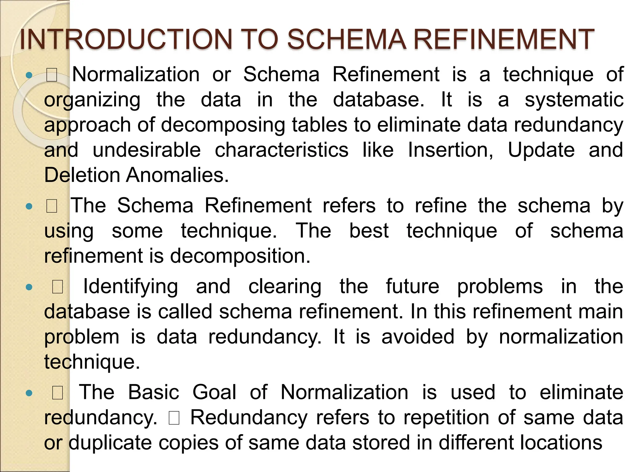
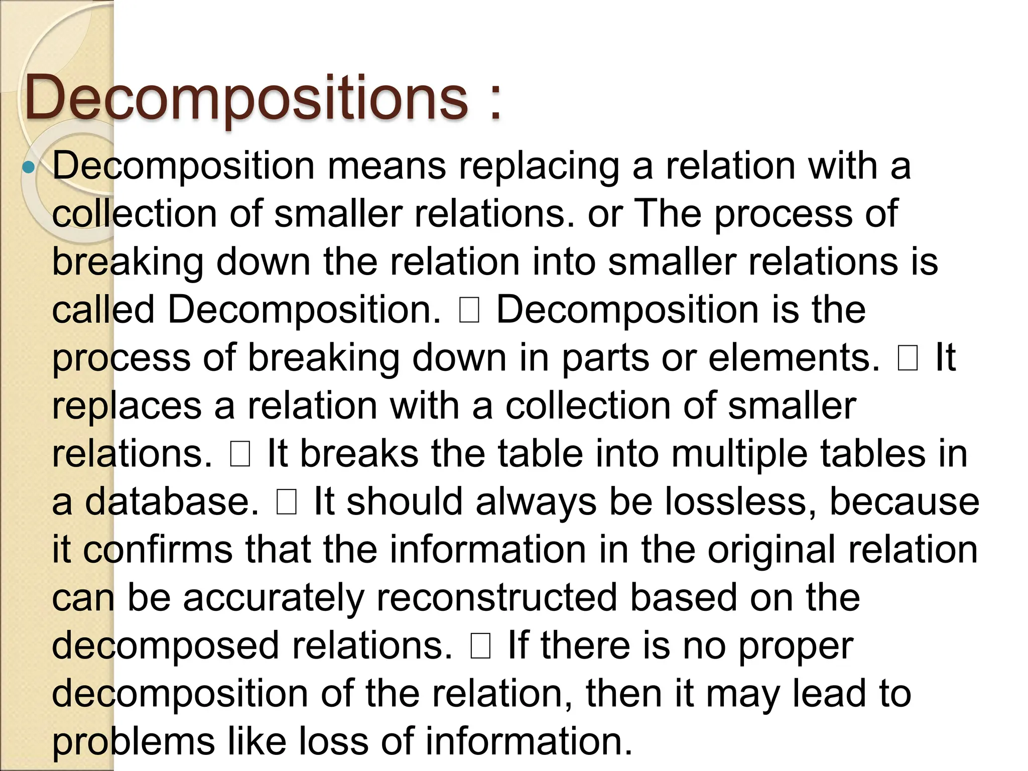
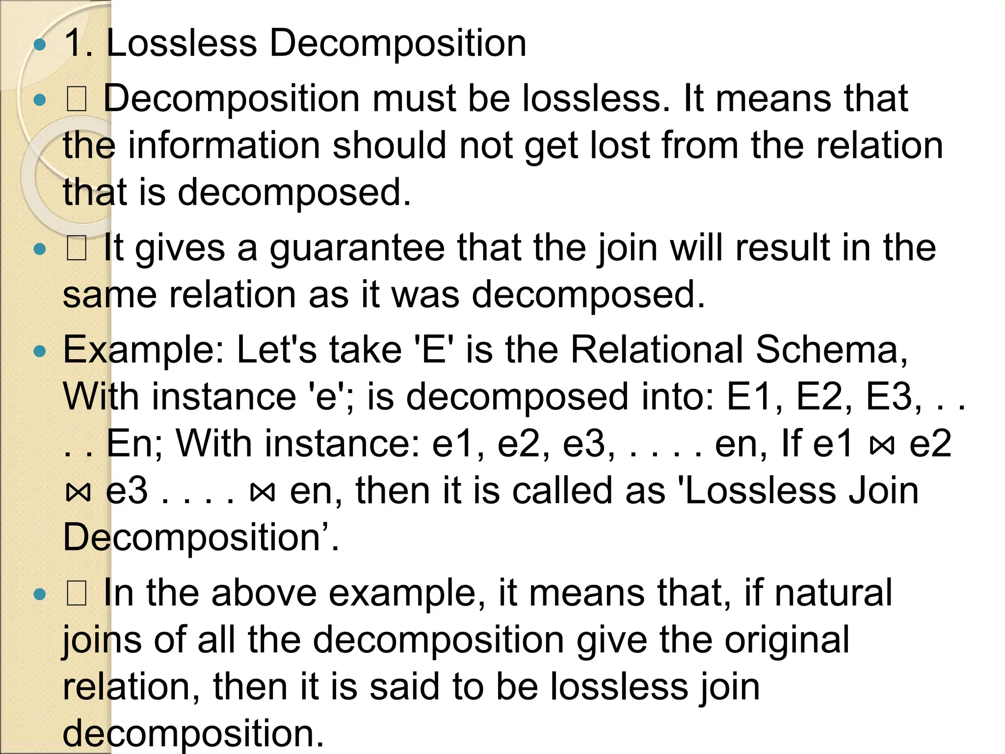
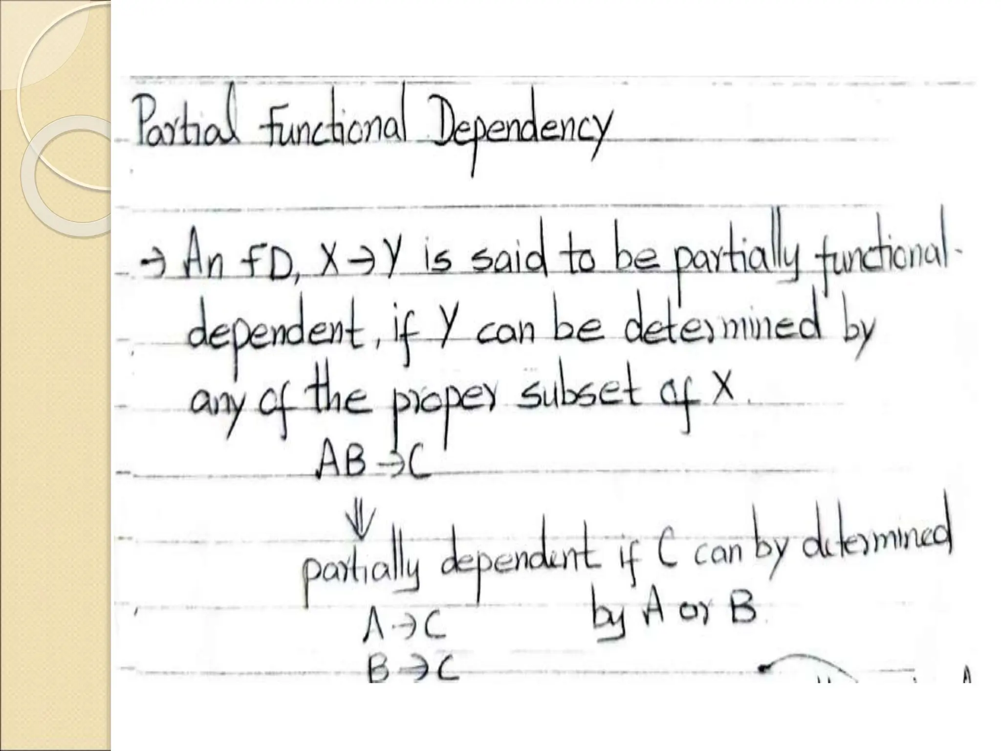
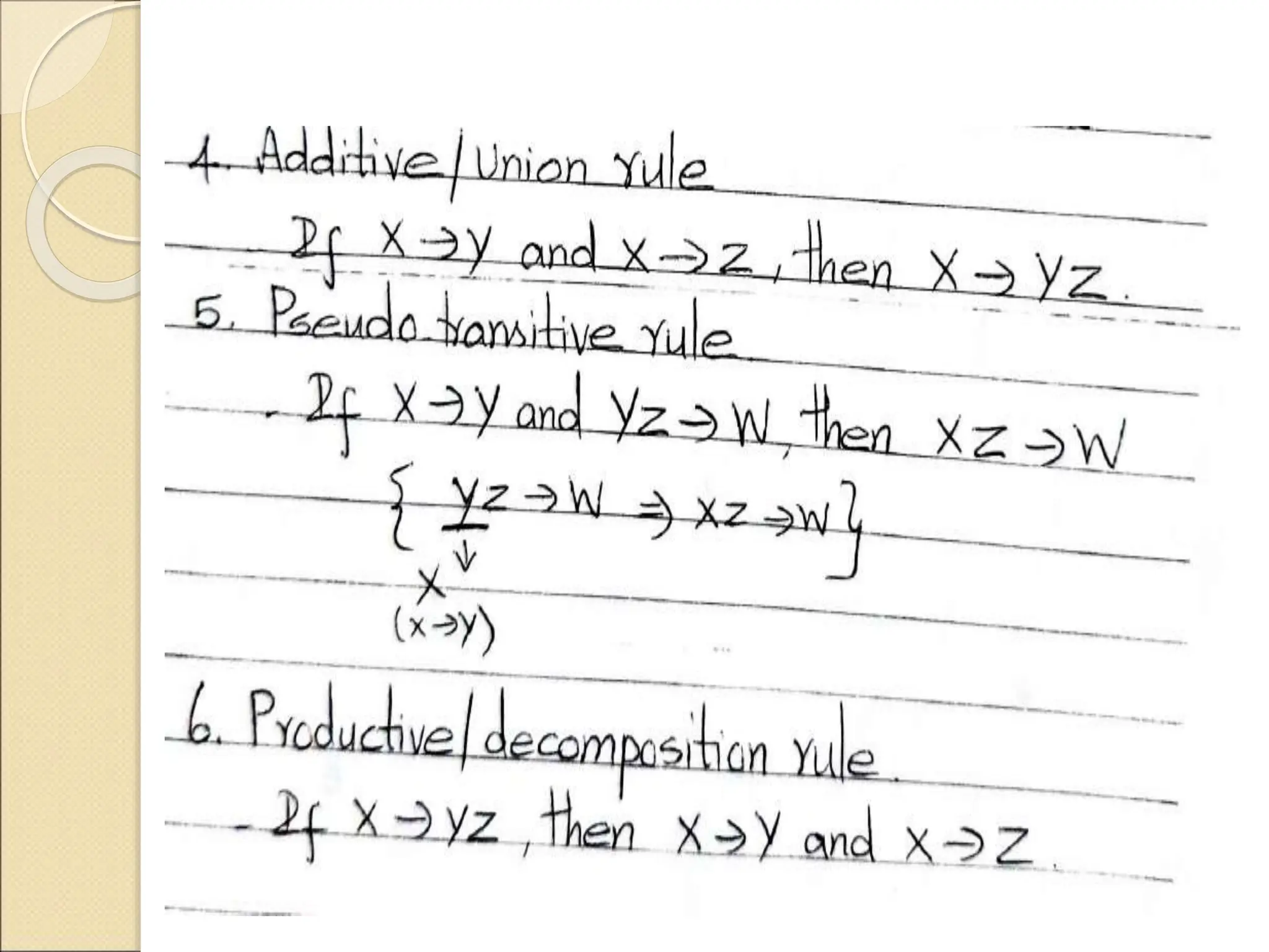
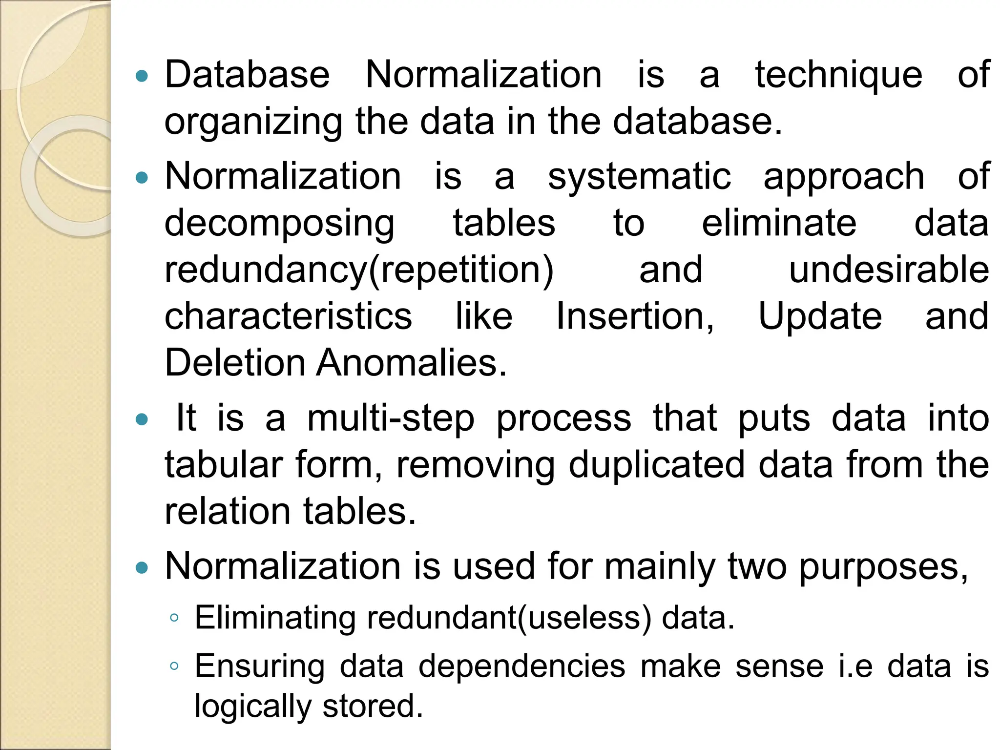
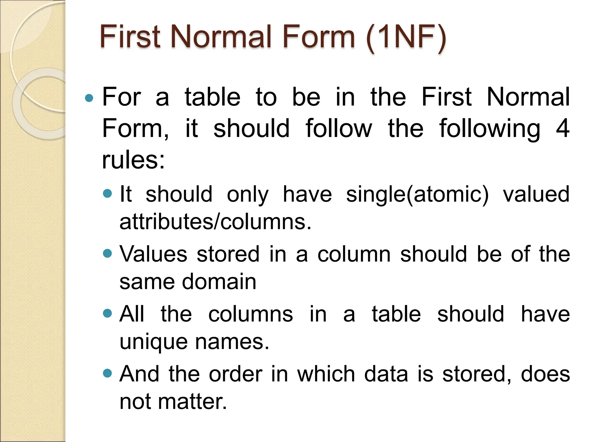
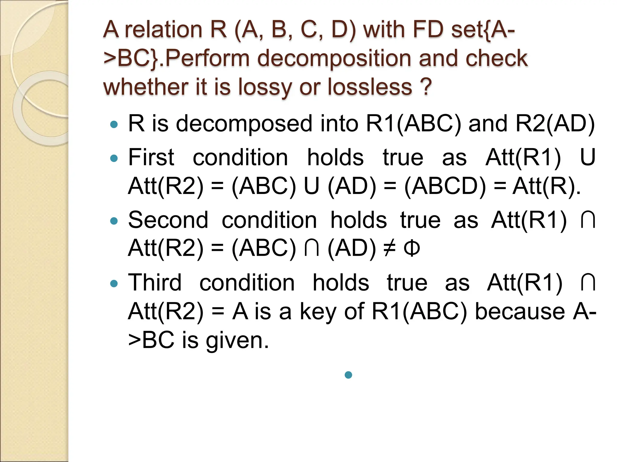
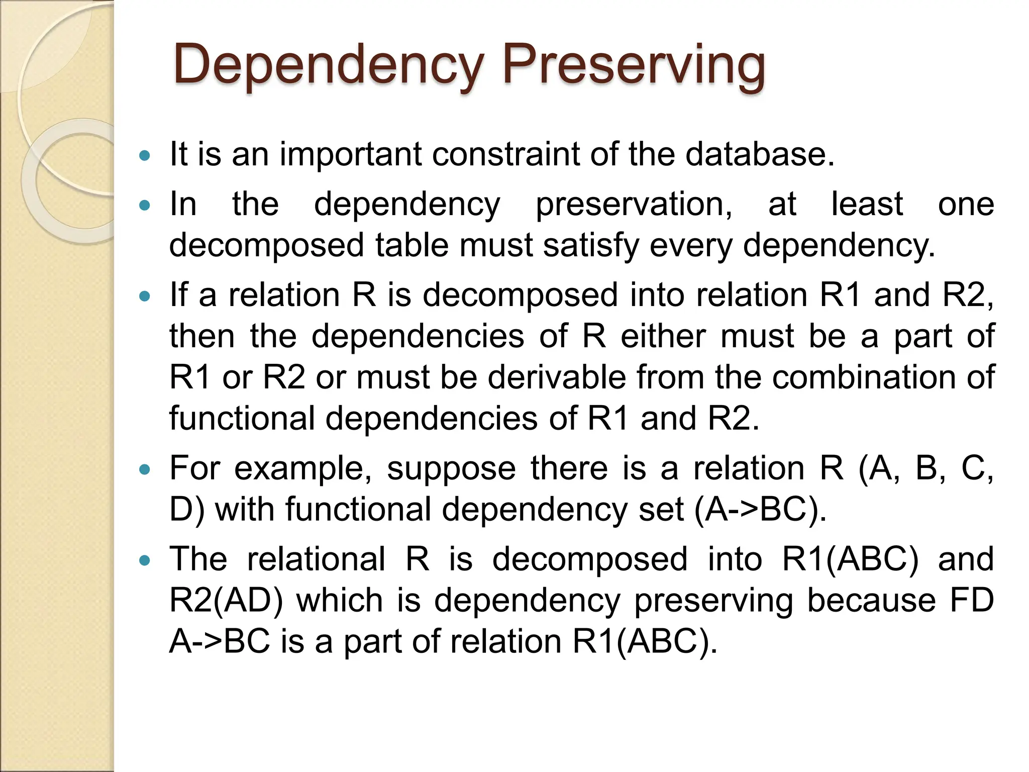
1. INTRODUCTION TO SCHEMA REFINEMENT
 Normalization or Schema Refinement is a technique of
organizing the data in the database. It is a systematic
approach of decomposing tables to eliminate data redundancy
and undesirable characteristics like Insertion, Update and
Deletion Anomalies.
 The Schema Refinement refers to refine the schema by
using some technique. The best technique of schema
refinement is decomposition.
 Identifying and clearing the future problems in the
database is called schema refinement. In this refinement main
problem is data redundancy. It is avoided by normalization
technique.
 The Basic Goal of Normalization is used to eliminate
redundancy. Redundancy refers to repetition of same data
or duplicate copies of same data stored in different locations

3. Decompositions :
 Decomposition means replacing a relation with a
collection of smaller relations. or The process of
breaking down the relation into smaller relations is
called Decomposition. Decomposition is the
process of breaking down in parts or elements. It
replaces a relation with a collection of smaller
relations. It breaks the table into multiple tables in
a database. It should always be lossless, because
it confirms that the information in the original relation
can be accurately reconstructed based on the
decomposed relations. If there is no proper
decomposition of the relation, then it may lead to
problems like loss of information.

4.  1. Lossless Decomposition
 Decomposition must be lossless. It means that
the information should not get lost from the relation
that is decomposed.
 It gives a guarantee that the join will result in the
same relation as it was decomposed.
 Example: Let's take 'E' is the Relational Schema,
With instance 'e'; is decomposed into: E1, E2, E3, . .
. . En; With instance: e1, e2, e3, . . . . en, If e1 ⋈ e2
⋈ e3 . . . . ⋈ en, then it is called as 'Lossless Join
Decomposition’.
 In the above example, it means that, if natural
joins of all the decomposition give the original
relation, then it is said to be lossless join
decomposition.

5.  2. Dependency Preservation
 Dependency is an important constraint on the
database.
 Every dependency must be satisfied by at least
one decomposed table.
 If {A → B} holds, then two sets are functional
dependent. And, it becomes more useful for
checking the dependency easily if both sets in a
same relation.
 This decomposition property can only be done by
maintaining the functional dependency.
 In this property, it allows to check the updates
without computing the natural join of the database
structure.

6.  3. Lack of Data Redundancy
 Lack of Data Redundancy is also known as a
Repetition of Information.
 The proper decomposition should not suffer from
any data redundancy.
 The careless decomposition may cause a
problem with the data.
 The lack of data redundancy property may be
achieved by Normalization process. Functional
Dependencie

7. Normalization
Different anomalies in designing a database, The idea
of normalization, Functional dependency,
Armstrong’s Axioms, Closures and their computation,
Equivalence of
Functional Dependencies (FD), Minimal Cover (proofs
not required). First Normal Form (1NF),
Second Normal Form (2NF), Third Normal Form
(3NF), Boyce Codd Normal Form (BCNF),
Lossless join and dependency preserving
decomposition, Algorithms for checking Lossless Join
(LJ) and Dependency Preserving (DP) properties.

8.  NORMAL FORMS
 Normalization is a process of evaluating and
organizing the data in database to avoid data
redundancy and inconsistency of the data.
 It is the process of decomposing the relations
with anomaly to produce smaller, well
structure relations.
 It is a formal process for describing which
attributes should be group together in a
relation based on the concept of determination

9. WHY WE NEED NORMALIZATION?
Normalization is the aim of well design
Relational Database Management System
(RDBMS). It is step by step set of rules by which
data is put in its simplest forms. We normalize
the relational database management system
because of the following reasons:
Minimize data redundancy i.e. no
unnecessarily duplication of data.
To make database structure flexible i.e. it
should be possible to add new data values and
rows without reorganizing the database
structure.

10. Different anomalies in designing
a database
 If a table is not properly normalized and
have data redundancy then it will not only
eat up extra memory space but will also
make it difficult to handle and update the
database, without facing data loss.
 Insertion, Updation and Deletion
Anomalies are very frequent if database
is not normalized.

11. Student table
rollno name branch hod office_tel
401 Akon CSE Mr. X 53337
402 Bkon CSE Mr. X 53337
403 Ckon CSE Mr. X 53337
404 Dkon CSE Mr. X 53337

12.  In the table above, we have data of 4
Computer Sci. students.
 As we can see, data for the
fields branch, hod(Head of
Department) and office_tel is repeated
for the students who are in the same
branch in the college, this is Data
Redundancy.

13. Insertion Anomaly
 Suppose for a new admission, until and
unless a student opts for a branch, data of
the student cannot be inserted, or else we
will have to set the branch information
as NULL.
 Also, if we have to insert data of 100
students of same branch, then the branch
information will be repeated for all those
100 students.
 These scenarios are nothing but Insertion
anomalies.

14. Updation Anomaly
 What if Mr. X leaves the college? or is
no longer the HOD of computer science
department?
 In that case all the student records will
have to be updated, and if by mistake
we miss any record, it will lead to data
inconsistency.
 This is Updation anomaly.

15. Deletion Anomaly
 In our Student table, two different
informations are kept together, Student
information and Branch information.
 Hence, at the end of the academic year,
if student records are deleted, we will
also lose the branch information.
 This is Deletion anomaly.

16. What is Normalization?
 Normalization is a database design
technique that reduces data redundancy
and eliminates undesirable
characteristics like Insertion, Update and
Deletion Anomalies.
 Normalization rules divides larger tables
into smaller tables and links them using
relationships.
 The purpose of Normalisation in SQL is
to eliminate redundant (repetitive) data
and ensure data is stored logically.

17. Functional dependencies in
DBMS
 A functional dependency is a constraint
that specifies the relationship between
two sets of attributes where one set can
accurately determine the value of other
sets.
 It is denoted as X → Y, where X is a set
of attributes that is capable of
determining the value of Y.
 X is called Determinant,
 Y is called the Dependent.

19. roll_no name dept_name
dept_buildin
g
42 abc CO A4
43 pqr IT A3the
44 xyz CO A4

20. valid functional dependencies:
 roll_no → { name, dept_name,
dept_building },→
◦ Here, roll_no can determine values of fields
name, dept_name and dept_building, hence a
valid Functional dependency
 roll_no → dept_name ,
◦ Since, roll_no can determine whole set of
{name, dept_name, dept_building}, it can
determine its subset dept_name also.
 dept_name → dept_building ,
◦ Dept_name can identify the dept_building
accurately, since departments with different
dept_name will also have a different
dept_building

21. invalid functional
dependencies:
 name → dept_name
◦ Students with the same name can have
different dept_name, hence this is not a
valid functional dependency.
 dept_building → dept_name
◦ There can be multiple departments in the
same building, For example, in the above
table departments ME and EC are in the
same building B2,
◦ hence dept_building → dept_name is an
invalid functional dependency.

22. Armstrong’s
axioms/properties of
functional dependencies:
 Reflexivity: If Y is a subset of X, then X→Y holds by
reflexivity rule
◦ For example, {roll_no, name} → name is valid.
 Augmentation: If X → Y is a valid dependency, then
XZ → YZ is also valid by the augmentation rule.
◦ For example, If {roll_no, name} → dept_building is valid,
hence {roll_no, name, dept_name} → {dept_building,
dept_name} is also valid.→
 Transitivity: If X → Y and Y → Z are both valid
dependencies, then X→Z is also valid by the Transitivity
rule.
◦ For example, roll_no → dept_name & dept_name →
dept_building, then roll_no → dept_building is also valid.

23. Types of Functional
dependencies in DBMS:
 Fully functional dependency
 Partial Functional Dependency
 Trivial functional dependency
 Non-Trivial functional dependency
 Multivalued functional dependency
 Transitive functional dependency

26. Trivial functional dependency
 A → B has trivial functional
dependency if B is a subset of A.
◦ {Emp_id, Emp_name} -> Emp_id is a
trivial functional dependency as Emp_id is
a subset of {Emp_id,Emp_name}.

27. Non Trivial Functional
Dependency
 when A->B holds true where B is not a
subset of A. In a relationship, if
attribute B is not a subset of attribute
A, then it is conside
◦ (Company} -> {CEO} (if we know the
Company, we knows the CEO name)
◦ But CEO is not a subset of Company, and
hence it's non-trivial functional
dependency.

28. Multivalued Dependency
 Multivalued dependency occurs in the
situation where there are multiple
independent multivalued attributes in a
single table.
 A multivalued dependency is a complete
constraint between two sets of attributes
in a relation.
 It requires that certain tuples be present
in a relation.

29.  Car(carmodel,mafyear,colour)
◦ maf_year and color are independent of
each other but dependent on car_model.
◦ In this example, these two columns are
said to be multivalue dependent on
car_model.
◦ This dependence can be represented like
this:
◦ car_model -> maf_year
◦ car_model-> colour

30. Transitive Dependency in
DBMS

31.  Company} -> {CEO} (if we know the
compay, we know its CEO's name)
 {CEO } -> {Age} If we know the CEO,
we know the Age
 Therefore according to the rule of
transitive dependency:
 { Company} -> {Age} should hold, that
makes sense because if we know the
company name, we can know his age.

34. Closure of an Attribute
 Closure of an Attribute: Closure of an
Attribute can be defined as a set of
attributes that can be functionally
determined from it.
 Closure of an attribute X is X+

35. Find the closure of A,B,C,D
given R(A,B,C,D),FD : {A->B,B-
>D,C->B}
 A+=A->B->D
◦ A+=ABD
 B+=B->D
 =BD
 C+=C->B->D
 =CBD
 D+=D

36. Closure of attribute A-
 Consider a
relation R ( A , B ,
C , D , E , F , G )
with the functional
dependencies-
 A → BC
 BC → DE
 D → F
 CF → G

 A+ = { A }
 = { A , B , C } ( Using A
→ BC )
 = { A , B , C , D , E } (
Using BC → DE )
 = { A , B , C , D , E , F }
( Using D → F )
 = { A , B , C , D , E , F ,
G } ( Using CF → G )
 Thus,
 A+ = { A , B , C , D , E ,
F , G }

37.  A → BC
 BC → DE
 D → F
 CF → G

 D+ = { D }
 = { D , F } ( Using D
→ F )

38.  A → BC
 BC → DE
 D → F
 CF → G

 { B , C }+= { B , C }
 = { B , C , D , E } ( Using
BC → DE )
 = { B , C , D , E , F } (
Using D → F )
 = { B , C , D , E , F , G } (
Using CF → G )
 Thus,
 { B , C }+ = { B , C , D , E
, F , G }


39. Given relational schema R( P Q R S T U V) having
following attribute P Q R S T U and V, also there is a
set of functional dependency denoted by FD = { P-
>Q, QR->ST, PTV->V }. Determine Closure
of (QR)+ and (PR)+
 QR+ = QR FD QR→ST
 =QRST
 PR + = PR → P → Q
 =PRQ →ST
 =PRQST

40. Given relational schema R( P Q R S T) having
following attributes P Q R S and T, also there is a set
of functional dependency denoted by FD = { P->QR,
RS->T, Q->S, T-> P }. Determine Closure of ( T )+
 T+=T → P → QR → S
 =TPQRS

41. Different kinds of keys

42. candidate key
 A candidate key may be defined as-
◦ A set of minimal attribute(s) that can
identify each tuple uniquely in the given
relation is called as a candidate key.
 OR
◦ A minimal super key is called as a
candidate key.

43.  Consider the following Student schema-
 Student ( roll , name , sex , age , address , class
, section )

 Given below are the examples of candidate keys-
 ( class , section , roll )
 ( name , address )

 These are candidate keys because each set
consists of minimal attributes required to identify
each student uniquely in the Student table.


46.  Let R = (A, B, C, D,
E, F) be a relation
scheme with the
following
dependencies-
 C → F
 E → A
 EC → D
 A → B
 Determine all
essential attributes
of the given
relation.
 Essential attributes
of the relation are-
C and E.
 So, attributes C
and E will definitely
be a part of every
candidate key.


47.  C → F
 E → A
 EC → D
 A → B
 So, we have-
 { CE }+
 = { C , E }
 = { C , E , F } ( Using C → F )
 = { A , C , E , F } ( Using E → A
)
 = { A , C , D , E , F } ( Using EC
→ D )
 = { A , B , C , D , E , F } ( Using
A → B )
 We conclude that CE can
determine all the attributes of
the given relation.
 So, CE is the only possible
candidate key of the relation.

48.  Let R = (A, B,
C, D, E) be a
relation
scheme with
the following
dependencies-
 AB → C
 C → D
 B → E
 Determine the
total number of
candidate keys

52. Closures of a set of functional
dependencies
 A Closure is a set of FDs is a set of all
possible FDs that can be derived from
a given set of FDs.
 It is also referred as a Complete set
of FDs.
 If F is used to donate the set of FDs
for relation R, then a closure of a set
of FDs implied by F is denoted by F+.

53. Find F+

56. Closure Algorithm
 Closure=X
 Repeat
 {
 For each FD u v in F
 Such that u C closure
 Then set closure = closure U v
 }
 Until there is no change to closure

58. Ssn+
a) ssn+
result=ssn
repeat
{
pno →(pname,ploc) (u v)
Pno C ssn
}

59. result=ssn
repeat
{
ssn →ename (u v)
ssn C ssn
Then result ssn U ename
Result=(ssn,ename)
}

68. Normalization Rule
 Normalization rules are divided into
the following normal forms:
 First Normal Form
 Second Normal Form
 Third Normal Form
 BCNF
 Fourth Normal Form

69.  Database Normalization is a technique of
organizing the data in the database.
 Normalization is a systematic approach of
decomposing tables to eliminate data
redundancy(repetition) and undesirable
characteristics like Insertion, Update and
Deletion Anomalies.
 It is a multi-step process that puts data into
tabular form, removing duplicated data from the
relation tables.
 Normalization is used for mainly two purposes,
◦ Eliminating redundant(useless) data.
◦ Ensuring data dependencies make sense i.e data is
logically stored.

70. First Normal Form (1NF)
 For a table to be in the First Normal
Form, it should follow the following 4
rules:
 It should only have single(atomic) valued
attributes/columns.
 Values stored in a column should be of the
same domain
 All the columns in a table should have
unique names.
 And the order in which data is stored, does
not matter.

71. roll_no name subject
101 Akon OS, CN
103 Ckon Java
102 Bkon C, C++

72.  Our table already satisfies 3 rules out
of the 4 rules, as all our column
names are unique, we have stored
data in the order we wanted to and we
have not inter-mixed different type of
data in columns.
 But out of the 3 different students in
our table, 2 have opted for more than
1 subject.
 And we have stored the subject
names in a single column. But as per
the 1st Normal form each column

73. How to solve this Problem?
roll_no name subject
101 Akon OS
101 Akon CN
103 Ckon Java
102 Bkon C
102 Bkon C++

74.  By doing so, although a few values
are getting repeated but values for
the subject column are now atomic for
each record/row.
 Using the First Normal Form, data
redundancy increases, as there will be
many columns with same data in
multiple rows but each row as a whole
will be unique.

75. Second Normal Form
 For a table to be in the Second
Normal Form, it must satisfy two
conditions:
◦ The table should be in the First Normal
Form.
◦ There should be no Partial Dependency.

76. What is Dependency?
 Let's take an example of a Student table
with
columns student_id, name, reg_no bran
ch and address .
 In this table, student_id is the primary
key and will be unique for every row,
hence we can use student_id to fetch
any row of data from this table
 Even for a case, where student names
are same, if we know the student_id we
can easily fetch the correct record.

77. student_id name reg_no branch address
10 Akon 07-WY CSE Kerala
11 Akon 08-WY IT Gujarat

78.  Hence we can say a Primary Key for
a table is the column or a group of
columns(composite key) which can
unique
 if I ask for name of student
with student_id 10 or 11, I will get it.
 So all I need is student_id and every
other column depends on it, or can be
fetched using it.
 This is Dependency and we also call
it Functional Dependency.

79. Partial Dependency
 For a simple table like Student, a single
column like student_id can uniquely
identfy all the records in a table.
 But this is not true all the time.
 Let's create another table for Subject,
which will
have subject_id and subject_name field
s and subject_id will be the primary key.

80. Subject
subject_id(Primary Key) subject_name
1 Java
2 C++
3 Php

81.  Now we have a Student table with
student information and another
table Subject for storing subject
information.
 Let's create another table Score, to
store the marks obtained by students
in the respective subjects.
 We will also be saving name of the
teacher who teaches that subject
along with marks.

82. Score
score_id student_id subject_id marks teacher
1 10 1 70 Java
Teacher
2 10 2 75 C++ Teacher
3 11 1 80 Java
Teacher

83.  In the score table we are saving the student_id to
know which student's marks are these
and subject_id to know for which subject the marks
are for.
 Together, student_id + subject_id forms a Candidate
Key for this table, which can be the Primary key
 Now if you look at the Score table, we have a column
names teacher which is only dependent on the
subject, for Java it's Java Teacher and for C++ it's C++
Teacher & so on.
 primary key for this table is a composition of two
columns which is student_id & subject_id but the
teacher's name only depends on subject, hence
the subject_id, has nothing to do with student_id.
 This is Partial Dependency, where an attribute in a

84. How to remove Partial
Dependency
 There can be many different solutions
for this, but out objective is to remove
teacher's name from Score table.
 The simplest solution is to remove
columns teacher from Score table and
add it to the Subject table. Hence, the
Subject table will become:

85. The simplest solution is to remove
columns teacher from Score table and add it
to the Subject table. Hence, the Subject table
will become:
id subject_name teacher
1 Java Java Teacher
2 C++ C++ Teacher
3 Php Php Teacher

86. And our Score table is now in the second
normal form, with no partial dependency
score_id student_id subject_id marks
1 10 1 70
2 10 2 75
3 11 1 80

87. Third Normal Form (3NF)
 A relation will be in 3NF
◦ if it is in 2NF and not contain any
transitive partial dependency.
 3NF is used to reduce the data
duplication.
 It is also used to achieve the data
integrity.
 If there is no transitive dependency for
non-prime attributes, then the relation
must be in third normal form.

88. Employee Table
EMP_ID EMP_NAM
E
EMP_ZIP EMP_STAT
E
EMP_CITY
222 Harry 201010 UP Noida
333 Stephan 02228 US Boston
444 Lan 60007 US Chicago

89.  Super key in the table above:
◦ {EMP_ID}, {EMP_ID, EMP_NAME}, {EMP_ID, E
M
 Non-prime attributes: In the given table,
all attributes except EMP_ID are non-prime.
◦ Here, EMP_STATE & EMP_CITY dependent on
EMP_ZIP and
◦ EMP_ZIP dependent on EMP_ID.
◦ The non-prime attributes (EMP_STATE,
EMP_CITY) transitively dependent on super
key(EMP_ID). It violates the rule of third normal
form.(ab,bc ac)
◦ So need to move the EMP_CITY and
EMP_STATE to the new <EMPLOYEE_ZIP>
table, with EMP_ZIP as a Primary key.

90. Employee Table
EMP_ID EMP_NAME EMP_ZIP
222 Harry 201010
333 Stephan 02228
444 Lan 60007

91. EMPLOYEE_ZIP table
EMP_ZIP EMP_STATE EMP_CITY
201010 UP Noida
02228 US Boston
60007 US Chicago

92. Boyce Codd normal form (BCNF)
 BCNF is the advance version of 3NF.
It is stricter than 3NF.
◦ A table is in BCNF if every functional
dependency X → Y, X is the super key of
the table.
◦ For BCNF, the table should be in 3NF, and
for every FD, LHS is super key.

93. EMPLOYEE table
EMP_ID EMP_COU
NTRY
EMP_DEPT DEPT_TYP
E
EMP_DEPT
_NO
264 India Designing D394 283
264 India Testing D394 300
364 UK Stores D283 232

94.  In the above table Functional
dependencies are as follows:
◦ EMP_ID → EMP_COUNTRY
◦ EMP_DEPT → {DEPT_TYPE, EMP_DE
PT_NO}
 Candidate key: {EMP-ID, EMP-
DEPT}
 The table is not in BCNF because
neither EMP_DEPT nor EMP_ID
alone are keys.
 To convert the given table into BCNF,
we decompose it into three tables:

95. EMP_COUNTRY table:
EMP_ID EMP_COUNTRY
264 India
264 India

96. EMP_DEPT table:
EMP_DEPT DEPT_TYPE EMP_DEPT_NO
Designing D394 283
Testing D394 300
Stores D283 232
Developing D283 549

97. EMP_DEPT_MAPPING table
EMP_ID EMP_DEPT
D394 283
D394 300
D283 232
D283 549

98.  Candidate keys:
◦ For the first table: EMP_ID
For the second table: EMP_DEPT
For the third table: {EMP_ID,
EMP_DEPT}
 Functional dependencies:
◦ EMP_ID → EMP_COUNTRY
◦ EMP_DEPT → {DEPT_TYPE, EMP_D
EPT_NO}
 Now, this is in BCNF because left side
part of both the functional
dependencies is a key.

99. Fourth Normal Form (4NF)
 For a table to satisfy the Fourth
Normal Form, it should satisfy the
following two conditions:
◦ It should be in the Boyce-Codd Normal
Form.
◦ And, the table should not have any Multi-
valued Dependency.

100. STUDENT
STU_ID COURSE HOBBY
21 Computer Dancing
21 Math Singing
34 Chemistry Dancing

101.  The given STUDENT table is in 3NF, but the
COURSE and HOBBY are two independent
entity. Hence, there is no relationship
between COURSE and HOBBY.
 In the STUDENT relation, a student with
STU_ID, 21 contains two
courses, Computer and Math and two
hobbies, Dancing and Singing. So there is a
Multi-valued dependency on STU_ID, which
leads to unnecessary repetition of data.
 So to make the above table into 4NF, we can
decompose it into two tables:

102. STUDENT_COURSE
STU_ID COURSE
21 Computer
21 Math
34 Chemistry

103. STUDENT_HOBBY
STU_ID HOBBY
21 Dancing
21 Singing
34 Dancing

104. Relational Decomposition
 When a relation in the relational model is not in
appropriate normal form then the
decomposition of a relation is required.
 In a database, it breaks the table into multiple
tables.
 If the relation has no proper decomposition,
then it may lead to problems like loss of
information.
 Decomposition is used to eliminate some of
the problems of bad design like anomalies,
inconsistencies, and redundancy.

105. Types of Decomposition

106. Lossless Decomposition
 If the information is not lost from the
relation that is decomposed, then the
decomposition will be lossless.
 The lossless decomposition guarantees
that the join of relations will result in the
same relation as it was decomposed.
 The relation is said to be lossless
decomposition if natural joins of all the
decomposition give the original relation.

107.  Lossless Join Decomposition
 If we decompose a relation R into
relations R1 and R2,
 Decomposition is lossy if R1 ⋈ R2 ⊃
R
 Decomposition is lossless if R1 ⋈ R2
= R

108. EMPLOYEE_DEPARTMENT
table:
EMP_ID EMP_NA
ME
EMP_AG
E
EMP_CI
TY
DEPT_ID DEPT_N
AME
22 Denim 28 Mumbai 827 Sales
33 Alina 25 Delhi 438 Marketing
46 Stephan 30 Bangalor
e
869 Finance
52 Katherine 36 Mumbai 575 Productio
n
60 Jack 40 Noida 678 Testing

109. The above relation is
decomposed into two relations
EMPLOYEE and DEPARTMENT
EMP_ID EMP_NAME EMP_AGE EMP_CITY
22 Denim 28 Mumbai
33 Alina 25 Delhi
46 Stephan 30 Bangalore
52 Katherine 36 Mumbai
60 Jack 40 Noida

110. DEPARTMENT table
DEPT_ID EMP_ID DEPT_NAME
827 22 Sales
438 33 Marketing
869 46 Finance
575 52 Production
678 60 Testing

111. Employee ⋈ Department
EMP_ID EMP_NA
ME
EMP_AG
E
EMP_CI
TY
DEPT_ID DEPT_N
AME
22 Denim 28 Mumbai 827 Sales
33 Alina 25 Delhi 438 Marketing
46 Stephan 30 Bangalor
e
869 Finance
52 Katherine 36 Mumbai 575 Productio
n
60 Jack 40 Noida 678 Testing

112. To check for lossless join decomposition
using FD set, following conditions must
hold:
 Union of Attributes of R1 and R2 must be
equal to attribute of R. Each attribute of R
must be either in R1 or in R2.
◦ Att(R1) U Att(R2) = Att(R)
 Intersection of Attributes of R1 and R2 must
not be NULL.
◦ Att(R1) ∩ Att(R2) ≠ Φ
 Common attribute must be a key for at least
one relation (R1 or R2)
◦ Att(R1) ∩ Att(R2) -> Att(R1) or Att(R1) ∩ Att(R2) ->
Att(R2)

113. A relation R (A, B, C, D) with FD set{A-
>BC}.Perform decomposition and check
whether it is lossy or lossless ?
 R is decomposed into R1(ABC) and R2(AD)
 First condition holds true as Att(R1) U
Att(R2) = (ABC) U (AD) = (ABCD) = Att(R).
 Second condition holds true as Att(R1) ∩
Att(R2) = (ABC) ∩ (AD) ≠ Φ
 Third condition holds true as Att(R1) ∩
Att(R2) = A is a key of R1(ABC) because A-
>BC is given.


114. Dependency Preserving
 It is an important constraint of the database.
 In the dependency preservation, at least one
decomposed table must satisfy every dependency.
 If a relation R is decomposed into relation R1 and R2,
then the dependencies of R either must be a part of
R1 or R2 or must be derivable from the combination of
functional dependencies of R1 and R2.
 For example, suppose there is a relation R (A, B, C,
D) with functional dependency set (A->BC).
 The relational R is decomposed into R1(ABC) and
R2(AD) which is dependency preserving because FD
A->BC is a part of relation R1(ABC).